Computing partition functions in the one clean qubit model

Abstract

We present a method to approximate partition functions of quantum systems using mixed-state quantum computation. For positive semi-definite Hamiltonians, our method has expected running-time that is almost linear in $(M/(\epsilon_{\rm rel}\mathcal{Z}))^{2}$, where $M$ is the dimension of the quantum system, $\mathcal{Z}$ is the partition function, and $\epsilon_{\rm rel}$ is the relative precision. It is based on approximations of the exponential operator as linear combinations of certain operators related to block-encoding of Hamiltonians or Hamiltonian evolutions. The trace of each operator is estimated using a standard algorithm in the one clean qubit model. For large values of $\mathcal{Z}$, our method may run faster than exact classical methods, whose complexities are polynomial in $M$. We also prove that a version of the partition function estimation problem within additive error is complete for the so-called DQC1 complexity class, suggesting that our method provides a super-polynomial speedup for certain parameter values. To attain a desired relative precision, we develop a classical procedure based on a sequence of approximations within predetermined additive errors that may be of independent interest.

I Introduction

One of the most important quantities used to describe a physical system in thermodynamic equilibrium is the partition function $\mathcal{Z}$. Many thermodynamic properties, such as the free energy or entropy, can then be derived from $\mathcal{Z}$ using simple mathematical relations Pat72 . Partition functions also appear naturally in many other problems in mathematics and computer science, such as counting the solutions of constraint satisfaction problems BG05 . Therefore, developing novel algorithms for partition functions is of great importance Bra08 ; PW09 ; NDR+09 ; CS16 ; HMS19 .

In this paper, we present a method for approximating partition functions using the one clean qubit model of computation. In this model, one qubit is initialized in a pure state, in addition to $n$ qubits in the maximally mixed state KL98 . This is in contrast to standard quantum computation, where the many-qubit initial state is pure NC01 . The one clean qubit model has attracted significant attention as it appears that some problems can be solved efficiently within this model for which no efficient classical algorithms are known to exist PBL+04 ; SJ08 ; CM18 . Additionally, this model is practically relevant for mixed-state quantum computation, e.g., it is suitable to describe liquid-state NMR LKC+02 ; NSO+05 , and for quantum metrology BS08 . We demonstrate further advantages of the one clean qubit model by describing a method to estimate partition functions of quantum systems.

Our main result is a method that outputs an estimate $\hat{\mathcal{Z}}$ of $\mathcal{Z}$ within given relative precision $\epsilon_{\rm rel}>0$ and with high success probability $(1-\delta)<1$. To achieve this goal we first give algorithms in the one clean qubit model that can estimate partition functions of certain $m$-qubit systems within a desired additive error. The basic idea behind these algorithms is the fact that $\mathcal{Z}$ can be approximated from linear combinations of the traces of certain unitary operators. We present two approaches: one in which the unitaries are constructed from a block-encoding of the Hamiltonian and another in which they are constructed from Hamiltonian evolutions. The trace of each such unitary can be estimated by repeated uses of the well-known trace-estimation algorithm of Fig. 1, which allows us to compute $\mathcal{Z}$ with additive error. Finally, we obtain an estimate of $\mathcal{Z}$ within a desired relative error by iterating multiple additive-error estimations.

For positive semi-definite Hamiltonians, our algorithm for obtaining relative-error estimates of the partition function has expected running-time that is almost linear in $(M/(\epsilon_{\rm rel}\mathcal{Z}))^{2}$, where $M=2^{m}$. In contrast, the runtime of a classical method based on exact diagonalization scales as $M^{3}$ and the runtime of the kernel polynomial method scales as $M$ weisse2006kernel . Our method can thus provide a significant (super-polynomial) speedup in cases where $\mathcal{Z}$, or the temperature, is sufficiently large. However, the improvement is less pronounced or may be lost when $\mathcal{Z}$ is small, which corresponds to the low-temperature regime. In this regime, estimating the partition function is known to be computationally difficult Sly10 ; HMS19 . Further, numerous complexity theoretic results effectively rule out the possibility of having efficient general-purpose algorithms for estimating the partition function. Exactly computing partition functions of classical systems, e.g., the Ising model is #P-hard JS93 , and even approximating them to a multiplicative error can be NP-hard; see Ref. MQ13 for some results. While efficient polynomial-time approximation algorithms exist for high-temperature partition functions, these algorithms have not been shown to work at low temperatures, i.e., temperatures below the critical point HMS19 . Our method as well as known quantum algorithms such as Ref. PW09 can work at any temperature, even though the complexities may not always be favorable.

The complexity of additive-error estimates of the partition function has also received attention, notably in the context of quantum computation. It is known that for certain lattice models this problem can be either BQP-complete or DQC1-complete, but only in complex parameter regimes (complex temperatures) that do not correspond to physical scenarios DDVM11 . In a physically relevant setting (real temperature), Brandão showed that it is DQC1-hard to estimate the normalized partition function of certain $\log m$-local Hamiltonians within $1/\mathrm{poly}(m)$ additive error at temperature that is $\Omega(1/\mathrm{poly}(m))$ Bra08 . Our results imply that this problem is in fact DQC1-complete. This suggests that in some cases our algorithm provides a super-polynomial speed-up.

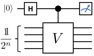
Figure 1: The trace-estimation algorithm to compute the renormalized trace of a unitary operator $V$. The clean (ancilla) qubit is initialized in the state $\ket{0}$ and then acted on with the Hadamard gate ${\rm H}$. The remaining $n$ qubits are initialized in the completely mixed state ${\mathchoice{\rm 1\mskip-4.0mul}{\rm 1\mskip-4.0mul}{\rm 1\mskip-4.5mul}{\rm 1\mskip-5.0mul}}/2^{n}$. The filled circle denotes that $V$ is applied conditional on the state of the ancilla being $\ket{1}$. Repeated projective measurements of the ancilla-qubit Pauli operator $\sigma_{x}$, resulting in $\pm 1$ outcomes, provide an estimate of the expectation $\langle\sigma_{x}\rangle=\mathrm{Re}\mathrm{Tr}[V]/2^{n}$.

The rest of the paper is organized as follows. In Sec. II we state our assumptions and introduce the partition function problem where the goal is to estimate $\mathcal{Z}$ within given relative error. In Sec. III we describe the one clean qubit model and introduce the DQC1 complexity class. In Sec. IV we provide two approximations to the exponential operator as specific linear combinations of unitaries, which will be used by our method. The unitaries in the approximation are related to block-encoding of Hamiltonians or Hamiltonian simulation, and we describe the implementations of these in Sec. V. In Sec. VI we provide our main algorithms. In Sec. VII we demonstrate the correctness of our method and in Sec. VIII we establish its complexity. In Sec. IX we show that a version of the partition function problem is DQC1-complete and we conclude in Sec. X.

We give some technical proofs in Appendices A, B, and C. In Appendix D we develop a classical procedure to estimate quantities with a given relative error and success probability, from estimations with suitable additive errors and success probabilities. This procedure is formulated under fairly general assumptions and it can be applied to a wide range of problems beyond the one considered in this paper. Finally, in Appendix E we bound the complexity of our algorithms for obtaining relative estimates to the partition function.

II Problem statement

We consider a discrete, $M$-dimensional quantum system with Hamiltonian $H$. In the canonical ensemble, the partition function is

$$\mathcal{Z}:=\text{Tr}\left(e^{-\beta H}\right)\;,$$ (1)

where $\beta\geq 0$ is the inverse temperature. That is, $\beta=1/k_{\rm B}T$, with $k_{\rm B}$ the Boltzmann constant and $T$ the temperature. For simplicity, we will focus on systems composed of $m$ qubits, where $m=\log_{2}(M)$. Nevertheless, if one is interested in partition functions of quantum systems obeying different particle statistics, such as bosonic or fermionic systems, the results in Refs. SOGKL02 ; SOKG03 may be used to represent the corresponding operators in terms of Pauli operators acting on qubits. The techniques developed here can then be used to study such systems. Formally, we define the partition function problem (PFP) as follows:

Definition 1 (PFP).

Given a Hamiltonian $H$, an inverse temperature $\beta\geq 0$, a relative precision parameter $\epsilon_{\rm rel}>0$, and a probability of error $\delta>0$, the goal is to output a positive number $\hat{\mathcal{Z}}$ such that

$$\left|\hat{\mathcal{Z}}-{\mathcal{Z}}\right|\leq\epsilon_{\rm rel}{\mathcal{Z}}\;,$$ (2)

with probability at least $(1-\delta)$.

The reason why we focus on relative approximations of the partition function is because they translate to additive approximations for the estimation of extensive thermodynamic quantities such as entropy and free energy. For example, the free energy in thermodynamic equilibrium is given by $F=-(1/\beta)\log Z$. Using the estimate $\hat{\mathcal{Z}}$ to obtain an estimate $\hat{F}$, we obtain $|F-\hat{F}|=O(\epsilon_{\rm rel}/\beta)$. We will also consider additive approximations of $\mathcal{Z}$ in our discussion — this is in fact the partition function problem studied in Ref. Bra08 , for which a quantum algorithm in the circuit model is given. We show in Sec. VI that the two problems are related.

Our main goal is to provide an algorithm that uses the one clean qubit model to solve the PFP. We will focus on Hamiltonians that have the form $H=\sum_{l=1}^{L}\alpha_{l}H_{l}$, $\alpha_{l}>0$, $L=O(\text{poly}(m))$, and where each $H_{l}$ is either a unitary operator or a projector. We require that there exist efficient quantum circuits to implement either each $H_{l}$ (when it is unitary) or a unitary related to each $H_{l}$ (when it is a projector), as explained in Sec. V. Defining $\alpha=\sum_{l=1}^{L}\alpha_{l}$, we work with the renormalized Hamiltonian $H\leftarrow H/\alpha$ and rescaled inverse temperature $\beta\leftarrow\beta\alpha$ in order to simplify notation. The complexities of our algorithms depend implicitly on $\alpha$ through their dependence on the inverse temperature $\beta$.

III The one clean qubit model

In the one clean qubit model, the initial state (density matrix) of a system of $n+1$ qubits is

$$\rho_{i}=\outerproduct{0}{0}\otimes\frac{{\mathchoice{\rm 1\mskip-4.0mul}{\rm 1\mskip-4.0mul}{\rm 1\mskip-4.5mul}{\rm 1\mskip-5.0mul}}}{2^{n}}\;,$$ (3)

where ${\mathchoice{\rm 1\mskip-4.0mul}{\rm 1\mskip-4.0mul}{\rm 1\mskip-4.5mul}{\rm 1\mskip-5.0mul}}$ is the identity operator over $n$ qubits. We write $\mathcal{H}_{n}\equiv\mathbb{C}^{2^{n}}$ for the Hilbert space associated with $n$-qubit quantum states. A quantum circuit $U=U_{T-1}\ldots U_{0}$ is then applied to $\rho_{i}$, where each $U_{j}$ is a two-qubit quantum gate, and a projective measurement is performed on the ancilla at the end. The outcome probabilities are $p_{0}$ and $p_{1}=1-p_{0}$, where

$$p_{0}=\mathrm{Tr}[(U\rho_{i}U^{\dagger})(\outerproduct{0}{0}\otimes{\mathchoice{\rm 1\mskip-4.0mul}{\rm 1\mskip-4.0mul}{\rm 1\mskip-4.5mul}{\rm 1\mskip-5.0mul}})]\;.$$ (4)

The complexity class DQC1 consists of decision problems that can be solved within the one clean qubit model in polynomial time (in the problem size $s$) with correctness probability $\geq 2/3$. We are allowed to act on $\rho_{i}$ with quantum circuits of length $\text{poly}(s)$, measure the ancilla, and repeat this $\mathrm{poly}(s)$ many times. In our definition, DQC1 contains the class BPP, that is, the class of problems that can be solved in time $\text{poly}(s)$ using a classical computer (probabilistic Turing machine).

Remarkably, it can be shown that the problem of estimating $\mathrm{Re}\mathrm{Tr}[V]/2^{n}$ within additive error $\Omega(1/\text{poly}(n))$, where $V$ is a quantum circuit of length $O(\text{poly}(n))$ acting on $\mathcal{H}_{n}$, is complete for the DQC1 class KL98 . That is, any other problem in DQC1 can be reduced to trace estimation. While this is not a decision problem, it can be transformed to one by simple manipulations Shep06 . In this paper, however, we will mainly focus on problems that can be reduced to trace estimation but where the number of operations or steps are sometimes exponentially large in $n$; that is, problems that are not necessarily in DQC1.

The trace-estimation algorithm is shown in Fig. 1. For a given quantum circuit $V$, the quantum state before measurement is

$$\rho_{f}=\frac{1}{2^{n+1}} (\outerproduct{0}{0}\otimes{\mathchoice{\rm 1\mskip-4.0mul}{\rm 1\mskip-4.0mul}{\rm 1\mskip-4.5mul}{\rm 1\mskip-5.0mul}}+\outerproduct{0}{1}\otimes V^{\dagger}+$$

$$+\outerproduct{1}{0}\otimes V+\outerproduct{1}{1}\otimes{\mathchoice{\rm 1\mskip-4.0mul}{\rm 1\mskip-4.0mul}{\rm 1\mskip-4.5mul}{\rm 1\mskip-5.0mul}})\;.$$ (5)

Projective measurements on $\rho_{f}$ of the ancilla Pauli operator $\sigma_{x}$ result in $\pm 1$ outcomes whose average is an estimator of $\mathrm{Re}\mathrm{Tr}[V]/2^{n}$. In particular,

$$\langle\sigma_{x}\rangle :=\mathrm{Tr}[\rho_{f}\,\sigma_{x}]$$ (6)

$$=\frac{\mathrm{Re}\mathrm{Tr}[V]}{2^{n}}\;.$$ (7)

We will then estimate the expectation $\langle\sigma_{x}\rangle$, and thus $\mathrm{Re}\mathrm{Tr}[V]$, from finitely many uses of the trace-estimation algorithm. We obtain:

Lemma 1.

Given $\varepsilon>0$, $\delta_{0}>0$, and a quantum circuit $V$ acting on $n$ qubits, we can obtain an estimate $\hat{\xi}_{V}\in\mathbb{R}$ that satisfies

$$\left|\hat{\xi}_{V}-\mathrm{Re}\mathrm{Tr}[V]\right|\leq\varepsilon\;,$$ (8)

with probability at least $(1-\delta_{0})$, using the trace-estimation algorithm $Q=\lceil(2^{2n+1}/\varepsilon^{2})\log(2/\delta_{0})\rceil$ times.

The proof of Lemma 1 is a simple consequence of Hoeffding’s inequality Hoe63 and is given in Appendix A. If $s_{x}$ is the average of the measurement outcomes of $\sigma_{x}$, the estimate is simply $\hat{\xi}_{V}=2^{n}s_{x}$.

For our method, we will be interested in estimating the trace of a given block of a unitary matrix within given additive error. More specifically, let $W$ be a quantum circuit defined on a system of $m+m^{\prime}$ qubits. We obtain:

Corollary 1.

Given $\varepsilon>0$, $\delta_{0}>0$, and a quantum circuit $W$ acting on $m+m^{\prime}$ qubits, we can obtain an estimate $\hat{\chi}_{W}\in\mathbb{R}$ that satisfies

$$\left|\hat{\chi}_{W}-\mathrm{Re}\mathrm{Tr}[\bra{0}_{m^{\prime}}W\ket{0}_{m^{\prime}}]\right|\leq\varepsilon\;,$$ (9)

with probability at least $(1-\delta_{0})$, using the trace-estimation algorithm $Q=\lceil(2^{2(m+m^{\prime})+1}/\varepsilon^{2})\log(2/\delta_{0})\rceil$ times. Here, $\ket{0}_{m^{\prime}}\in\mathcal{H}_{m^{\prime}}$ is the zero state of $m^{\prime}$ qubits and $\bra{0}_{m^{\prime}}W\ket{0}_{m^{\prime}}$ is the corresponding block of $W$.

Corollary 1 follows from the observation that there is a quantum circuit $V$, acting on $n=m+2m^{\prime}$ qubits, and

$$\frac{1}{2^{m^{\prime}}}\mathrm{Tr}[V]=\mathrm{Tr}[\bra{0}_{m^{\prime}}W\ket{0}_{m^{\prime}}]\;;$$ (10)

see Ref. SJ08 . The unitary $V$ is described in Fig 2. The proof of Cor. 1 follows from Lemma 1, where the number of qubits is $n=m+2m^{\prime}$. The estimate in this case is $\hat{\chi}_{W}=2^{m+m^{\prime}}s_{x}$.

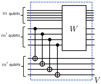
Figure 2: Quantum circuit $V$ that satisfies $\frac{1}{2^{m^{\prime}}}\mathrm{Tr}[V]=\mathrm{Tr}[\bra{0}_{m^{\prime}}W\ket{0}_{m^{\prime}}]$. The first operations are a sequence of $m^{\prime}$ CNOT gates on the corresponding pairs of ancilla qubits SJ08 .

IV Approximations of the exponential operator

Our method for estimating the partition function in the one clean qubit model proceeds by approximating it as a weighted sum of traces of unitary operators. Each such trace can then be computed through repeated uses of the trace-estimation algorithm of Fig. 1. We now describe two approximations of the exponential operator that will be used.

IV.1 Chebyshev approximation

The first approximation is based on Chebyshev polynomials. If the $m$-qubit Hamiltonian satisfies $\|H\|\leq 1$, we obtain

$$e^{-\beta H}=\sum_{k=-\infty}^{\infty}(-1)^{k}I_{k}(\beta)T_{k}(H)\;.$$ (11)

Here, $I_{k}(x)\in\mathbb{R}$ are the modified Bessel functions of the first kind. $T_{k}(H)$ is an operator acting on $\mathcal{H}_{m}$ obtained by replacing $x$ by $H$ in $T_{k}(x)$, the $k$-th Chebyshev polynomial of the first kind — see Appendix B. We will approximate the exponential operator by a finite sum, by noticing that $I_{k}(\beta)$ decays exponentially fast in the large $k$ limit (for fixed $\beta$). In Appendix B we show:

Lemma 2.

Given $\epsilon_{\rm abs}>0$ and $\beta\geq 0$, we can choose $K=\lceil m+e\beta+\log_{2}(1/\epsilon_{\rm abs})+2\rceil$ such that

$$\|S_{K}-e^{-\beta H}\|_{1}\leq\epsilon_{\rm abs}/2\;,$$ (12)

where $\|\cdot\|_{1}$ denotes the trace norm and

$$S_{K} :=\sum_{k=-K}^{K}(-1)^{k}I_{k}(\beta)T_{k}(H)\;.$$ (13)

Equivalently, $S_{K}=I_{0}(\beta)+2\sum_{k=1}^{K}(-1)^{k}I_{k}(\beta)T_{k}(H)$. To represent $S_{K}$ as a linear combination of suitable operations for our method, we further assume that there exist unitary operators $W_{H}$ and $\tilde{G}$, acting on $m+m^{\prime}$ qubits, that satisfy

$$T_{k}(H)=\langle 0|_{m^{\prime}}\tilde{G}^{\dagger}(W_{H})^{k}\tilde{G}|0\rangle_{m^{\prime}}\,.$$ (14)

The operation $W_{H}$ in Eq. (14) is the “unitary iterate” or the quantum walk operator as used recently for Hamiltonian simulation LC19 or linear algebra problems CKS17 , and $\tilde{G}$ is a related state-preparation unitary. We describe $W_{H}$ and $\tilde{G}$ in detail in Sec. V.1.

Our first approach solves the PFP using the relation

$$\mathrm{Tr}[S_{K}]=I_{0}(\beta) M+2\sum_{k=1}^{K}(-1)^{k}I_{k}(\beta)$$

$$\times\mathrm{Re}\mathrm{Tr}[\bra{0}_{m^{\prime}}\tilde{G}^{\dagger}(W_{H})^{k}\tilde{G}\ket{0}_{m^{\prime}}]\;,$$ (15)

which is an $\epsilon_{\rm abs}/2$ approximation to $\mathcal{Z}$. We can use the construction in Fig. 2 in the trace-estimation algorithm of Fig. 1 to obtain $\mathrm{Re}\mathrm{Tr}[\bra{0}_{m^{\prime}}\tilde{G}^{\dagger}(W_{H})^{k}\tilde{G}\ket{0}_{m^{\prime}}]$.

IV.2 LCU approximation

The second approximation is based on the so-called Hubbard-Stratonovich transformation Hub59 ; CS16 . If $H\geq 0$, we obtain

$$e^{-\beta H}=\frac{1}{\sqrt{2\pi}}\int dy\;e^{-y^{2}/2}e^{-iy\sqrt{2\beta H}}\;.$$ (16)

Here, $\sqrt{H}$ is also a Hermitian operator that refers to one of the square roots of $H$. As the eigenvalues of $H$ are non-negative, this case appears to be more restrictive. Nevertheless, the assumption $H\geq 0$ may be met after a simple pre-processing step that shifts $H$ — see Sec. V.

We wish to obtain an approximation of $e^{-\beta H}$ by a finite linear combination of unitaries following Eq. (16). This approximation is analyzed in Appendix C and was also studied in Ref. CS16 . If $\|H\|\leq 1$, we obtain:

Lemma 3.

Given $\epsilon_{\rm abs}>0$ and $\beta\geq 0$, we can choose

$$J =\lceil 12(\sqrt{\beta}+\sqrt{m+\log_{2}(1/\epsilon_{\rm abs})})\sqrt{m+\log_{2}(1/\epsilon_{\rm abs})}\rceil$$ (17)

and

$$\delta y=\left(2(\sqrt{\beta}+\sqrt{m+\log_{2}(1/\epsilon_{\rm abs})})\right)^{-1}$$ (18)

such that

$$\left\|X_{J}-e^{-\beta H}\right\|_{1}\leq\epsilon_{\rm abs}/4\;,$$ (19)

where

$$X_{J}:=\frac{\delta y}{\sqrt{2\pi}}\sum_{j=-J}^{J}e^{-y_{j}^{2}/2}e^{-iy_{j}\sqrt{2\beta H}}$$ (20)

and $y_{j}=j\delta y$.

The proof is in Appendix C. Lemma 3 relates the exponential operator with unitary operators that correspond to evolutions under $\sqrt{H}$ for various times. These evolution operators may not be available — in fact, computing the square root of a Hamiltonian can be related to other computationally hard problems. To overcome this issue, we may construct a Hamiltonian $H^{\prime}$, acting on $m+m^{\prime}_{1}$ qubits, that satisfies

$$(H^{\prime})^{2}\ket{\phi}_{m}\ket{0}_{m^{\prime}_{1}}=(H\ket{\phi}_{m})\ket{0}_{m^{\prime}_{1}}\;,$$ (21)

for all pure states $\ket{\phi}\in\mathcal{H}_{m}$. Equation (21) resembles the spectral gap amplification technique discussed in Ref. SB13 . We discuss how to build $H^{\prime}$ in Sec. V.2 for $H$ that is given as a linear combination of projectors.

Let $W_{t}:=e^{-itH^{\prime}}$ be the evolution operator under $H^{\prime}$. Assume that there exists a unitary $W^{\prime}_{t}$, which is an approximation of $W_{t}$ that acts on $m+m^{\prime}>m+m^{\prime}_{1}$ qubits and satisfies

$$|\mathrm{Tr}[\bra{0}_{m^{\prime}_{1}}W_{t}\ket{0}_{m^{\prime}_{1}}]-\mathrm{Tr}[\bra{0}_{m^{\prime}}W^{\prime}_{t}\ket{0}_{m^{\prime}}]|\leq\epsilon_{\rm abs}/8\;,$$ (22)

for all $t$. If $t_{j}:=j\delta y\sqrt{2\beta}$, in Appendix C we show

$$|\mathrm{Tr}[\bra{0}_{m^{\prime}}X^{\prime}_{J}\ket{0}_{m^{\prime}}]-\mathrm{Tr}[X_{J}]|\leq\epsilon_{\rm abs}/4\;,$$ (23)

with

$$X^{\prime}_{J}:=\frac{\delta y}{\sqrt{2\pi}}\sum_{j=-J}^{J}e^{-y_{j}^{2}/2}W^{\prime}_{t_{j}}\;.$$ (24)

Our second approach solves the PFP by using the relation

$$\mathrm{Tr}[\bra{0}_{m^{\prime}} X^{\prime}_{J}\ket{0}_{m^{\prime}}]=$$

$$\frac{\delta y}{\sqrt{2\pi}}(M+2\sum_{j=1}^{J}e^{-y_{j}^{2}/2}\mathrm{Tr}[\bra{0}_{m^{\prime}}W^{\prime}_{t_{j}}\ket{0}_{m^{\prime}}]\;,$$ (25)

which is an $\epsilon_{\rm abs}/2$ approximation to $\mathcal{Z}$. We can use the construction of Fig. 2 in the trace-estimation algorithm of Fig. 1 to obtain $\mathrm{Re}\mathrm{Tr}[\bra{0}_{m^{\prime}}W^{\prime}_{t_{j}}\ket{0}_{m^{\prime}}]$.

V Block-encoding and Hamiltonian simulation

Our algorithms for estimating the partition function require implementing the unitary $W_{H}$, which satisfies Eq. (14), or simulating time evolution with a Hamiltonian $H^{\prime}$, which satisfies Eq. (21). These operations can be implemented efficiently for suitable specifications of $H$. Of interest in this paper are the cases where $H$ is given as a linear combination of unitary operators or projectors. These cases include physically relevant Hamiltonians that can be decomposed into a sum of tensor products of Pauli matrices, e.g., $k$-local Hamiltonians, Hamiltonians appearing in fermionic systems, and more. They also include the so-called frustration-free Hamiltonians that are of relevance in quantum computing and condensed matter (cf.,  BT09 ; SB13 ; BS12 ).

Our method may also be applied more broadly, e.g., to sparse Hamiltonians, but the resulting complexities may be large. This is because known methods for simulating sparse Hamiltonians may require, in general, a number of ancillary qubits $m^{\prime}=\text{poly}(m)$, and the resulting complexities of our method are exponential in $m^{\prime}$.

V.1 Implementing $W_{H}$

For Algorithm 1.A, we will focus on the case where the Hamiltonian is specified as a linear combination of unitary operators. Here, $H=\sum_{l=1}^{L}\alpha_{l}H_{l}$, where $\alpha_{l}>0$ and each $H_{l}$ is unitary. We further assume that there exist quantum circuits, of maximum gate complexity $C_{H}$, that implement the $H_{l}$’s. Algorithm 1.A requires that $\|H\|\leq 1$. We can satisfy this condition if we work with the renormalized Hamiltonian instead, as discussed in Sec. II. The renormalization is achieved by a simple pre-processing step, whose complexity is not significant. Therefore, with no loss of generality, we assume that $\sum_{l=1}^{L}\alpha_{l}=1$ and $L=2^{m^{\prime}_{1}}$.

The unitary $W_{H}$ can be constructed following a procedure in Ref. LC19 . We define the unitary $G$ via

$$G\ket{0}_{m_{1}^{\prime}} :=\sum_{l=1}^{L}\sqrt{\alpha_{l}}\ket{l}\;,$$ (26)

which can be implemented with $O(L)$ two qubit gates, and the unitary

$$U:=\sum_{l=1}^{L}H_{l}\otimes\outerproduct{l}{l}_{m^{\prime}_{1}}\;,$$ (27)

which acts on $m+m^{\prime}_{1}$ qubits BCC+14 ; CKS17 . Let $U^{\prime}:=U\otimes\outerproduct{0}{0}^{(a)}+U^{\dagger}\otimes\outerproduct{1}{1}^{(a)}$, where we added an ancilla qubit $a$, and $U^{\prime}$ is a unitary acting on $m+m^{\prime}$ qubits, with $m^{\prime}=m^{\prime}_{1}+1$. Defining $\tilde{G}=G\otimes{\text{H}}^{(a)}$, where ${\text{H}}^{(a)}$ denotes the Hadamard gate acting on $a$, we obtain

$$W_{H}=({\mathchoice{\rm 1\mskip-4.0mul}{\rm 1\mskip-4.0mul}{\rm 1\mskip-4.5mul}{\rm 1\mskip-5.0mul}}_{m}\otimes(2\tilde{G}\outerproduct{0}{0}_{m^{\prime}}\tilde{G}^{\dagger}-{\mathchoice{\rm 1\mskip-4.0mul}{\rm 1\mskip-4.0mul}{\rm 1\mskip-4.5mul}{\rm 1\mskip-5.0mul}}_{m^{\prime}}))\,\sigma_{x}^{(a)}\,U^{\prime}\;.$$ (28)

Here, $\sigma_{x}^{(a)}$ corresponds to the qubit flip Pauli operator of the ancilla $a$ and ${\mathchoice{\rm 1\mskip-4.0mul}{\rm 1\mskip-4.0mul}{\rm 1\mskip-4.5mul}{\rm 1\mskip-5.0mul}}_{n}$ is the identity operator acting on $\mathcal{H}_{n}$. In Ref. LC19 it is shown that this choice of $W_{H}$ and $\tilde{G}$ satisfy Eq. (14) and, in particular, $\bra{0}_{m^{\prime}}\tilde{G}^{\dagger}U^{\prime}\tilde{G}\ket{0}_{m^{\prime}}=H$, which is a block encoding. The gate complexity of $W_{H}$ is $O(LC_{H})$.

V.2 Implementing $W^{\prime}_{t}$

Due to the requirement $H\geq 0$, here we assume that the Hamiltonian is specified as $H=\sum_{l=1}^{L}\alpha_{l}H_{l}$, where $\alpha_{l}>0$ and each $H_{l}$ is Hermitian and a projector, i.e., it satisfies $(H_{l})^{2}=H_{l}\geq 0$. That is, the eigenvalues of $H_{l}$ are 0,1. Note that the case in Sec. V.1 can be reduced to this one if the eigenvalues of the unitaries are $\pm 1$ simply by shifting each unitary. Algorithm 1.B also requires that $\|H\|\leq 1$, which is satisfied if we work with the renormalized Hamiltonian as before. With no loss of generality, we assume that $L+1=2^{m^{\prime}_{1}}$, and $\sum_{l=1}^{L}\alpha_{l}=1$.

We now construct the operator $H^{\prime}$ defined by Eq. (21) and further decompose it into a linear combination of a constant number of unitaries, improving upon a similar construction discussed in Ref. CS16 that required $O(L)$ unitaries. This helps reduce the cost of trace-estimation in the one clean qubit model since fewer unitaries in the decompositions means that fewer ancilla qubits are required to implement $H^{\prime}$.

Following the technique of spectral gap amplification SB13 , we obtain

$$H^{\prime}=\sum_{l=1}^{L}\sqrt{\alpha_{l}}H_{l}\otimes\left(\outerproduct{l}{0}_{m^{\prime}_{1}}+\outerproduct{0}{l}_{m^{\prime}_{1}}\right)\;,$$ (29)

which acts on a space of $m+m^{\prime}_{1}$ qubits. It requires computing the coefficients $\sqrt{\alpha_{l}}$ in a simple pre-processing step. Our goal is to simulate $e^{-itH^{\prime}}$ and, to this end, we seek a decomposition of $H^{\prime}$ as a linear combination of unitaries. Following Sec. V.1, we define

$$G\ket{0}_{m_{1}^{\prime}} =\sum_{l=1}^{L}\sqrt{\alpha_{l}}\ket{l}\;.$$ (30)

We also define an operator which acts on $m+m^{\prime}_{1}$ qubits, where ($H_{0}:={\mathchoice{\rm 1\mskip-4.0mul}{\rm 1\mskip-4.0mul}{\rm 1\mskip-4.5mul}{\rm 1\mskip-5.0mul}}_{m}$)

$$X:=\sum_{l=0}^{L}H_{l}\otimes\outerproduct{l}{l}_{m^{\prime}_{1}}\;.$$ (31)

Then,

$$H^{\prime}=XG\outerproduct{0}{0}_{m^{\prime}_{1}}+h.c.\;.$$ (32)

Since $2\outerproduct{0}{0}_{m^{\prime}_{1}}={\mathchoice{\rm 1\mskip-4.0mul}{\rm 1\mskip-4.0mul}{\rm 1\mskip-4.5mul}{\rm 1\mskip-5.0mul}}_{m^{\prime}_{1}}-e^{i\pi\outerproduct{0}{0}_{m^{\prime}_{1}}}$ and $X=({\mathchoice{\rm 1\mskip-4.0mul}{\rm 1\mskip-4.0mul}{\rm 1\mskip-4.5mul}{\rm 1\mskip-5.0mul}}+U)/2$ for unitary $U$, we can easily decompose $H^{\prime}$ as a linear combination of, at most, 8 unitaries. If $C_{H}$ is an upper bound on the gate complexity of the unitaries $(2H_{l}-{\mathchoice{\rm 1\mskip-4.0mul}{\rm 1\mskip-4.0mul}{\rm 1\mskip-4.5mul}{\rm 1\mskip-5.0mul}}_{m})$, the gate complexity of $U$ is $O(LC_{H})$. Furthermore, the gate complexity of each of the unitaries in the decomposition of $H^{\prime}$ will also be $O(LC_{H})$, and the triangle inequality implies $\|H^{\prime}\|=O(1)$.

Once the decomposition of $H^{\prime}$ into a linear combination of unitaries is obtained, we can use the result in Ref. LC19 for Hamiltonian simulation. This provides a quantum algorithm to implement a unitary $W^{\prime}_{t}$, acting on $m+m^{\prime}>m+m^{\prime}_{1}$ qubits, such that it approximates $W_{t}$ within additive error $\epsilon_{\rm abs}/(8M)$ in the spectral norm. More specifically, the results in Ref. LC19 imply

$$|\mathrm{Tr}[\bra{0}_{m_{1}^{\prime}}W_{t}\ket{0}_{m_{1}^{\prime}}]-\mathrm{Tr}[\bra{0}_{m^{\prime}}W^{\prime}_{t}\ket{0}_{m^{\prime}}]|\leq\epsilon_{\rm abs}/8\;,$$ (33)

which is the desired condition of Eq. (22). The gate complexity for implementing $W^{\prime}_{t}$ is $O(LC_{H}(|t|+\log(M/\epsilon_{\rm abs})))$ and the number of ancillary qubits is $m^{\prime}=m^{\prime}_{1}+m^{\prime}_{2}$, with $m^{\prime}_{2}=O(1)$ in this case.

VI Algorithms

We provide two algorithms in the one clean qubit model for solving the PFP, based on the previous approximations. We first focus on the case where the approximation of the partition function is obtained within a given additive error and next use this case to obtain an approximation within given relative error. To this end, we assume that we know $\mathcal{Z}_{\max}$ such that $\mathcal{Z}_{\max}\geq\mathcal{Z}>0$. In particular, under our assumptions, we may choose $\mathcal{Z}_{\max}=Me^{\beta}$ or $\mathcal{Z}_{\max}=M$, depending on whether we work with the first or second approximation, respectively.

VI.1 Estimation within additive error

Algorithm 1.A provides an estimate according to Eq. (IV.1). Specifically, for given $\epsilon_{\rm abs}>0$ and $\delta>0$, it outputs $\hat{\mathcal{Z}}$ such that $|\hat{\mathcal{Z}}-\mathcal{Z}|\leq\epsilon_{\rm abs}$ with probability at least $(1-\delta)$. The algorithm itself only assumes $\|H\|\leq 1$ and the existence of a procedure $W_{H}$ that acts on $m+m^{\prime}$ qubits and satisfies Eq. (14). In Sec. V.1 we discussed the construction of $W_{H}$ for Hamiltonians that are given as a linear combination of $L$ unitaries with $m^{\prime}=O(\log L)$. This is required to build unitaries $V(k)$ acting on $m+2m^{\prime}$ qubits according to Fig. 2: $V(k)$ is obtained by replacing $W$ with $\tilde{G}^{\dagger}(W_{H})^{k}\tilde{G}$.

Input: $\epsilon_{\rm abs}>0$, $\delta>0$, $\mathcal{Z}_{\max}>0$.
– Obtain $K$ according to Lemma 2.
– Set $\varepsilon=\epsilon_{\rm abs}/(2e^{\beta})$, $\delta_{0}=\delta/K$, and obtain $Q$
– according to Cor. 1.
– For each $k=1,\ldots,K$:
xxxx Run the trace estimation algorithm $Q$ times with
xxxx unitary $V(k)$. Obtain $\hat{\chi}_{k}=2^{m+m^{\prime}}s_{x}$ where $s_{x}$ is
xxxx the average of the measurement outcomes of $\sigma_{x}$.
– Compute $\hat{\mathcal{Y}}=I_{0}(\beta)M+2\sum_{k=1}^{K}(-1)^{k}I_{k}(\beta)\hat{\chi}_{k}$.
Output: $\hat{\mathcal{Z}}=\hat{\mathcal{Y}}$ if $\mathcal{Z}_{\max}>\hat{\mathcal{Y}}\geq 0$, $\hat{\mathcal{Z}}=0$ if $\hat{\mathcal{Y}}<0$,
Output: and $\hat{\mathcal{Z}}=\mathcal{Z}_{\max}$ otherwise.

                              Algorithm 1.A

Algorithm 1.B provides an estimate according to Eq. (25). It assumes $\|H\|\leq 1$, $H\geq 0$, and the existence of a procedure $W^{\prime}_{t}$ that approximates the evolution under a Hamiltonian $H^{\prime}$ which satisfies Eq. (21). We described an implementation of $W^{\prime}_{t}$ for Hamiltonians that are given as a linear combination of projectors in Sec. V.2. This procedure is required to build unitaries $V^{\prime}(t)$ acting on $m+2m^{\prime}$ qubit according to Fig. 2: $V^{\prime}(t)$ is obtained by replacing $W$ with $W^{\prime}_{t}$. In the following, $t_{j}:=y_{j}\sqrt{2\beta}$ with $y_{j}=j\delta y$.

Input: $\epsilon_{\rm abs}>0$, $\delta>0$, $\mathcal{Z}_{\max}>0$.
– Obtain $J$ and $\delta y$ according to Lemma 3.
– Set $\varepsilon=\epsilon_{\rm abs}/4$, $\delta_{0}=\delta/J$, and obtain $Q$
– according to Cor. 1.
– For each $j=1,\ldots,J$:
xxxx Run the trace estimation algorithm $Q$ times with
xxxx unitary $V^{\prime}(t_{j})$. Obtain $\hat{\chi}_{j}=2^{m+m^{\prime}}s_{x}$ where $s_{x}$ is
xxxx the average of the measurement outcomes of $\sigma_{x}$.
– Compute $\hat{\mathcal{Y}}=(\delta y/\sqrt{2\pi})(M+2\sum_{j=1}^{J}e^{-y_{j}^{2}/2}\hat{\chi}_{j})$.
Output: $\hat{\mathcal{Z}}=\hat{\mathcal{Y}}$ if $\mathcal{Z}_{\max}>\hat{\mathcal{Y}}\geq 0$, $\hat{\mathcal{Z}}=0$ if $\hat{\mathcal{Y}}<0$,
Output: and $\hat{\mathcal{Z}}=\mathcal{Z}_{\max}$ otherwise.

                              Algorithm 1.B

For simplicity, in the following we will refer to both Algorithms 1.A and 1.B as ${\textsc{ EstimatePF}}(\epsilon_{\rm abs},\delta,\mathcal{Z}_{\max})$.

VI.2 Estimation within relative error

The PFP is formulated in terms of a relative error $\epsilon_{\rm rel}$ and error probability $\delta$. Given a known lower bound $\mathcal{Z}_{\text{min}}$ on $\mathcal{Z}$, a naive approach to achieve the desired relative precision would be to simply perform an additive-error estimation with target precision $\epsilon_{\rm abs}^{\prime}=\epsilon_{\rm rel}\mathcal{Z}_{\text{min}}$. The drawback of this is that the resulting complexity will scale as $1/(\epsilon_{\rm rel}\mathcal{Z}_{\text{min}})^{2}$, resulting in significant overhead if $\mathcal{Z}\gg\mathcal{Z}_{\text{min}}$.

We therefore develop a classical procedure (Algorithm 3 in Appendix D) for obtaining an estimate within a desired relative precision from multiple additive estimations that avoids the overhead mentioned above. In this section, we discuss its application to the PFP. The procedure, however, goes beyond the PFP and may be of independent interest. Note that this approach is distinct from other known methods for obtaining relative approximations, which involve either expressing the measurable quantity as a telescopic product of ratios DFK91 ; JS93 ; PW09 , or estimating the logarithm of the quantity (i.e. the free energy in our case) within additive error Bar16 ; HMS19 .

Input: $\epsilon_{\rm rel}>0$, $\delta>0$, $\mathcal{Z}_{\max}>0$.
– Set $r=0$, $\mathcal{Z}_{0}=\mathcal{Z}_{\max}$, and $\hat{\mathcal{Z}}_{0}=0$.
– While $\mathcal{Z}_{r}>\hat{\mathcal{Z}}_{r}$:
xxxx$r\leftarrow r+1$.
xxxxSet $\mathcal{Z}_{r}=\mathcal{Z}_{\max}/2^{r}$, $\epsilon_{\rm abs}(r)=\epsilon_{\rm rel}\mathcal{Z}_{r}/2$, and
xxxx$\delta^{\prime}(r)=\tfrac{6}{\pi^{2}}\left(\delta/r^{2}\right)$.
xxxx$\hat{\mathcal{Z}}_{r}={\textsc{EstimatePF}}(\epsilon_{\rm abs}(r),\delta^{\prime}(r),\mathcal{Z}_{\max})$
Output: $\hat{\mathcal{Z}}=\hat{\mathcal{Z}}_{r}$.

                             Algorithm 2

The value of $r$ at which Algorithm 2 stops is a random variable $R$. For any given instance of the PFP, we show that the expected value of $R$, $E_{R}$, is bounded as $E_{R}\leq(\lceil\log_{2}(\mathcal{Z}_{\max}/\mathcal{Z})\rceil+3)$, and the probability of $E_{R}$ going past this value decays super-exponentially with $(E_{R}-R)$ — see Appendix D. This allows us to bound the expected complexity of Algorithm 2 in Appendix E and obtain a significant improvement over the naive approach.

VII Correctness

Algorithm 1.A obtains $K$ estimates of $\mathrm{Tr}[\bra{0}_{m^{\prime}}\tilde{G}^{\dagger}(W_{H})^{k}\tilde{G}\ket{0}_{m^{\prime}}]$, each within additive error $\varepsilon=\epsilon_{\rm abs}/(2e^{\beta})$ and probability at least $(1-\delta_{0})$. It follows that, with probability at least $(1-\delta_{0})^{K}\geq(1-\delta)$,

$$\ | \hat{\mathcal{Y}}-\mathrm{Tr}[S_{K}]|$$

$$\leq 2\sum_{k=1}^{K}I_{k}(\beta)\left|\hat{\chi}_{k}-\mathrm{Tr}[\bra{0}_{m^{\prime}}\tilde{G}^{\dagger}(W_{H})^{k}\tilde{G}\ket{0}_{m^{\prime}}]\right|$$ (34)

$$\leq\epsilon_{\rm abs}/2\;,$$ (35)

where we used $\sum_{k=1}^{K}I_{k}(\beta)\leq e^{\beta}/2$. In addition, Lemma 2 implies $|\mathrm{Tr}[S_{K}]-\mathcal{Z}|\leq\epsilon_{\rm abs}/2$ and thus $|\hat{\mathcal{Y}}-\mathcal{Z}|\leq\epsilon_{\rm abs}$ with probability at least $(1-\delta)$. We can then choose $\hat{\mathcal{Y}}$ as the estimate $\hat{\mathcal{Z}}$ for the partition function in all cases. However, if $\hat{\mathcal{Y}}>\mathcal{Z}_{\max}$ or $\hat{\mathcal{Y}}<0$, we can set $\hat{\mathcal{Z}}=\mathcal{Z}_{\max}$ or $\hat{\mathcal{Z}}=0$ respectively, and still satisfy

$$|\hat{\mathcal{Z}}-\mathcal{Z}|\leq\epsilon_{\rm abs}\;,$$ (36)

with probability at least $1-\delta$.

Algorithm 1.B obtains $J$ estimates of $\mathrm{Tr}[\bra{0}_{m^{\prime}}W^{\prime}_{t_{j}}\ket{0}_{m^{\prime}}]$, each within additive error $\varepsilon=\epsilon_{\rm abs}/4$ and error probability $\delta_{0}$. It follows that, with probability at least $(1-\delta_{0})^{J}\geq(1-\delta)$,

$$\ | \hat{\mathcal{Y}}-\mathrm{Tr}[\bra{0}_{m^{\prime}}X^{\prime}_{J}\ket{0}_{m^{\prime}}]|$$

$$\leq 2\delta y/(\sqrt{2\pi})\sum_{j=1}^{J}e^{-y_{j}^{2}/2}\left|\hat{\chi}_{j}-\mathrm{Tr}[\bra{0}_{m^{\prime}}W^{\prime}_{t_{j}}\ket{0}_{m^{\prime}}]\right|$$ (37)

$$\leq\epsilon_{\rm abs}/2\;,$$ (38)

where we used $2\delta y/(\sqrt{2\pi})\sum_{j=1}^{J}e^{-y_{j}^{2}/2}\leq 2$. In addition, Appendix C and Lemma 3 imply $|\mathrm{Tr}[\bra{0}_{m^{\prime}}X^{\prime}_{J}\ket{0}_{m^{\prime}}]-\mathrm{Tr}[X_{J}]|\leq\epsilon_{\rm abs}/4$ and $|\mathrm{Tr}[X_{J}]-\mathcal{Z}|\leq\epsilon_{\rm abs}/4$, so that $|\mathrm{Tr}[\bra{0}_{m^{\prime}}X^{\prime}_{J}\ket{0}_{m^{\prime}}]-\mathcal{Z}|\leq\epsilon_{\rm abs}/2$. Thus $|\hat{\mathcal{Y}}-\mathcal{Z}|\leq\epsilon_{\rm abs}$ and Eq. (36) is satisfied with probability at least $1-\delta$.

Finally, the proof of the correctness of Algorithm 2 follows directly from the analysis in Appendix D. The main observations are that the final $\epsilon_{\rm abs}(r)$ is sufficient for the desired relative precision and $\Pi_{r\geq 1}(1-\delta^{\prime}(r))\geq(1-\delta)$. This algorithm returns an estimate $\hat{\mathcal{Z}}$ that satisfies

$$|\hat{\mathcal{Z}}-\mathcal{Z}|\leq\epsilon_{\rm rel}\mathcal{Z}\;,$$ (39)

with probability at least $(1-\delta)$.

VIII Complexity

VIII.1 Additive error

The complexity of the algorithms can be determined from the total number of uses of the trace-estimation algorithm and the complexity of each use. The operation $V(k)$ in Algorithm 1.A uses $W_{H}$ at most $K=O(m+\beta+\log_{2}(1/\epsilon_{\rm abs}))$ times and the gate complexity of $W_{H}$ is $O(LC_{H})$ as discussed in Sec. V.1. The gate complexity of $V(k)$ is then

$$C_{V}=O\left(LC_{H}(m+\beta+\log(1/\epsilon_{\rm abs}))\right)\;.$$ (40)

Algorithm 1.B requires computing $\mathrm{Tr}[\bra{0}_{m^{\prime}}W^{\prime}_{t}\ket{0}_{m^{\prime}}]$ within additive precision $\Theta(\epsilon_{\rm abs})$. The largest time is $t_{J}:=J\delta y\sqrt{2\beta}=O(\sqrt{\beta(m+\log_{2}(1/\epsilon_{\rm abs}))}\,)$. The gate complexity of $V^{\prime}(t)$ is determined by that of $W^{\prime}_{t}$ and is

$$C_{V^{\prime}}=O\Big{(} LC_{H}\sqrt{m+\log(1/\epsilon_{\rm abs})}$$

$$\times\left(\sqrt{\beta}+\sqrt{m+\log(1/\epsilon_{\rm abs})}\right)\Big{)}\;.$$ (41)

For given $\epsilon_{\rm abs}$ and $\delta$, Algorithm 1.A uses the trace estimation algorithm $Q.K$ times, while Algorithm 1.B uses it $Q.J$ times, for proper choices of $Q$, $K$, and $J$ given by Lemmas 1, 2 and 3 respectively. Moreoever, the number of ancilla qubits needed to perform the trace estimations in either case is $O(\log_{2}L)$. Using the results of Secs. III and IV and Eqs. (40) and (VIII.1), the respective asymptotic complexities are given by

$$T_{1A} =\tilde{O}\Bigg{(}\frac{e^{2\beta}M^{2}}{\epsilon_{\rm abs}^{2}}\log(1/\delta)L^{3}C_{H}(\beta^{2}+m^{2})\Bigg{)}\;,$$ (42)

$$T_{1B} =\tilde{O}\Bigg{(}\frac{M^{2}}{\epsilon_{\rm abs}^{2}}\log(1/\delta){L^{3}C_{H}}m(\beta+m)\Bigg{)}\;,$$ (43)

where the $\tilde{O}$ notation hides factors that are polylogarithmic in $1/\epsilon_{\rm abs}$, $\beta$ and $m$.

Note that the assumptions on $H$ in Sections V.1 and V.2 are closely related. Indeed, the two cases can be connected via simple transformations, such as adding or subtracting an overall constant to and scaling the Hamiltonian. These transformations can change $\mathcal{Z}$ by an overall constant factor that may be exponentially large or small in $\beta$, potentially incurring in complexity overheads. Hence the main deciding factor for choosing between Algorithms 1.A and 1.B is the specification of the Hamiltonian, which affects the complexity directly via $C_{V}$ and $C_{V^{\prime}}$ in Eqs. (40) and (VIII.1) respectively. The specification of $H$ also determines the $L1$-norm of the coefficients in the decomposition of $H$, which affects the complexities through their dependence on $\beta$. This is because we renormalize $H$ by the $L1$-norm at the outset — see Sec. II.

VIII.2 Relative error

Algorithm 2 calls EstimatePF with variable absolute error $\epsilon_{\rm abs}(r)$ and error probability $\delta^{\prime}(r)$ for $r=1,...,R$, and the complexity of each call can be obtained from Eqs. (42) and (43)). The number of times Algorithm 2 uses EstimatePF is a random variable and hence the complexity of any one instance of Algorithm 2 is a random number. However, the probability of requiring more than the expected number of uses of EstimatePF decays super-exponentially. This allows us to obtain bounds on the expected complexity of Algorithm 2 as:

$$T_{2A} =\tilde{O}\left(\frac{e^{2\beta}M^{2}}{\epsilon_{\rm rel}^{2}\mathcal{Z}^{2}}{\log(1/\delta)L^{3}C_{H}}\beta^{3}(\beta^{2}+m^{2})\right)\;,$$ (44)

$$T_{2B} =\tilde{O}\left(\frac{M^{2}}{\epsilon_{\rm rel}^{2}\mathcal{Z}^{2}}{\log(1/\delta)L^{3}C_{H}}m(\beta+m)\right)\;,$$ (45)

where we dropped terms that are polylogarithmic in $1/\epsilon_{\rm rel}$, $\beta$, $m$ and $M/\mathcal{Z}$ — see Appendix E for details.

The dominating factor in $T_{2A}$ is $O((Me^{\beta}/(\epsilon_{\rm rel}\mathcal{Z}))^{2}L^{3})$ and in $T_{2B}$ is $O((M/(\epsilon_{\rm rel}\mathcal{Z}))^{2}L^{3})$. While the latter appears to be exponentially smaller in $\beta$, the partition function may also be exponentially smaller under the condition $H\geq 0$ in this case.

IX DQC1 completeness

In Ref. Bra08 it was shown that, under certain conditions, estimating the partition function to within additive error is DQC1-hard, i.e., any problem in DQC1 can be efficiently reduced to that of estimating the partition function. We now show that such a version of the partition function problem is in fact DQC1-complete — our method provides a polynomial-time algorithm in the one clean qubit model. In the following, $\lambda_{\min}(A)$ refers to the lowest eigenvalue of a Hermitian operator $A$.

Definition 2 (PFP-additive Bra08 ).

We are given a Hamiltonian $\tilde{H}$ acting on $m$ qubits, $\tilde{H}=\sum_{l=1}^{\tilde{L}}\tilde{h}_{l}$, and three real numbers $\tilde{\beta}>0$, $\delta<1$, and $\epsilon>0$. Each $\tilde{h}_{l}$ acts on at most $k$ qubits and has bounded operator norm $\|\tilde{h}_{l}\|=O(\mathrm{poly}(m))$. We are also given a lower bound $\lambda$ to the ground state energy of $\tilde{H}$, i.e. $\lambda\leq\lambda_{\min}(\tilde{H})$. The goal is to find a number $\hat{\mathcal{Y}}$ such that, with probability at least $(1-\delta)$,

$$\left|\hat{\mathcal{Y}}-\frac{\tilde{\mathcal{Z}}}{2^{m}e^{-\tilde{\beta}\lambda}}\right|\leq\epsilon\;,$$ (46)

where $\tilde{\mathcal{Z}}=\mathrm{Tr}[e^{-\tilde{\beta}\tilde{H}}]$.

Our result in this section is:

Theorem 1.

PFP-additive is DQC1-complete for $\tilde{L}=O(\mathrm{poly}(m))$, $\tilde{\beta}=O(\mathrm{poly}(m))$, $\delta$ a constant such that $0<\delta<1/2$, $\epsilon=\Omega(1/\mathrm{poly}(m))$, $k=O(\log(m))$, and $\lambda=\sum_{l=1}^{\tilde{L}}\lambda_{\min}(\tilde{h}_{l})$.

Proof.

Reference Bra08 shows that PFP-additive is DQC1-hard under the stated conditions. It remains to be shown that this problem is indeed in the DQC1 complexity class; we will prove this using Algorithm 1.B.

Let $H:=(\tilde{H}-\lambda)/\gamma$, where $\gamma:=2\sum_{l=1}^{\tilde{L}}\|\tilde{h}_{l}\|$, and $\beta:=\tilde{\beta}\gamma$ such that $H\geq 0$ and $\|H\|\leq 1$. Moreover, the estimate $\hat{\mathcal{Y}}$ in Eq. (46) is equivalent to an estimate of $\mathcal{Z}$ within additive error $\epsilon_{\rm abs}=\epsilon M$, since $\mathcal{Z}=\tilde{\mathcal{Z}}e^{\tilde{\beta}\lambda}$. Given access to evolutions under a Hamiltonian $H^{\prime}$ that satisfies Eq. (21), we can obtain $\hat{\mathcal{Y}}$.

We now show how to construct $H^{\prime}$ and approximate its evolution operator in time polynomial in $\tilde{L}$ and $2^{k}$; that is, time polynomial in $m$ under the assumptions. First, we classically obtain a matrix representation for each $\tilde{h}_{l}$, whose dimensions are, at most, $2^{k}\times 2^{k}$. We also compute $\lambda_{\min}(\tilde{h}_{l})$ and $\|\tilde{h}_{l}\|$ for each $l$, and obtain $\gamma$. Next, we construct the operators or matrices $h_{l}=(\tilde{h}_{l}-\lambda_{\min}(\tilde{h}_{l}))/\gamma$ and note that $H=\sum_{l=1}^{\tilde{L}}h_{l}$, with $h_{l}\geq 0$. We proceed with the spectral decomposition of each $h_{l}$ and write it as $h_{l}=\sum_{d=1}^{2^{k}}\bar{\alpha}_{l}^{d}H_{l}^{d}$, where $\bar{\alpha}_{l}^{d}\geq 0$, each $H_{l}^{d}$ satisfies $(H_{l}^{d})^{2}=H_{l}^{d}$ and acts on, at most, $k$ qubits.

Using this decomposition and consolidating indices, we can write $H=\sum_{l^{\prime}=1}^{L}\alpha_{l^{\prime}}H_{l^{\prime}}$, where $\alpha_{l^{\prime}}\geq 0$ and the $H_{l^{\prime}}$ are projectors acting on at most $k$ qubits. It follows that each unitary $2H_{l^{\prime}}-{\mathchoice{\rm 1\mskip-4.0mul}{\rm 1\mskip-4.0mul}{\rm 1\mskip-4.5mul}{\rm 1\mskip-5.0mul}}_{m}$ can be implemented using $O(\mathrm{poly}(2^{k}))$ quantum gates, i.e., has complexity $C_{H}=O(\mathrm{poly}(m))$. We also note that $L=2^{k}\tilde{L}=O(\mathrm{poly}(m))$ and $\alpha=\sum_{l^{\prime}=1}^{L}\alpha_{l^{\prime}}=O(\mathrm{poly}(m))$. Lastly, we renormalize $H\leftarrow H/\alpha$ and $\beta\leftarrow\beta\alpha$ in order to fit the framework of Algorithm 1.B. The complexity of all classical steps is $O(\mathrm{poly}(m))$, and the inverse temperature after renormalizing $H$ (i.e., $\beta\leftarrow\beta\alpha$) is $O(\mathrm{poly}(m))$.

We may now use Algorithm 1.B to return an estimate of $\mathcal{Z}$ within additive error $\epsilon M$, which solves PFP-additive. The complexity analysis is essentially identical to that used for computing $T_{1B}$ in Equation (43). The overall gate complexity of Algorithm 1.B to obtain $\hat{\mathcal{Y}}$ turns out to be $\tilde{O}(\beta m^{2}L^{3}C_{H}/\epsilon^{2})$, which is $O(\mathrm{poly}(m))$ under the stated conditions.

In summary, we showed that the complexity of all steps to obtain $\hat{\mathcal{Y}}$ is polynomial in $m$ and thus PFP-additive is in the DQC1 complexity class.

∎

X Discussions

We provided a method to compute partition functions of quantum systems in the one clean qubit model. For a given relative precision and probability of error, and when the Hamiltonian is positive semi-definite, the complexity of our method is almost linear in $(M/\mathcal{Z})^{2}$. Our algorithm can outperform classical methods whose complexity is polynomial in $M$ whenever $\mathcal{Z}$ is sufficiently large. However, in the general case, our method may be inefficient with complexity that scales polynomially in $M$, which is expected due to the hardness of estimating partition functions. As for any algorithm that computes $\mathcal{Z}$, this can be a drawback in an implementation when $M\gg 1$.

For our result, we developed a classical algorithm for attaining an estimate of a quantity within desired relative precision based on a sequence of approximations within predetermined additive errors. This result is applicable in a fairly general setting, and could be of independent interest, e.g., in other DQC1 algorithms CM18 ; subramanian2019quantum .

We also showed that, under certain constraints on the inverse temperature and Hamiltonian, the problem of estimating partition functions within additive error is complete for the DQC1 complexity class. This result suggests that no efficient classical algorithm for this problem exists, while our method is efficient for those instances. It also demonstrates the power of the one clean qubit model for solving problems of relevance in science.

Several simple variants of our method may be considered. For example, instead of estimating each of the traces appearing in Eqs. (IV.1) and (25) and computing the linear combination, we could sample each unitary with a probability that is proportional to the corresponding coefficient. We could also aim at improving our error bounds by avoiding the union bound and noticing that $\mathcal{Z}$ is ultimately obtained by sampling independent $\pm 1$ random variables. However, these improvements may not reduce the complexity significantly. The reason is that we use fairly efficient approximations to $e^{-\beta H}$, where the number of terms in the corresponding linear combinations have a mild dependence on the relevant parameters of the problem.

Quantum algorithms for partition functions that have complexity almost linear in $\sqrt{M/\mathcal{Z}}$ exist (cf. PW09 ; CS16 ), but but are formulated in the standard circuit model of quantum computation and thus require a number of pure qubits that is $\Theta(m)$. Nevertheless, achieving a scaling that is almost linear in $\sqrt{M/\mathcal{Z}}$ in the one clean qubit model would imply a quadratic quantum speedup for unstructured search under the presence of oracles. Such a speedup is ruled out from a theorem in Ref. KL98 .

XI Acknowledgements

We thank the anonymous reviewers whose comments have helped improve this manuscript. ANC thanks David Poulin for helpful discussions. ANC acknowledges the Center for Quantum Information and Control, University of New Mexico and the Theoretical Division, Los Alamos National Laboratory where a part of this work was done. This work was supported by the Laboratory Directed Research and Development program of Los Alamos National Laboratory and by the U.S. Department of Energy, Office of Science, Office of Advanced Scientific Computing Research, Quantum Algorithms Teams and Accelerated Research in Quantum Computing programs. Los Alamos National Laboratory is managed by Triad National Security, LLC, for the National Nuclear Security Administration of the U.S. Department of Energy under Contract No. 89233218CNA000001.

Appendix A Proof of Lemma 1

Let $X_{1},\ldots,X_{Q}$ be a set of independent and identically distributed random variables and $X_{i}\in\{1,-1\}$. These variables can be associated with the outcomes of the $Q$ projective measurements of $\sigma_{x}$. Let $s_{x}:=\sum_{i}X_{i}/Q$. According to Hoeffding’s inequality Hoe63 ,

$$\mathrm{Pr}(|s_{x}-\langle\sigma_{x}\rangle|\geq t)\leq 2\exp\left(-\frac{t^{2}Q}{2}\right)\;,$$ (47)

where $\langle\sigma_{x}\rangle$ is also the expected value of each $X_{i}$. Our estimate is the random variable $\hat{\xi}_{V}=2^{n}s_{x}$. We can use Eq. (47) to obtain

$$\mathrm{Pr}(|\hat{\xi}_{V}-2^{n}\langle\sigma_{x}\rangle|\geq\varepsilon)\leq 2\exp\left(-\frac{\varepsilon^{2}Q}{2^{2n+1}}\right)\;.$$ (48)

Then, it suffices to choose

$$Q=\left\lceil\frac{2^{2n+1}}{\varepsilon^{2}}\log\left(\frac{2}{\delta_{0}}\right)\right\rceil$$ (49)

to satisfy $\mathrm{Pr}(|\hat{\xi}_{V}-2^{n}\langle\sigma_{x}\rangle|\geq\varepsilon)\leq\delta_{0}$ or, equivalently,

$$\mathrm{Pr}(|\hat{\xi}_{V}-2^{n}\langle\sigma_{x}\rangle|<\varepsilon)\geq(1-\delta_{0})\;.$$ (50)

Last, we note that $2^{n}\langle\sigma_{x}\rangle=\mathrm{Re}\mathrm{Tr}[V]$.

Appendix B Approximation of the exponential operator in terms of Chebyshev polynomials

Let $I_{k}(z)$ be the modified Bessel function of the first kind. The generating function is $e^{-z\cos q}=\sum_{k=-\infty}^{\infty}I_{k}(-z)e^{ikq}$, which implies

$$e^{-\beta H} =\sum_{k=-\infty}^{\infty}(-1)^{k}I_{k}(\beta)T_{k}(H)\;,$$ (51)

where $T_{k}(x)$ is the $k$-th Chebyshev polynomial of the first kind. Equation (51) was obtained using $I_{k}(z)=I_{-k}(z)$, $T_{k}(x)=T_{-k}(x)=\cos(k\arccos{x})$, $I_{k}(-z)=(-1)^{k}I_{k}(z)$, and $T_{k}(-x)=(-1)^{k}T_{k}(x)$.

B.1 Proof of Lemma 2

We wish to approximate the exponential operator by a finite sum of Chebyshev polynomials in $H$. For $|x|\leq 1$, $|T_{k}(x)|\leq 1$ and thus $\|T_{k}(H)\|_{1}\leq M$. This implies

$$\|S_{K}-e^{-\beta H}\|_{1}\leq M\sum_{|k|>K}|I_{k}(\beta)|\;,$$ (52)

where $S_{K}=\sum_{k=-K}^{K}(-1)^{k}I_{k}(\beta)T_{k}(H)$.

To bound the right hand side of Eq. (52), we note that for $k\geq 0$ the following holds

$$I_{k}(\beta) =\left(\frac{\beta}{2}\right)^{k}\sum_{r=0}^{\infty}\frac{(\beta^{2}/4)^{r}}{r!(r+k)!}$$ (53)

$$\leq\left(\frac{\beta}{2}\right)^{k}\frac{I_{0}(\beta)}{k!}\;,$$ (54)

where we used $(r+k)!\geq k!r!$. Additionally, $k!>(k/e)^{k}$ and $I_{0}(\beta)=\int_{0}^{\pi}e^{\beta\cos\theta}d\theta/\pi\leq e^{\beta}$. It follows that

$$\|S_{K}-e^{-\beta H}\|_{1} \leq Me^{\beta}2\sum_{k>K}\left(\frac{\beta e}{2K}\right)^{k}\;.$$ (55)

Assume $K\geq\beta e$ and $K\geq 1$ in general, and $\beta\geq 0$. Then,

$$\|S_{K}-e^{-\beta H}\|_{1} \leq Me^{\beta}\frac{1}{2^{K-1}}\;.$$ (56)

To bound the right hand side by $\epsilon_{\rm abs}/2$ we choose

$$K=\left\lceil m+e\beta+\log_{2}(1/\epsilon_{\rm abs})+2\right\rceil\;.$$ (57)

It is easy to show that both assumptions, $K\geq\beta e$ and $K\geq 1$, are satisfied with this choice.

Appendix C Approximation of the exponential operator as a linear combination of unitaries

For $\beta\geq 0$, the Fourier transform of the Gaussian gives

$$e^{-\beta x^{2}}=\frac{1}{\sqrt{2\pi}}\int dy\;e^{-y^{2}/2}e^{-iy\sqrt{2\beta}x}\;.$$ (58)

This formula can be used to obtain the Hubbard-Stratonovich transformation: if $x^{2}=\lambda\geq 0$ corresponds to the eigenvalue of $H$, then we can replace $x^{2}$ by $H$ in Eq. (58) and obtain Eq. (16).

C.1 Proof of Lemma 3

The Poisson summation formula implies

$$\frac{\delta y}{\sqrt{2\pi}}\sum_{j=-\infty}^{\infty}e^{-y_{j}^{2}/2}e^{-iy_{j}\sqrt{2\beta\lambda}}=\sum_{k=-\infty}^{\infty}e^{-\omega_{k}^{2}/2}\;,$$ (59)

where $\delta y>0$, $y_{j}=j\delta y$, and $\omega_{k}=2\pi k/\delta y+\sqrt{2\beta\lambda}$. Let us choose $\delta y$ and $1\geq\epsilon>0$ so that

$$(2\pi/\delta y)\geq\sqrt{2\beta\lambda}+\sqrt{2\log(5/\epsilon)}\;.$$ (60)

Then, for $|k|\geq 1$, we have $\omega_{k}^{2}\geq k^{2}2\log(5/\epsilon)$, where we considered the worst case in which $\lambda=0$. We obtain

$$\sum_{k\neq 0}e^{-\omega_{k}^{2}/2} \leq 2\sum_{k=1}^{\infty}e^{-k^{2}\log(5/\epsilon)}$$ (61)

$$\leq 2\sum_{k=1}^{\infty}(\epsilon/5)^{k}$$ (62)

$$=2\frac{\epsilon/5}{1-\epsilon/5}\leq\epsilon/2\;.$$ (63)

It follows that

$$\left|\frac{\delta y}{\sqrt{2\pi}}\sum_{j=-\infty}^{\infty}e^{-y_{j}^{2}/2}e^{-iy_{j}\sqrt{2\beta\lambda}}-e^{-\beta\lambda}\right|\leq\epsilon/2\;.$$ (64)

Moreover, we can choose $J$ such that

$$y_{J}\geq\sqrt{6\log(2/\epsilon)}\geq 2\;,$$ (65)

and

$$\frac{\delta y}{\sqrt{2\pi}}\sum_{|j|>J}e^{-y_{j}^{2}/2} \leq\int_{y_{J}}^{\infty}dy\;e^{-y^{2}/2}$$ (66)

$$\leq\int_{y_{J}}^{\infty}dy\;e^{-y_{J}.y/2}$$ (67)

$$=(2/y_{J})e^{-y_{J}^{2}/2}$$ (68)

$$\leq(\epsilon/2)^{3}\leq\epsilon/2\;.$$ (69)

In particular, we can choose $\delta y=(\sqrt{\beta}+\sqrt{\log(5/\epsilon)})^{-1}$ and $J=\lceil 3(\sqrt{\beta}+\sqrt{\log(5/\epsilon)})\sqrt{\log(5/\epsilon)}\rceil$ so that

$$\left|\frac{\delta y}{\sqrt{2\pi}}\sum_{j=-J}^{J}e^{-y_{j}^{2}/2}e^{-iy_{j}\sqrt{2\beta\lambda}}-e^{-\beta\lambda}\right|\leq\epsilon\;.$$ (70)

Note that we assumed $0\leq\lambda\leq 1$. Larger values of $J$ and/or a smaller values of $\delta y$ will also imply Eq. (70). Lemma 3 then follows from replacing $\lambda$ by $H$ and $\epsilon$ by $\epsilon_{\rm abs}/(4M)$ in Eq. (70):

$$\left\|\frac{\delta y}{\sqrt{2\pi}}\sum_{j=-J}^{J}e^{-y_{j}^{2}/2}e^{-iy_{j}\sqrt{2\beta H}}-e^{-\beta H}\right\|_{1} \leq M\epsilon$$ (71)

$$\leq\epsilon_{\rm abs}/4\;.$$

We can simplify the expressions for $\delta y$ and $J$ using $\log(20M/\epsilon_{\rm abs})\leq 4(m+\log_{2}(1/\epsilon_{\rm abs}))$, where $m=\log_{2}(M)\geq 1$. In particular, we can choose

$$\delta y =\left(2(\sqrt{\beta}+\sqrt{m+\log_{2}(1/\epsilon_{\rm abs})})\right)^{-1}\;,$$ (72)

$$J =\left\lceil 12(\sqrt{\beta}+\sqrt{m+\log_{2}(1/\epsilon_{\rm abs})})\sqrt{m+\log_{2}(1/\epsilon_{\rm abs})}\right\rceil\;.$$ (73)

C.2 Proof of Eq. (23)

Let $\ket{\psi_{\lambda}}$ be an eigenvector of $H$ of eigenvalue $\lambda\geq 0$, that is $H\ket{\psi_{\lambda}}=\lambda\ket{\psi_{\lambda}}$. Then, if $y_{j}=j\delta y$ and $t_{j}=j\delta y\sqrt{2\beta}$, we can write $(X_{J}\ket{\psi_{\lambda}}_{m})\ket{0}_{m^{\prime}_{1}}$ using Eq. (20) as

$$\left(\frac{\delta y}{\sqrt{2\pi}}\sum_{j=-J}^{J}e^{-y_{j}^{2}/2}e^{-it_{j}\sqrt{\lambda}}\ket{\psi_{\lambda}}_{m}\right)\ket{0}_{m^{\prime}_{1}}\;.$$ (74)

If $\lambda=0$, the Hamiltonian $H^{\prime}$ of Eq. (21) has $\ket{\psi_{\lambda}}_{m}\ket{0}_{m^{\prime}_{1}}$ as eigenvector of eigenvalue 0. Otherwise, $H^{\prime}$ leaves the subspace spanned by $\{\ket{\psi_{\lambda}}_{m}\ket{0}_{m^{\prime}_{1}},H^{\prime}\ket{\psi_{\lambda}}_{m}\ket{0}_{m^{\prime}_{1}}\}$ invariant. We let $|\psi_{\lambda}^{\perp}\rangle$ be the normalized state in this subspace that is orthogonal to $\ket{\psi_{\lambda}}_{m}\ket{0}_{m^{\prime}_{1}}$. The two-dimensional representation of $H^{\prime}$ is

$$H^{\prime}_{\lambda}=\begin{pmatrix}a_{\lambda}&b_{\lambda}\cr b_{\lambda}&c_{\lambda}\end{pmatrix}\;.$$ (75)

With no loss of generality, $a_{\lambda},b_{\lambda},c_{\lambda}\in\mathbb{R}$. According to Eq. (21), $H^{\prime}_{\lambda}$ must satisfy

$$(H^{\prime}_{\lambda})^{2}=\begin{pmatrix}\lambda&0\cr 0&\gamma\end{pmatrix}\;,$$ (76)

where $\gamma\geq 0$. It follows that $(a_{\lambda}^{2}+b_{\lambda}^{2})=\lambda$, and either $b_{\lambda}=0$ or $(a_{\lambda}+c_{\lambda})=0$. In the first case, $\ket{\psi_{\lambda}}_{m}\ket{0}_{m^{\prime}_{1}}$ is an eigenvector of $H^{\prime}$ with eigenvalue $\pm\sqrt{\lambda}$. In the second case, $\gamma=\lambda$ and $H^{\prime}$ has two eigenvectors with distinct eigenvalues $\pm\sqrt{\lambda}$. Thus, in general, $\ket{\psi_{\lambda}}_{m}\ket{0}_{m^{\prime}_{1}}=\alpha_{+}\ket{\psi^{+}_{\lambda}}+\alpha_{-}\ket{\psi^{-}_{\lambda}}$, where $\ket{\psi^{\pm}_{\lambda}}$ are the eigenvectors of $H^{\prime}$ of eigenvalues $\pm\sqrt{\lambda}$, respectively. Let $W_{t}:=e^{-iH^{\prime}t}$ and

$$\tilde{X}_{J}:=\frac{\delta y}{\sqrt{2\pi}}\sum_{j=-J}^{J}e^{-y_{j}^{2}/2}W_{t_{j}}\;.$$ (77)

We obtain

$$\tilde{X}_{J} \ket{\psi_{\lambda}}_{m}\ket{0}_{m^{\prime}_{1}}=\alpha_{+}\frac{\delta y}{\sqrt{2\pi}}\sum_{j=-J}^{J}e^{-y_{j}^{2}/2}e^{-it_{j}\sqrt{\lambda}}\ket{\psi^{+}_{\lambda}}+$$

$$+\alpha_{-}\frac{\delta y}{\sqrt{2\pi}}\sum_{j=-J}^{J}e^{-y_{j}^{2}/2}e^{it_{j}\sqrt{\lambda}}\ket{\psi^{-}_{\lambda}}$$ (78)

$$=\frac{\delta y}{\sqrt{2\pi}}\sum_{j=-J}^{J}e^{-y_{j}^{2}/2}e^{-it_{j}\sqrt{\lambda}}\ket{\psi_{\lambda}}_{m}\ket{0}_{m^{\prime}_{1}}$$ (79)

$$=(X_{J}\ket{\psi_{\lambda}}_{m})\ket{0}_{m^{\prime}_{1}}\;.$$ (80)

We used the property that the sums are invariant under the transformation $y_{j}\rightarrow-y_{j}$, together with Eq. (74). Then,

$$\mathrm{Tr}[X_{J}] =\sum_{\lambda}\bra{\psi_{\lambda}}X_{J}\ket{\psi_{\lambda}}$$ (81)

$$=\sum_{\lambda}\bra{\psi_{\lambda}}\bra{0}_{m^{\prime}_{1}}\tilde{X}_{J}\ket{\psi_{\lambda}}\ket{0}_{m^{\prime}_{1}}$$ (82)

$$=\mathrm{Tr}[\bra{0}_{m^{\prime}_{1}}\tilde{X}_{J}\ket{0}_{m^{\prime}_{1}}]\;.$$ (83)

Let $W^{\prime}_{t_{j}}$ be a unitary operator acting on $m+m^{\prime}$ qubits that approximates $W_{t_{j}}$ as in Eq. (22). Using $(2\delta y/\sqrt{2\pi})\sum_{j=1}^{J}e^{-y_{j}^{2}/2}\leq 2$, we obtain

$$| \mathrm{Tr}[\bra{0}_{m^{\prime}_{1}}\tilde{X}_{J}\ket{0}_{m^{\prime}_{1}}]-\mathrm{Tr}[\bra{0}_{m^{\prime}}X^{\prime}_{J}\ket{0}_{m^{\prime}}]|\leq({\delta y/\sqrt{2\pi}})$$

$$\times\sum_{j=-J}^{J}e^{-y_{j}^{2}/2}|\mathrm{Tr}[\bra{0}_{m^{\prime}_{1}}W_{t_{j}}\ket{0}_{m^{\prime}_{1}}]-\mathrm{Tr}[\bra{0}_{m^{\prime}}W^{\prime}_{t_{j}}\ket{0}_{m^{\prime}}]|$$ (84)

$$\leq 2({\delta y/\sqrt{2\pi}})\sum_{j=1}^{J}e^{-y_{j}^{2}/2}(\epsilon_{\rm abs}/8)$$ (85)

$$\leq\epsilon_{\rm abs}/4\;.$$ (86)

Together with Eq. (83), this implies Eq. (23).

Appendix D Estimation within relative error

Our algorithm to estimate the partition function within given relative precision proceeds by making estimations within successively decreasing additive error. The intuition is that once the additive error becomes sufficiently small compared to the estimate obtained, the estimate is correct within a desired relative error. To get a correct relative estimate with high success probability, each additive estimation has to be done with decreasing probability of error as discussed below. We write $\mathcal{X}$ for the quantity to estimate and assume $\mathcal{X}_{\max}\geq\mathcal{X}>0$, for known $\mathcal{X}_{\max}$. Let ${\textsc{Estimate}}(\epsilon_{\rm abs},\delta^{\prime},\mathcal{X}_{\max})$ be a procedure that outputs $\hat{\mathcal{X}}$, satisfying $\mathcal{X}_{\max}\geq\hat{\mathcal{X}}\geq 0$ and

$$\mathrm{Pr}(|\hat{\mathcal{X}}-\mathcal{X}|\leq\epsilon_{\rm abs})\geq 1-\delta^{\prime}\;,$$ (87)

where $\delta^{\prime}>0$ is an upper bound on the probability of getting an estimate that is not within desired precision.

We claim that the following algorithm outputs an estimate $\hat{\mathcal{X}}>0$ such that

$$\mathrm{Pr}(|\hat{\mathcal{X}}-\mathcal{X}|\leq\epsilon_{\rm rel}\mathcal{X})\geq 1-\delta\;.$$ (88)

Input: $\epsilon_{\rm rel}>0$, $\delta>0$, $\mathcal{X}_{\max}>0$.
– Set $r=0$, $\mathcal{X}_{0}=\mathcal{X}_{\max}$, and $\hat{\mathcal{X}}_{0}=0$.
– While $\mathcal{X}_{r}>\hat{\mathcal{X}}_{r}$:
– W $r\leftarrow r+1$ .
– W Set $\mathcal{X}_{r}=\mathcal{X}_{\max}/2^{r}$, $\epsilon_{\rm abs}(r)=\epsilon_{\rm rel}\mathcal{X}_{r}/2$, and
– W $\delta^{\prime}(r)=\tfrac{6}{\pi^{2}}\left(\delta/r^{2}\right)$.
– W $\hat{\mathcal{X}}_{r}={\textsc{Estimate}}(\epsilon_{\rm abs}(r),\delta^{\prime}(r),\mathcal{X}_{\max})$ .
Output: $\hat{\mathcal{X}}=\hat{\mathcal{X}}_{r}$ .

                              Algorithm 3

We let $R\in\{1,2,\ldots\}$ be the number of times the procedure Estimate is used until Algorithm 3 stops, i.e., the final value of $r$. This number is a random variable sampled with probability $\mathrm{Pr}(R)$ and determines the complexity of the algorithm. Its expected value depends on $\mathcal{X}$ and may be large if $\mathcal{X}\ll\mathcal{X}_{\max}$, as we discuss below. We also write $\mathrm{Pr}(\hat{\mathcal{X}})$ for the probability of obtaining output (i.e., relative estimate) $\hat{\mathcal{X}}$.

At any step $r$ of Algorithm 3, there is a non-zero probability of computing a wrong additive estimate, i.e., an estimate $\hat{\mathcal{X}}_{r}$ such that $|\hat{\mathcal{X}}_{r}-\mathcal{X}|>\epsilon_{\rm abs}(r)$; this can cause the algorithm to stop and report an undesired output. The overall probability of obtaining a correct output $\hat{\mathcal{X}}$ then decreases with $r$ and, to bound it from below, we need to decrease $\delta^{\prime}(r)$ with $r$.

For obtaining this bound, we consider an infinite sequence of independent estimates $\hat{\mathcal{X}}_{1},\hat{\mathcal{X}}_{2},\ldots$, where each $\hat{\mathcal{X}}_{r}$ was obtained using ${\textsc{Estimate}}(\epsilon_{\rm abs}(r),\delta^{\prime}(r),\mathcal{X}_{\max})$ as in Algorithm 3. Let $R$ be the first position in this sequence at which $\hat{\mathcal{X}}_{r}\geq\mathcal{X}_{r}$ and $\hat{\mathcal{X}}=\hat{\mathcal{X}}_{R}$. Since the $\hat{\mathcal{X}}_{r}$ are uncorrelated, these $R$ and $\hat{\mathcal{X}}$ are the very same random variables as in Algorithm 3, with the same sampling probabilities $\mathrm{Pr}(R)$ and $\mathrm{Pr}(\hat{\mathcal{X}})$, respectively. Then, the probability of $\hat{\mathcal{X}}$ being correct can be lower-bounded by the probability that every $\hat{\mathcal{X}}_{1},\hat{\mathcal{X}}_{2},\ldots$ in the infinite sequence is correct, i.e., the probability that $|\hat{\mathcal{X}}_{r}-\mathcal{X}|\leq\epsilon_{\rm abs}(r)$ for all $r$. This is simply $\prod_{r=1}^{\infty}\left(1-\delta^{\prime}(r)\right)$, and we obtain

$$\prod_{r=1}^{\infty}\left(1-\delta^{\prime}(r)\right) \geq 1-\delta\left(\tfrac{6}{\pi^{2}}\right)\sum_{r=1}^{\infty}\frac{1}{r^{2}}$$ (89)

$$=1-\delta\;.$$ (90)

Then, Algorithm 3 succeeds and reports a correct outcome with probability at least $(1-\delta)$. In that case, the output satisfies $|\hat{\mathcal{X}}-\mathcal{X}|\leq\epsilon_{\rm abs}(R)$, for the corresponding value of $R$. Since $\epsilon_{\rm abs}(R)=\epsilon_{\rm rel}\mathcal{X}_{R}/2$ and $\hat{\mathcal{X}}\geq\mathcal{X}_{R}$ in this case, then $|\hat{\mathcal{X}}-\mathcal{X}|\leq\epsilon_{\rm rel}\hat{\mathcal{X}}/2$. Equivalently,

$$(1-\epsilon_{\rm rel}/2)^{-1}\mathcal{X}\geq\hat{\mathcal{X}}\geq(1+\epsilon_{\rm rel}/2)^{-1}\mathcal{X}\;,$$ (91)

or

$$|\hat{\mathcal{X}}-\mathcal{X}| \leq\sum_{j\geq 1}(\epsilon_{\rm rel}/2)^{j}\mathcal{X}$$ (92)

$$\leq\epsilon_{\rm rel}\mathcal{X}\;.$$ (93)

As the condition in Eq. (93) occurs with probability at least $(1-\delta)$, this proves Eq. (88) and the correctness of Algorithm 3.

The properties of $\mathrm{Pr}(R)$ are important for determining the complexity of Algorithm 3. As one might expect, we will show that this probability decays rapidly after a sufficiently high value of $R$. To this end, we let $q$ be an integer that satisfies $q+1\geq\log_{2}(\mathcal{X}_{\rm max}/\mathcal{X})+\log_{2}(3/2)>q$. It follows that $(3/2)\mathcal{X}_{q+1}\leq\mathcal{X}<(3/2)\mathcal{X}_{q}$ and if Algorithm 3 were to be ran with $\delta^{\prime}(r)=0$, then it would stop at $R=q-1$, $R=q$, or $R=q+1$ with certainty because $\epsilon_{\rm rel}\leq 1$. In reality, we need to choose $\delta^{\prime}(r)>0$ or otherwise the complexity of Estimate may be large or diverge; however, we will show that $q$ determines the expected value of $R$ for our choice of $\delta^{\prime}(r)$, up to an additive constant.

We now bound $\mathrm{Pr}(R\geq q^{\prime})$, which is the cumulative probability that Algorithm 3 stops at a step $q^{\prime}$ or later for $q^{\prime}\geq q+2$. This is the same as the probability of Algorithm 3 not stopping before $q^{\prime}$. Since the estimates are uncorrelated, this is given by the product of the probabilities of not stopping at $r=1,2,\ldots,q^{\prime}-1$. In particular, we can upper bound the probabilities of not stopping at $r\leq q$ by 1. Once $r\geq q+1$, we have $\mathcal{X}\geq(3/2)\mathcal{X}_{q+1}\geq\mathcal{X}_{r}+\epsilon_{\rm abs}(r)$ and the estimate $\hat{\mathcal{X}}_{r}$ is greater or equal than $\mathcal{X}_{r}$ with probability at least $(1-\delta^{\prime}(r))$. Then, the probability of not stopping at this $r$ is at most $\delta^{\prime}(r)$ and we obtain

$$\mathrm{Pr}(R\geq q^{\prime}) \leq\prod_{r=q+1}^{q^{\prime}-1}\delta^{\prime}(r)$$ (94)

$$=\left(\tfrac{6}{\pi^{2}}\right)^{q^{\prime}-q-1}\prod_{r=q+1}^{q^{\prime}-1}\frac{1}{r^{2}}$$ (95)

$$=\left(\tfrac{6}{\pi^{2}}\right)^{q^{\prime}-q-1}\left(\frac{q!}{(q^{\prime}-1)!}\right)^{2}$$ (96)

$$\leq\left(\tfrac{6}{\pi^{2}}\right)^{q^{\prime}-q-1}\frac{1}{(q^{\prime}-q-1)!}\;.$$ (97)

Therefore, the probability that Algorithm 3 stops at $R\geq q+2$ decays super-exponentially.

We can use this property of $\mathrm{Pr}(R)$ to bound the expected value of $R$ as follows:

$$E_{R} =\sum_{R=1}^{\infty}\mathrm{Pr}(R)\,R$$ (98)

$$=\sum_{q^{\prime}=1}^{\infty}\mathrm{Pr}(R\geq q^{\prime})$$ (99)

$$=\sum_{q^{\prime}=1}^{q+1}\mathrm{Pr}(R\geq q^{\prime})+\sum_{q^{\prime}=q+2}^{\infty}\mathrm{Pr}(R\geq q^{\prime})$$ (100)

$$\leq(q+1)+\sum_{q^{\prime}=q+2}^{\infty}\mathrm{Pr}(R\geq q^{\prime})\;.$$ (101)

Equation (97) then implies

$$\sum_{q^{\prime}=q+2}^{\infty} \mathrm{Pr}(R\geq q^{\prime})$$

$$\leq\sum_{q^{\prime}=q+2}^{\infty}\left(\tfrac{6}{\pi^{2}}\right)^{q^{\prime}-q-1}\frac{1}{(q^{\prime}-q-1)!}$$ (102)

$$=e^{6/\pi^{2}}-1$$ (103)

$$<1\;,$$ (104)

and hence

$$E_{R} <q+2$$ (105)

$$<\log_{2}(\mathcal{X}_{\rm max}/\mathcal{X})+\log_{2}(3/2)+2$$ (106)

$$<\log_{2}(\mathcal{X}_{\rm max}/\mathcal{X})+3\;.$$ (107)

The expected running time of Algorithm 3, which is given by $E_{R}$, is then $O(\log_{2}(\mathcal{X}_{\max}/\mathcal{X}))$. As defined, this algorithm can run indefinitely but the properties of $\mathrm{Pr}(R)$ make it unlikely that we will obtain running times $R$ that are much larger than $E_{R}$.

Appendix E Complexity of relative-error estimation

We now bound the expected complexity of Algorithm 2 for the PFP. The complexity of EstimatePF is different depending on whether we use Algorithm 1.A or 1.B. Disregarding polylogarithmic factors in $\beta$ and $m$, the complexities of Algorithms 1.A and 1.B are

$$T_{1A}=\tilde{O}\Bigg{(} \frac{e^{2\beta}M^{2}}{\epsilon_{\rm abs}^{2}}\log(1/\delta)L^{3}C_{H}$$

$$\times(\beta^{2}+m^{2})\left(\log\left(1/\epsilon_{\rm abs}\right)\right)^{2}\Bigg{)}\;$$ (108)

and

$$T_{1B}=\tilde{O}\Bigg{(} \frac{M^{2}}{\epsilon_{\rm abs}^{2}}\log(1/\delta){L^{3}C_{H}}$$

$$\times m(\beta+m)\left(\log\left(1/\epsilon_{\rm abs}\right)\right)^{2}\Bigg{)}\;.$$ (109)

We may write the cost of running EstimatePF once at a step $r$ in Algorithm 2 in the general form if we replace $\epsilon_{\rm abs}\rightarrow\epsilon_{\rm rel}\mathcal{Z}_{\max}/2^{r+1}$ and $\delta\rightarrow(6/\pi^{2})\delta/r^{2}$. Then,

$$T_{1}(r)=\tilde{O}\left(\frac{\gamma\log\left(1/\delta\right)}{\epsilon_{\rm rel}^{2}\mathcal{Z}_{\max}^{2}}4^{r}r^{2}\log(r)\right)\;,$$ (110)

where the $\tilde{O}$ notation hides polylogarithmic factors in $\epsilon_{\rm rel}$. The factor $\gamma$ depends on $\beta$, $m$, $L$ and $C_{H}$, and is different for Algorithms 1.A and 1.B.

Then, the overall cost of running EstimatePF $R$ times in Algorithm 2 is

$$T_{2}(R) =\sum_{r=1}^{R}T_{1}(r)$$ (111)

$$=\tilde{O}\left(\frac{\gamma\log\left(1/\delta\right)}{\epsilon_{\rm rel}^{2}\mathcal{Z}_{\max}^{2}}\sum_{r=1}^{R}4^{r}r^{2}\log(r)\right)$$ (112)

$$=\tilde{O}\left(\frac{\gamma\log\left(1/\delta\right)}{\epsilon_{\rm rel}^{2}\mathcal{Z}_{\max}^{2}}4^{R}R^{3}\right)\;,$$ (113)

where the $\tilde{O}$ notation hides a polylogarithmic factor in $\epsilon_{\rm rel}$. We can compute the expected value of the cost of Algorithm 2 as $T_{2}=\sum_{R=1}^{\infty}\mathrm{Pr}(R)T_{2}(R)$. We note that

$$\sum_{R=1}^{\infty} \mathrm{Pr}(R)4^{R}R^{3}$$

$$=\sum_{R=1}^{q+1}\mathrm{Pr}(R)4^{R}R^{3}+\sum_{R=q+2}^{\infty}\mathrm{Pr}(R)4^{R}R^{3}$$ (114)

$$\leq 4^{q+1}(q+1)^{3}+\sum_{q^{\prime}=q+2}^{\infty}\mathrm{Pr}(R\geq q^{\prime})4^{q^{\prime}}q^{\prime 3}\;.$$ (115)

We use Equation (97) to bound the second term in the above and obtain

$$\sum_{q^{\prime}=q+2}^{\infty} \mathrm{Pr}(R\geq q^{\prime})4^{q^{\prime}}q^{\prime 3}$$

$$\leq\sum_{q^{\prime}=q+2}^{\infty}\left(\tfrac{6}{\pi^{2}}\right)^{q^{\prime}-q-1}\frac{4^{q^{\prime}}q^{\prime 3}}{(q^{\prime}-q-1)!}$$ (116)

$$=4^{q+1}\sum_{q^{\prime\prime}=0}^{\infty}\left(\tfrac{24}{\pi^{2}}\right)^{q^{\prime\prime}}\frac{(q^{\prime\prime}+q+1)^{3}}{q^{\prime\prime}!}$$ (117)

$$=O(4^{q}q^{3})\;.$$ (118)

Therefore, the expected complexity of Algorithm 2 can be written as

$$T_{2} =\tilde{O}\left(\frac{\gamma\log\left(1/\delta\right)}{\epsilon_{\rm rel}^{2}\mathcal{Z}_{\max}^{2}}4^{q}q^{3}\right)$$

$$=\tilde{O}\left(\frac{\gamma\log\left(1/\delta\right)}{\epsilon_{\rm rel}^{2}\mathcal{Z}^{2}}\left(\log\left(\mathcal{Z}_{\max}/\mathcal{Z}\right)\right)^{3}\right)\;.$$ (119)

For Algorithm 1.A, we have $\gamma=e^{2\beta}M^{2}{L^{3}C_{H}}(\beta^{2}+m^{2})$ and $\mathcal{Z}_{\max}=Me^{\beta}$, giving

$$T_{2A}=\tilde{O}\Bigg{(} \left(\frac{Me^{\beta}}{\epsilon_{\rm rel}\mathcal{Z}}\right)^{2}{L^{3}C_{H}}\log\left(1/\delta\right)$$

$$\times(\beta^{2}+m^{2})\left(\log\left(Me^{\beta}/\mathcal{Z}\right)\right)^{3}\Bigg{)}\;.$$ (120)

For Algorithm 1.B, we have $\gamma=M^{2}{L^{3}C_{H}}m(\beta+m)$ and $\mathcal{Z}_{\max}=M$, giving

$$T_{2B}=\tilde{O}\Bigg{(} \left(\frac{M}{\epsilon_{\rm rel}\mathcal{Z}}\right)^{2}{L^{3}C_{H}}\log\left(1/\delta\right)$$

$$\times m(\beta+m)\left(\log\left(M/\mathcal{Z}\right)\right)^{3}\Bigg{)}\;.$$ (121)

The $\tilde{O}$ notation in $T_{2A}$ and $T_{2B}$ hides polylogarithmic factors in $\beta$, $m$, and $\epsilon_{\rm rel}$.

References

• (1) R. Pathria, Statistical Mechanics. New York: Pergamon Press, 1972.
• (2) A. Bulatov and M. Grohe, “The complexity of partition functions,” Theo. Comp. Sci., vol. 348, pp. 148–186, 2005.
• (3) F. G. S. L. Brandão, Entanglement Theory and the Quantum Simulation of Many-Body Physics. PhD thesis, Imperial College of Science, Technology and Medicine, 2008.
• (4) D. Poulin and P. Wocjan, “Sampling from the thermal quantum gibbs state and evaluating partition functions with a quantum computer,” Phys. Rev. Lett., vol. 103, p. 220502, 2009.
• (5) M. Van den Nest, W. Dür, R. Raussendorf, and H. J. Briegel, “Quantum algorithms for spin models and simulable gate sets for quantum computation,” Phys. Rev. A, vol. 80, p. 052334, 2009.
• (6) A. N. Chowdhury and R. D. Somma, “Quantum algorithms for Gibbs sampling and hitting-time estimation,” Quant. Inf. Comp., vol. 17, p. 0041, 2017.
• (7) A. Harrow, S. Mehraban, and M. Soleimanifar, “Classical algorithms, correlation decay, and complex zeros of partition functions of quantum many-body systems,” Proc. 52nd ACM SIGACT Symp. Theor. Comp., pp. 378–386, 2020.
• (8) E. Knill and R. Laflamme, “Power of one bit of quantum information,” Phys. Rev. Lett., vol. 81, p. 5672, 1998.
• (9) M. Nielsen and I. Chuang, Quantum Computation and Quantum Information. Cambridge: Cambridge University Press, 2001.
• (10) D. Poulin, R. Blume-Kohout, R. Laflamme, and H. Ollivier, “Exponential speedup with a single bit of quantum information: Measuring the average fidelity decay,” Phys. Rev. Lett., vol. 92, p. 177906, 2004.
• (11) P. Shor and S. Jordan, “Estimating Jones polynomials is a complete problem for one clean qubit,” Quant. Inf. Comp., vol. 8, pp. 681–714, 2008.
• (12) C. Cade and A. Montanaro, “The quantum complexity of computing schatten p-norms,” in 13th Conf. on the Theory of Quantum Computation, Communication and Cryptography (TQC 2018), Schloss Dagstuhl-Leibniz-Zentrum fuer Informatik, 2018.
• (13) R. Laflamme, E. Knill, D. Cory, E. Fortunato, T. Havel, C. Miquel, R. Martinez, C. Negrevergne, G. Ortiz, M. Pravia, Y. Sharf, S. Sinha, R. Somma, and L. Viola, “Introduction to NMR quantum information processing,” arXiv quant-ph/0207172, 2002.
• (14) C. Negrevergne, R. Somma, G. Ortiz, E. Knill, and R. Laflamme, “Liquid-state NMR simulations of quantum many-body problems,” Phys. Rev. A, vol. 71, p. 032344, 2005.
• (15) S. Boixo and R. D. Somma, “Parameter estimation with mixed-state quantum computation,” Phys. Rev. A, vol. 77, p. 052320, 2008.
• (16) A. Weiße, G. Wellein, A. Alvermann, and H. Fehske, “The kernel polynomial method,” Rev. Mod. Phys., vol. 78, p. 275, 2006.
• (17) A. Sly, “Computational transition at the uniqueness threshold,” in 2010 IEEE 51st Annual Symposium on Foundations of Computer Science, pp. 287–296, 2010.
• (18) M. Jerrum and A. Sinclair, “Polynomial-time approximation algorithms for the ising model,” SIAM J. Comp., vol. 22, pp. 1087–1116, 1993.
• (19) C. McQuillan, Computational complexity of approximation of partition functions. PhD thesis, University of Liverpool, 2013.
• (20) G. De las Cuevas, W. Dür, M. Van den Nest, and M. A. Martin-Delgado, “Quantum algorithms for classical lattice models,” New J. Phys., vol. 13, p. 093021, sep 2011.
• (21) R. D. Somma, G. Ortiz, J. E. Gubernatis, E. Knill, and R. Laflamme, “Simulating physical phenomena by quantum networks,” Phys. Rev. A, vol. 65, p. 042323, 2002.
• (22) R. D. Somma, G. Ortiz, E. Knill, and J. E. Gubernatis, “Quantum simulations of physics problems,” Int. J. Quant. Inf., vol. 1, p. 189, 2003.
• (23) D. Shepherd, “Computation with unitaries and one pure qubit,” arXiv quant-ph/0608132, 2006.
• (24) W. Hoeffding, “Probability inequalities for sums of bounded random variables,” J. Am. Stat. Assoc., vol. 58 (301), p. 13, 1963.
• (25) G. H. Low and I. L. Chuang, “Hamiltonian simulation by qubitization,” Quantum, vol. 3, p. 163, 2019.
• (26) A. M. Childs, R. Kothari, and R. D. Somma, “Quantum linear systems algorithm with exponentially improved dependence on precision,” SIAM J. Comp., vol. 46, p. 1920, 2017.
• (27) J. Hubbard, “Calculation of partition functions,” Phys. Rev. Lett., vol. 3, p. 77, 1959.
• (28) R. D. Somma and S. Boixo, “Spectral gap amplification,” SIAM J. Comp, vol. 42, pp. 593–610, 2013.
• (29) S. Bravyi and B. Terhal, “Complexity of stoquastic frustration-free hamiltonians,” SIAM J. Comp., vol. 39, p. 1462, 2009.
• (30) C. D. Batista and R. D. Somma, “Condensation of anyons in frustrated quantum magnets,” Phys. Rev. Lett., vol. 109, p. 227203, 2012.
• (31) D. W. Berry, A. M. Childs, R. Cleve, R. Kothari, and R. D. Somma, “Exponential improvement in precision for simulating sparse Hamiltonians,” in Proc. 46th ACM Symp. Theor. Comp., pp. 283–292, 2014.
• (32) M. Dyer, A. Frieze, and R. Kannan, “A random polynomial-time algorithm for approximating the volume of convex bodies,” J. ACM, vol. 38, p. 1–17, 1991.
• (33) A. I. Barvinok, “Computing the permanent of (some) complex matrices,” Found. Comp. Math., vol. 16, pp. 329–342, 2016.
• (34) S. Subramanian and M.-H. Hsieh, “Quantum algorithm for estimating renyi entropies of quantum states,” arXiv preprint arXiv:1908.05251, 2019.