Finite Boolean Algebras for Solid Geometry
using Julia’s Sparse Arrays

Abstract

The goal of this paper is to introduce a new method in computer-aided geometry of solid modeling. We put forth a novel algebraic technique to evaluate any variadic expression between polyhedral $d$-solids ($d=2,3$) with regularized operators of union, intersection, and difference, i.e., any CSG tree. The result is obtained in three steps: first, by computing an independent set of generators for the $d$-space partition induced by the input; then, by reducing the solid expression to an equivalent logical formula between Boolean terms, made by zeros and ones; and, finally, by evaluating this expression using bitwise native operators. This method is implemented in Julia using sparse arrays. The computational evaluation of every possible solid expression, usually denoted as CSG (Constructive Solid Geometry), is reduced to an equivalent logical expression of a finite set algebra over the cells of a space partition, and solved by native bitwise operators.

The set of join-irreducible atoms of the Boolean Algebra
generated by a partition of $\mathbb{E}^{3}$, composing a basis of 3-chains.

An algebraic approach to computation of Boolean operations between solid models is introduced in this paper.

Any Boolean form with solid models is evaluated by assembling atoms of the finite algebra generated by the arrangement of Euclidean space produced by solid terms of the form.

The atoms of this algebra are the basis of the linear chain space associated with this partition of Euclidean space.

Basic tools of linear algebra and algebraic topology are used, namely (sparse) matrices of linear operators and matrix multiplication and transposition. Interval-trees and $k$d-trees are used for acceleration.

Validity of topology computations is guaranteed, since operators satisfy by construction the (graded) constraints $\partial^{2}=0$ and $\delta^{2}=0$.

CSG expressions of arbitrary complexity are evaluated in a novel way. Input solid objects give a collection of boundary 2-cells, each operated independently, generating local topologies merged by boundary congruence.

Once the space partition is generated, the atoms of its algebra are classified w.r.t. all input solids. Then, all CSG expressions—of any complexity—may be evaluated by bitwise vectorized logical operations.

Distinction is removed between manifolds and non-manifolds, allowing for mixing meshes, cellular decompositions, and 3D grids, using Julia’s sparse arrays.

This approach can be extended to general dimensions and/or implemented on highly parallel computational engines, using standard GPU kernels.

1 Introduction

We introduce a novel method for evaluation of Boolean algebraic expressions including polyhedral solid objects, often called constructive solid geometries, by reduction to bitwise evaluation of coordinate representations within a linear space of chains of cells. This approach merely uses basic algebraic topology and basic linear algebra, in accord with current trends in data science. We show that any Boolean form with solid models may be evaluated assembling atoms of the finite algebra generated by the arrangement of Euclidean space produced by solid terms of the form.

1.1 Motivation

From the very beginning, solid modeling suffered from a dichotomy between “boundary” and “cellular” representations, that induced practitioners to separate the computation of the object’s surface from that of its interior, and/or to introduce the so-called “non-manifold” representations, often requiring special and/or very complex data structures and algorithms. Conversely, our approach relies on standard mathematical methods, i.e., on basic linear algebra and algebraic topology, and allows for an unified evaluation of variadic Boolean expressions with solid models, by using cell decompositions of both the interior and the boundary. In particular, we use graded linear spaces of (co)chains of cells, as well as graded linear (co)boundary operators, and compute the operator matrices between such spaces.

The evaluation of a solid expression is therefore reduced to the computation of the chain complex of the $\mathbb{E}^{d}$ partition (arrangement) induced by the input, followed by the translation of the solid geometry formula to an equivalent binary form of a finite algebra over the set of generators of the $d$-chain space. Finally, the evaluation of this binary expression, using native bitwise operators, is directly performed by the compiler. The output is the coordinate representation of the resulting $d$-chain in chain space $C_{d}$, i.e., the binary vector representing the solid result, the boundary set of which is optionally produced as the product of the boundary matrix times this binary column vector.

Applied algebraic topology and linear algebra require the use of matrices as fundamental data structures, in accord with the current development of computational methods (Strang, 2019). Our (co)boundary matrices may be very large, but are always very sparse, so yielding comparable space and time complexity with previously known methods.

The advantages of formulating the evaluation of Boolean expressions between solid models in terms of (co)chain complexes and operations on sparse matrices are that: (1) the common and general algebraic topological nature of such operations is revealed; (2) implementation-specific low-level details and algorithms are hidden; (3) explicit connection to computing kernels (sparse matrix-vector and matrix-matrix multiplication) and to sparse numerical linear algebra systems on modern computational platforms is provided; (4) systematic development of correct-by-construction algorithms is supported (topological constraints $\partial^{2}=0$ are automatically satisfied); (5) the computational solution of every possible solid expression with union, intersection and complement, denoted as CSG, is reduced to an equivalent logical expression of a finite Boolean algebra, and natively solved by vectorized bitwise operators.

1.2 Related work

An up-to-date extensive survey of past and current methods and representations for solid modeling can be found in (Hoffmann and Shapiro, 2017). We discuss in the following a much smaller set of references, that either introduced the ideas discussed in our work or are directly linked to them. Note that such concepts were mostly published in the foundational decades of solid modeling technologies, i.e. in the 70’s trough the 90’s. Time is ripe to go beyond.

Some milestones are hence recalled in the following paragraphs, starting from Baumgart (1972), who introduced the data structure of Winged Edge Polyhedra for manifold representations at Stanford, and included the first formulation of “Euler operators” in the “Euclid” modeler, using primitive solids, operators for affine transforms, and imaging procedures for hidden surface removal. Braid (1975), starting from primitives like cubes, wedges, tetrahedrons, cylinders, sectors, and fillets, or from a planar primitive of straight lines, illustrated how to synthesize solids bounded by many faces, giving algorithms for addition (quasi-disjoint or intersecting union) and subtraction of solids.

The foundational Production Automation Project (PAP) at Rochester in the seventies described computational models of solid objects (Requicha, 1977) by using relevant results scattered throughout the mathematical literature, placed them in a coherent framework and presented them in a form accessible to engineers and computer scientists. Voelcker and Requicha (1977) provided also a mathematical foundation for constructive solid geometry by drawing on established results in modern axiomatic geometry and point-set topology. The term “constructive solid geometry” denotes a class of schemes for describing solid objects as compositions of primitive solid “building blocks”.

Weiler introduced at RPI the first non-manifold representation (Weiler, 1986), called radial-edge data structure, and boundary graph operations for non-manifold geometric modeling topology. Since then, several similar data structures for non-manifold boundaries and interior structures (solid meshes) were introduced and implemented in commercial systems, with similar operations and performances. Hoffmann, Hopcroft, and Karasick at Cornell (Hoffmann et al., 1987) provided a reliable method for regularized intersection, union, difference, and complement of polyhedral solids described using a boundary representation and local cross-sectional graphs of any two intersecting surfaces. An algebra of polyhedra was devised by Paoluzzi and his students in Rome (Paoluzzi et al., 1989), using boundary triangulations, together with very simple algorithms for union, intersection, difference and complement. Their data structure, called winged-triangle, is space-optimal for piecewise-linear representations of polyhedra with curved boundaries.

The Selective Geometric Complex (SGC) by Rossignac and O’Connor (1989) at IBM Research provided a common framework for representing cellular decompositions of objects of mixed dimensions, having internal structures and possibly incomplete boundaries. ‘Boundary-of’ relations capture incidences between cells of various dimensions. Shapiro (1991) presented a hierarchy of algebras to define formally a family of Finite Set-theoretic Representations (FSR) of semi-algebraic subsets of $\mathbb{E}^{d}$, including many known representation schemes for solid and non-solid objects, such as boundary representations, Constructive Solid Geometry, cell decompositions, Selective Geometric Complexes, and others. Exemplary applications included B-rep $\to$ CSG and CSG $\to$ B-rep conversions.

Semi-dynamical algorithms for maintaining arrangements of polygons on the plane and the sphere were given by Goldwasser (1995). A recent work more related to the present paper is by Zhou et al. (2016). They compute mesh arrangements for solid geometry, taking as input any number of triangle meshes, iteratively resolving triangle intersections with previously subdivided 3D cells, and assigning winding number vectors to cells, in order to evaluate variadic Boolean expressions. Their approach applies only to boundary triangulations and uses standard geometric computing methods, while the present one applies to any cellular decomposition, either of the interior or of the boundary, computes intersections only between line segments in 2D, and transforms every Boolean solid expression into a logical expression solved natively by the compiler with vectorized bitwise operations.

Our related work in geometrical and physical modeling with chain and cochain complexes was introduced in DiCarlo et al. (2009b) and DiCarlo et al. (2009a). The Linear Algebraic Representation (LAR), using sparse matrices, and its applications to the computation of (co)boundary matrices and other chain adjacencies and incidences is discussed in DiCarlo et al. (2014). The computational pipeline and the detailed algorithms to compute the space decomposition induced by a collection of solid models is given in Paoluzzi et al. (2017a), Paoluzzi et al. (2017b). An open-source prototype implementation is available at  https://github.com/cvdlab/LinearAlgebraicRepresentation.jl.

1.3 Overview

In Section 2 we provide a short introduction to the basic algebraic-topological concepts and notations used in this paper, including graded vector spaces, chain and cochain spaces, boundary and coboundary operators, cellular and chain complexes, arrangements, and finite Boolean algebras. Section 3 discusses a computational pipeline introduced to build the algebras generated by decompositions of $\mathbb{E}^{d}$, within the frame of a representation theory for solid modeling. In particular, we introduce a linear representation based on independent generators of chain spaces. The main tasks are implemented by a sequence of novel 2D/3D geometric and topological algorithms, illustrated by simple examples scattered in the text. Section 4 explores the evaluation of some simple Boolean formulas with solid objects, both in 2D and in 3D, including the computation of the Euler characteristic of the boundary of a triple Boolean union. In Section 5 the main results of our approach are summarized and compared with the current state of the art, including (a) solid modeling via sparse matrices and linear algebra, (b) the computation of generators for the column space of boundary matrices, and (c) our new method for CSG evaluation. The closing section 6 presents a summary of contents, and outlines possible applications of the ideas introduced. Small snippets of Julia code are inserted in the examples.

2 Background

In this section we provide a set of definition and examples for most of the basic concepts used in this paper. In particular, we will introduce complexes of cells and chains, the cellular decompositions of the ambient Euclidean space, called arrangements, and the specific topic of geometric and solid modeling called Constructive Solid Geometry (CSG), which is the subject matter of this paper.

We restrict out attention to dimensions two and three, and to piecewise-linear (PL) objects, i.e. to triangulable polyhedra. For the sake of space we give mostly 2D examples in this section. Everywhere we will privilege simplicity and readability to exactness and consequentiality.

In addition, we discuss in this paper several small readable scripts of Julia, the novel language for numeric and scientific computing, that we chose as our implementation platform, after we previously developed our first experiments in Python. There are many reasons to prefer Julia over other languages, but Julia’s main innovation is the very combination of productivity and performance. For a discussion of this point, the most important reference is Bezanson et al. (2017). Another important point is the near automatic optimization and translation to vectorized, parallel and distributed computation, when resources are available, starting from readable sequential prototypes.

2.1 Complexes

A complex is a graded set $S=\{S_{i}\}_{i\in I}$ i.e. a family of sets, indexed in this paper over $I=\{0,1,2,3\}$. We use two different but intertwined types of complexes, and specifically complexes of cells and complexes of chains. Their definitions and some related concepts are given in this section. Greek letters are used for the cells of a space partition, and roman letters for chains of cells, coded as either (un)signed integers or sparse arrays of (un)signed integers.

Definition 2.1.1 ($d$-Manifold).

A manifold is a topological space that resembles a flat space locally, i.e., near every point. Each point of a $d$-dimensional manifold has a neighborhood that is homeomorphic to $\mathbb{E}^{d}$, the Euclidean space of dimension $d$. Hence, this geometric object is often referred to as $d$-manifold.

Definition 2.1.2 (Cell).

A $p$-cell $\sigma$ is a $p$-manifold ($0\leq p\leq d$) which is piecewise-linear, connected, possibly non convex, and not necessarily contractible^,.

Remark.

We deal here with Piecewise-Linear (PL) cells of dimension 0, 1, 2, and 3, respectively. It should be noted that 2- and 3-cells may contain holes, while remaining connected. In other words, the cells are $p$-polyhedra, i.e. segments, polygons and polyhedrons embedded in two- or three-dimensional space. Even if they are often convex, cells in a polyhedral decomposition of a space are not necessarily convex.

Definition 2.1.3 (Cellular complex).

A cellular $p$-complex is a finite set of cells that have at most dimension $p$, together with all their $r$-dimensional faces ($0\leq r\leq p$). A face is an element of the PL boundary of a cell, that satisfy a boundary compatibility condition. Two $p$-cells $\alpha,\beta$ are boundary-compatible when their point-set intersection contains the same $r$-faces ($0\leq r\leq p$) of $\alpha$ and $\beta$. A cellular $p$-complex is regular when each $r$-cell ($0\leq r\leq p$) is face of a $p$-cell.

Definition 2.1.4 (Skeleton).

The $s$-skeleton of a $p$-complex $\Lambda_{p}$ ($s\leq p$) is the set $\Lambda_{s}\subseteq\Lambda_{p}$ of all $r$-cells ($r\leq s$) of $\Lambda_{p}$. Every skeleton of a regular complex is a regular subcomplex.

Definition 2.1.5 (Support space).

The support space $|\Lambda|$ of a cellular complex is the point-set union of its cells.

Remark (Geometric Representation).

The LAR representation of a PL complex $\Lambda_{p}$ in the Euclidean space $\mathbb{E}^{d}$ ($p\leq d$) is given by an embedding map $\mu:\Lambda_{0}\to\mathbb{E}^{d}$, and by the discrete sets $U_{0}:=\chi(\Lambda_{0})$, and $U_{r}:=\chi(\Lambda_{r}-\Lambda_{r-1})$, with $1\leq r\leq p$, where $\chi:\Lambda\to\mathscr{P}(\Lambda_{0})$ is the characteristic function from cells to subsets of 0-cells, that links every cell to the subset of its “vertices”. ^,

Data 2.1.1 (Cellular complex).

Input data to generate the 2D cellular complex in (figure of) Data 2.1.2 follows:

⬇

1V =   [0.0 1.5 3.0 1.0 1.5 2.0 1.0 1.5 2.0 0.0 1.5 3.0 ;                                       # $\gamma:\Lambda_{0}\to\mathbb{E}^{2}$

2   0.0 0.0 0.0 1.0 1.0 1.0 2.0 2.0 2.0 3.0 3.0 3.0 ]

3EV = [[1,2],[2,3],[4,5],[5,6],[7,8],[8,9],[10,11],[11,12],             # $\chi_{U_{0}}(U_{1})$ as array of array

4   [1,10],[4,7],[6,9],[3,12],[2,5],[8,11]]

5FV = [[1,2,4,5,7,8,10,11],[2,3,5,6,8,9,11,12],[4,5,6,7,8,9]]         # $\chi_{U_{0}}(U_{2})$ as array of array

Remark (Minimal representation).

The cellular representation given above is actually redundant, since the map FV (“faces-by-vertices”) can be generated from V and EV (“edges-by-vertices”) using the methods given in Paoluzzi et al. (2017b), that will be summarized in the first half of Section 3. In other words, given the PL embedding of a planar graph in a plane, the cellular 2-complex—i.e., the graph complement—of its plane partition is completely specified.

Remark (Characteristic matrices).

Given the geometric representation of a cellular $p$-complex, the topology of ordered $s$-cells ($0\leq s\leq p$), denoted $\lambda_{i}\in U_{s}$, is fully represented by the sparse binary matrices $K_{s}=[\chi(\lambda_{i})]$, where each binary row gives the image of the characteristic function of the $s$-cell $\lambda_{i}$ with respect to the set of 0-cells.

Algorithm 1 (Characteristic matrices).

Are used to denote the cells of a cellular complex as binary vectors, i.e., as rows of binary matrices. The code snippet below computes the characteristic matrix for a set CV of cells, represented by-vertices. The function K returns the Julia matrix of type SparseArrays providing the characteristic matrix K_r given as input an array CV specifying each $r$-cell as array of vertex indices. The embedding of cells, i.e., the affine map that locate them in $\mathbb{E}^{d}$, will be specified by a $d\times n$ array V, where $n$ is the number of $0$-cells. See V in Data 2.1.1.

⬇

1function K( CV )

2 I = vcat( [ [k for h in CV[k]] for k=1:length(CV) ]...)

3 J = vcat( CV...)

4 X = Int8[1 for k=1:length(I)]

5 return SparseArrays.sparse(I,J,X)

6end

Definition 2.1.6 (CSC sparse matrix).

The compressed sparse column (CSC) format represents a sparse matrix M by three (one-dimensional) arrays. In Julia, CSC is the preferred (actually unique, by now) storage format for sparse matrices. The sparse M is stored as a struct containing: Number of rows, Number of columns, Column pointers, Row indices of stored values, and Stored values, typically nonzeros.

Data 2.1.2 (Characteristic matrices).

The sparse binary matrices K1 = K(EV) and K2 = K(FV) are generated from data of 2-complex 2.1.1. Here we show the corresponding dense matrices for sake of readibility. Of course, the storage space of a sparse matrix is linear with the total number $nz$ of non-zero elements, and the sparsity, defined as $0\leq 1-nz/n^{2}\leq 1$, grows with the number $n$ of cells, i.e. the EV array length.

⬇

1julia> Matrix(K(EV))

214x12 Array{Int8,2}:

3 1 1 0 0 0 0 0 0 0 0 0 0

4 0 1 1 0 0 0 0 0 0 0 0 0

5 0 0 0 1 1 0 0 0 0 0 0 0

6 0 0 0 0 1 1 0 0 0 0 0 0

7 0 0 0 0 0 0 1 1 0 0 0 0

8 0 0 0 0 0 0 0 1 1 0 0 0

9 0 0 0 0 0 0 0 0 0 1 1 0

10 0 0 0 0 0 0 0 0 0 0 1 1

11 1 0 0 0 0 0 0 0 0 1 0 0

12 0 0 0 1 0 0 1 0 0 0 0 0

13 0 0 0 0 0 1 0 0 1 0 0 0

14 0 0 1 0 0 0 0 0 0 0 0 1

15 0 1 0 0 1 0 0 0 0 0 0 0

16 0 0 0 0 0 0 0 1 0 0 1 0

⬇

1julia> Matrix(K(FV)’)

212x3 Array{Int8,2}:

3 1 0 0

4 1 1 0

5 0 1 0

6 1 0 1

7 1 1 1

8 0 1 1

9 1 0 1

10 1 1 1

11 0 1 1

12 1 0 0

13 1 1 0

14 0 1 0

Definition 2.1.7 (Chains).

A $p$-chain can be seen, with some abuse of language, as a collection of $p$-cells. In this flavor we may write $C_{p}=\mathscr{P}(U_{p})$ for the space of $p$-chains and $U_{p}=\Lambda_{p}-\Lambda_{p-1}$ for the set of unit $p$-chains ($0\leq p\leq d$).

Definition 2.1.8 (Chain space).

The set $C=\oplus\ C_{p}$, direct sum of chain spaces, can be given the structure of a graded vector space (see Definition 2.1.10 and Arnold, 2018, pgs. 11–12) by defining sums of chains with the same dimension, and products times scalars in a field, with the usual properties.

Definition 2.1.9 (Chain space bases).

As a linear space, each set $C_{p}$ contains a natural set of irreducibles generators. The natural basis $U_{p}\subset C_{p}$ is the set of independent (or elementary) chains $u_{p}\in C_{p}$, given by singleton elements. Consequently, every chain $c\in C_{p}$ can be written as a linear combination of the basis with field elements, and is uniquely generated. Once the basis is fixed, the unsigned coordinate representation of each $\{\lambda_{k}\}=u_{k}\in C_{p}$ is unique, and is a binary array with just one element non-zero in position $k$, and all other elements 0. The ordered sequence of scalars may be drawn either from $\{0,1\}$ (unsigned representation) or from $\{-1,0,+1\}$ (signed representation). With abuse of language, we often call $p$-cells the independent generators of $C_{p}$, i.e. the elements of $U_{p}$.

Definition 2.1.10 (Graded vector space).

A graded vector space is a vector space $V$ expressed as a direct sum of spaces $V_{p}$ indexed by integers in $[0,d]:=\{p\in\mathbb{N}\ |\ 0\leq p\leq d\}$:

$$V=\oplus_{p=0}^{d}V_{p}.$$ (1)

A linear map $f:V\to W$ between graded vector spaces is called a graded map of degree $k\$ if $f(V_{k})\subset W_{p+k}$.

Definition 2.1.11 (Chain complex).

A chain complex is a graded vector space $V$ furnished with a graded linear map $\partial:V\to V$ of degree $-1$ called boundary operator, which satisfies $\partial^{2}=0$. In other words, a chain complex is a sequence of vector spaces $C_{p}$ and linear maps $\partial_{p}:C_{p}\to C_{p-1}$, such that $\partial_{p-1}\circ\ \partial_{p}=0$.

Definition 2.1.12 (Cochain complex).

A cochain complex is a graded vector space $V$ furnished with a graded linear map $\delta:V\to V$ of degree $+1$ called coboundary operator, which satisfies $\delta^{2}=0$. That is to say, a cochain complex is a sequence of vector spaces $C^{p}$ and linear maps $\delta^{p}:C^{p}\to C^{p+1}$, such that $\delta^{p+1}\circ\ \delta^{p}=0$.

Property 2.1.1 (Duality of chain complexes).

Any chain space, being linear, is associated with a unique dual cochain space. A linear map $L:V\to W$ between linear spaces induces a dual map $L^{*}:W^{*}\to V^{*}$ between their dual spaces. If (and only if) the primal chain space has finite dimension, as in our case, then its dual cochain space has the same dimension, and is therefore linearly isomorphic to the primal. Moreover, the coboundary operator $\delta^{k}$ is the dual of the boundary operator $\partial_{k+1}$ :

$$(\delta^{k}\omega)g=\omega(\partial_{k+1}g),\qquad\mbox{for every\ }\omega\in C^{k},g\in C_{k+1}.$$ (2)

There exist infinitely many linear isomorphisms between a finite-dimensional linear space and its dual (and selecting one of them is tantamount to endowing the primal space with a metric structure). Each such isomorphism is produced by identifying elementwise a basis of the primal space with a basis of its dual. Since we are only interested in topological properties, we adopt the most straightforward choice, identifying elementwise the natural bases of the corresponding chain and cochain spaces. Under the selected identification, we have that the matrix $[\delta_{p-1}]$, representing $\delta_{p-1}$ in the natural bases of $C_{p-1}$ and $C_{p}$, equals the transpose of the matrix $[\partial_{p}]$, representing $\partial_{p}$ in the natural bases of $C_{p}$ and $C_{p-1}$, so that $[\delta_{p-1}]=[\partial_{p}]^{t}$, and represent identification and duality in the diagram below, where identified (co)chain spaces are graded with lower indices:

$$C_{\bullet}=(C_{p},\partial_{p}):=C_{3}\ \begin{subarray}{c}\delta_{2}\\ \longleftarrow\\[-2.84526pt] \longrightarrow\\ \partial_{3}\end{subarray}\ C_{2}\ \begin{subarray}{c}\delta_{1}\\ \longleftarrow\\[-2.84526pt] \longrightarrow\\ \partial_{2}\end{subarray}\ C_{1}\ \begin{subarray}{c}\delta_{0}\\ \longleftarrow\\[-2.84526pt] \longrightarrow\\ \partial_{1}\end{subarray}\ C_{0},\qquad\mbox{\rm where\ }\qquad\partial C_{p-1}\circ\,\partial C_{p}=\delta C_{p+1}\circ\,\delta C_{p}=0$$ (3)

Definition 2.1.13 (Operator matrices).

Once fixed the bases, i.e. ordered the sets of $p$-cells, the matrices of boundary and coboundary operators, that we see in Example 2.1.1, are uniquely determined. Such matrices are very sparse, with sparsity growing linearly with the number $m$ of cells (rows). Sparsity may be defined as one minus the ratio between non-zeros and the number of matrix elements. It is fair to consider that the non-zeros per row are bounded by a small constant in topological matrices, hence the number of non-zero elements grows linearly with $m$. With common data structures (Cimrman, 2015) for sparse matrices, the storage cost $O(m)$ is linear with the number of cells, with $O(1)$ small cost per cell that depends on the storage scheme.

Example 2.1.1 (Boundary matrix).

In this small example we construct the sparse matrix $[\partial_{2}]$ from multiplication of characteristic matrices EV and the transposed FV (for details see DiCarlo et al. (2014)). Some matrices are written transposed here for sake of space. We show also how it is easy to extract either the boundary or any cycles of a cellular complex, using the semiring (Kepner et al., 2016) matrix multiplication. Currently, the algebraic multiplication of matrices is used in our algorithms in the form of a standard (sparse) matrix multiplication, followed by a filtering of resulting matrix. A porting to Julia of the SuiteSparse:GraphBLAS library by Tim Davis (2019) is currently being developed by our group.

⬇

1julia> Matrix( K(EV) * K(FV)’)’

2 2 1 2 1 2 1 2 1 2 2 0 0 2 2

3 1 2 1 2 1 2 1 2 0 0 2 2 2 2

4 0 0 2 2 2 2 0 0 0 2 2 0 1 1

5

6julia> EF = (K(EV) * K(FV)’) .$\div$ 2;

7

8julia> Matrix(EF’)

93x14 Array{Int64,2}:

10 1 0 1 0 1 0 1 0 1 1 0 0 1 1

11 0 1 0 1 0 1 0 1 0 0 1 1 1 1

12 0 0 1 1 1 1 0 0 0 1 1 0 0 0

13

14julia> b1 = (EF * [1 1 1]’) .% 2

151x14 Array{Int64,2}:

16 1 1 0 0 0 0 1 1 1 0 0 1 0 0

17

18julia> b2 = (EF * [1 1 0]’) .% 2

191x14 Array{Int64,2}:

20 1 1 1 1 1 1 1 1 1 1 1 1 0 0

21

22julia> SparseArrays.findnz(b1)[2]

23[1, 2, 7, 8, 9, 12]

24

25julia> SparseArrays.findnz(b2)[2]

26[1, 2, 3, 4, 5, 6, 7, 8, 9, 10, 11, 12]

b1 and b2 must be read over
the graph of Example 2.1.2.

⬇

1julia> EV[findnz(b1)[2]]

2 [1, 2]

3 [2, 3]

4 [10, 11]

5 [11, 12]

6 [1, 10]

7 [3, 12]

8

9julia> EV[findnz(b2)[2]]

10 [1, 2]

11 [2, 3]

12 [4, 5]

13 [5, 6]

14 [7, 8]

15 [8, 9]

16 [10, 11]

17 [11, 12]

18 [1, 10]

19 [4, 7]

20 [6, 9]

21 [3, 12]

Julia names made by two characters from V,E,F,C (for 0-, 1-, 2-, 3-cells) will by often used instead of mathematical simbols $\partial_{p}$ and $\delta_{q}$. In this case we have always: YX : X $\to$ Y, and $\texttt{YX'}=\texttt{XY}$.

Remark.

We remark that b1 and b2 are the 1-cycles in Figures (a) and (b), generated by right product of 2-boundary operator matrix $[\partial_{2}]\equiv{}$EF, times a 2-chain ([1 1 1]’ and [1 1 0]’, respectively). Note that the b2 cycle is disconnected, i.e. reducible to the sum of two cycles. Note also that in the product matrix A = E F of characteristic matrices, like in row 1 of left snippet, a term $a_{ij}=e^{i}\times f_{j}$ denotes the number of 0-cells shared by chains $e^{i}$ and $f_{j}$.

Definition 2.1.14 (Natural (co)chain bases).

In topological algorithms, see Algorithm 6, we make large use of coboundary maps between cochain spaces: $\delta^{p}:C^{p}\to C^{p+1}$. By identification of cochain and chain spaces—see diagram (3), the maps $\delta_{p}:C_{p}\to C_{p+1}$ go between the same natural bases than $\partial_{p}:C_{p}\to C_{p-1}$, i.e., from/to graded cells.

2.2 Space Arrangement

The word arrangement is used in combinatorial geometry and computational geometry and topology as a synonym of space partition. Construction of arrangements of lines (Dimca, 2017), segments, planes and other geometrical objects is discussed in Fogel et al. (2007), with a description of CGAL software (Fabri et al., 2000), implementing 2D/3D arrangements with Nef polyhedra (Bieri, 1995) by Hachenberger et al. (2007). A review of papers and algorithms concerning construction and counting of cells may be found in the chapter on Arrangements in the “Handbook of Discrete and Computational Geometry” (Goodman et al., 2017). Arrangements of polytopes, hyperplanes and $d$-circles are discussed in Björner and Ziegler (1992).

Definition 2.2.1 (Space Arrangement).

Given a finite collection $\mathcal{S}$ of geometric objects in $\mathbb{E}^{d}$, the arrangement $\mathcal{A}(\mathcal{S})$ is the decomposition of $\mathbb{E}^{d}$ into connected open cells of dimensions $0,1,\ldots,d$ induced by $\mathcal{S}$ (Halperin and Sharir, 2017). We are interested in the Euclidean space partition induced by a collection of PL cellular complexes.

Example 2.2.1 (Space Arrangement).

The irreducible 2-cells of the $\mathbb{E}^{2}$ partition generated by random rectangles and by random polygonal approximations of the 2D circle. Take notice of the fact that 2-cells may be non convex and/or non contractible.

(a)                                         (b)                                          (c)

Example 2.2.2 (Random segments in 2D).

Regularized plane arrangement generated by random line segments.

2.3 Constructive Solid Geometry

The term Constructive Solid Geometry (CSG) was coined by Voelcker and Requicha (1977) in one the foundamental reports of Production Automation Project (PAP) at Rochester University. It is used to create a complex object by using Boolean operators to combine a few primitive objects. Sometimes it is used to procedurally describe the sequence of operations performed by a designer during the initial phases of shape creation. Today it is more used to characterize the data structures underlying the UNDO operation within an interactive design shell, than to specify the generative description of a complex shape, i.e. as a representation scheme (Requicha, 1980). Representation conversion algorithms between CSG and Boundary representations (B-reps) were given by Shapiro and Vossler (1993).

Definition 2.3.1.

Constructive solid geometry is a representation scheme for modeling rigid solid objects as set-theoretical compositions of primitive solid "building blocks" (Voelcker and Requicha, 1977).

Note.

CSG can be described as the combination of volumes occupied by overlapping 3D objects, using Boolean set operations. Typical primitive are defined as a combination of half-spaces delimited by general quadric surfaces (parallelepipeds, cylinders, spheres, cones, tori, closed splines, wedges, swept solids). Operations are union, intersection, difference, and complement.

Remark.

Two more formal definitions of CSG are the following: (a) non complete binary tree with primitive solids in local coordinates on the leafs and either affine maps or Boolean operations on the non-leaf nodes; (b) complete binary tree with Booleans on the non-leafs and primitive solids in world coordinates (the coordinates of the root) on the leafs. In other words: the solid is represented as union, intersection, and difference of primitive solids that are positioned in space by rigid-body transformations (Hoffmann and Shapiro, 2017).

Algorithm 2 (Pairwise CSG evaluation).

Pairwise CSG evaluation methods require a post-order DFS traversal of the expression tree, and the pairwise sequential computation of each Boolean operation encountered on each node with the current partial result, until the root operation is evaluated. See for example the $n$-ary computation of Booleans by Zhou et al. (2016). Other types of traversal do not change the number and complexity of operations.

Remark.

It is well known that Boolean operations between B-reps of two solids $A$ and $B$ have $O(n^{2})$ worst case time complexity, since every 2-face of $A$ may intersect with every face of $B$. Therefore it is possible to show that a flat subdivision is much efficient than a hierarchical one. See Property 2.3.1.

Note.

Standard (pairwise) n-ary CSG computational processes also lack in robustness since would accumulate numerical errors, that ultimately modify the topology of partial result, and make the applications easily stop in error. Hence, intermediate boundary representations need to be carefully curated, before continuing the traversal.

Algorithm 3 (Flat CSG evaluation).

In this paper we are going to give a novel organization of the computational process for evaluating CSG expressions of any depth and complexity. The evaluation of a CSG expression of any complexity is done here with a different computational approach. The tree itself is only used to apply affine transformations to solid primitives, in order to scale, rotate and translate them in their final (“world”) positions and attitudes. All their 2-cells are thus accumulated in a single collection, and each of them is efficiently fragmented against the others, so generating a collection of independent local topologies that are merged by boundary congruence, using a single round-off identification of close vertices. The global space partition is hence generated, and all initial solids are classified with respect to such 3-cells, with a single point-set containment test. Finally, any Boolean form of arbitrary complexity, using the same solid components, can be immediately evaluated by bitwise vectorized logical operations.

Property 2.3.1 (Complexity of evaluation).

The worst-case complexity of flat approach is better than the hierarchical one, as seen in an extremely simplified plot (see Remark after Algorithm 2), supposing that on every pair of faces a single cut is executed in constant time, In case of $m$ solid objects, each with $n$ boundary 2-cells, in the flat hypothesis that each 2-cell is intersected by all the others $mn-1$, we have a polynomial number $O(m^{2}n^{2})$ of possible cuts. Conversely, in the hierarchical case, it happens that each 2-cell intersects all the ones previously split, requiring an exponential number $O(2^{mn})$ of cuts. Even for $m=2$ and $n=6$, it is $m^{2}n^{2}=144$ and $2^{mn}=4096$. Of course, this extreme hypothesis that each face cuts all the others, will never apply in practice, but the comparison seems anyway useful.

Algorithm 4 (CSG by ray-casting).

A typical approximate algorithm for evaluation of a CSG tree for graphical display is by way of ray-casting, and intersects for each ray the appropriate limit surfaces, to be computed by set-membership classification (SMC) function. This discrete algorithm requires a proper Boolean combination of the ray subdivision into line segments (Requicha and Tilove, 1978).

Example 2.3.1 (CSG example — 1/2).

An example of Constructive Solid Geometry is shown below (from Wikipedia). The Boolean formula is built using three primitive solids (cylinder, cube, sphere). The expression tree is shown with operators on non-leaves, and primitive solids on the leaves. In our approach the assembly Struct, with parameterized generating functions and affine transformations (scale, rotation, translation) is used for the 3D positioning of the 5 terms X₁,X₂,X₃,Y,Z, respectively. Our prefix Julia translation is: @CSG (-,(*,Y,Z),(+,X₁,X₂,X₃)).

2.4 Boolean Algebra

In mathematics and mathematical logic, Boolean algebra is the type of algebra in which the values of the variables are the truth values true and false, usually denoted 1 and 0, respectively. In this paper we represent and implement for $d=2,3$ the solid Boolean algebras of piecewise-linear CSG with closed regular cells, generated by the arrangement of $\mathbb{E}^{d}$ induced by a collection of cellular complexes with polyhedral cells of dimension $d-1$ (Paoluzzi et al., 2017b). In particular, we show that the structure of each term of this algebra is characterized by a discrete set of points, each one computed once and for all in the interior of each atom. Set-membership classifications (SMC) with respect to such single internal points of atoms, computes the structure of any algebra element, and in particular transforms each solid term (each input) of every Boolean formula, into a logical array of length $m$, equal to the number of atoms.

Definition 2.4.1 (Finite algebra).

Let $\mathcal{A}$ be a nonempty set, and operations $\otimes_{i}:\mathcal{A}^{n_{i}}\to\mathcal{A}$ be functions of $n_{i}$ arguments. The system $\langle\mathcal{A};\otimes_{1},\ldots,\otimes_{k}\rangle$ is called an algebra. Alternatively we say that $\mathcal{A}$ is a set with operations $\otimes_{1},\ldots,\otimes_{k}$. By definition, an algebra $\mathcal{A}$ is closed under its operations. If $\mathcal{A}$ has a finite number of elements it is called a finite algebra.

Definition 2.4.2 (Generators).

A set $\mathcal{H}$ generates the algebra $\mathcal{A}$ (under some operations) if $\mathcal{A}$ is the smallest set closed w.r.t the operations and containing $\mathcal{H}$. The elements $h_{i}\in\mathcal{H}$ are called generators or atoms of the algebra $\mathcal{A}$.

Definition 2.4.3 (Boolean Algebra).

We may think of Boolean algebras $\mathscr{B}$ as a set which is isomorphic to the power set $\mathscr{P}(X)$ of some finite set $X$. The power set is naturally equipped with complement, union and intersection operations, which corresponds to $-,\vee,\wedge$ operations in Boolean algebra.

Property 2.4.1 (Boolean Algebra).

Any algebra $\mathscr{B}$ with $n$ generators is isomorphic to the Boolean algebra $\mathscr{P}(X)$, with set $X$ containing $n$ elements. Therefore $\mathscr{B}$ can be mapped-one-to-one with the set $\chi_{X}(\mathscr{P}(X))$ of the images of characteristic functions of $\mathscr{B}$ elements with respect to $X$, i.e. with the set of strings of $n$ elements in $\{0,1\}$.

Definition 2.4.4 (Atom).

An atom is something which cannot be decomposed into two proper subsets, like a singleton which cannot be written as a union of two strictly smaller subsets. An atom is a minimal non-zero element; $a$ is an atom iff for every $b$, either $b\wedge a=a$ or $b\wedge a=0$. In the first case we say that $a$ belongs to the structure of $b$.

Definition 2.4.5 (Structure of algebra elements).

We call structure of $b\in\mathscr{P}(X)$ the atom subset $S$ such that $b$ is irreducible union of $S$. By extension, we also call structure of $b$ the binary string associated to the ordered sequence of its atoms (elements of $X$). In other words, the structure $S(b)$ is the image of the characteristic function $\chi_{X}(S)$

Table 1: Truth table associating 2-cells $c_{i}\in U_{2}$ ($1\leq i\leq 4$) to rows, and solid variables $A,B$ and $\Omega=\overline{A\cup B}$ to columns. See Example LABEL:fig:one.

$U_{2}$	$\Omega$	$A$	$B$
$c_{1}$	1	0	0
$c_{2}$	0	1	0
$c_{3}$	0	1	1
$c_{4}$	0	0	1

Table 2: Truth table providing the complete enumeration of elements $S$ of the finite Boolean algebra $\mathcal{A}$ generated by two solid objects $A,B$ and four atoms $c_{i}$ in the basis $U_{2}$ (blue) of chain space $C_{2}$ associated with the arrangement $\mathcal{A}(\mathcal{S})$, with $\mathcal{S}=\{\partial(A),\partial(B)\}$.

$U_{2}$	$X=\mathbb{E}^{2}\$	$A$	$B$	$A\cup B$	$\overline{A\cup B}$	$A\!\setminus\!B$	$A\cap B\,$	$B\!\setminus\!A$	$A\oplus B$	$\overline{A\!\setminus\!B}$	$\overline{B}$	$\overline{B\!\setminus\!A}$	$\overline{A}$	$\overline{A\oplus B}$	$\overline{A\cap B}\$	$\varnothing$
$c_{1}$	$1$	$0$	$0$	$0$	$1$	$0$	$0$	$0$	$0$	$1$	$1$	$1$	$1$	$1$	$1$	$0$
$c_{2}$	$1$	$1$	$0$	$1$	$0$	$1$	$0$	$0$	$1$	$0$	$1$	$1$	$0$	$0$	$1$	$0$
$c_{3}$	$1$	$1$	$1$	$1$	$0$	$0$	$1$	$0$	$0$	$1$	$0$	$1$	$0$	$1$	$0$	$0$
$c_{4}$	$1$	$0$	$1$	$1$	$0$	$0$	$0$	$1$	$1$	$1$	$0$	$0$	$1$	$0$	$1$	$0$

Example 2.4.1.

Let $\mathcal{P}$ be a set of $m$ hyperplanes that partition $\mathbb{E}^{d}$ into convex relatively open cells of dimension ranging from zero (points) to $d$. The collection of all such cells is called a linear arrangement $\mathcal{A}(\mathcal{P})$ and has been studied extensively in computational geometry (Edelsbrunner, 1987). The cells in $\mathcal{A}(\mathcal{P})$ are atoms of a Boolean algebra of subsets of $\mathbb{E}^{d}$ that can be formed by union of convex cells in the arrangement.

Example 2.4.2 (2D space arrangement).

generated in $\mathbb{E}^{2}$ by two overlapping 2-complexes. Figure (c) below shows a partition of $\mathbb{E}^{2}$ into four irreducible subsets: the red region A, the green region B, the overlapping region $A\cup B$ and the outer region $\overline{A\cup B}$, i.e., the rest of the plane. The set of atoms of Boolean algebra $\mathcal{B}$ is the same: the colored regions are the four atoms of $\mathcal{B}$ algebra, and there are $2^{4}=16$ distinct elements $S\in\mathcal{B}$. The structure of each element $S\in\mathcal{B}$ is a union of $\mathcal{B}$ atoms; as a chain in $C_{2}$, it is a sum of basis elements.

Example 2.4.3 (Boolean algebra).

Let consider the columns of Table 1. By columns, the table contains the coordinate representation of the 2-chains $A$, $B$, and $\Omega=\overline{A\cup B}$ in chain space $C_{2}$. In algebraic-topology language:

$$A=c_{2}+c_{3},\quad B=c_{3}+c_{4},\quad\Omega=c_{1}=-(c_{2}+c_{3}+c_{4}).$$

The Boolean algebra of sets is represented here by the power set $\mathscr{A}=\mathscr{P}(U_{2})$, with $U_{2}=\{c_{1},c_{2},c_{3},c_{4}\}$, whose $2^{4}=16$ binary terms of length $\#\,U_{2}=4$ are given in Table 2, together with their semantic interpretation in set algebra. Of course, the coordinate vector representing the universal set, i.e. the whole topological space $X:=\mathbb{E}^{2}$ generated by $[\partial_{2}]$ columns is given by $[X]=(1,1,1,1)$, including the exterior cell. Let us remember that the complement of $A$, denoted $-A$ or $\overline{A}$, is defined as $X\!\setminus\!A$ and that the difference operation $A\!\setminus\!B$ is defined as $A\cap\overline{B}$.

Example 2.4.4 (Solid algebra 3D).

Each 3-cell is generated by a column of the sparse matrix of boundary map $\partial_{3}:C_{3}\to C_{2}$, with values in $\{-1,0,1\}$. Columns of $[\partial_{3}]$ are 2-cycles, i.e. closed chains in $C_{2}$. In fact, closed chains have no boundary. 3-cells are the join-irreducible atoms of the CSG algebra with closed regular cells. They may be non contractible to a point (when they contain a hole) and non convex. The exterior cell is the complement of their union. Any model from the Boolean algebra (out of $2^{25}$ – see figure below) of the CSG generated by these five cubes is made by the same 25 atoms.

2.5 Topological Algebras

Shapiro (1991) presented a hierarchy of algebras to define formally a family of Finite Set-theoretic Representations (FSR) of semi-algebraic subsets of $\mathbb{E}^{d}$, including many known representation schemes for solid and non-solid objects, such as boundary representations, Constructive Solid Geometry, cellular decompositions, Selective Geometric Complexes, and others. Exemplary applications included B-rep $\to$ CSG and CSG $\to$ B-rep conversions. In particular, a hierarchy of algebras over semi-algebraic subsets of $\mathbb{E}^{d}$ is discussed, where algebra elements can be constructed using a finite number of FSR operations (standard set ops, closure, and connected component).

Definition 2.5.1 (Chains as topological basis).

A basis $B$ for a topological space $X$ with topology $T$ is a subset of open sets in $T$ such that all other open sets can be written as union of elements of $B$. A set is said to be closed if its complement is open. When both a set and its complement are open, they are called clopen. Let us consider both $d$-cells and $d$-chains as point-sets. The chains in a linear space $C_{d}$ can be seen as open point-sets generated by topological sum of topological spaces.

Property 2.5.1 (Chain space as discrete topology).

It can be proved that, if all connected components of a space are open, then a set is clopen if and only if it is the union of pairwise disjoint connected components. All chains in $C=\oplus_{d}C_{d}$ space are clopen. Even more, all sets $C_{p}$ of all $p$-chains, including $C_{p}$ itself and $\varnothing$, has the discrete topology, since all elements of the power set $X=\mathscr{P}(U_{d})$ are clopen, where $U_{d}$ is the basis.

Property 2.5.2 (Chain spaces as Boolean algebras).

The set $X$ of subsets of independent $d$-chains may represent a discrete topological space. Using the union and intersection as operations, the clopen subsets of a discrete topological space $X$ form a finite Boolean algebra. It can be shown that every finite Boolean algebra is isomorphic to the Boolean algebra $\mathcal{B}$ of all subsets of a finite set (Halmos, 1963), and can be represented by the $2^{N}$ binary terms in $\mathcal{B}$. In our case $N=\dim C_{d}=\#U_{d}$.

3 Computational Pipeline

Every Boolean form of the solid PL algebra investigated in this paper is evaluated by the following computational pipeline: (a) computing the arrangement of $\mathbb{E}^{d}$ space induced by the input polyhedra, followed by (b) the computation of a sparse array of bits, denoting the atomic structure, for each input solid variable, and by (c) the native application of bitwise operators on bit strings, according to the symbolic formula to be solved. A single $\mathbb{E}^{d}$ decomposition may be used to evaluate every functional form over the same algebra, including every subexpression between the same arguments (see Example 3.6.5).

3.1 Subdivision of 2-cells

Every $2$-cell $\sigma$ in the input set $\mathcal{S}_{2}$ is independently intersected with the others of possible intersection, producing its own arrangement of $\mathbb{E}^{2}$ space as a chain 2-complex $C_{\bullet}(\sigma)$. The 2-cells of possible intersection with $\sigma$ are those whose containment boxes intersect the box of $\sigma$ .

Algorithm 5 (Splitting of 2-cells in 2D).

Each set $\mathcal{I}(\sigma)$ of $2$-cells of possible intersection with $\sigma$, is efficiently computed by combinatorial intersection of query results on $d$ different (one for each coordinate) interval-trees (Preparata and Shamos, 1985). Every $\mathcal{I}(\sigma)$ set, for $\sigma\in\mathcal{S}_{2}$, is affinely mapped in $\mathbb{E}^{3}$, leading $\sigma$ to the $z=0$ subspace. The arrangement $\mathcal{A}(\sigma)=C_{\bullet}(\sigma)$ is firstly computed in $\mathbb{E}^{2}$, and then mapped back into $\mathbb{E}^{3}$.

Remark.

The actual intersection of 2-cells is computed between line segments in 2D, retaining only the non external part of the maximal 2-connected subgraph of results, so obtaining a regular 2-complex decomposition of 2-cell $\sigma$. See Figure in Example 3.1.1. This computation is executed independently for each 2-cell $\sigma$ in the input cellular complexes. To strongly accelerate the computation, the splitting may be computed through Julia’s channels, which are able to take advantage of both local and remote compute nodes, making use of this embarrassingly parallel data-driven approach.

Property 3.1.1 (Time complexity).

The complexity of the 2-cell subdivision Algorithm 5 can be regarded in the average case as linear in the total number of 2-cells, times a $\log n$ factor, needed to compute those of probable intersection, when the splitting of a single cell may be considered done in constant time. In fact, normally, each cell is small with respect to the scene, and is intersected by a small number of other cells. Under this hypotheses both the mapping to/from $z=0$ and each 1-cell intersection are done in constant time and are in small number. Furthermore, the 2D cell complex creation produces two small sparse matrices $\delta_{0}(\sigma)$ and $\delta_{1}(\sigma)$ per 2-cell $\sigma$. The numbers of their rows and columns are those of vertices, edges and faces of the split $\sigma$, i.e. very small bounded numbers. The complexity of Algorithm 5 is hence $O(\ell k\,(n\log n))$, with $\ell$ average number of produced component cells (depending on both size e incidence number of each $\sigma$) and $0\leq k\leq 1$, a distribution factor inversely proportional to the number of used cores. The initial construction of interval trees has the same complexity of (double) sorting of intervals.

Example 3.1.1 (Subdivision of 2-cells).

After computation of 2-cells $\mathcal{I}(\sigma)$ of possible intersection, for each input 2-cell $\sigma$, a (parallel) computation is executed of the regularized arrangements in $\mathbb{E}^{2}$ of sets of lines. Successive operations are displayed in the figure below, with their captions on the left.

3.2 Topological Gift Wrapping in 2D

To compute the 2-cells as 1-cycles and the corresponding $[\partial_{2}]$ matrices, the Topological Gift Wrapping (TGW) algorithm (Paoluzzi et al., 2017b) is applied in 2D to the matrix $[\partial_{1}](\sigma)$, for each $\sigma$. A step-by step construction of a 1-cycle starting from a single 1-cell within a 1-complex, is shown in Example 3.2.1. A complete description of this algorithm and the related pseudocode are given in Paoluzzi et al. (2017a) and Paoluzzi et al. (2017b). A summary description is given below.

Remark (Meaning of matrix columns).

First recall that the matrix of a linear transformation between two linear spaces is uniquely determined once the bases of the domain and target spaces are fixed. Then notice that the matrix columns are the coordinate representation of the basis element of domain, represented as linear combination of the basis of the target space. In particular, the columns contain the scalar coefficients of such linear combinations, in our case taken from $\{-1,0,+1\}$. Hence, a basis $d$-cell is represented by his boundary, a linear combination of basis ($d$-1)-cells.

Algorithm 6 (Topological Gift Wrapping).

We summarize here the TGW algorithm in $d$-space. The input is the sparse matrix $[\partial_{d-1}]$; the output is the matrix $[\partial_{d}^{+}]:C_{d}\to Z_{d-1}$, from $d$-chains to ($d$-1)-cycles (see Section 3.5).

1. Initialization: $m,n=[\partial_{d-1}].shape\$; $marks=zeros(n)$; $[\partial_{d}^{+}]=[]\$;

2. while sum(marks) < 2n do

   1. select the $(d-1)$-cell seed of the column extraction

   2. compute boundary $c_{d-2}$ of seed cell

   3. until boundary $c_{d-2}$ becomes empty do

      1. $corolla$ = []

      2. for each “stem” cell $\tau\in c_{d-2}$ do

         1. compute the $\tau$ coboundary

         2. compute the new $petal$ cell

         3. orient $petal$ and insert it in $corolla$

      3. insert $corolla$ cells in current $c_{d-1}$

      4. compute again the boundary of $c_{d-1}$

   4. update the mark counters of used cells

   5. append a new column to $[\partial_{d}^{+}]$

Example 3.2.1 (Topological Gift Wrapping).

A step by step example of computation of a 2-chain boundary as a 1-cycle is given below.

A portion of 1-complex in $\mathbb{E}^{2}$, with unit chains $u_{0}^{h}\in C_{0}$ and $u_{1}^{k}\in C_{1}$.

(a) (b) (c) (d) (e)               

Extraction of an irreducible 1-cycle from the arrangement from $\mathcal{A}(X_{1})$ of $\mathbb{E}^{2}$ generated by a cellular 1-complex $X_{1}$: (a) the initial value for $c\in C_{1}$ and the signs of its oriented boundary; (b) cyclic subgroups on $\delta\partial c$; (c) new (coherently oriented) value of $c$ and $\partial c$; (d) cyclic subgroups on $\delta\partial c$; (e) final value of $c$, with $\partial c=\emptyset$.

3.3 Congruence Chain Complex

We introduce in this section a simple way to glue together a set of local geometric and topological information generated independently from each input 2-cell, by giving few definitions of nearness and congruence, which will allow to transform the union of local topologies into a single global “quotient topology”. For a deeper discussion the reader is referred to DelMonte et al. (2020).

Definition 3.3.1 ($\epsilon$-nearness).

We say that two points $u,v\in V$ are $\epsilon$-near, and write $u\overset{\epsilon}{\sim}v$, when their Euclidean distance is $d(u,v)\leq 2\epsilon$. Let $S_{i}$ be the subset of points at distance less than $\epsilon$ from $v_{i}$. The $\epsilon$-nearness $\overset{\epsilon}{\sim}$ is an equivalence relation, since it is reflexive, symmetric, and transitive. In particular, it is transitive since any pair of points $u,v\in S_{i}$ are $\epsilon$-near, because both have a distance less than $\epsilon$ from $v_{i}$, and hence have a distance no more than $2\epsilon$ from each other. More formally, if $u\overset{\epsilon}{\sim}v$ and $v\overset{\epsilon}{\sim}w$, then $u\overset{\epsilon}{\sim}w$, since the distance from $v_{i}$ of every point (e.g., $u,v,w$) in $S_{i}$ is less than $\epsilon$.

Definition 3.3.2 ($\epsilon$-congruence).

We say that two $p$-cells $e,f$ are $\epsilon$-congruent, and write $e\cong f$, when there exists a bijection $\mu$ between their 0-faces that pairwise maps vertices to $\epsilon$-near vertices.

Definition 3.3.3 (Quotient topology).

The quotient space of a topological space $X$ under a given equivalence relation is a new topological space constructed by endowing the quotient set of $X$ with the quotient topology. This one is the finest topology that makes continuous the canonical projection $\pi:x\mapsto[x]$, i.e., the function that maps points to their equivalence classes.

Note (Quotient topology).

The quotient or identification topology gives a method of getting a topology on $X/\!\!\cong$ from a topology on $X$. The quotient topology $\pi(T)$ is exactly the one that makes the resulting space ‘look like’ the original one, with the identified elements glued together.

Property 3.3.1 (Chain Complex Congruence).

The $\epsilon$-congruence between elementary chains (aka cells) $c,d\in C_{p}$, denoted $c\cong d$, is a graded equivalence relation, so that a chain complex $(C_{p},\delta_{p})$ may be represented by a much smaller one, that we call congruence chain complex, with $\pi(C_{p},\delta_{p})=(G_{p},\delta^{\prime}_{p})$, where $G_{p}=\pi(C_{p})=C_{p}/\!\!\cong$, and where

$$\delta^{\prime}_{p}=\delta_{p}\circ\pi:=\pi(C_{p})\to\pi(C_{p+1})=\delta_{p}:G_{p}\to G_{p+1}.$$

Data 3.3.1 (Block-diagonal accumulator matrix).

While computing the space arrangement generated by a collection of cellular complexes, we started from independent computation of the intersections of each single input 2-cell with the others. The topology of these intersections is codified within a set of (0–2)-dimensional chain complexes, stored within accumulator matrices $[\Delta_{1}]:C_{1}\to C_{2}$ and $[\Delta_{0}]:C_{0}\to C_{1}$.

Both accumulator matrices $[\Delta_{1}]:C_{1}\to C_{2}$ and $[\Delta_{0}]:C_{0}\to C_{1}$ have a sparse block-diagonal structure, with two nested levels of (sparse) diagonal blocks. Each outer block concerns one of the $m$ input geometric objects, and $n_{k}$ inner blocks, $1\leq k\leq m$, store the matrices of each decomposed $\xi(\sigma)$ 2-cell. We call $[\theta_{h}],1\leq h\leq m$, the exterior blocks (light gray), and $[\epsilon_{k}],1\leq k\leq m_{h}$, the interior blocks (dark gray), where $m_{h}$ is the number of 2-cells in $k$-th input geometric object.

In the algorithm specification below, a dense array W and two sparse arrays Delta_0, Delta_1 are respectively used for the input vertex coordinates and the sparse repositories of block-matrices $[\Delta_{0}]$ and $[\Delta_{1}]$.

Algorithm 7 (Chain Complex Congruence (CCC)).

We have discussed above the block diagonal marshaling $[\Delta_{0}]$ and $[\Delta_{1}]$ of local coboundary matrices. The target of the CCC algorithm is to merge the local chains by using the equivalence relations of $\epsilon$-congruence between 0-, 1-, and 2-cells (elementary chains).

In particular, we reduce the block-diagonal coboundary matrices $[\Delta_{0}]$ and $[\Delta_{1}]$, used as matrix accumulators of the local coboundary chains, to the global matrices $[\delta_{0}]$ and $[\delta_{1}]$, representative of congruence topology, i.e., of congruence quotients between all 0-,1-,2-cells, via elementary algebraic operations on their columns.

1. We discover the $\epsilon$-nearness of vertices by calling the function CSG.vcongruence(V::Matrix;epsilon=1e-6) on the $3\times n$ input V of 3D coordinates, which returns the new vertices W and the vclasses map of $\epsilon$-congruence. The $3\times m$ matrix W holds the coordinates of class representatives, mapped to each class centroid.

2. With the Julia function CSG.cellcongruence we replace each subset of columns of Delta_0 sparse matrix corresponding to $\epsilon$-near vertices, with their centroid. A new matrix is produced from the array of new vectors. Finally, equal rows of this new matrix, discovered via a dictionary, are substituted by a single representative.

3. The same function CSG.cellcongruence is also applied to $[\Delta_{1}]$, by summing each subset of columns corresponding to each class of congruent edges, so generating a new Julia sparse matrix from the resulting set of columns. Then, we reduce every subset of equal rows, if any, to a single row representative of congruent faces.

4. Finally, a higher-level Julia function CSG.chaincongruence maps the input data W, Delta_0, Delta_1, into a compact representation V, EV, FE of the chain complex $\texttt{V}:C_{0}\to\mathbb{E}^{3}$, $\delta_{0}:C_{0}\to C_{1}$, and $\delta_{1}:C_{1}\to C_{2}$

Property 3.3.2 (Topological robustness).

We would like to remark that decomposed 1-cells (i.e., input edges) and the representatives of their congruence classes (i.e., output edges) are associated one-to-one with the rows of $[\Delta_{0}]\to[\delta_{0}]$ and the columns of $[\Delta_{1}]\to[\delta_{1}]$, respectively, so satisfying the topological constraints $[\Delta_{1}][\Delta_{0}]=[\delta_{1}][\delta_{0}]=[0]$, that are checked as invariants in our tests (see Algorithm 8).

Property 3.3.3 (Time complexity).

The algorithm that builds a balanced $k$d-tree to perform range-search queries has a worst-case complexity of $O(kn\log n)$. Step 1. of Algorithm 7 requires a single range search query of a $k$d-tree, writh range size $\epsilon$, done in a single tree traversal, hence in $O(n)$, with tree construction in $O(dn\log n)$. Local centroid computations are done in expected constant time to output $m$ vertices, for a total time $O(n+m)$. Each one of $d-1$ iterations of CSG.cellcongruence function, that performs the transformation $[\Delta_{p}]\to[\delta_{p}]$, must rewrite a smaller matrix from a bigger one, with scaling coefficients for non-zeros amount, on both rows and columns, going from 3 to 10 in average. It seems fair to estimate the average total time to $O($k$d-tree)+O(centroid)+O(out\_writing)=O(dn\log n+m+nnz)$, where $nnz$ (non-zeros) is equal to $k_{1}m$ ($3\leq k_{1}\leq 10$), i.e., proportional to final vertices.

Algorithm 8 (Topological invariants).

Invariants are predicates (functions that return a Boolean value) that must be satisfied by current values of variables in specific points during the program evaluation process. In particular, topological invariants are evaluated dynamically during execution to catch common numerical errors. The TWG algorithm is particularly fragile with respect to topological errors of this type, so that few invariants are evaluated in various points of the pipeline. The more common invariant is the topological characteristic, or Euler number, both in 2D and in 3D. In fact we have $\texttt{V}-\texttt{E}+\texttt{F}=2$ and $\texttt{V}-\texttt{E}+\texttt{F}-\texttt{C}=0$ on the $2$-sphere and the $3$-sphere, topologically equivalent to the plane and the space, respectively. Some invariants are therefore computed:

1. Before 2D splitting, for each input 2-face, we have a “soup” of line segments to mutually intersect, with $\texttt{E}\leq 2\texttt{V}$;

2. After 2D splitting and TGW, for each simply connected 2-face component, it is necessarily $\texttt{V}-\texttt{E}+\texttt{F}=2$.

3. Before chain complex congruence, when building $[\Delta_{0}]$ and $[\Delta_{1}]$ sparse container matrices, $[\Delta_{1}][\Delta_{0}]=0$

4. After CCC we must have, for the quotient topology, that $[\delta_{1}][\delta_{0}]=0$ holds, with $\ell=\texttt{V}$ columns of $[\delta_{0}]$;

5. Before TGW in 3D, with input $[\partial_{2}]_{m,n}=[\delta_{1}]^{\top}$ we have $m=\texttt{E},n=\texttt{F}$, and $\ell-m+n=p$;

6. After TGW in 3D, the identity $\texttt{V}-\texttt{E}+\texttt{F}-\texttt{C}=0$ must hold, where $\texttt{C}=p$.

3.4 Topological Gift Wrapping in 3D

The input in $\mathbb{E}^{3}$ is the sparse $[\partial_{2}]$ matrix; the output is the sparse $[\partial_{3}^{+}]$ matrix of the operator $\partial_{3}^{+}:Z_{3}\to Z_{2}$ from irreducible 3-cycles to 2-cycles (see Algorithm 9).

Property 3.4.1 (Complexity of Topological Gift Wrapping).

The time complexity of TGW algorithm 9 is the one necessary to write down the cycle matrix $[\partial_{3}^{+}]$, i.e., to compute its $nnz$ (non-zero) terms. Looking to detailed pseudocode given in (Paoluzzi et al., 2017b), one can see that: if $n$ is the number of $d$-cells and $m$ is the number of $(d-1)$-cells, the time complexity of this algorithm is $O(nm\log m)$ in the worst case of unbounded complexity of $d$-cells, and roughly $O(nk\log k)$ if their $(d-1)$-cycle complexity is bounded by a constant $k$.

Example 3.4.1.

Once again, we suggest the reader to refer to Paoluzzi et al. (2017a) for a full discussion of this multidimensional algorithm, summarized here in Section 3.2. In the following we show a cartoon display of the 2-cycle boundary of an irreducible unit 3-chain in $U_{3}\subset C_{3}$.

(a) (b) (c) (d) (e) (f) (g)          

Extraction of a minimal 2-cycle from $\mathcal{A}(X_{2})$: (a) initial (0-th) value for $c\in C_{2}$; (b) cyclic subgroups on $\delta\partial c$; (c) 1-st value of $c$; (d) cyclic subgroups on $\delta\partial c$; (e) 2-nd value of $c$; (f) cyclic subgroups on $\delta\partial c$; (g) 3-rd value of $c$, such that $\partial c=0$, hence stop.

Remark (Stem $d-2$-cells).

Let us remark, with respect to Examples 3.2.1 and 3.4.1 and to Algorithm 3.2, that the “stem” cells are all the unit $d-2$-cells in the partial $\partial c$, with $d\in C_{d-1}$. Of course, such stem cells are always two when $d=2$, and at least three when $d=3$.

3.5 Cycles and Boundaries

Definition 3.5.1.

A $p$-cycle is defined as a $p$-chain without a boundary, hence it is an element of the kernel $Z_{p}$ of $\partial_{p}$. (The red sets in Figure below.)

Property 3.5.1 (Columns of $\partial_{3}$ matrix are 2-cycles).

As we have seen in the previous section, the TGW algorithm in 3D produces the sparse matrix $[\partial_{3}]$, starting from the sparse matrix $[\partial_{2}]$ of the 2-skeleton of the $\mathbb{E}^{3}$ partition induced by the input data, i.e. by a collection $\mathcal{S}_{d-1}$ of cellular complexes. Every column of $[\partial_{3}]$ matrix, say the $k$-th column $[u^{k}]$, is a 2-cycle by construction, since its TGW building as a 2-chain stops when $[\partial_{2}][u^{k}]=[0]$ , i.e., when its boundary is empty.

Property 3.5.2 (Rows of $\partial_{3}$ matrix sum to zero).

Each row of $\partial_{3}$ matrix corresponds to an irreducible element in the basis $U_{2}\subset C_{2}$. By construction in the TGW algorithm, each basis element $u\in U_{2}$ is used exactly twice in 3-cell boundary building, with opposite coefficients $+1$ and $-1$, so proving the assertion. In other words, the set $Z_{2}$ of 2-cycles produced by TGW in 3D is not linearly independent. In particular, each one of them is generated by the topological sum of the others.

Remark (Cycles are non-intersecting).

Two remarks are very important for Algorithm 9, concerning transformations of cycle chains to boundary chains. The first is that, by construction, the 2-cycles corresponding to $[\partial_{3}]$ columns are (a) elementary (irreducible) and (b) non intersecting; the second one concern their numbers. It is well known that $Z_{p}\supseteq B_{p}$ or, in words, there may be cycles which are not boundaries.

Example 3.5.1 (Boundary of concentric spheres).

Consider the 3D space partition generated by two 2-spheres $S_{1}$ and $S_{2}$ with the same center and different radiuses $r_{1}>r_{2}$. There are three solid cells: (a) the outer cell, i.e., $\mathbb{E}^{3}$ minus the ball of radius $r_{1}$; (b) the solid intermediate ball with spherical hole inside, and thickness $r_{1}-r_{2}$; and (c) the solid inner ball of radius $r_{2}$. There are four closed irreducible 2-chains (cycles) generated as columns of $[\partial_{3}]$ by TGW in this complex, pairwise summing to zero and with opposite orientations. Let us denote orderly, from exterior to interior, as

$$[\partial_{3}]=[u_{1}\ u_{2}\ u_{3}\ u_{4}].$$

If we denote the three “solid” basis elements in $U_{3}\subset C_{3}$ (3-chains) as $A,B,C$ and the whole space as $X$, we can express them as Boolean algebra expression:

$$A=X-B-C;\quad B=X-A-C;\quad C=X-A-B$$

In terms of oriented 2-chains it is easy to see that

$$\partial A=u_{1};\quad\partial B=u_{2}+u_{3};\quad\partial C=u_{4},\quad\mbox{with}\quad u_{1}+u_{2}=u_{3}+u_{4}=0,\quad\mbox{and}\quad u_{1}+u_{2}+u_{3}+u_{4}=0.$$

Finally, let us notice that the cycles $u_{2}$ and $u_{3}$ are not boundary of any 3-chain. In more formal writing, we have: $u_{2},u_{3}\in(Z_{2}-B_{2})\subset C_{2}$.

Example 3.5.2 (Cycles $\to$ boundaries).

The assembly Lar.Struct([ tube, L.r(pi/2,0,0), tube, L.r(0,pi/2,0), tube ]) of three instances of cylinder() with $n=16$ sides, default radius of length 1, height $h=2$, and $k=2$ decompositions in the axial direction are given below. The exploded unit 2-chains of the space arrangement, and the atoms corresponding to the 20 columns of $[\partial_{3}^{+}]$ and the 19 ones of $[\partial_{3}]$ are shown. In the center the outer boundary. Consider numbers of faces to split ($288$ vs $54$) with two different data structures: boundary triangulations and LAR.

Note (Non intersecting shells).

In solid modeling, the word shell is used to denote the connected boundary surfaces of a solid object (Paoluzzi et al., 1989). Here a shell come to be one of 2-cycles of the boundary of a maximally connected component of a 3-chain, or simply: one of boundary cycles of a maximal 3-component. The whole set of shells, including those internal to some unit 3-chain (atom), is obtained as 2-chain by matrix multiplication of $[\partial_{3}]$ times $[\textbf{1}]$, i.e., times the coordinate representation of the (whole) solid as a 3-chain.

Remark (Correctness tests).

The number $N$ of columns of the $[\partial_{3}^{+}]$ matrix provides the dimension of the boundary space $B_{3}$, i.e., the number of irreducible elements of set $U_{3}$. The boundary 2-cycle of the outer cell is obtained by multiplication of $[\partial_{3}]$ times a column vector $[\mathbf{1}]$ with $N$ ones, equal to the sum of outer 2-cycles of component complexes. Of course, it is $[\partial_{2}][\partial_{3}][\mathbf{1}]=[\mathbf{0}]$, where the number of zeros equates the number of 1-cells of the complex.

Algorithm 9 (From cycles to boundaries).

Here we discuss how to reduce the matrix $[\partial_{3}^{+}]$ of irreducible 2-cycles, to the matrix $[\partial_{3}]$ of boundaries of irreducible 3-chains (atoms) of the $\mathbb{E}^{3}$ arrangement induced by the input.

By construction, each irreducible unit 3-chain $u\in U_{3}\subset C_{3}$ corresponds to a single connected PL 3-cell, possibly non-convex and non necessarily path-contractible to a point. In other words, the boundary of a 3-chain may possibly be non-connected, and made by one or more 2-cycles.

1. Search, for each connected component of the 2-complex generated by congruence, the $[\partial_{3}^{+}]$ outer column;

   1. Repeat the search and elimination for each matrix $[\partial_{3}^{+}]_{k}$ of a component.

      1. In each $[\partial_{3}^{+}]_{k}$ look for the cycle which contains the highest number of non-zeros (i.e., the highest number of 2-cells),

      2. Before elimination, check that the involved subset of vertices contains the extreme values (max and min) for each coordinate.

      3. If true, remove this cycle from the component matrix. In the very unlikely opposite case, the second longest cycle will be candidate, and so on.

2. All component matrices $[\partial_{3}]_{k}$ without the local outer cycle ($1\leq k\leq n$), are composed together columnwise is a single sparse block matrix $[\partial_{3}]=[[\partial_{3}]_{1}\cdots[\partial_{3}]_{k}\cdots[\partial_{3}]_{n}].$

3.6 Solid Algebra

The second step of our approach to constructive solid geometry consists in generating a representation of solid arguments as linear combinations of independent 3-chains, i.e., of 3-cells of the space partition generated by the input. The $U_{3}$ basis of 3-chains is represented by the columns of the $\partial_{3}$ matrix. This set of 2-cycles can be seen as a collection of point-sets, including the whole space and the empty set. In this sense, it generates both a discrete topology of $\mathbb{E}^{3}$ and, via the Stone Representation Theorem (Stone, 1936), a finite Boolean algebra $\mathcal{B}$ over $C_{3}$ elements.

Remark.

This second stage of the evaluation process of a functional form including solid models and set operators is much simpler then the first stage, consisting in executing a series of set-membership-classification (SMC) tests, computable in parallel, to build a representation of the input terms into the set algebra $\mathcal{B}$, using sparse arrays of bits.

3.6.1 Algebra of sets

Any finite collection of sets closed under set-theoretic operations forms a Boolean algebra, i.e. a complemented distributive lattice, the join and meet operators being union and intersection, and the complement operator being set complement. The bottom element is $\varnothing$ and the top element is the universal set under consideration. By Stone (1936), every Boolean algebra of $N$ atoms—and hence the Boolean algebra of solid objects closed under regularized union and intersection—is isomorphic to the Boolean algebra of sets over $\{0,1\}^{N}$. Here, we look for the binary representation of solid objects terms in a solid geometry formula, i.e., for the coefficients of their components in basis $U_{d}\subset C_{d}$.

Note (Julia representation).

If all chains in $U_{d}$ are equioriented, then such coefficients are simply drawn from $\{0,1\}$, and every coordinate vector for $C_{d}$ elements is a binary sequence in $\{0,1\}^{N}$, with $N={\#\,U_{d}}$. In Julia we implement this representation of algebraic terms using arrays of BitArray type, or sparse arrays of type Int8, consuming few bytes per non-zero element.

3.6.2 Boolean Atoms

Property 3.6.1 (Boolean atoms are unit 3-chains).

There is a natural transformation between $d$-chains defined on a space arrangement and the algebra generated by that arrangement. Unit $d$-chains correspond to atoms of the algebra; the $[c]$ coordinate representation (bit array) of any $d$-chain $c$ generates the coordinate representation in boundary space $[\partial_{d}][c]=[b]\in B_{d-1}\subset C_{d-1}$.

Conjecture 3.1 (Higher dimensional CSG).

The main result introduced by this paper is the representation of atoms of the CSG Boolean algebra generated by a partition of $\mathbb{E}^{3}$ space, with the basis $U_{2}$ of space $C_{3}$ represented by the columns of the matrix $[\partial_{3}]$ as possibly non-connected 2-cycles of faces (2-cells) of $\mathbb{E}^{3}arrangement$. The same holds, of course with scaled indices, for two-dimensional CSG algebra, and probably should hold in higher dimensions.

3.6.3 Generate-and-test algorithm

The representation of join-irreducible elements of $\mathcal{L}(\mathcal{S})\cong\mathcal{A}(\mathcal{S}_{d-1})$ as discrete point-sets (see Section 3.6), is used to map the structure of each term $X\in\mathcal{L}(\mathcal{S})$ to the set algebra $\mathcal{B}\cong\mathcal{A}(\mathcal{S})$. Assume that: (a) $X\in\mathcal{L}(\mathcal{S})$; (b) a partition of $\mathbb{E}^{d}$ into join-irreducible subsets $A_{k}\in\mathcal{L}(\mathcal{S})$ is known; (c) a one-to-one mapping $A_{k}\mapsto p_{k}$ between atoms and internal points is given; (d) a SMC oracle, i.e., a set-membership classification  (Tilove, 1980) test is available.

A naive approach to SMC, where each single point $p_{k}$ (in the interior of an atom $A_{k}\in\mathcal{L}(\mathcal{H})$) is tested against all input solid terms $X\in\mathcal{H}(\mathcal{S})$ may be computed in quadratic time $O(NM)$, where $N$ is the number of atoms, and $M$ is the number of input solid terms $X$. An efficient $O(N\log M)$ procedure is established here by using two (i.e., $d-1$) one-dimensional interval-trees for the decomposition $\{A_{k}\}$ of $\mathbb{E}^{3}$, in order to execute the SMC test only against the terms in the subset $\mathcal{I}(p_{k})\subseteq U_{3}$, whose containment boxes intersect a ray from the test point.

Algorithm 10 (Generate-and-test).

Therefore, the structure of term $X$ in the finite algebra $\mathcal{L}(\mathcal{S})$ can be computed using the generate-and-test procedure. Such a SMC test is simple and does not involve the resolution of “on-on ambiguities” Tilove (1980), because of the choice of an internal point $p_{k}$ in each algebra atom $A_{k}$. Set Membership Classification (SMC) via a point-polyhedron-containment test.

1:procedure Generate.And.Test($p_{k}$, $\mathcal{I}(p_{k})$)$(X)$ $\triangleright$ Set Membership Computations

2:     structure$(X)$ := $\emptyset$; $\quad[X]:=[0]$ $\triangleright$ Initialization of term $X$ in algebra of sets $\mathcal{A}(\mathcal{S})\cong\mathcal{B}$

3:     for all join-irreducible $A_{i}\in\mathcal{I}(p_{k})$ do

4:         if $\texttt{SetMembershipClassification}(p_{k},A_{i})$ then $\triangleright$ if and only if $p_{k}\in\mathbf{i}A_{i}$

5:              structure$(X)$ := structure$(X)\cup A_{i}$; $\quad[X][i]:=1$ $\triangleright$ put 1 on $i$-th element of array $[X]$

6:         end if

7:     end for

8:end procedure$\triangleright$ Return the binary array $[X]$, coordinate vector for $X\in C_{d}$

In our current implementation in 3D the SMC test is executed by intersecting a ray from $p_{k}$ with the planes containing the 2-cells of atoms in $\mathcal{I}(p_{k})$, and testing for point-polygon-containment in these planes (via maps to the $z=0$ subspace). In summary, we decompose $\mathbb{E}^{d}$ into join-irreducible elements $A_{k}$ of algebra $\mathcal{L}(\mathcal{S})$, and represent each $A_{k}$ with a point $p_{k}$. By the Jordan curve theorem, an odd intersection number of the ray for $p_{k}$ with boundary 2-cells of $X$ produces an oracle answer about the query statement $p_{k}\in X$, and hence $A_{k}\subseteq X$. An even number gives the converse.

3.6.4 Binary representation of Boolean terms

We contruct a representation of each term $X$ of a solid Boolean expression, as a subset of $U_{3}$ (basis of 3-chains). Remember that, by construction, $U_{3}$ partitions both $\mathbb{E}^{3}$ and the input solid objects.

Example 3.6.1 (Space arrangement from assembly tree).

Consider the assembly constructed by putting together three instances of unit cube, suitably rotated and translated. The semantics of Lar.Struct() is similar to that of PHIGS structures (Kasper and Arns, 1993; Paoluzzi, 2003): The Lar constructor cuboidGrid of grids of cubes with “shape” $[m,n,p]$, returns (with true optional parameter) the whole collection of $p$-cells, $0\leq p\leq 3$ in arrays of arrays of vertex indices VV,EV,FV,CV. Only V,FV,EV (vertices, faces, edges) are actually needed by the Boolean generation.

assembly ${}={}$ Lar.Struct() is a linearization of DFS (Depth First Search) of the tree; Lar.arrangement() function applied to assembly returns the (geometry,topology) of 3D space partition generated by it. Geometry is given by the embedding matrix W of all vertices (0-cells), and topology by the sparse matrices CF, FE, EV, i.e., by $\delta_{2},\delta_{1},\delta_{0}$, of chain complex describing the $\mathcal{A}(\texttt{assembly})$ arrangement. See Definition 3.6.3 (LAR Geometric Complex).

Definition 3.6.1 (Bit vectors).

A subset $Y$ of $X$ can be identified with an indexed family of bits with index set $X$, with the bit indexed by $x\in X$ being 1 or 0 according to whether or not $x\in Y$. The Boolean algebra $\mathcal{B}=\mathscr{P}(X)$ of the power set of $X$ can be defined equivalently as the nonempty set of bit vectors, all of the length $n=\#X$, with $\#\mathcal{B}=2^{n}$.

Algorithm 11 (Transformation of 3-chain to bit-array).

To translate a solid CSG formula to machine language it is sufficient, once computed the $[\partial_{3}]$ matrix, and hence the $U_{3}$ basis, for each unit 3-chain $u_{k}\in U_{3}$, to test for set-membership a single internal point $p_{k}\in u_{k}$, by checking if $p_{k}\in X$. In the affirmative case the $k$-th bit of coordinate vector $[X]\in\{0,1\}^{N}\cong\mathscr{P}(U_{3})$ is set to true.

Example 3.6.2 (Boolean matrix).

The array value of type Bool returned in the variable boolmatrix contains by column the results of efficient point-solid containment tests (SMC) for atomic 3-cells (rows), with respect to the terms of $\mathbb{E}^{3}$ partition: the outer 3-cell $\Omega$ and each C₁,C₂,C₃ cube instance (matrix columns), suitably mapped to world coordinates by Struct evaluation.

Remark (Boolean terms).

Our objects C₁,C₂,C₃ are extracted from boolmatrix columns into variables A,B,C, so describing how each one is partitioned by (ordered) 3-cells in $U_{3}$. The whole space is given by $X=\Omega\cup\texttt{A}\cup\texttt{B}\cup\texttt{C}$.

⬇

1julia> A,B,C = boolmatrix[:,2],boolmatrix[:,3],boolmatrix[:,4]

2(Bool[false, false, true, true, true, false, true, false],

3 Bool[false, false, true, true, false, true, false, true],

4 Bool[false, true, false, true, false, false, true, true])

3.6.5 Bitwise resolution of set algebra expressions

When the input initial solids have been mapped to arrays of Booleans, now called A, B, C, any expression of their finite Boolean algebra is evaluated by logical operators, that operate by comparing corresponding bits of variables.

Definition 3.6.2 (Bitwise operators).

In particular, the Julia language offers bitwise logical operators and (&), or (|), xor ($\veebar$), and complement (!), as well as a dot mechanism for applying elementwise any function to arrays. Hence, we can write expressions like (A .& B) or (A .| B) that are bitwise evaluated and return the result in a new BitArray vector. We remark that these operators can be used also in prefix and variadic form. Hence, bitwise operators can be applied at the same time to any finite number of variables.

Example 3.6.3 (Boolean formulas).

Some examples follow. The last expression is the intersection of the first term A with complement of others terms B and C, with A, B, C of Example 3.6.2, giving the set difference $(\texttt{A}\!\setminus\!\texttt{B})\!\setminus\!\texttt{C}$. The variable AminBminC contains the result of the set difference denoted &(A), $\overline{\texttt{B}}$, $\overline{\texttt{C}}$), mapped into the model in Figure 1.

⬇

1julia> AorB = A .| B;

2julia> AandB = A .& B;

3julia> AxorB = A .? B;

4julia> AorBorC = A .| B .| C;

5julia> AorBorC = .|(A, B, C);

6julia> AandBandC = A .& B .& C;

7julia> AandBandC = .&(A, B, C);

8

9julia> AminBminC = .&(A, .!B, .!C)

108-element BitArray{1}:

11[false, false, false, false, true, false, false, false]

Example 3.6.4 (Solid algebra 3D).

Let us compute the arrangement of $\mathbb{E}^{3}$ produced by 8 concentric unit cubes randomly rotated about the origin. The input data set $\mathcal{S}$ is made by $6\times 8=48$ square 2-cells. The input configuration is close to the worst case $O(n^{2})$ for Boolean operations, since every face is intersected by many other input faces. In the images below we see: (a) the fragmented faces after the 2-cell splitting; (b) the solid 3-cells assembled to give the solid union; (c) the explosed set of the atoms of the Boolean algebra associated to this arrangement; (d) one single (very complex) 3-cell evidenced. The central bigger atom is the intersection of all cubes, and is a 3-ball approximation.

Remark (Topological robustness).

The arrangement of $\mathbb{E}^{3}$ shown in Example 3.6.4 is a 3-complex with 2208 vertices, 5968 edges, 5360 faces, and 1600 solid cells. The Euler characteristic $\chi$ is $\chi_{0}-\chi_{1}+\chi_{2}-\chi_{3}=2208-5968+5360-1600=0$. This count includes the outer (unbounded) 3-cell. We recall that Euclidean d-space is topologically equivalent to the d-sphere minus one point. the Euler characteristic of the $d$-sphere is $\chi=1+(-1)^{d}=$ 2 or 0, for either even or odd space dimension $d$. It is worthwhile considering the complex shape of some 3-cells and 2-cells. These are handled by the LAR representation with the same simplicity than triangles or tetrahedra.

Example 3.6.5 (CSG example — 2/2).

In this example we complete the computation of the CSG Boolean space induced by the space partition generated by the formula shown in Example 2.3.1, and compute several other forms on the same Boolean algebra $\mathcal{B}$, by using the novel method proposed in this paper.

Let us start by recalling that we have five input terms $\mathcal{S}=\{\texttt{X}_{1},\texttt{X}_{2},\texttt{X}_{3},\texttt{Y},\texttt{Z}\}$, corresponding to three cylinder instances, a cube and a sphere. The $\mathbb{E}^{3}$ arrangement they generate is $\mathcal{A}(S)$, shown below, together with several evaluated formulas of this Boolean algebra (see Section 3.7). The value returned by a @CSG macro is of type GeoComplex, i.e., a geometric complex (see Definition 3.6.3). It is worthwhile to remark that two resulting solids are stored as evaluated GeoComplex values within variables A and B, and that the symbols of such variables may be used in other @CSG macro expressions. From top to bottom, and left to right, we display:

@CSG (+,X₁,X₂,X₃,Y,Z);

A = @CSG (-,(*,Y,Z),X₁,X₂,X₃);

@CSG (+,A,X₁);

@CSG (+,X₁,X₂);

@CSG (+,A,(*,B,Z));

B = @CSG (+,X₁,X₂,X₃));

@CSG X₁;

@CSG (+,(*,Y,Z),A);

@CSG (+ B,Y,Z)

There are 40 atoms in the $\mathcal{B}$ algebra shown here, and $2^{40}\simeq 10^{12}$ terms with different structure. Of course, the coordinate representation of each atom is a 40-element bitArray with only one bit to 1 (true), and all the other to 0 (false). Clearly, for computations of CSG formulas with bigger algebras, one may use sparse vectors.

3.6.6 Boundary computation

In most cases, the target geometric computational environment is able to display—more in general to handle—a solid model only by using some boundary representation, typically a triangulation. It is easy to get such a representation by multiplying the matrix of 3-boundary operator $\partial_{3}:C_{3}\to C_{2}$ times the coordinate vector in $C_{3}$ space of the solid expression, computed as a binary term of our set algebra. Once obtained in this way the signed coordinate vector of the solid object’s boundary, i.e., the 2-chain of its oriented 2-cells (faces), these must be collected by columns into a sparse “face matrix”, and translated to the corresponding matrix of oriented 1-cycles of edges, by right multiplications of $[\partial_{2}]$ times the face matrix. The generated boundary polygons will be finally triangulated and rendered by the graphics hardware, or exported to standard graphics file formats, or to other formats needed by applications.

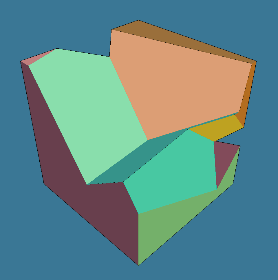
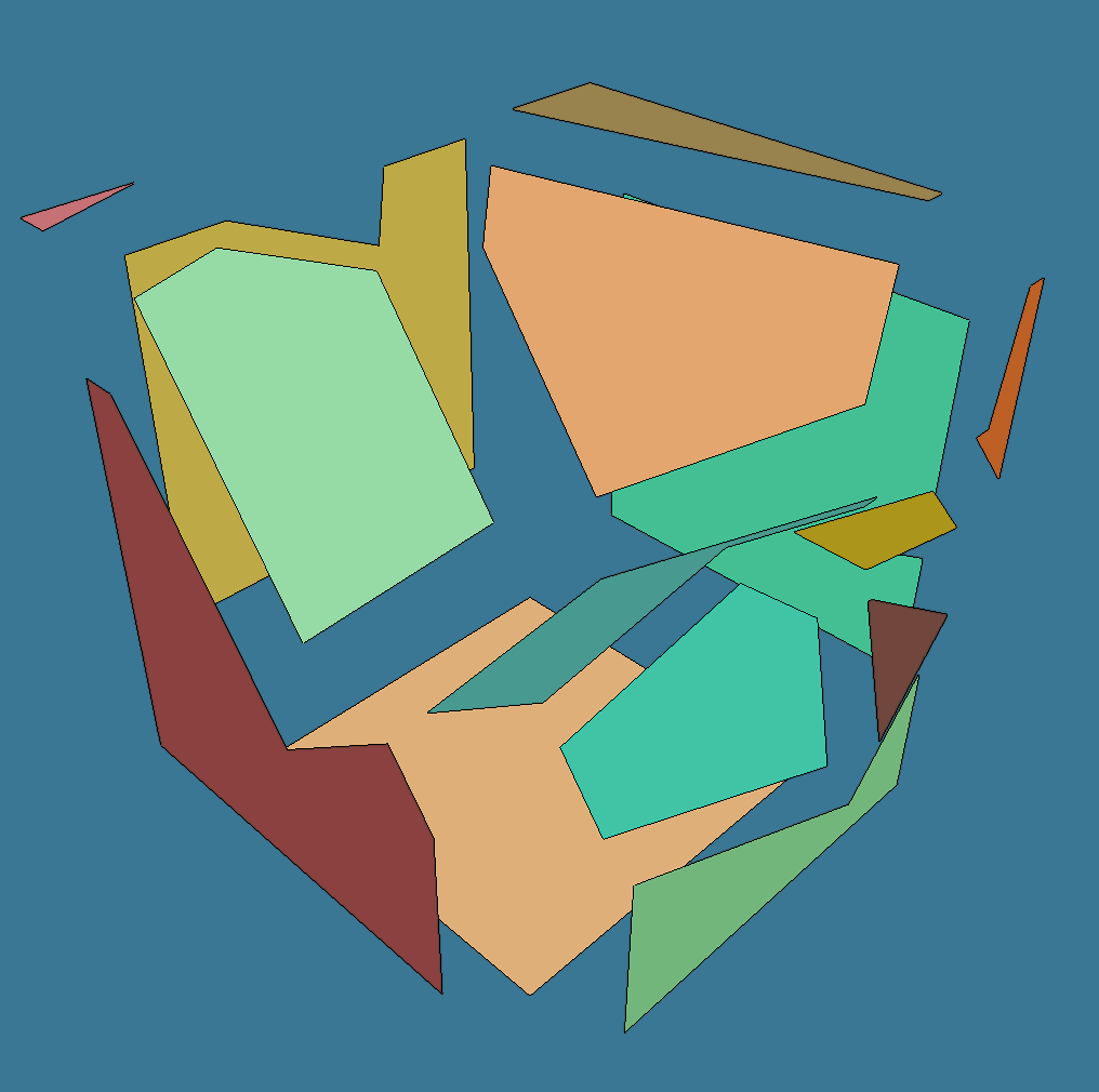
(a) (b) (c) (d) .

Figure 1: Boolean difference $(A\!\setminus\!B)\!\setminus\!C$ of three cubes, with 2-cells in different colors: (a) view from the front; (b) view from the back; (c) front with exploded 2-cells; (d) back with exploded 2-cells. Note that 2-cells of the resulting boundary may be non-convex.

Definition 3.6.3 (LAR Geometric Complex).

It is wortwhile to remark that, in order to display a triangulation of boundary faces in their proper position in space, the whole information required (geometry $+$ topology) is contained within the LAR Geometric Complex (GC):

$$\mu:C_{0}\to\mathbb{E}^{3},\ (\delta_{2},\delta_{1},\delta_{0})\qquad\equiv\qquad\texttt{(geometry, topology) = (W, (CF, FE, EV))}$$

A GC allows to transform the (possibly non connected) boundary 2-cycle of a Boolean result (see the example below) into a complete B-rep of the solid result. Note that ordered pairs of letters from V,E,F,C, correspond to the coboundary sequence Vertices$\to$Edges$\to$Faces$\to$Cells into the Column$\to$Row order of matrix maps of operators.

Remark (Chain representation).

Let us recall that CF (i.e., Faces${}\to{}$Cells) is the sparse matrix of coboundary operator $\delta_{2}:C_{2}\to C_{3}$, so that we have $[\partial_{3}]=[\delta_{2}]^{t}$, which in Julia is CF’. The value of AminBminC = .&(A,.!B,.!C) given in Example 3.6.6, is the $C_{2}$ representation of the oriented boundary 2-cycle of solid difference, displayed in Figure 1.

Note (From solid chains to B-reps).

Of course, the 14 non-zero elements in the boundary array (Example 3.6.6) of the AminBminC variable, correspond to the oriented boundary 2-cells of the solid result (see Example 3.6.6). Each of them is transformed into a possibly non connected 1-cycle by the FE’ sparse matrix, i.e., by the 2-boundary matrix $[\partial_{2}]=[\delta_{1}]^{t}$. Finally, every 1-cycle is transformed into one or more cyclic sequences of 0-cells, using the EV’ matrix, i.e., by using $[\partial_{1}]=[\delta_{0}]^{t}$. The indices of 0-cells are cyclically ordered, and used to generate sequences of 3D points via the embedding matrix W, which provides the vertex coordinates by column. This last step gives the ordered input for face triangulation using a CDT (Constrained Delaunay Triangulation) algorithm (Shewchuk, 2002) in 2D.

Property 3.6.2 (Storage space of LAR Geometric Complex).

The topology of a LAR 3-complex is fully represented by the operators $\delta_{0},\delta_{1},\delta_{2}$, i.e., by the sparse arrays (EV,FE,CF), providing the incidences between vertices, edges and faces, for both B-reps and decompositive representations. If a boundary representation is used, LAR storage is 3/4 of the good ancient winged-edge representation by Baumgart (1972), often used as storage comparison for solid modeling, and very close ($3\times 2E$, see Woo (1985)) to half-edge Muller and Preparata (1978), largely used in Computational Geometry.

Example 3.6.6.

Boundary of solid expression. The variable AminBminC contains the logical representation of the Boolean expression $(\texttt{A}\!\setminus\!\texttt{B})\!\setminus\!\texttt{C}$, specific to the particular algebra generated by terms in Example 3.6.1:

⬇

1julia> difference = Int8.(AminBminC)

28-element Array{Int8,1}:

3[0, 0, 0, 0, 1, 0, 0, 0]

4

5julia> boundary = CF’ * difference

647-element Array{Int8,1}:

7[1, 0, -1, 0, 0, 0, -1, 0, 1, 0, 1, 0, 0, 0, 1, -1, 0, -1, 0, -1, 0, 0, 1, 0, 0, 0, -1, 0, 0, 0, 0, 0, -1, 0, 0, 0, 0, 1, 0, 0, 0, 0, -1, 0, 0, 0, 0]

The value of the variable AminBminC is converted to the binary array difference—the coordinate representation of a 3-chain—by the vectorized constructor “$\texttt{Int8}.$”, in order to compute the boundary object of the Boolean expression which is shown in Figure 1, through multiplication times the boundary matrix $[\partial_{3}]\equiv\texttt{CF'}$ Finally, we note that in chain notation it is possible to write the following expression for the oriented boundary of the ternary solid Boolean difference. The actual reduction to triangulated boundary is obtained using FE’ and EV’ sparse matrices, and a constrained Delaunay triangulation (CDT) algorithm.

$$\texttt{boundary}\mapsto f_{A\backslash B\backslash C}=f_{1}-f_{3}-f_{7}+f_{9}+f_{11}+f_{15}-f_{16}-f_{18}-f_{20}+f_{23}-f_{27}-f_{33}+f_{38}-f_{43}$$

3.7 Boolean DSL

In this section we discuss the Domain Specific Language (DSL) design about the introduced Constructive Solid Geometry (CSG) algebra, as a Julia’s small set of macros, being currently under development.

Definition 3.7.1 (Functional form).

Let $\langle\mathcal{A};\otimes_{1},\ldots,\otimes_{k}\rangle$ be an algebra generated by $\mathcal{H}=\{h_{1},...,h_{m}\}$. A syntactic expression constructed as a valid sequence of operations $\otimes_{i}$ on $n$ variables $x_{i}$ denoting elements of $\mathcal{A}$ is called a functional form $\Phi$ over the algebra $\mathcal{A}$. Note that $\Phi(x_{1},...,x_{n})$ is not a function (is not a set of ordered pairs) but defines a function of $n$ arguments $\phi:\mathcal{A}^{n}\to\mathcal{A}.$

Remark (Evaluation process).

We use capital Greek letters such $\Phi,\Pi$, etc. to denote forms, and denote functions over algebras by lower case Greek letters. The distinction between forms and functions is important. Forms and functions over an algebra are formally related by an evaluation process, assigning values to the variables in the form, and computing the resulting value of the expression. This relationship is expressed by writing $\phi(x_{1},...,x_{n})=|\Phi(x_{1},...,x_{n})|.$

Property 3.7.1 (Evaluation process).

If $\mathcal{A}$ is a finite algebra, there is a finite number of distinct functions over $\mathcal{A}$, but an infinite number of distinct forms, e.g., strongly redundant. If $S\in\mathcal{A}$ is an element of the algebra generated by $\mathcal{H}$, there exists a form $\Phi$ over $\mathcal{A}$ such that: $S=|\Phi(\mathcal{H})|.$ We then say that $S$ is describable in $\mathcal{A}$ by $\mathcal{H}$. In general, $\Phi(\mathcal{H})$ is not unique, but $|\Phi(\mathcal{H})|$ is unique by definition.

Definition 3.7.2 (Domain Specific Language).

The Domain Specific Language (DSL) proposed in this paper for our CSG algebra is very simple. Its well-formed formulas are made by Julia identifiers of variables, Boolean operation symbols, and round brackets. A CSG expression is coded as a Julia macro @CSG, to provide a simpler interface to create Julia objects with complicated structure. The list of object models associated to variables is extracted by traversing the @CSG expression. Each object must be located and oriented in world coordinates using the Lar.Struct datatype, allowing to combine hierarchical assemblies (cellular complexes in local coordinates) and affine transformations. The application of the function Lar.struct2lar() evaluates a geometric object of type Lar.Struct, generating the triple (V,FV,EV), i.e., the LAR (DiCarlo et al., 2014) minimal models used by the CSG.jl package.

Algorithm 12 (Evaluation process).

The evaluation of a 3D Boolean functional form @CSG <expr>, into an evaluated LAR model (V,(CF,FE,EV)), made by a $3\times n$ array V and by a triple (CF,FE,EV) of sparse arrays, providing respectively the geometric embedding $C_{0}\to\mathbb{E}^{3}$, and a chain complex $\delta_{2},\delta_{1},\delta_{0}$, is made by several tasks:

1. Evaluation of data and functional forms. Input: a single @CSG macro block, possibly delimited by begin...end clause, including solid terms and (possibly) component @CSG clauses. Output: parse tree of compound @CSG expression; ordered tuple of variable names associated to input objects in a single coord frame: (A₁,$\ldots$,A_m).

2. Computation of space arrangement. Input: tuple of solid terms in world coordinates: (A₁,$\ldots$,A_m). Output: sparse boundary matrices (FC,EF,VE) as $[\partial_{3}],[\partial_{2}],[\partial_{1}]$, and (new) vertex matrix W. The columns of $[\partial_{3}]$ are ono-to-one with the atoms generating the @CSG algebra.

3. Evaluation of Boolean terms. Input: the boundary representation of atoms of CSG algebra, generated by chain complex (W,(FC,EF,VE)), and the input (A₁,$\ldots$,A_m) terms. Output: logical $n\times m$ array B = Array{Bool,2} whose column $\texttt{B}_{j}$ gives the bit array representing the A_j term of @CSG algebra input form.

4. Bitwise computing of Boolean function. Input: the logical array B; the parse tree of top-level @CSG expression. Output: a single BitArray of length $n$, as the number of Boolean atoms. The 1$s$ in this array denote the atomic 3-chains whose disjoint union produce the Boolean result, i.e., the value of evaluated @CSG form.

5. Boundary evaluation of output 3-chain. Input: the 3-chain (binary) coordinate representation of the Boolean result; the chain complex W,(FC,EF,VE). Output: the boundary representation of the Boolean result, possibly exported in a standard vector graphics format, like, e.g., the file formats .OBY, .PLY, or .DAE (Digital Asset Exchange — COLLADA XML). Our software prototype may currently export in 2D and 3D .OBY.

Definition 3.7.3 (Boolean form).

Clause (expression formed from a finite collection of literals) that matches other clauses and/or LAR models, by matching Boolean combinations of other clauses. It is built using one or more @CSG macro, each one with a typed “Struct” occurrence. The semantics of a Struct, natively including only “aggregation” and “affine transformation”, is enriched with $n$-ary union, intersection, difference, and complement symbols. Let $\texttt{A},\texttt{B},\texttt{C},\dots$ be either LAR models or Struct literals or values. We have:

:(+, A,B,C,...) $$\texttt{::= Struct}\left(\texttt{:union},\texttt{[A,B,C,...]}\right)$$

:(*, A,B,C,...) $$\texttt{::= Struct}\left(\texttt{:intersect},\texttt{[A,B,C,...]}\right)$$

:(-, A,B,C,...) $$\texttt{::= Struct}\left(\texttt{:diff},\texttt{[A,B,C,...]}\right)$$

4 Computational examples

This section provides the reader with some examples of solid modeling programming style with Julia and its sparse and non-sparse arrays. We believe that giving a look at a few simple concrete examples is useful for understanding our computational approach and its possible developments. Sections 4.1 and 4.2 aim at showing the sequence of spaces and transformations that finally produce a solid model when evaluating a Boolean expression through a function application Lar.bool3d(assembly). We show in Section 4.3 that the exactness property ($\partial^{2}=0$) of any chain complex can be used to check the accuracy of calculations. The Euler characteristic of the union solid model generated in Example 3.6.1 is stepwise computed in Section 4.4, where we use the chain maps $\partial_{3},\partial_{2},\partial_{1}$ to obtain the sets (and numbers) of faces, edges and vertices belonging to the boundary of the union solid, which is a closed 2-manifold of genus zero (see Figure 2). As we told before, a specific API and a mini DSL for CSG expressions are being planned.

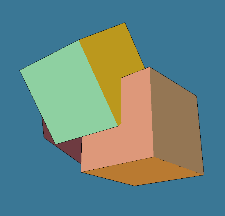
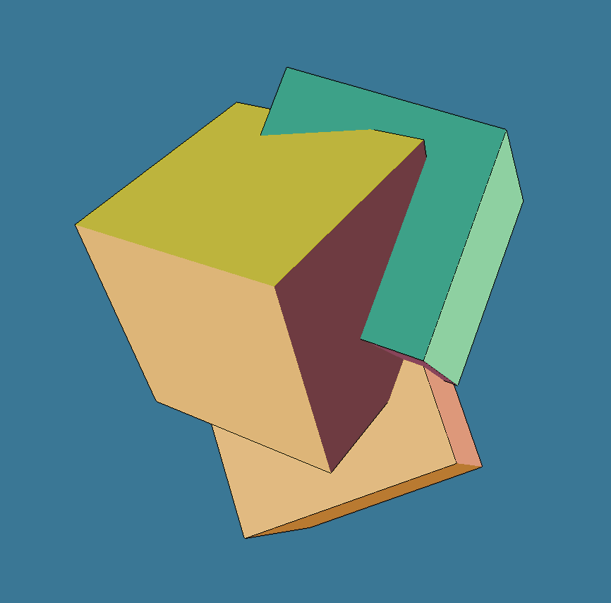
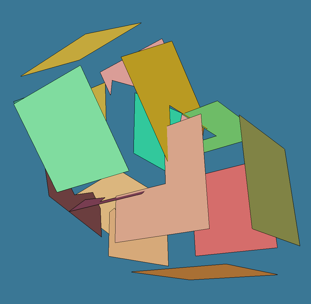
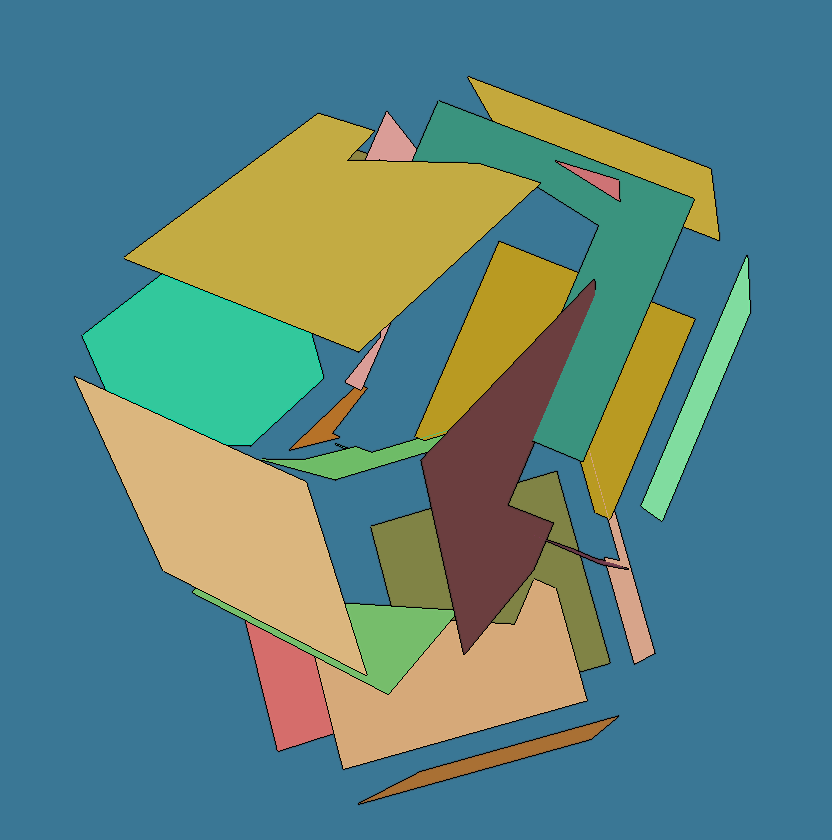
(a) (b) (c) (d) .

Figure 2: Boolean union $A\cup B\cup C$ of three cubes (from assembly of Example 3.6.1), with 2-cells in different colors: (a) view from the front; (b) view from the back; (c) front with exploded 2-cells; (d) back with exploded 2-cells. For clarity sake, only the boundary 2-cells are displayed. The space partition generated other 2-cells in the interior, of course.

4.1 Variadic union

In order to compute the union of three affinely transformed instances of the unit cube, we consider the assembly expression given in Example 3.6.1. First we get the $\mathbb{E}^{3}$ space partition and the term structure generated by assembly through the function Lar.bool3d; then we combine the logical arrays A, B, and C, building the value of BitArray type for the union variable, that stores the logical representation of the specific 3-chain. Let us remark that the bitwise “or” operator (“$|$”) is applied in a vectorized way to arrays, by inserting a dot character:

⬇

1julia> W, (EV, FE, CF), boolmatrix = Lar.bool3d(assembly);

2julia> A,B,C = boolmatrix[:,2],boolmatrix[:,3],boolmatrix[:,4]

3julia> union = .|(A, B, C);

4julia> @show union;

5

6union = Bool[false, true, true, true, true, true, true, true]

Finally, the boundary 2-cycle faces is generated by multiplication of the sparse matrix $[\partial_{3}]$ (i.e., CF’) times the binary converted union. The mapping Bool $\to\{0,1\}$ is applied via a vectorized application of the Int8 constructor:

⬇

1julia> faces = CF’ * Int8.(union);

2julia> @show faces;

3

4faces = [1, 0, -1, 0, 0, 0, -1, 0, 1, 0, 1, 0, 0, 0, 1, -1, 0, -1, 0, 0, 1, -1, 0, -1, 1,

50, 0, 0, 1, 1, 0, -1, 0, 0, 1, 0, -1, 0, 0, 0, -1, 1, 0, 1, 0, 0, -1]

With $f_{k}\in U_{2}$, where $U_{2}$ is the basis of chain space $C_{2}$ generated by $\mathcal{A}\,(\texttt{assembly})$, we may write in chain notation:

$$\begin{split}\small\texttt{faces}\mapsto f_{A\cup B\cup C}=&f_{1}-f_{3}-f_{7}+f_{9}+f_{11}+f_{15}-f_{16}-f_{18}+f_{21}-f_{22}-f_{24}\\ &+f_{25}+f_{29}+f_{30}-f_{32}+f_{35}-f_{37}-f_{41}+f_{42}+f_{44}-f_{47}\end{split}$$ (4)

The boundary representation, i.e., the subset of boundary’s oriented faces, is given by the 2-cycle in Eqation 5. They are transformed into a boundary triangulation, needed for graphic display, by proper use of $[\partial_{2}]=\texttt{FE'}$ and $[\partial_{1}]=\texttt{EV'}$.

4.2 Meaning of $\partial$ matrices

By definition, the matrix $[\partial_{2}]=\texttt{FE'}=\texttt{EF}$ contains by columns the $U_{2}$ basis expressed as an ordered sequence of 1-cycle vectors. Signed values provide cyclic ordering of 1-cycles of edges, easily extendible to higher dimensions. With $e_{h}\in U_{1}$, we have:

⬇

1FE’[:, 1] $\mapsto$ f₁ = e₁ -e₂ +e₄ -e₅ +e₆ -e₇ +e₈

2FE’[:, 2] $\mapsto$ f₂ = e₃ +e₇ -e₈

3... ... ...

4FE’[:,47] $\mapsto$ f₄₇ = e₆₄ -e₆₉ +e₇₇ -e₈₁ -e₈₆ +e₈₈

Each 1-cell $e_{h}$ is mapped to an ordered pair of 0-cells $v_{j}\in U_{0}$, via the boundary matrix $[\partial_{1}]=[\delta_{0}]^{t}=\texttt{EV'}$:

⬇

1EV’[:, 1] $\mapsto$ e₁ = v₂ - v₁

2EV’[:, 2] $\mapsto$ e₂ = v₆ - v₃

3... ... ...

4EV’[:,49] $\mapsto$ e₄₉ = v₂₉ - v₂₆

The geometric embedding in $\mathbb{E}^{3}$ of the $A\cup B\cup C$ model generated in Section 4.1 is provided by the coordinate array $\texttt{W}\in\mathbb{R}^{3}_{49}$, with 3 rows and 43 columns. The coordinate array V embedding the initial assembly model, consisting of three non (yet) intersected cubes, has instead dimension $3\times 24$.

4.3 Correctness checks

A computational approach based on chain complexes offers unique tools for checking the accuracy of calculations, that are correct by construction, since both $\partial^{2}=0$ and $\delta^{2}=0$ hold, when applied to any chain. In words, every boundary is a cycle, or equivalently: the chain complex is exact. Also, we know that the boundary of every solid is a possibly non-connected closed surface, hence a 2-cycle. This holds if and only if the construction of $[\partial]$ matrices is done correctly. In the following example, we start from the chain of boundary faces of Section 4.1.

⬇

1julia> pairs = [(f,sign) for (f,sign) in enumerate(copCF’ * Int8.(union)) if sign != 0];

2julia> faces = map(prod, pairs);

3julia> @show faces;

4faces = [1,-3,-7,9,11,15,-16,-18,21,-22,-24,25,29,30,-32,35,-37,-41,42,44,-47]

We obtain the following 2-chain as boundary 2-cycle. The cardinality of the faces array is $\chi_{2}=21$.

$$\begin{split}\texttt{\mbox{faces}}\mapsto f_{A\cup B\cup C}=&f_{1}-f_{3}-f_{7}+f_{9}+f_{11}+f_{15}-f_{16}-f_{18}+f_{21}-f_{22}-f_{24}+f_{25}+f_{29}+f_{30}\\ &-f_{32}+f_{35}-f_{37}-f_{41}+f_{42}+f_{44}-f_{47}\end{split}$$ (5)

The edge subset on the boundary of the union solid is computed by: (a) transforming the faces array of signed indices of 2-cells into the COORD representation (rows,cols,vals) of a sparse matrix (Cimrman, 2015); (b) holding a single boundary face (2-cell) per column in facemat; (c) multiplying this matrix times the $[\partial_{2}]$ operator, thus obtaining the new sparse matrix edges4face, holding a face 1-cycle per column; and, finally, (d) extracting only the positive instance of boundary edges belonging to the boundary faces. The number of boundary edges $\chi_{1}=57$ is one half of the non-zero terms in the sparse vector edges4face. The other half has the opposite sign, so that the total sum is zero:

⬇

1julia> nonzeros = hcat([[abs.(face),k,sign(face)] for (k,face) in enumerate(faces)]...);

2julia> facemat = sparse([nonzeros[k,:] for k=1:size(nonzeros,1)]...);

3julia> edges4face = copFE’ * facemat;

4julia> rows,cols,vals = findnz(edges4face);

⬇

1julia> edges = [e*sign for (e,sign) in zip(rows,vals) if sign==1];

2julia> @show edges;

3

4edges = [1,4,6,8,10,14,18,20,9,23,26,27,2,34,30,36,38,5,29,24,43,15,42,28,47,51,53,54,21,52,57,

5 48,61,62,64,50,59,66,55,58,40,63,68,77,79,80,35,78,83,72,88,7,74,87,69,81,86]

We remark again that, without filtering out the terms of negative sign, we would get an edges array of signed indices summing to zero, according to the constraint $\partial^{2}=0$. This attests to the exactness of calculations.

4.4 Euler characteristic

Euler characteristic of a solid of genus $g$ in $\mathbb{E}^{3}$ is defined as

$$\chi(g)=\chi_{0}-\chi_{1}+\chi_{2}=2-2g,$$

where $\chi_{0},\chi_{1},\chi_{2}$ are, respectively, equal to the number of vertices, edges and faces on the boundary of the solid. In our case, the number of boundary faces is $\chi_{2}=21$, according to Eq. (5). The edges indices given in Section 4.3 determine the 1-chain $e_{A\cup B\cup C}$ (or, more precisely, the non-independent 1-cycle generated by the independent 2-cycles of boundary faces). The cardinality of the edges array provides $\chi_{1}=57$. Note that, in order to counting the edges, we consider only the positive instances of 1-cells, since they appear in pairs (positive and negative) in a closed and coherently oriented cellular 2-complex.

$$\footnotesize\begin{split}\texttt{edges}\mapsto e_{A\cup B\cup C}&=e_{1}+e_{4}+e_{6}+e_{8}+e_{10}+e_{14}+e_{18}+e_{20}+e_{9}+e_{23}+e_{26}+e_{27}+e_{2}+e_{34}+e_{30}+e_{36}+e_{38}+e_{5}+e_{29}+e_{24}\\ &+e_{43}+e_{15}+e_{42}+e_{28}+e_{47}+e_{51}+e_{53}+e_{54}+e_{21}+e_{52}+e_{57}+e_{48}+e_{61}+e_{62}+e_{64}+e_{50}+e_{59}+e_{66}+e_{55}\\ &+e_{68}+e_{77}+e_{79}+e_{58}+e_{40}+e_{63}+e_{80}+e_{35}+e_{78}+e_{83}+e_{72}+e_{88}+e_{7}+e_{74}+e_{87}+e_{69}+e_{81}+e_{86}\end{split}$$ (6)

The final script computes the 0-chain $v_{A\cup B\cup C}$ of vertices on the boundary of union solid, with cardinality $\chi_{0}=38$.

⬇

1julia> nonzeros = hcat([[abs(e),k,sign(e)] for (k,e) in enumerate(edges)]...);

2julia> edgemat = sparse([nonzeros[k,:] for k=1:size(nonzeros,1)]...);

3julia> verts = sort(collect(Set(findnz(copEV’ * edgemat)[1])));

4julia> @show verts;

5verts = [1,2,3,4,5,6,7,8,9,10,12,15,17,18,19,20,21,24,25,26,27,30,31,32,33,34,

6 35,36,37,38,39,41,44,45,46,47,48,49]

In chain notation:

$$\footnotesize\begin{split}\texttt{verts}\mapsto v_{A\cup B\cup C}&=v_{1}+v_{2}+v_{3}+v_{4}+v_{5}+v_{6}+v_{7}+v_{8}+v_{9}+v_{10}+v_{12}+v_{15}+v_{17}+v_{18}+v_{19}+v_{20}+v_{21}+v_{24}+v_{25}+v_{26}\\ &+v_{27}+v_{30}+v_{31}+v_{32}+v_{33}+v_{34}+v_{35}+v_{36}+v_{37}+v_{38}+v_{39}+v_{41}+v_{44}+v_{45}+v_{46}+v_{47}+v_{48}+v_{49}\\[5.69054pt] \end{split}$$ (7)

The generated union solid model has topological genus $g=0$ (see Figure 2). Therefore, the test of correctness provided by checking the Euler characteristic via Eqs. (5), (6), and (7), gives the correct answer:

$$\chi(\texttt{union})=\chi_{0}-\chi_{1}+\chi_{2}=38-57+21=2$$

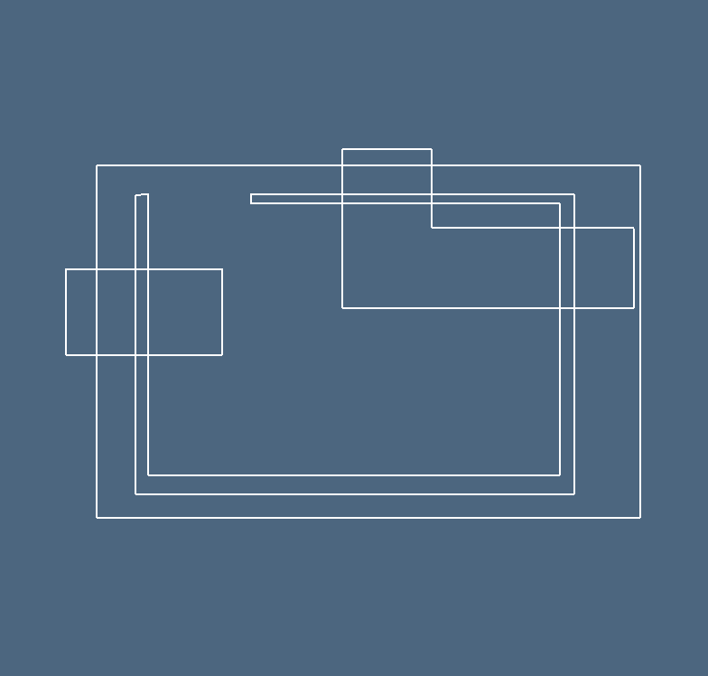
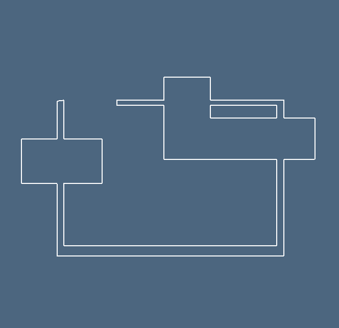
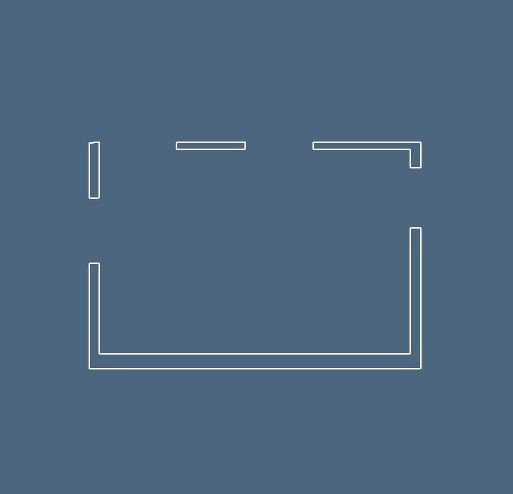
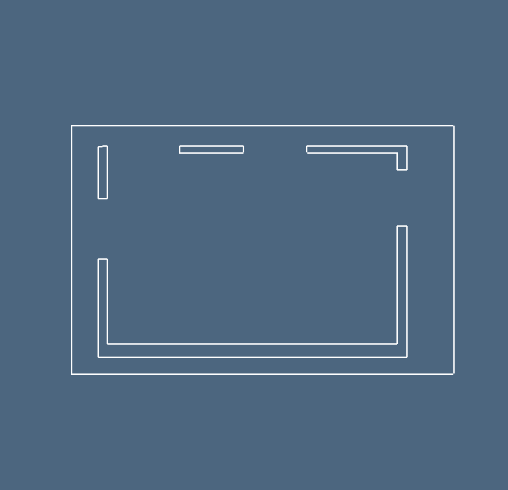
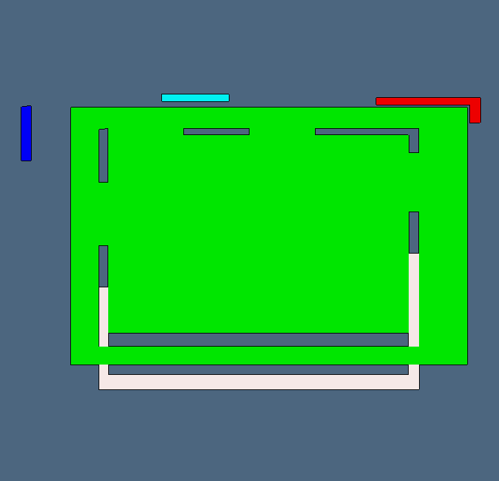
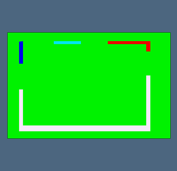
(a,b) (c,d) (e,f) (h,g) .

Figure 3: Some examples of variadic Booleans, obtained by applying the Boolean operators “.|”, “.-”, “.!”, and “.&” to the assembly variable, with 1-cells (B-reps) imported from SVG files. (a,b) start-to-end: from polygon input via SVG to (exploded) difference of outer box and interior walls; (c,d) boundary of union and union of some shapes; (e,f) difference 2-complex and its boundary; (g,h) boundary of outer box minus the previous 2-complex, and the corresponding 2-complex.

5 Result Discussion

The approach put forth in this paper is novel in several ways. First of all, we introduced here the first method of solid computational geometry, at authors’ knowledge, to assemble the terms of a CSG form using the atoms of a Boolean algebra, identified with the basis 3-chains of a partition of the embedding space, in turn given by the columns of the $[\partial_{3}]$ matrix in chain space. Furthermore, we initiated to set up the structure of Boolean form’s terms as binary arrays, aka coordinate vectors in $C_{3}$ space, and combining them by native bitwise operators. Moreover, with the only exception of $k$d-trees and interval-trees for acceleration of geometric queries, our approach does not use standard methods of computational geometry—in particular, of solid modeling subfield—which are based on highly specialized data structures, that are often very complex and require the implementation of very complicated algorithms.

We use instead basic tools and methods of linear algebra and algebraic topology, i.e., (sparse) matrices of linear operators and semiring matrix multiplication (Kepner et al., 2016), plus filtering. Hence, accuracy of topological computations is guaranteed by contruction, since operator matrices and chain bases, as well as any chain, satisfy the (graded) constraints $\partial^{2}=0$ and $\delta^{2}=0$, which are easy to check. Furthermore, we have shown that space and time complexities are comparable with those of traditional methods, and it is reasonable to expect that our approach might be extended to generic dimensions and/or implemented on highly parallel computational engines, using pretty standard and highly general computing libraries, e.g., GraphBLAS and GPU kernels. In this case a good speed-up is expected, given the high level of possible parallelization of our algorithms.

In this paper we have also given a new characterization of the computational process for evaluating CSG expressions of any depth and complexity. Traditional evaluation methods require a post-order DFS traversal of the expression tree, and the sequential computation of each Boolean operation encountered on nodes, until the root operation is evaluated. It is well known that such a process lacks in robustness and accumulates numerical errors, that ultimately modify the local topology and make the applications stop on error. Hence, intermediate boundary representations need to be generated and carefully curated, before continuing the traversal.

With our approach, the evaluation of a CSG expression of any complexity is done with a different computational process. A hierarchical structure of macros is used both to parse the expression tree and to apply affine transformations to solid primitives, in order to scale, rotate and translate them in their final (“world”) positions and attitudes. All their 2-cells are thus accumulated in a single collection, and each of them is independently fragmented, generating a collection of local topologies that are merged by boundary congruence, using a single round-off operation on vertices. The global space partition is so generated, and all input solids are classified with respect to 3-cells of this partition, i.e., the atomic objects of a Boolean algebra, with a single point-membership test per atom. Finally, any Boolean form of arbitrary complexity, with the same variables, can be quickly evaluated by bitwise vectorized logical operations.

Last but not least, all distinction is removed between manifold and non-manifold geometries, both in 2D and 3D, allowing for mixing B-reps and cellular decompositions of the interior of elementary solids. B-reps may be always generated for efficiency purposes—via boundary operator multiplication—in order to strongly reduce the number of 2-cells to be decomposed (possibly in parallel), but this is not strictly required. This flexibility about input data types could be useful, in particular, for combining outer surfaces with regular solid grids, and is consistent with the generation of internal structures to make 3D printed models more reliable and easy to produce.

Acknowledgements

Several people have contributed or are currently contributing to implement different parts and algorithms of this project, including Gianmaria DelMonte, Francesco Furiani, Giulio Martella, Elia Onofri, and Giorgio Scorzelli. Antonio Bottaro believed in this project and funded its development as responsible of R&D of Sogei (Italian Ministry of Economy and Finance) and CEO of the Geoweb subsidiary.

6 Conclusions and future prospects

We have introduced a novel approach to computation of Boolean operations between solid models. In particular, we have shown that any Boolean expression between solid models may be evaluated using the finite algebra associated with the set of independent generators of the chain space produced by the arrangement of Euclidean space generated by a collection of geometric objects. The computational approach to geometric design introduced by this paper is quite different from traditional methods of geometric modeling and computational geometry.

Two prototypes of open-source implementation were written in Julia language (Bezanson et al., 2017), mostly using sparse arrays. At the present time, we can only evaluate CSG formulas with closed regular cells. A novel implementation for closure algebras is planned, using the parallel and distribute features of Julia, that provides best-in-class support to linear algebra and matrix computations, including the new GraphBLAS (Kepner et al., 2016) standard.

We think that, by introducing linear methods in solid geometry, we have in some sense only scratched the surface of the new body of knowledge being currently investigated by machine learning methods for image understanding, that also use tensors and linear algebra. Next generation ML methods need formal and abstract techniques for building and merging solid models derived from partial images. We have already done some early experiments of our topological algebraic method in 3D medical imaging, by combining boundary and coboundary operators with filters, aiming at discovering and tracing complex interior structures. We hope that the techniques introduced by this paper may provide some basic tools for many applications in this and other fields.

References

- Arnold (2018) Arnold, D.N., 2018. Finite Element Exterior Calculus. volume 93 of CBMS-NSF Regional Conference Series in Applied Mathematics. Society for Industrial and Applied Mathematics (SIAM), Philadelphia, PA.
- Baumgart (1972) Baumgart, B.G., 1972. Winged edge polyhedron representation. Technical Report Stan-CS-320. Stanford, CA, USA.
- Bezanson et al. (2017) Bezanson, J., Edelman, A., Karpinski, S., Shah, V.B., 2017. Julia: A fresh approach to numerical computing. SIAM Review 59, 65–98. URL: http://julialang.org/publications/julia-fresh-approach-BEKS.pdf, doi:10.1137/141000671.
- Bieri (1995) Bieri, H., 1995. Nef polyhedra: A brief introduction, in: Hagen, H., Farin, G., Noltemeier, H. (Eds.), Geometric Modelling, Springer Vienna, Vienna. pp. 43–60.
- Björner and Ziegler (1992) Björner, A., Ziegler, G., 1992. Combinatorial stratification of complex arrangements. J. Amer. Math. Soc. , 105–149.
- Braid (1975) Braid, I.C., 1975. The synthesis of solids bounded by many faces. Commun. ACM 18, 209–216. URL: http://doi.acm.org/10.1145/360715.360727, doi:10.1145/360715.360727.
- Chew (1987) Chew, L.P., 1987. Constrained delaunay triangulations, in: Proceedings of the Third Annual Symposium on Computational Geometry, Association for Computing Machinery, New York, NY, USA. p. 215–222. URL: https://doi.org/10.1145/41958.41981, doi:10.1145/41958.41981.
- Cimrman (2015) Cimrman, R., 2015. Sparse matrices in scipy, in: Varoquaux, G., Gouillart, E., Vahtras, O., deBuyl, P. (Eds.), Scipy lecture notes. Zenodo. URL: https://scipy-lectures.org/advanced/scipy_sparse/index.html, doi:10.5281/zenodo.594102.
- Davis (2019) Davis, T.A., 2019. Algorithm 1000: Suitesparse:graphblas: Graph algorithms in the language of sparse linear algebra. ACM Trans. Math. Softw. 45. URL: https://doi.org/10.1145/3322125, doi:10.1145/3322125.
- DelMonte et al. (2020) DelMonte, G., Onofri, E., Scorzelli, G., Paoluzzi, A., 2020. Local congruence of chain complexes. arXiv e-prints , arXiv:2004.00046arXiv:2004.00046.
- DiCarlo et al. (2009a) DiCarlo, A., Milicchio, F., Paoluzzi, A., Shapiro, V., 2009a. Chain-based representations for solid and physical modeling. Automation Science and Engineering, IEEE Transactions on 6, 454 --467. doi:10.1109/TASE.2009.2021342.
- DiCarlo et al. (2009b) DiCarlo, A., Milicchio, F., Paoluzzi, A., Shapiro, V., 2009b. Discrete physics using metrized chains, in: 2009 SIAM/ACM Joint Conference on Geometric and Physical Modeling, Acm, New York, NY, USA. pp. 135--145. doi:10.1145/1629255.1629273.
- DiCarlo et al. (2014) DiCarlo, A., Paoluzzi, A., Shapiro, V., 2014. Linear algebraic representation for topological structures. Comput. Aided Des. 46, 269--274. URL: http://dx.doi.org/10.1016/j.cad.2013.08.044, doi:10.1016/j.cad.2013.08.044.
- Dimca (2017) Dimca, A., 2017. Hyperplane Arrangements: an Introduction. Springer. URL: https://www.springer.com/gp/book/9783319562209.
- Edelsbrunner (1987) Edelsbrunner, H., 1987. Algorithms in Combinatorial Geometry. Springer-Verlag New York, Inc., New York, NY, USA.
- Fabri et al. (2000) Fabri, A., Giezeman, G.J., Kettner, L., Schirra, S., Schönherr, S., 2000. On the design of cgal a computational geometry algorithms library. Softw. Pract. Exper. 30, 1167--1202. URL: http://dx.doi.org/10.1002/1097-024X(200009)30:11<1167::AID-SPE337>3.0.CO;2-B, doi:10.1002/1097-024X(200009)30:11<1167::AID-SPE337>3.0.CO;2-B.
- Fogel et al. (2007) Fogel, E., Halperin, D., Kettner, L., Teillaud, M., Wein, R., Wolpert, N., 2007. Arrangements, in: Boissonat, J.D., Teillaud, M. (Eds.), Effective Computational Geometry for Curves and Surfaces. Springer. Mathematics and Visualization. chapter 1, pp. 1--66.
- Goldwasser (1995) Goldwasser, M., 1995. An implementation for maintaining arrangements of polygons, in: Proceedings of the Eleventh Annual Symposium on Computational Geometry, Acm, New York, NY, USA. pp. 432--433. URL: http://doi.acm.org/10.1145/220279.220337.
- Goodman et al. (2017) Goodman, J.E., O’Rourke, J., Tòth, C.D. (Eds.), 2017. Handbook of Discrete and Computational Geometry -- Third Edition. CRC Press, Inc., Boca Raton, FL, USA.
- Hachenberger et al. (2007) Hachenberger, P., Kettner, L., Mehlhorn, K., 2007. Boolean operations on 3d selective nef complexes: Data structure, algorithms, optimized implementation and experiments. Comput. Geom. Theory Appl. 38, 64--99. URL: http://dx.doi.org/10.1016/j.comgeo.2006.11.009, doi:10.1016/j.comgeo.2006.11.009.
- Halmos (1963) Halmos, P., 1963. Lectures on Boolean Algebras. Van Nostrand.
- Halperin and Sharir (2017) Halperin, D., Sharir, M., 2017. Arrangements, in: Goodman, J.E., O’Rourke, J., Tòth, C.D. (Eds.), Handbook of Discrete and Computational Geometry -- Third Edition. CRC Press, Inc., Boca Raton, FL, USA. chapter 28.
- Hatcher (2002) Hatcher, A., 2002. Algebraic topology. Cambridge University Press.
- Hoffmann et al. (1987) Hoffmann, C.M., Hopcroft, J.E., Karasick, M.S., 1987. Robust Set Operations on Polyhedral Solids. Technical Report. Ithaca, NY, USA.
- Hoffmann and Shapiro (2017) Hoffmann, C.M., Shapiro, V., 2017. Solid modeling, in: Toth, C.D., O’Rourke, J., Goodman, J.E. (Eds.), Handbook of Discrete and Computational Geometry. Chapman and Hall/CRC. chapter 57. URL: https://doi.org/10.1201/9781315119601.
- Kasper and Arns (1993) Kasper, J.E., Arns, D., 1993. Graphics Programming with PHIGS and PHIGS PLUS. Hewlett-Packard/Addison-Wesley, Inc., Reading, MA, USA.
- Kepner et al. (2016) Kepner, J., Aaltonen, P., Bader, D.A., Buluç, A., Franchetti, F., Gilbert, J.R., Hutchison, D., Kumar, M., Lumsdaine, A., Meyerhenke, H., McMillan, S., Moreira, J.E., Owens, J.D., Yang, C., Zalewski, M., Mattson, T.G., 2016. Mathematical foundations of the graphblas. CoRR abs/1606.05790. URL: http://arxiv.org/abs/1606.05790, arXiv:1606.05790.
- Muller and Preparata (1978) Muller, D.E., Preparata, F.P., 1978. Finding the intersection of two convex polyhedra. Theoretical Computer Science 7, 217–236.
- Paoluzzi (2003) Paoluzzi, A., 2003. Geometric Programming for Computer Aided Design. John Wiley & Sons, Chichester, UK. URL: https://doi.org/10.1002/0470013885.
- Paoluzzi et al. (1989) Paoluzzi, A., Ramella, M., Santarelli, A., 1989. Boolean algebra over linear polyhedra. Comput. Aided Des. 21, 474--484. URL: http://dl.acm.org/citation.cfm?id=70248.70249.
- Paoluzzi et al. (2017a) Paoluzzi, A., Shapiro, V., DiCarlo, A., 2017a. Arrangements of cellular complexes. CoRR abs/1704.00142. URL: http://arxiv.org/abs/1704.00142, arXiv:1704.00142.
- Paoluzzi et al. (2017b) Paoluzzi, A., Shapiro, V., DiCarlo, A., Furiani, F., Martella, G., Scorzelli, G., 2017b. Topological computing of arrangements with (co)chains. ACM Transactions on Spatial Algorithms and Systems (Accepted for publication).
- Preparata and Shamos (1985) Preparata, F.P., Shamos, M.I., 1985. Computational Geometry: An Introduction. Springer-Verlag New York, Inc., New York, NY, USA.
- Requicha (1977) Requicha, A., 1977. Mathematical models of rigid solids, in: Tech. Memo28, Production Automation Project. University of Rochester.
- Requicha (1980) Requicha, A., 1980. Representations for rigid solids: Theory, methods and systems. ACM Computing Surveys 12, 437--464.
- Requicha and Tilove (1978) Requicha, A., Tilove, R., 1978. Mathematical foundations of constructive solid geometry: General topology of closed regular sets. Technical Report PAP Memorandum 23. The University of Rochester. Rochester, NY.
- Rossignac and O’Connor (1989) Rossignac, J.R., O’Connor, M.A., 1989. A dimension-Independent Model for Pointsets with Internal Structures and Incomplete Boundaries. Technical Report Research Report RC 14340. IBM Research Division. Yorktown Heights, N.Y. 10598.
- Rowland and Weisstein (2005) Rowland, T., Weisstein, E.W., 2005. Characteristic function, in: From MathWorld. A Wolfram Web Resource. URL: ttps://mathworld.wolfram.com/CharacteristicFunction.html.
- Shapiro (1991) Shapiro, V., 1991. Representations of Semi-algebraic Sets in Finite Algebras Generated by Space Decompositions. Ph.D. thesis. Ithaca, NY, USA.
- Shapiro and Vossler (1993) Shapiro, V., Vossler, D.L., 1993. Separation for boundary to csg conversion. ACM Trans. Graph. 12, 35–55. URL: https://doi.org/10.1145/169728.169723, doi:10.1145/169728.169723.
- Shewchuk (2002) Shewchuk, J.R., 2002. Delaunay refinement algorithms for triangular mesh generation. Computational Geometry 22, 21 -- 74. URL: http://www.sciencedirect.com/science/article/pii/S0925772101000475, doi:https://doi.org/10.1016/S0925-7721(01)00047-5.
- Stone (1936) Stone, M.H., 1936. The theory of representations for Boolean algebras. Trans. Am. Math. Soc. 40, 37--111. doi:10.2307/1989664.
- Strang (2019) Strang, G., 2019. Linear Algebra and Learning from Data. Wellesley--Cambridge Press. URL: http://math.mit.edu/~gs/learningfromdata/.
- Tilove (1980) Tilove, R.B., 1980. Set membership classification: A unified approach to geometric intersection problems. IEEE Trans. on Computer , 874--883.
- Voelcker and Requicha (1977) Voelcker, H.B., Requicha, A.A.G., 1977. Constructive solid geometry. Technical Report TM-25. Production Automation Project, Univ. of Rochester.
- Weiler (1986) Weiler, K.J., 1986. Topological structures for geometric modeling. Ph.D. thesis. Rensselaer Polytechnic Institute.
- Woo (1985) Woo, T., 1985. A combinatorial analysis of boundary data structure schemata. Computer Graphics & Applications, IEEE 5, 19--27.
- Zhou et al. (2016) Zhou, Q., Grinspun, E., Zorin, D., Jacobson, A., 2016. Mesh arrangements for solid geometry. ACM Trans. Graph. 35, 39:1--39:15. URL: http://doi.acm.org/10.1145/2897824.2925901, doi:10.1145/2897824.2925901.