On robust expansiveness for sectional hyperbolic attracting sets

Abstract.

We prove that sectional-hyperbolic attracting sets for $C^{1}$ vector fields are robustly expansive (under an open technical condition of strong dissipativeness for higher codimensional cases). This extends known results of expansiveness for singular-hyperbolic attractors in $3$-flows even in this low dimensional setting. We deduce a converse result taking advantage of recent progress in the study of star vector fields: a robustly transitive attractor is sectional-hyperbolic if, and only if, it is robustly expansive. In a low dimensional setting, we show that an attracting set of a $3$-flow is singular-hyperbolic if, and only if, it is robustly chaotic (robustly sensitive to initial conditions).

1. Introduction

The theory of uniformly hyperbolic dynamics was initiated in the 1960s by Smale [52] and, through the work of his students and collaborators, as well as mathematicians in the Russian school (e.g. [2, 3]), led to a great development of the field of dynamical systems. This elegant theory did not cover which turned out to be important classes of dynamical systems: the most influential examples being, arguably, the Hénon map [27], for the discrete time case; and the Lorenz flow [35], for the continuous time case.

To extend the notion of uniform hyperbolicity to encompass sets containing equilibria accumulated by recurrent orbits, a fundamental step was given by Morales, Pacifico, and Pujals in [38, 44]. There they proved that a robustly transitive invariant attractor of a $3$-dimensional flow that contains some equilibria must be singular hyperbolic, i.e., it admits an invariant splitting $E^{s}\oplus E^{cu}$ of the tangent bundle into a $1$-dimensional uniformly contracting sub-bundle and a $2$-dimensional volume-expanding sub-bundle.

The first examples of singular hyperbolic sets included the Lorenz attractor [35, 32] and its geometric models [25, 1, 26, 56], and the singular-horseshoe [31], besides the uniformly hyperbolic sets themselves. Many other examples have been found e.g. [45, 40, 39, 42]. For arbitrary dimensions this notion was extended first in [37] by Metzger and Morales, and the first concrete example provided by Bonatti, Pumariño and Viana in [19]. These are sectional-hyperbolic attractors, where now the splitting $E^{s}\oplus E^{cu}$ of the tangent bundle can have $d_{cu}=\dim E^{cu}\geq 2$, $d_{s}=\dim E^{s}\geq 1$ and the area along any $2$-subspace of $E^{cu}$ is uniformly expanded by the tangent map of the flow.

In the absence of equilibria, both singular-hyperbolic sets and sectional-hyperbolic sets are uniform hyperbolic. It is natural to try to understand the dynamical consequences of sectional hyperbolicity.

In [9] the authors prove that all singular-hyperbolic attractors are expansive, meaning, roughly, that any pair of orbits which remain close at all times must actually coincide. There are different notions of expansiveness and similar, as ”kinematic expansive” which are considered in [21] and [28] and explored in [34] and [16]; and also “rescaled expansivity” [55]. Here we focus on the one introduced by Komuro [29] to be compatible with the dynamics of the geometric Lorenz attractor.

Here, building on the work [9] and more recently [6, 7, 10], we extend the expansiveness property obtained in [9] from sectional-hyperbolic attractors to sectional-hyperbolic attracting sets, extending the previous result even in the $3$-dimensional case, avoiding the assumption of the existence of a dense regular orbit in the set.

Moreover, we show that sectional-hyperbolic attracting sets are $C^{1}$ robustly expansive: we can find uniform bounds on the distance between pairs of orbits for any given $C^{1}$ nearby vector field so that the orbits must coincide. When $d_{cu}>2$ we need to assume a strong dissipativity condition on the vector field in a neighborhood of the attracting set, which is still a $C^{1}$ open condition.

The main tool of the proof is the construction of a global Poincaré return map to a suitably chosen family of cross-sections of the flow near the attracting set, extending the constructions from [9, 7, 10] to any dimension $d_{cu}>2$.

We then explore some consequences of our results. It is well-known that expansiveness implies $h$-expansiveness (entropy expansiveness) [20] and then the semicontinuity of the entropy function ensuring the existence of equilibrium states for all continuous potentials. Recently [47] entropy-expansiveness has been proved more directly for sectional-hyperbolic sets and used to obtain several ergodic theoretical results.

In addition, robust expansiveness implies that the vector field is a star vector field, and this class has many important features. Building on recent work from Wen [24] together with Shi and Gan [51] we obtain partial converses of the main result. Namely, a robustly expansive non-singular vector field is uniformly hyperbolic; and a robustly transitive attractor is sectional-hyperbolic if, and only if, it is robustly expansive.

Moreover, for $3$-flows we equate robust expansiveness and robust sensitivity to initial conditions, which we denominate chaotic behavior, to obtain that an attracting set of a $3$-flow is singular-hyperbolic if, and only if, it is robustly chaotic. Robust expansivity is also useful to obtain stability of asymptotic sojourn times given by physical measures, as recently explored in [5].

2. Statement of the results

Let $M$ be a compact connected Riemannian manifold with dimension $\dim M=m$, induced distance $d$ and volume form ${\rm Leb}$. Let $\mathcal{X}^{r}(M)$, $r\geq 1$, be the set of $C^{r}$ vector fields on $M$ and denote by $\phi_{t}$ the flow generated by $G\in\mathcal{X}^{r}(M)$.

2.1. Sectional-hyperbolic attracting sets

An invariant set $\Lambda$ for the flow $\phi_{t}$ is a subset of $M$ which satisfies $\phi_{t}(\Lambda)=\Lambda$ for all $t\in{\mathbb{R}}$. Given a compact invariant set $\Lambda$ for $G\in\mathcal{X}^{r}(M)$, we say that $\Lambda$ is isolated if there exists an open set $U\supset\Lambda$ such that $\Lambda=\bigcap_{t\in{\mathbb{R}}}\operatorname{Closure}{\phi_{t}(U)}$. If $U$ can be chosen so that $\operatorname{Closure}{\phi_{t}(U)}\subset U$ for all $t>0$, then we say that $\Lambda$ is an attracting set and $U$ a trapping region (or isolated neighborhood) for $\Lambda=\Lambda_{G}(U)=\cap_{t>0}\operatorname{Closure}{\phi_{t}(U)}$.

For a compact invariant set $\Lambda$, we say that $\Lambda$ is partially hyperbolic if the tangent bundle over $\Lambda$ can be written as a continuous $D\phi_{t}$-invariant sum $T_{\Lambda}M=E^{s}\oplus E^{cu},$ where $d_{s}=\dim E^{s}_{x}\geq 1$ and $d_{cu}=\dim E^{cu}_{x}\geq 2$ for $x\in\Lambda$, and there exist constants $C>0$, $\lambda\in(0,1)$ such that for all $x\in\Lambda$, $t\geq 0$, we have

• uniform contraction along $E^{s}$: $\|D\phi_{t}|E^{s}_{x}\|\leq C\lambda^{t};$ and

• domination of the splitting: $\|D\phi_{t}|E^{s}_{x}\|\cdot\|D\phi_{-t}|E^{cu}_{\phi_{t}x}\|\leq C\lambda^{t}.$

We say that $E^{s}$ is the stable bundle and $E^{cu}$ the center-unstable bundle. A partially hyperbolic attracting set is a partially hyperbolic set that is also an attracting set.

We say that the center-unstable bundle $E^{cu}$ is volume expanding if there exists $K,\theta>0$ such that $|\det(D\phi_{t}|E^{cu}_{x})|\geq Ke^{\theta t}$ for all $x\in\Lambda$, $t\geq 0$. More generally, $E^{cu}$ is sectional expanding if for every two-dimensional subspace $P_{x}\subset E^{cu}_{x}$,

$$|\det(D\phi_{t}(x)\mid P_{x})|\geq Ke^{\theta t}\quad\text{for all $x\in\Lambda$, $t\geq 0$}.$$ (2.1)

If $\sigma\in M$ and $G(\sigma)=0$, then $\sigma$ is called an equilibrium or singularity in what follows and we denote by $\operatorname{Sing}(G)$ the family of all such points. We say that a singularity $\sigma\in\operatorname{Sing}(G)$ is hyperbolic if all the eigenvalues of $DG(\sigma)$ have non-zero real part.

A point $p\in M$ is periodic for the flow $\phi_{t}$ generated by $G$ if $G(p)\neq\vec{0}$ and there exists $\tau>0$ so that $\phi_{\tau}(p)=p$; its orbit $\mathcal{O}_{G}(p)=\phi_{{\mathbb{R}}}(p)=\phi_{[0,\tau]}(p)$ is a periodic orbit, an invariant simple closed curve for the flow. The family of periodic orbits of $G$ is written $\operatorname{Per}(G)$.

The critical elements $\operatorname{Crit}(G)$ of a vector field $G$ are its equilibria and periodic orbits, that is, $\operatorname{Crit}(G)=\operatorname{Sing}(G)\cup\operatorname{Per}(G)$. An invariant set is nontrivial if it is not a critical element of the vector field.

We say that a compact invariant set $\Lambda$ is a sectional hyperbolic set if $\Lambda$ is partially hyperbolic with sectional expanding center-unstable bundle and all equilibria in $\Lambda$ are hyperbolic. A singular hyperbolic set which is also an attracting set is called a sectional hyperbolic attracting set.

A singular hyperbolic set is a compact invariant set $\Lambda$ which is partially hyperbolic with volume expanding center-unstable subbundle and all equilibria within the set are hyperbolic. A sectional hyperbolic set is singular hyperbolic and both notions coincide if, and only if, $d_{cu}=2$.

A sectional hyperbolic set with no equilibria is necessarily a hyperbolic set, that is, the central unstable subbundle admits a splitting $E^{cu}_{x}={\mathbb{R}}\{G(x)\}\oplus E^{u}_{x}$ for all $x\in\Lambda$ where $E^{u}_{x}$ is uniformly contracting under the time reversed flow; see e.g. [8]. That is, $\Lambda$ is a hyperbolic set if by definition $T_{\Lambda}M=E^{s}\oplus{\mathbb{R}}\{G\}\oplus E^{u}$.

A periodic orbit $\mathcal{O}_{G}(p)$ is hyperbolic if $\mathcal{O}_{G}(p)$ is a hyperbolic subset for $G$. If moreover $E^{u}$ is trivial (i.e. $E^{u}_{q}=\{\vec{0}\},q\in\mathcal{O}_{G}(p)$), then the periodic orbit is a periodic sink.

A singular hyperbolic attracting set cannot contain isolated periodic orbits. For otherwise such orbit must be a periodic sink, contradicting volume expansion.

We recall that a subset $\Lambda\subset M$ is transitive if it has a full dense orbit, that is, there exists $x\in\Lambda$ such that $\operatorname{Closure}{\{\phi_{t}x:t\geq 0\}}=\Lambda=\operatorname{Closure}{\{\phi_{t}x:t\leq 0\}}$.

A nontrivial transitive sectional hyperbolic attracting set is a sectional hyperbolic attractor.

The prototype of a sectional-hyperbolic attractor for $3$-flows is the Lorenz attractor; see e.g. [35, 53, 8]. For higher dimensional flows we have the multidimensional Lorenz attractor: see [19]. More examples are indicated in Remarks 2.1 and 3.2 and many more in[42].

2.2. Robust expansiveness for codimension-two sectional-hyperbolic attracting sets

The flow is sensitive to initial conditions if there is $\delta>0$ such that, for any $x\in M$ and any neighborhood $N$ of $x$, there is $y\in N$ and $t\in{\mathbb{R}}$ such that $d(\phi_{t}(x),\phi_{t}(y))>\delta$. We shall work with a much stronger property.

Definition 1.

Denote by $S({\mathbb{R}})$ the set of surjective increasing continuous functions $h:{\mathbb{R}}\to{\mathbb{R}}$. We say that the flow is expansive if for every $\varepsilon>0$ there is $\delta>0$ such that, for any $h\in S({\mathbb{R}})$

$$d(\phi_{t}(x),\phi_{h(t)}(y))\leq\delta,\quad\forall t\in{\mathbb{R}}\implies\exists t_{0}\in{\mathbb{R}}\text{ such that }\phi_{h(t_{0})}(y)\in\phi_{[t_{0}-\varepsilon,t_{0}+\varepsilon]}(x).$$

We say that a invariant compact set $\Lambda$ is expansive if the restriction of $\phi_{t}$ to $\Lambda$ is an expansive flow.

This notion was proposed by Komuro in [30]. We consider a robust version.

Definition 2.

We say that the vector field $G$ is robustly expansive on an attracting set $\Lambda=\cap_{t>0}\overline{\phi_{t}(U})$ if there exists a neighborhood $\mathcal{V}$ of $G$ in $\mathcal{X}^{1}(M)$ such that for every $\varepsilon>0$ there is $\delta>0$ such that, for any $x,y\in\Lambda_{Y}=\Lambda_{Y}(U)=\cap_{t>0}\overline{\psi_{t}(U)}$, $h\in S({\mathbb{R}})$ and $Y\in\mathcal{V}$

$$d(\psi_{t}(x),\psi_{h(t)}(y))\leq\delta,\quad\forall t\in{\mathbb{R}}\implies\exists t_{0}\in{\mathbb{R}}\text{ such that }\psi_{h(t_{0})}(y)\in\psi_{[t_{0}-\varepsilon,t_{0}+\varepsilon]}(x)$$

where $\psi_{t}$ is the flow generated by $Y$.

Our results show that a sectional hyperbolic attracting set $\Lambda$ is robustly expansive.

Theorem A.

Every sectional hyperbolic attracting set of a vector field $G\in\mathcal{X}^{1}(M)$, with $d_{cu}=2$, is $C^{1}$ robustly expansive.

2.3. Robust expansiveness for higher codimension

In the higher condimension case $d_{cu}>2$, we need to assume that $\Lambda$ satisfies a “strongly dissipative” condition, which is equivalent to a bunching condition on the partially hyperbolic splitting, but simpler to check for flows induced by vector fields. We implicitly assume without loss of generality that the compact manifold $M$ is embedded in an Euclidian space to simplifiy the statement of this condition.

Definition 3.

Let us fix $q>1/d_{s}$. We say that a partially hyperbolic attracting set $\Lambda$ is $q$-strongly dissipative if

• for every equilibria $\sigma\in\Lambda$ (if any), the eigenvalues $\lambda_{j}$ of $DG(\sigma)$, ordered so that $\Re\lambda_{1}\leq\Re\lambda_{2}\leq\cdots\leq\Re\lambda_{d}$, satisfy $\Re(\lambda_{1}-\lambda_{d_{s}+1}+q\lambda_{d})<0$;

• $\sup_{x\in\Lambda}\{\operatorname{div}G(x)+(d_{s}q-1)\|(DG)(x)\|_{2}\}<0$, where $\|\cdot\|_{2}$ denotes the matricial norm given by $\|A\|_{2}=(\Sigma_{ij}a^{2}_{ij})^{\frac{1}{2}}$ for a matrix $A_{d\times d}$.

This condition was introduced in [6] where it was shown to imply that the stable foliation associated to the partial hyperbolic attracting set extends to a $C^{1}$-smooth topological foliation of the basin of attraction of $\Lambda$.

Theorem B.

Every sectional hyperbolic attracting set of $1$-strongly dissipative vector field $G\in\mathcal{X}^{1}(M)$ is $C^{1}$ robustly expansive.

Remark 2.1.

The multidimensional Lorenz class of examples introduced in [19] provides classes of sectional-hyperbolic attractors for each choice of $d_{cu}\geq 2$ and $d_{s}\geq 2$; and also an example with $d_{cu}=3$ and $d_{s}=1$. There are plenty of singular-hyperbolic examples: see e.g. [42] and references therein.

In the the cases $d_{s}=1$ with $d_{cu}>2$ the $1$-strongly dissipative assumption is interpreted to mean “$q$-strongly dissipative for some $q>1$”.

Since we need the strong dissipativeness condition for technical reasons, we naturally pose the following.

Conjecture 1.

Theorem B is still true for all $C^{1}$ vector fields exhibiting a sectional hyperbolic attracting set.

2.4. Some consequences of robust expansiveness

We in fact obtain a slightly stronger result: the main argument provides a proof of (robust) positive expansiveness, that is, sectional-hyperbolic attracting sets in the setting of Theorems A and B satisfy: for each $\varepsilon>0$ we can find $\delta>0$ so that

$$d(\phi_{t}(x),\phi_{h(t)}(y))\leq\delta,h\in S({\mathbb{R}}),\forall t>0\implies\exists t_{0}>0,s\in(-\varepsilon,\varepsilon):\phi_{h(t_{0})}(y)\in{\mathcal{W}}^{s}_{\phi_{t_{0}+s}(x)};$$

where ${\mathcal{W}}^{s}_{z}$ is the local stable manifold through points $z\in U_{0}$, which are well-defined for partially hyperbolic attracting sets; see Section 3. We note that a slightly stronger notion of positive expansiveness (akin to Bowen-Walters expansiveness) has been shown in [15] to imply finitely many periodic orbits only.

From positive expansiveness, provided by Theorem 4.3, robust expansiveness follows as explained in Section 4.1, exploring the properties of stable manifolds of partially hyperbolic sets.

This enable us to obtain partial converses to the statements of the main Theorems A and B extending the results of [43] by (roughly) reinforcing robust transitivity with robust expansiveness.

We need the following standard notion. Given $G\in\mathcal{X}^{1}(M)$ and $x\in M$ we denote the omega-limit set

$$\omega(x)=\omega_{G}(x)=\left\{y\in M:\exists t_{n}\nearrow\infty\text{ s.t. }\phi_{t_{n}}x\xrightarrow[n\to\infty]{}y\right\}$$

and the alpha-limit set $\alpha(x)=\omega_{-G}(x)$, which are both non-empty on a compact ambient space $M$.

2.4.1. Robust expansive flows are star flows

A vector field $G\in\mathcal{X}^{1}(M)$ is a star vector field if there exists a $C^{1}$ neighborhood $\mathcal{U}$ of $G$ such that every critical element of every $Y\in\mathcal{U}$ is hyperbolic. The set of $C^{1}$ star vector fields of $M$ is denoted by $\mathcal{X}^{*}(M)$. The following is an extension of [46] to robust expansive flows in the sense of Komuro which encompasses singular flows; see e.g. [29, 9]. A proof of this can be found e.g. in [50, Theorem A].

Theorem 2.2.

A robustly expansive vector field $G\in\mathcal{X}^{1}(M)$ is a star vector field: $G\in\mathcal{X}^{*}(M)$.

Moreover, if $G\in\mathcal{X}^{1}(M)$ is robustly expansive on the attracting set $\Lambda_{X}(U)$ with trapping region $U$, then $G$ is a star vector field in $U$: there exists a neighborhood $\mathcal{U}\subset\mathcal{X}^{1}(M)$ of $G$ such that all critical elements of each $Y\in\mathcal{U}$ contained in $U$ are hyperbolic.

This is a very strong condition for non-singular vector fields: putting the last result together with [24] we obtain that every robustly expansive non-singular vector field $G$ is an Axiom A vector field satisfying the no-cycles condition.

2.4.2. Robustly transitive and expansive attractors are sectional-hyperbolic

Using the recent developments in the study of singular star flows from [51] we are able to prove the following. We say that an attractor $\Lambda_{G}(U_{0})$ is robustly transitive if there exists a $C^{1}$ neighborhood $\mathcal{U}\subset\mathcal{X}^{1}(M)$ such that $\Lambda_{Y}(U_{0})$ is transitive for all $Y\in\mathcal{U}$.

Corollary C.

Every robustly transitive and expansive attractor of $G\in\mathcal{X}^{1}(M)$ is sectional-hyperbolic.

In particular, every robustly transitive attractor of a star vector field is sectional-hyperbolic.

Remark 2.3.

Although robust transitivity of an attracting set alone implies sectional-hyperbolicity for $3$-flows, which is the main result of [44], this is not enough to ensure sectional-hyperbolicity for $m$-dimensional flows with $m\geq 4$. Indeed, the “wild strange attractor” presented by Shilnikov and Turaev in [54] is a robustly transitive singular attractor which is not sectional hyperbolic; see e.g. [37, Corollary 4.3] and [54, Lemma 4.2 and Theorem 4].

Remark 2.4.

Sectional-hyperbolicity for attracting sets of vector fields of class $C^{1+\varepsilon}$, for any given fixed $\varepsilon>0$, implies some strong ergodic properties: existence of physical/SRB measures whose basins cover a full Lebesgue measure subset of the trapping region [9, 10, 33, 4]; and these measures are rapid mixing and satisfy the Almost Sure Invariance Principle (which implies many other statistical properties: Central Limit Theorem, Law of the Iterated Logarithm etc) on an open and dense subset of such vector fields [7]. Since $\mathcal{X}^{2}(M)$ is $C^{1}$ dense in $\mathcal{X}^{1}(M)$ with the $C^{1}$ topology, all these results hold for a dense subset of the $C^{1}$ open classes and, naturally, also for $C^{2}$ open classes of such vector fields in Corollary C.

Coupling Corollary C with Theorem B we obtain a partial converse to this theorem.

Corollary D.

If $G\in\mathcal{X}^{1}(M)$ admits a robustly transitive attractor $\Lambda=\Lambda_{G}(U_{0})$ with trapping region $U_{0}$ where $G$ is $1$-strongly dissipative, then

$$\Lambda\text{ is sectional-hyperbolic }\iff\Lambda\text{ is robustly expansive.}$$

In [51] the authors show that $C^{1}$ generically among star vector fields $G$ on $4$-manifolds every Lyapunov stable chain recurrence class is sectional-hyperbolic, either for $G$ or for $-G$.

If $\dim M\geq 5$ there are transitive star flows with singularities of different indices [22]. For higher dimensional results we may additionally assume homogeneity; see the next subsection.

For conservative flows it is known that $C^{1}$ stably expansive conservative flows are Anosov, that is, globally hyperbolic; see e.g. [18].

2.4.3. Robust chaoticity and sectional-hyperbolicity

Recall that an invariant attracting subset $\Lambda$ is sensitive to initial conditions if, for every small enough $r>0$ and $x\in\Lambda$, and for any neighborhood $U$ of $x$, there exists $y\in U$ and $t\neq 0$ such that $\phi_{t}y$ and $\phi_{t}x$ are $r$-apart from each other: $d\big{(}\phi_{t}y,\phi_{t}x\big{)}\geq r$.

We say that an invariant subset $\Lambda$ for a flow $\phi_{t}$ is future chaotic with constant $r>0$ if, for every $x\in\Lambda$ and each neighborhood $U$ of $x$ in the ambient manifold, there exists $y\in U$ and $t>0$ such that $d\big{(}\phi_{t}y,\phi_{t}x\big{)}\geq r$. Analogously, we say that $\Lambda$ is past chaotic with constant $r$ if $\Lambda$ is future chaotic with constant $r$ for the reverse flow $\phi_{-t}$ (i.e., generated by $-G$).

If we have such sensitive dependence both for the past and for the future, we say that $\Lambda$ is chaotic. Note that sensitive dependence on initial conditions is weaker than chaotic, future chaotic or past chaotic conditions.

Clearly, expansiveness implies sensitive dependence on initial conditions. An argument with the same flavor as the proof of expansiveness provides the following (see also [12] for a different approach to sensitiveness).

Corollary E.

A sectional-hyperbolic attracting set $\Lambda=\Lambda_{G}(U)$ is robustly chaotic, i.e. there exists a neighborhood ${\mathcal{U}}$ of $G$ in $\mathcal{X}^{1}(M)$ and a constant $r_{0}>0$ such that $\Lambda_{Y}(U)=\cap_{t>0}\operatorname{Closure}{\psi_{t}(U)}$ is chaotic with constant $r_{0}$ for each $Y\in{\mathcal{U}}$, where $U$ is a trapping region for $\Lambda$ and $\psi_{t}$ is the flow generated by $Y$.

For a partially hyperbolic attracting set of codimension two we obtain a converse to Theorem A.

Corollary F.

Let $\Lambda$ be a partially hyperbolic attracting set for $G\in\mathcal{X}^{1}(M)$ with $d_{cu}=2$. Then $\Lambda$ is sectional-hyperbolic if, and only if, $\Lambda$ is robustly chaotic.

In the three-dimensional case we obtain the converse to Theorem A.

Corollary G.

Let $\Lambda$ be an attracting set for $G\in\mathcal{X}^{1}(M^{3})$. Then $\Lambda$ is sectional-hyperbolic if, and only if, $\Lambda$ is robustly chaotic.

Hence, robustly chaotic singular-attracting sets are necessarily Lorenz-like. Thus, if we can show that arbitrarily close orbits, in a small neighborhood of an attracting set, are driven apart, for the future as well as for the past, by the evolution of the system, and this behavior persists for all $C^{1}$ nearby three-dimensional vector fields, then the attracting set is sectional-hyperbolic.

We can extend this conclusion to higher dimensions assuming a stronger condition.

We say that a singularity $\sigma$ is generalized Lorenz-like if $DG(\sigma)|E^{cu}_{\sigma}$ has a real eigenvalue $\lambda^{s}$ and $\lambda^{u}=\inf\{\Re(\lambda):\lambda\in\operatorname{sp}(DG(\sigma)),\Re(\lambda)\geq 0\}$ satisfies $-\lambda^{u}<\lambda^{s}<0<\lambda^{u}$ (so the index of $\sigma$ is $\dim E^{s}_{\sigma}=d_{s}+1$). We say that $G$ is a robustly homogeneous vector field on the trapping region $U$ if, for some integer $1\leq i+1<m$ and for each vector field $Y$ in a $C^{1}$ neighborhood $\mathcal{U}$ of $G$:

• the singularities in $U$ are generalized Lorenz-like with index $i$ or $i+1$; and

• periodic orbits in $U$ are hyperbolic of saddle-type with the same index $i$.

Note that homogeneity is stronger than the star condition since the latter admits the coexistence of critical elements with arbitrary indices.

The following was already essentially obtained by Metzger and Morales in [37]; see Section 5 for a proof.

Theorem 2.5.

Let $\Lambda=\Lambda_{G}(U)$ be an attracting set for $G\in\mathcal{X}^{1}(M)$. If $G$ is robustly homogeneous in $U$, then $\Lambda$ is sectional-hyperbolic.

This result is also a tool needed to prove Corollaries F and G.

2.5. Organization of the text

We present preliminary results on sectional-hyperbolic attracting sets in Section 3 which are needed for the proofs of Theorems A and B, to be presented in Section 4.

In Section 5 we present an overview of the proof of Theorem 2.5 and, using this result as a tool together with all the previous results, we prove Corollary C in Subsection 5.3; and Corollaries E, F and G in Subsection 5.4.

Acknowledgements

This is based on the PhD thesis of J. Cerqueira at the Instituto de Matematica e Estatistica-Universidade Federal da Bahia (UFBA) under a CAPES/FAPESB scholarship. J. C. thanks the Mathematics and Statistics Institute at UFBA for the use of its facilities and the financial support from CAPES and FAPESB during his M.Sc. and Ph.D. studies. We thank A. Castro; V. Pinheiro; L. Salgado and F. Santos for many comments and suggestions which greatly improved the text. The authors also thank the anonymous referees for the careful reading and the many useful suggestions that greatly helped to improve the quality of the text.

3. Preliminary results on sectional-hyperbolic attracting sets

Let $G$ be a $C^{1}$ vector field admitting a singular-hyperbolic attracting set $\Lambda$ with isolating neighborhood $U$.

3.1. Generalized Lorenz-like singularities

We recall some properties of sectional-hyperbolic attracting sets extending some results from [6, 7] which hold for $d_{cu}\geq 2$.

Proposition 3.1.

Let $\Lambda$ be a sectional hyperbolic attracting set and let $\sigma\in\Lambda$ be an equilibrium. If there exists $x\in\Lambda\setminus\{\sigma\}$ so that $\sigma\in\omega(x)$, then $\sigma$ is generalized Lorenz-like.

Remark 3.2.

1. If $\sigma\in\operatorname{Sing}(G)\cap\Lambda$ is generalized Lorenz-like, then at $w\in\gamma_{\sigma}^{s}\setminus\{\sigma\}$ we have $T_{w}\gamma_{\sigma}^{s}=E^{cs}_{w}=E^{s}_{w}\oplus{\mathbb{R}}\cdot\{G(w)\}$ since $T\gamma_{\sigma}^{s}$ is $D\phi_{t}$-invariant and contains $G(w)$ (because $\gamma_{\sigma}^{s}$ is $\phi_{t}$-invariant) and the dimensions coincide.

2. If an equilibrium $\sigma\in\operatorname{Sing}(G)\cap\Lambda$ is not generalized Lorenz-like, then $\sigma$ is not in the positive limit set of $\Lambda\setminus\{\sigma\}$, i.e. there is no $x\in\Lambda\setminus\{\sigma\}$ so that $\sigma\in\omega(x)$. Moreover, we have $\dim E^{s}_{\sigma}\in\{d_{s},d_{s}+1\}$. An example is provided by the pair of equilibria of the Lorenz system of equations away from the origin: these are saddles with an expanding complex eigenvalue which belong to the attracting set of the trapping ellipsoid already known to E. Lorenz; see e.g. [8, Section 3.3] and references therein.

3. There are many examples of singular-hyperbolic attracting sets, non-transitive and containing non-Lorenz-like (generalized) singularities; see Figure 1 for an example obtained by conveniently modifying the geometric Lorenz construction, and many others in [42] or more recently in [17].

4. In what follows, a singular-hyperbolic attracting set with no (generalized) Lorenz-like singularities can be treated as non-singular attracting set, since non-Lorenz-like singularites do not interfere with the asymptotic dynamics of positive trajectories of points in the set.

5. There are examples of three-dimensional singular attractors with non-Lorenz-like singularities, but these sets are not robustly transitive and cannot be sectional-hyperbolic; see e.g. [41].

6. A singular hyperbolic attracting set contains no isolated periodic orbits. For such a periodic orbit would have to be a periodic sink, violating volume expansion.

Figure 1. Example of a singular-hyperbolic attracting set, non-transitive (in fact, it is the union of two transitive sets indicated by $H_{1},H_{2}$ above) and containing non-Lorenz like singularities.

Proof of Proposition 3.1.

It follows from sectional-hyperbolicity that $\sigma$ is a hyperbolic saddle and that at most $d_{cu}$ eigenvalues have positive real part. If there are only $d_{cu}-1$ such eigenvalues, then the constraints on $\lambda^{s}$ and $\lambda^{u}$ follow from sectional expansion.

Let $\gamma=\gamma_{\sigma}^{s}$ be the local stable manifold for $\sigma$. If $\sigma\in\omega(x)$ for some $x\in\Lambda\setminus\{\sigma\}$, it remains to rule out the case $\dim\gamma=m-d_{cu}=d_{s}$. In this case, $T_{p}\gamma=E^{s}_{p}$ for all $p\in\gamma\cap\Lambda$ and in particular $G(p)\in E^{s}_{p}$.

On the one hand, $G(p)\in E^{cu}_{p}$ (see e.g. [8, Lemma 6.1]), so we deduce that $G(p)=0$ for all $p\in\gamma\cap\Lambda$ and so $\gamma\cap\Lambda=\{\sigma\}$.

On the other hand, since $\sigma\in\omega(x)$, by the local behavior of orbits near hyperbolic saddles, there exists $p\in(\gamma\setminus\{\sigma\})\cap\omega(x)\subset(\gamma\setminus\{\sigma\})\cap\Lambda$ which, as we have seen, is impossible. ∎

3.2. Invariant extension of the stable bundle

Every partially hyperbolic attracting set admits an invariant extension of the stable bundle, and also of the stable foliation, to an open neighborhood, which we may assume without loss of generality to be a trapping region $U_{0}$.

Let $\mathcal{D}^{k}$ denote the $k$-dimensional open unit disk and let $\mathrm{Emb}^{r}(\mathcal{D}^{k},M)$ denote the set of $C^{r}$ embeddings $\psi:\mathcal{D}^{k}\to M$ endowed with the $C^{r}$ distance. We say that the image of any such embedding is a $C^{r}$ $k$-dimensional disk.

Theorem 3.3.

Let $\Lambda$ be a partially hyperbolic attracting set.

1. The stable bundle $E^{s}$ over $\Lambda$ extends to a continuous uniformly contracting $D\phi_{t}$-invariant bundle $E^{s}$ on an open positively invariant neighborhood $U_{0}$ of $\Lambda$.

2. There exists a constant $\lambda\in(0,1)$, such that

   1. for every point $x\in U_{0}$ there is a $C^{1}$ embedded $d_{s}$-dimensional disk $W^{s}_{x}\subset M$, with $x\in W^{s}_{x}$, such that $T_{x}W^{s}_{x}=E^{s}_{x}$; $\phi_{t}(W^{s}_{x})\subset W^{s}_{\phi_{t}x}$ and $d(\phi_{t}x,\phi_{t}y)\leq\lambda^{t}d(x,y)$ for all $y\in W^{s}_{x}$, $t\geq 0$ and $n\geq 1$.

   2. the disks $W^{s}_{x}$ depend continuously on $x$ in the $C^{0}$ topology: there is a continuous map $\gamma:U_{0}\to{\rm Emb}^{1}(\mathcal{D}^{d_{s}},M)$ such that $\gamma(x)(0)=x$ and $\gamma(x)(\mathcal{D}^{d_{s}})=W^{s}_{x}$. Moreover, there exists $L>0$ such that $\operatorname{Lip}\gamma(x)\leq L$ for all $x\in U_{0}$.

   3. the family of disks $\{W^{s}_{x}:x\in U_{0}\}$ defines a topological foliation ${\mathcal{W}}^{s}$ of $U_{0}$.

Proof.

This can be found in [6, Proposition 3.2, Theorem 4.2 and Lemma 4.8]. ∎

3.2.1. Smoothness of the stable foliation on a trapping region

For a sectional hyperbolic attracting set $\Lambda$, the trapping region $U_{0}$ admits a $C^{1}$ topological foliation ${\mathcal{W}}^{s}$ if we assume that $\Lambda$ is $1$-strongly dissipative; recall Definition 3.

Theorem 3.4.

Let $\Lambda$ be a sectional hyperbolic attracting set $\Lambda$ for a vector field $G$ of class $C^{r}$, for some $r\geq 1$. Suppose that $\Lambda$ is $q$-strongly dissipative for some $q\in[1/d_{s},r]$. Then there exists a neighbourhood $U_{0}$ of $\Lambda$ such that the stable manifolds $\{W^{s}_{x}:x\in U_{0}\}$ define a $C^{q}$ foliation of $U_{0}$.

Proof.

This is proved in [6, Theorem 4.2]. ∎

Theorem 3.4 with $q\geq 1$ is crucial to have a good geometrical estimate of distances between stable leaves close to the attracting set in a higher codimension setting $d_{cu}>2$, as explained in Subsection 3.6 and used in Section 4.

3.3. Extension of the center-unstable cone field

The splitting $T_{\Lambda}M=E^{s}\oplus E^{cu}$ extends continuously to a splitting $T_{U_{0}}M=E^{s}\oplus E^{cu}$ where $E^{s}$ is the invariant uniformly contracting bundle in Theorem 3.3 (however $E^{cu}$ is not invariant in general). Given $a>0$ and $x\in U_{0}$, we define the center-unstable cone field as $\mathcal{C}^{cu}_{x}(a)=\{v=v^{s}+v^{cu}\in E^{s}_{x}\oplus E^{cu}_{x}:\|v^{s}\|\leq a\|v^{cu}\|\}$.

Proposition 3.5.

Let $\Lambda$ be a partially hyperbolic attracting set.

1. There exists $T_{0}>0$ such that for any $a>0$, after possibly shrinking $U_{0}$, $D\phi_{t}\cdot\mathcal{C}^{cu}_{x}(a)\subset\mathcal{C}^{cu}_{\phi_{t}x}(a)$ for all $t\geq T_{0}$, $x\in U_{0}$.

2. Let $\lambda_{1}\in(0,1)$ be given. After possibly increasing $T_{0}$ and shrinking $U_{0}$, there exist constants $K,\theta>0$ such that $|\det(D\phi_{t}|P_{x})|\geq K\,e^{\theta t}$ for each $2$-dimensional subspace $P_{x}\subset E^{cu}_{x}$ and all $x\in U_{0}$, $t\geq 0$.

Proof.

For item (1) see [6, Proposition 3.1]. Item (2) follows from the robustness of sectional expansion; see [7, Proposition 2.10] with straightforward adaptation to area expansion along any two-dimensional subspace of $E^{cu}_{x}$. ∎

3.4. Global Poincaré map on adapted cross-sections

We assume that $\Lambda$ is a partially hyperbolic attracting set and recall how to construct a piecewise smooth Poincaré map $f:\Xi\to\Xi$ preserving a contracting stable foliation ${\mathcal{W}}^{s}(\Xi)$. This largely follows [9] (see also [8, Chapter 6]) and [7, Section 3] with slight modifications to account for the higher dimensional set up.

We write $\rho_{0}>0$ for the injectivity radius of the exponential map $\exp_{z}:T_{z}M\to M$ for all $z\in U$, so that $\exp_{z}\mid B_{z}(0,\rho_{0}):B_{z}(0,\rho_{0})\to M,v\mapsto\exp_{z}v$ is a diffeomorphism with $B_{z}(0,\rho_{0})=\{v\in T_{z}M:\|v\|\leq\rho_{0}\}$ and $D\exp_{z}(0)=Id$ and also $d(z,\exp_{z}(v))=\|v\|$ for all $v\in B_{z}(0,\rho_{0})$.

3.4.1. Construction of a global adapted cross-section

Let $y\in\Lambda$ be a regular point ($G(y)\neq\vec{0}$). Then there exists an open flow box $V_{y}\subset U_{0}$ containing $y$. That is, if we fix $\varepsilon_{0}\in(0,1)$ small, then we can find a diffeomorphism $\chi:\mathcal{D}^{d-1}\times(-\varepsilon_{0},\varepsilon_{0})\to V_{y}$ with $\chi(0,0)=y$ such that $\chi^{-1}\circ\phi_{t}\circ\chi(z,s)=(z,s+t)$. Define the cross-section $\Sigma_{y}=\chi(\mathcal{D}^{d-1}\times\{0\})$.

For each $x\in\Sigma_{y}$, let $W^{s}_{x}(\Sigma_{y})=\bigcup_{|t|<\varepsilon_{0}}\phi_{t}(W^{s}_{x})\cap\Sigma_{y}$. This defines a topological foliation ${\mathcal{W}}^{s}(\Sigma_{y})$ of $\Sigma_{y}$. We can also assume that $\Sigma_{y}$ is diffeomorphic to $\mathcal{D}^{d_{cu}-1}\times\mathcal{D}^{d_{s}}$ by reducing the size of the $\Sigma_{y}$ if needed. The stable boundary $\partial^{s}\Sigma_{y}\cong\partial\mathcal{D}^{d_{cu}-1}\times\mathcal{D}^{d_{s}}\cong{\mathbb{S}}^{d_{cu}-2}\times\mathcal{D}^{d_{s}}$ is a regular topological manifold homeomorphic to a cylinder of stable leaves, since ${\mathcal{W}}^{s}$ is a topological foliation; i.e. $\cong$ denotes only the existence of a homeomorphism and the subspace topology of $\partial^{s}\Sigma_{y}$ induced by $M$ coincides with the manifold topology.

Let $\mathcal{D}_{a}^{d_{s}}$ denote the closed disk of radius $a\in(0,1]$ in ${\mathbb{R}}^{d_{s}}$. Define the sub-cross-section $\Sigma_{y}(a)\cong\operatorname{int}(\mathcal{D}^{d_{cu}-1}_{a}\times\mathcal{D}_{a}^{d_{s}})$, and the corresponding sub-flow box $V_{y}(a)\cong\operatorname{int}(\Sigma_{y}(a))\times(-\varepsilon_{0},\varepsilon_{0})$ consisting of trajectories in $V_{y}$ which pass through $\operatorname{int}(\Sigma_{y}(a))\cong\operatorname{int}(\mathcal{D}^{d_{cu}-1}_{a})\times\operatorname{int}(\mathcal{D}_{a}^{d_{s}})$. In what follows we fix $a_{0}=3/4$.

For future reference, we also set $\widehat{\Sigma_{y}(a)}\cong\mathcal{D}^{d_{cu}-1}_{a}\times\mathcal{D}^{d_{s}}$ and the corresponding sub-flow box $\widehat{V_{y}(a)}\cong\operatorname{int}(\widehat{\Sigma_{y}(a)})\times(-\varepsilon_{0},\varepsilon_{0})$; see Figure 2 for a sketch of $\Sigma_{y},\Sigma_{y}(a)$ and $\widehat{\Sigma_{y}(a)}$.

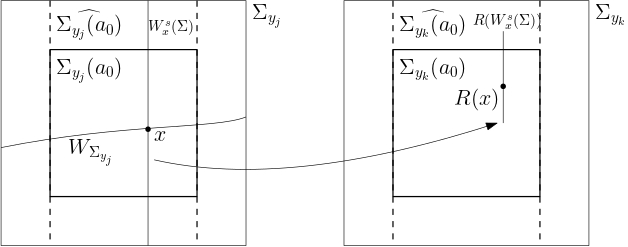
Figure 2. Sketch of cross-sections and sub-cross-sections together with the crossing $cu$-disk; and the definition of the Poincaré time at a given point in the $cu$-disk and the corresponding Poincaré map on the stable leaf.

For each equilibrium $\sigma\in\Lambda$, we let $V_{\sigma}$ be an open neighborhood of $\sigma$ on which the flow is linearizable. Let $\gamma^{s}_{\sigma}$ and $\gamma^{u}_{\sigma}$ denote the local stable and unstable manifolds of $\sigma$ within $V_{\sigma}$; trajectories starting in $V_{\sigma}$ remain in $V_{\sigma}$ for all future time if and only if they lie in $\gamma^{s}_{\sigma}$.

Define $V_{0}=\bigcup_{\sigma\in\operatorname{Sing}(G)\cap U}V_{\sigma}$. We shrink the neighborhoods $V_{\sigma}$ so that they are disjoint; $\Lambda\not\subset V_{0}$; and $\gamma^{u}_{\sigma}\cap\partial V_{\sigma}\subset\cup_{i=1}^{\ell_{\sigma}}V_{y_{i}}(a_{0})$ for some regular points $y_{i}=y_{i}(\sigma),i=1,\dots,\ell_{\sigma}$.

By compactness of $\Lambda$, there exists $\ell\in{\mathbb{Z}}^{+}$ and regular points $y_{1},\dots,y_{\ell}\in\Lambda$ such that $\Lambda\setminus V_{0}\subset\bigcup_{j=1}^{\ell}V_{y_{j}}(a_{0})$. We enlarge the set $\{y_{j}\}$ to include the points $y_{i}(\sigma)$ mentioned above; adjust the positions of the cross-sections $\Sigma_{y_{j}}$ if necessary to ensure that they are disjoint; and define the global cross-section $\Xi=\bigcup_{j=1}^{\ell}\Sigma_{y_{j}}$ and its smaller version $\Xi(a)=\bigcup_{j=1}^{\ell}\Sigma_{y_{j}}(a)$ for each $a\in(0,1)$. We also set $\widehat{\Xi(a)}=\bigcup_{j=1}^{\ell}\widehat{\Sigma_{y_{j}}(a)}$ for future reference.

In what follows we modify the choices of $U_{0}$ and $T_{0}$. However, $V_{y_{j}}$, $\Sigma_{y_{j}}$ and $\Xi$ remain unchanged from now on and correspond to our current choice of $U_{0}$ and $T_{0}$. All subsequent choices will be labeled $U_{1}\subset U_{0}$ and $T_{1}\geq T_{0}$. In particular $U_{1}\subset V_{0}\cup\bigcup_{j=1}^{\ell}V_{y_{j}}(a_{0})$. We set $\delta_{0}=d(\partial\Xi,\partial\Xi(a_{0}))>0$ where $\partial\Xi(a)$ is the boundary of the submanifold $\Xi(a)$ of $M$, $a\in(0,1)$, and $\Xi=\Xi(1)$.

For future use, for each $j=1,\dots,l$ we write $\Pi_{j}:\widehat{V_{y_{j}}(a)}\to\widehat{\Sigma_{y_{j}}(a)}$ for the projection along flow lines within the sub-flow box $\widehat{V_{y_{j}}(a)}$, that is, $x\in\widehat{V_{y_{j}}(a)}$ and $\Pi_{j}x\in\widehat{\Sigma_{y_{j}}(a)}$ belong to the same flow line within $\widehat{V_{y_{j}}(a)}$. We note that, since this a finite collection of smooth maps, there exists $L>0$ so that $\Pi_{j}$ is $L$-Lipschitz for all $j=1,\dots,l$.

3.4.2. The Poincaré map

By Theorem 3.3, for any $\delta>0$ we can choose $T_{1}\geq T_{0}$ such that $\operatorname{diam}\phi_{t}(W^{s}_{x}(\Sigma_{y_{j}}))<\delta$, for all $x\in\Sigma_{y_{j}}$, $j=1,\dots,\ell$ and $t>T_{1}$. We fix $T_{1}=T_{1}(\delta)$ for $L\cdot\delta=\delta_{0}=d(\partial\Xi,\partial\Xi(a_{0}))$ in what follows.

We define $\Gamma_{0}=\{x\in\Xi:\phi_{T_{1}+1}(x)\in\bigcup_{\sigma\in\operatorname{Sing}(G)\cap U_{0}}(\gamma^{s}_{\sigma}\setminus\{\sigma\})\}$ and $\Xi^{\prime}=\Xi\setminus\Gamma_{0}$. If $x\in\Xi^{\prime}$, then $\phi_{T_{1}+1}(x)$ cannot remain inside $V_{0}$ so there exists $t>T_{1}+1$ and $j=1,\dots,\ell$ such that $\phi_{t}x\in V_{y_{j}}(a_{0})$. Since $\varepsilon_{0}<1$, there exists $t>T_{1}$ such that $\phi_{t}x\in\Sigma_{y_{j}}(a_{0})$.

For each $\Sigma=\Sigma_{y_{j}}\in\Xi$, we choose a center-unstable disk $W_{\Sigma}$ which crosses $\Sigma$ and is transversal to ${\mathcal{W}}^{s}(\Sigma)$, that is, every stable leaf $W^{s}_{x}(\Sigma)$ intersects $W_{\Sigma}$ transversely at only one point, for each $x\in\Sigma$.

For every given fixed $x\in W_{\Sigma}\cap\Xi^{\prime}$, we define

$$R(x)=\phi_{\tau(x)}(x)\quad\text{where}\quad\tau(x)=\inf\left\{t>T_{1}:\phi_{t}x\in\bigcup_{j=1}^{\ell}\Sigma_{y_{j}}(a_{0})\right\}.$$

Thus, there exists $k\in\{1,\dots,\ell\}$ so that

$$\tau_{k}(x)=\inf\left\{t>T_{1}:\phi_{t}x\in\Sigma_{y_{k}}(a_{0})\right\}$$

equals $\tau(x)$. We note that by the choice of $T_{1}=T_{1}(\delta)$ we have $\operatorname{diam}\phi_{\tau(x)}(W^{s}_{x}(\Sigma))<\delta=\delta_{0}/L$ and so the disk $\phi_{\tau(x)}(W^{s}_{x}(\Sigma))$, although not necessarily contained in any $\widehat{\Sigma_{y_{j}}(a_{0})}$, is certainly contained in $\widehat{V_{y_{k}}(a_{0})}$ by construction and so $\Pi_{j}\big{(}\phi_{\tau(x)}(W^{s}_{x}(\Sigma))\big{)}\subset\widehat{\Sigma_{y_{k}}(a_{0})}$. Hence, we can define for each $y\in{\mathcal{W}}^{s}_{x}(\Sigma)$

$$R(y)=\phi_{\tau(y)}(y)\quad\text{where}\quad\tau(y)=\inf\left\{t>T_{1}:\phi_{t}y\in\widehat{\Sigma_{y_{k}}(a_{0})}\right\};$$ (3.1)

see Figure 2 for a sketch of this procedure. Note that since $\widehat{\Sigma_{y_{k}}(a_{0})}\supset\Sigma_{y_{k}}(a_{0})$, the above definitions of $\tau(x)$ and $\tau(y)$ coincide for $y=x$ and, by the Tubular Flow Theorem, the definition (3.1) provides a smooth extension of the previous definition for $x\in W_{\Sigma}\cap\Xi^{\prime}$ to the whole $W^{s}_{x}(\Sigma)$ and also to a neighborbood of $W^{s}_{x}(\Sigma)$ in $\Xi^{\prime}$.

Remark 3.6.

Let $C$ be the non-empty connected component of the set $\big{(}R\mid_{W_{\Sigma}}\big{)}^{-1}(\Sigma_{y_{k}}(a_{0}))$ of $W_{\Sigma}$ containing $x$. Then $R\mid_{W^{s}_{C}(\Sigma)}:W^{s}_{C}(\Sigma)\to\Sigma_{y_{k}}(a_{0})$ is smooth in the open sub-cross-section $W^{s}_{C}(\Sigma):=\cup\{W^{s}_{z}(\Sigma):z\in C\}\subset\Sigma$. In Figure 2, we sketch a situation where the connected component $C$ is strictly inside $W_{\Sigma}$.

Moreover, the union of the connected components of $\big{(}R\mid_{W_{\Sigma}}\big{)}^{-1}(\Sigma_{y_{k}}(a_{0})),k=1,\dots,\ell$ covers $W_{\Sigma}$ except for the subset of points sent to the boundary of $\Xi^{\prime}$.

We define the topological foliation ${\mathcal{W}}^{s}(\widehat{\Xi})=\bigcup_{j=1}^{\ell}{\mathcal{W}}^{s}(\widehat{\Sigma_{y_{j}}(a_{0})})$ of $\widehat{\Xi(a_{0})}$ with leaves $W^{s}_{x}(\widehat{\Xi})$ passing through each $x\in\widehat{\Xi(a_{0})}$. From the uniform contraction of stable leaves together with the choice of $T_{1}$, $\delta$ and $\delta_{0}$, we deduce that

$$\operatorname{diam}\left(\Pi\big{(}\phi_{\tau(x)}W^{s}_{x}(\widehat{\Xi})\big{)}\right)<L\delta=\delta_{0}$$

and then by the flow invariance of ${\mathcal{W}}^{s}$ and the previous definition of the Poincaré map $R$, we conclude that

$$R(W^{s}_{x}(\widehat{\Xi}))=\Pi\big{(}\phi_{\tau(x)}W^{s}_{x}(\widehat{\Xi})\big{)}\subset W^{s}_{Rx}(\widehat{\Xi}).$$

This proves the following

Proposition 3.7.

For big enough $T_{1}>T_{0}$, $R(W^{s}_{x}(\widehat{\Xi}))\subset W^{s}_{Rx}(\widehat{\Xi})$ for all $x\in\widehat{\Xi}^{\prime}=\widehat{\Xi(a_{0})}\setminus\Gamma_{0}$.

In this way we obtain a piecewise $C^{1}$ global Poincaré map $R:\widehat{\Xi}^{\prime}\to\widehat{\Xi(a_{0})}$ with piecewise $C^{1}$ roof function $\tau:\widehat{\Xi}^{\prime}\to[T_{1},\infty)$, and deduce the following standard result.

Lemma 3.8.

[7, Lemma 3.2] If the section $\widehat{\Sigma_{y}(a_{0})}$ contains no equilibria (i.e. $\Gamma_{0}\cap\widehat{\Sigma_{y}(a_{0})}=\emptyset$), then $\tau\mid_{\widehat{\Sigma_{y}(a_{0})}}\leq T_{1}+2$. In general, there is $C>0$ so that $\tau(x)\leq-C\log\operatorname{dist}(x,\Gamma_{0})$ for all $x\in\widehat{\Xi}^{\prime}$; moreover, $\tau(x)\nearrow\infty$ as $\operatorname{dist}(x,\Gamma_{0})\searrow 0$.

We define $\partial^{s}\widehat{\Xi(a_{0})}=\bigcup_{j=1}^{\ell}\partial^{s}\widehat{\Sigma_{y_{j}}(a_{0})}$ and $\Gamma_{1}=\{x\in\widehat{\Xi}^{\prime}:R(x)\in\partial^{s}\widehat{\Xi(a_{0})}\}$ and then set $\Gamma=\Gamma_{0}\cup\Gamma_{1}$. Clearly $\Gamma_{0}\cap\Gamma_{1}=\emptyset$.

Lemma 3.9.

1. $\Gamma_{0}$ is a $d_{s}$-submanifold of $\Xi$ given by a finite union of stable leaves $W_{s_{i}}(\Xi),i=1,\dots,k$; and

2. $\Gamma_{1}$ is a regular embedded $(d-2)$-topological submanifold foliated by stable leaves from ${\mathcal{W}}^{s}(\Xi)$ with finitely many connected components.

Remark 3.10.

Note that $\Gamma_{0}$ is a (smooth) submanifold of $\Xi$ with codimension $d_{cu}-1$, so it separates $\Xi$ only if $d_{cu}=2$; while $\Gamma_{1}$ is a regular topological codimension $1$ submanifold of $\Xi$ and so it separates $\Xi$.

Proof.

It is clear that $W^{s}_{x}(\Xi)\subset\Gamma$ for all $x\in\Gamma$, so $\Gamma$ is foliated by stable leaves. We claim that $\Gamma$ is precisely the set of those points of $\Xi$ which are sent to the boundary of $\Xi$ or never visit $\Xi$ in the future.

Indeed, if $x_{0}\in\widehat{\Xi}^{\prime}\setminus\Gamma_{1}$, then $R(x_{0})=\phi_{\tau(x_{0})}(x_{0})\in\Sigma^{\prime}$ for some $\Sigma^{\prime}\in\widehat{\Xi(a_{0})}=\{\widehat{\Sigma_{y_{j}}(a_{0})}\}$. For $x$ close to $x_{0}$, it follows from continuity of the flow that $R(x)\in\widetilde{\Sigma}^{\prime}$ (with $\tau(x)$ close to $\tau(x_{0})$). Hence $x\in\widehat{\Xi}^{\prime}\setminus\Gamma_{1}$ and since $\widehat{\Xi}^{\prime}=\widehat{\Xi}\setminus\Gamma_{0}$, then the claim is proved and, moreover, $\Gamma$ is closed.

For item (1), we note that $\Gamma_{0}\subset\Xi\cap\phi^{-1}_{[0,T_{1}+1]}\big{(}\bigcup_{\sigma}\gamma^{s}_{\sigma}\big{)}$ and we may assume without loss of generality that the above union comprises only generalized Lorenz-like equilibria; cf. Remark 3.2(2). Hence $T_{w}\gamma_{\sigma}^{s}=E^{cs}_{w}$ for $w\in\gamma_{\sigma}^{s}\setminus\{\sigma\}$; see Remark 3.2(1). Thus $\Gamma_{0}$ is contained in the transversal intersection between a compact $(d_{s}+1)$-submanifold and a compact $(m-1)$-manifold, so $\Gamma_{0}$ is a compact differentiable $d_{s}$-submanifold of $M$ and $\Xi$. In addition, since $\Gamma_{0}$ is foliated by stable leaves which are $d_{s}$-dimensional, then $\Gamma_{0}$ has only finitely many connected components in $\Xi$.

For item (2), note that for each $x\in\Gamma_{1}$ we have that $R(x)\in\partial\widehat{\Sigma_{j}(a_{0})}\subset\Sigma_{j}$. Thus there exists a neighborhood $W_{x}$ of $x$ in $\Xi$ and $V_{Rx}$ of $R(x)$ in $\Sigma_{j}$ so that $R\mid W_{x}:W_{x}\to V_{Rx}$ is a diffeomorphism. Hence $\Gamma_{1}\cap W_{x}=(R\mid W_{x})^{-1}(V_{x}\cap\partial^{s}\widehat{\Sigma(a_{0})})$ is homeomorphic to a $(d_{cu}-2+d_{s})$-dimensional disk. Moreover, this shows that the topology of $\Gamma_{1}$ is the same as the subspace topology induced by the topology of $\Xi$. We conclude that $\Gamma_{1}$ is a regular topological $(m-2)$-dimensional submanifold.

It remains to rule out the possibility of existence of infinitely many connected components $\Gamma_{1}^{k},k\in{\mathbb{Z}}^{+}$ of $\Gamma_{1}$ in $\Xi$. Since $\Xi$ contains finitely many sections only, then there exists cross-sections $\Sigma_{j},\Sigma_{i}$ in $\Xi$ and, taking a subsequence if necessary, an accumulation set $\widetilde{\Gamma}=\lim_{k}\Gamma_{1}^{k}$ within $\operatorname{Closure}(\Sigma_{j})$ so that $R(\Gamma_{1}^{k})\subset\partial^{s}\widehat{\Sigma_{i}(a_{0})}$ for all $k\geq 1$. By the continuity of the stable foliation, $\widetilde{\Gamma}$ is an union of stable leaves.

We claim that the Poincaré times $\tau(x_{k})$ for $x_{k}\in\Gamma_{1}^{k},k\geq 1$ are uniformly bounded from above. For otherwise the trajectory $\phi_{[0,\tau(x_{k})]}(x_{k})$ intersects $V_{\sigma}$ for some $\sigma\in\operatorname{Sing}(G)\cap U$ and accumulates $\sigma$. Hence, by the local behavior of trajectories near saddles and the choice of the cross-sections near $V_{\sigma}$, we get that $\widetilde{\Gamma}\subset\widetilde{\Sigma_{i}(a_{0})}$ is not contained in the boundary of the cross-section. This contradiction proves the claim. Let $T$ be an upper bound for $\tau(x_{k})$.

Then, for an accumulation point $x\in\widetilde{\Gamma}$ of $(x_{k})_{k\geq 1}$ we have that the trajectories $\phi_{[0,T]}(x_{k})$ converge in the $C^{1}$ topology (taking a subsequence if necessary) to a limit curve $\phi_{[0,T]}(x)$ and so $R(x)=\phi_{\tau(x)}(x)\in\partial^{s}\widehat{\Sigma_{i}(a_{0})}$. Thus we can find neighborhoods $W_{x}$ of $x$ and $V_{Rx}$ of $R(x)$ in $\Xi$ so that for arbitrarily large $m$ we have that $R\mid W_{x}:W_{x}\to V_{Rx}$ is a diffeomorphism and $\Gamma_{1}\cap W_{x}=(R\mid W_{x})^{-1}(V_{x}\cap\partial^{s}\widehat{\Sigma_{i}(a_{0})})$, which contradicts the regularity of $\Gamma_{1}$ as topological submanifold. This concludes the proof of item (2) and the lemma. ∎

From now on we set $\Xi^{\prime\prime}=\widehat{\Xi(a_{0})}\setminus\Gamma$. Then $\Xi^{\prime\prime}=S_{1}\cup\dots\cup S_{k}$ for some fixed $k\geq 1$, where each $S_{i}$ is a connected smooth strip, homeomorphic to either

• $\mathcal{D}^{d_{cu}}\times\mathcal{D}^{d_{s}}$, if $\Gamma_{0}\cap\operatorname{Closure}{S_{i}}=\emptyset$; or

• $\mathcal{D}^{d_{cu}}\times(\mathcal{D}^{d_{s}}\setminus\{0\})$, otherwise.

The latter are singular (smooth) strips.

We note that $R\mid S_{i}:S_{i}\to\widehat{\Xi(a_{0})}$ is a diffeomorphism onto its image, $\tau\mid S_{i}:S_{i}\to[T_{1},\infty)$ is smooth for each $i$, $\tau\mid S_{i}\leq T_{1}+2$ on non-singular strips $S_{i}$ and also on a neighborhood of $\partial^{s}(S_{i}\cup\Gamma_{0})$ for singular strips $S_{i}$. The foliation ${\mathcal{W}}^{s}(\Xi)$ restricts to a foliation ${\mathcal{W}}^{s}(S_{i})$ on each $S_{i}$.

Remark 3.11.

In what follows it may be necessary to increase $T_{1}$ leading to changes to $R$, $\tau$, $\Gamma$ and $\{S_{i}\}$ (and the constant $C$ in Lemma 3.8); see Remark 4.6. However, the global cross-sections $\Xi=\bigcup\Sigma_{y_{j}}$; $\Xi(a_{0})$ and $\widehat{\Xi(a_{0})}=\bigcup\widehat{\Sigma_{y_{j}}(a_{0})}$ are fixed throughout the argument.

Remark 3.12.

Since $R$ sends $\Xi^{\prime\prime}$ into the subsections $\widehat{\Xi(a_{0})}$ of $\Xi=\Xi(1)$, there are smooth extensions $\widetilde{R_{i}}:\widetilde{S_{i}}\to\Xi$ of $R\mid S_{i}:S_{i}\to\widehat{\Xi(a_{0})}$, where $\tilde{S}_{i}\supset\operatorname{Closure}(S_{i})\setminus\Gamma_{0}$.

3.5. Hyperbolicity of the global Poincaré map

We assume from now on that $\Lambda$ is a sectional hyperbolic attracting set with $d_{cu}\geq 2$ and proceed to show that, for large enough $T_{1}>1$, the global Poincaré map $R:\Xi^{\prime\prime}\to\Xi$ is piecewise uniformly hyperbolic (with discontinuities and singularities).

Let $S\in\{S_{i}\}$ be one of the smooth strips. Then there are cross-sections $\Sigma$, $\widetilde{\Sigma}\in\Xi$ so that $S\subset\Sigma$ and $R(\Sigma)\subset\widetilde{\Sigma}$. The splitting $T_{U}M=E^{s}\oplus E^{cu}$ induces the continuous splitting $T\Sigma=E^{s}(\Sigma)\oplus E^{u}(\Sigma)$, where $E^{s}_{x}(\Sigma)=(E^{s}_{x}\oplus{\mathbb{R}}\{G(x)\})\cap T_{x}{\Sigma}$ and $E^{u}_{x}(\Sigma)=E^{cu}_{x}\cap T_{x}{\Sigma}$ for $x\in\Sigma$; and analogous definitions apply to $\widetilde{\Sigma}$.

Proposition 3.13.

The splitting $T\Sigma=E^{s}(\Sigma)\oplus E^{u}(\Sigma)$ is

invariant:

$DR\cdot E^{s}_{x}(\Sigma)=E^{s}_{Rx}(\widetilde{\Sigma})$ for all $x\in S$, and $DR\cdot E^{u}_{x}(\Sigma)=E^{u}_{Rx}(\widetilde{\Sigma})$ for all $x\in\Lambda\cap S$.

uniformly hyperbolic:

for each given $\lambda_{1}\in(0,1)$ there exists $T_{1}>0$ so that if $\inf\tau>T_{1}$, then $\|DR\mid E^{s}_{x}(\Sigma)\|\leq\lambda_{1}$ and $\|\big{(}DR\mid E^{u}_{x}(\Sigma)\big{)}^{-1}\|\geq\lambda_{1}^{-1}$ for all $x\in S$ and $S\in\{S_{i}\}$.

Moreover, there exists $0<\widetilde{\lambda_{1}}<\lambda_{1}$ so that, for all $x$ on a non-singular strip $S$, or for $x$ on a neighborhood of $\partial^{s}(S\cup\Gamma_{0})$ of a singular strip $S$ we have $\widetilde{\lambda_{1}}<\|\big{(}DR\mid E^{s}_{x}(\Sigma)\big{)}^{-1}\|$ and $\|DR\mid E^{u}_{x}(\Sigma)\|<\widetilde{\lambda_{1}}^{-1}$.

Proof.

See [7, Proposition 4.1] with straightforward adaptation to use area expansion along each two-dimensional subspaces within $E^{u}_{x}(\Sigma)$ in order to obtain uniform expansion; cf. [8, Lemma 8.25]. The last statement follows from the boundedness of $\tau$ on the designated domains; cf. Lemma 3.8. ∎

For a given $a>0$, $x\in\Sigma$ and $\Sigma\in\Xi$ we define the unstable cone field at $x$ as $\mathcal{C}^{u}_{x}(\Sigma,a)=\{w=w^{s}+w^{u}\in E^{s}_{x}(\Sigma)\oplus E^{u}_{x}(\Sigma):\|w^{s}\|\leq a\|w^{u}\|\}.$

Proposition 3.14.

For any $a>0$, $\lambda_{1}\in(0,1)$, we can increase $T_{1}$ and shrink $U_{1}$ such that if $\inf\tau>T_{1}$ then $DR(x)\cdot\mathcal{C}^{u}_{x}(S,a)\subset\mathcal{C}^{u}_{Rx}(S^{\prime},a)$; and $\|DR(x)w\|\geq\|\pi^{u}DR(x)w\|\geq\lambda_{1}^{-1}\|w\|$ for all $w\in\mathcal{C}^{u}_{x}(S,a)$ and all $x\in S$ and $S,S^{\prime}\in\{S_{i}\}$ so that $fx\in S^{\prime}$. Moreover $\|DR(x)w\|\leq\widetilde{\lambda_{1}}^{-1}\|w\|$ for $x$ in a non-singular $S$ or $x$ in a neighborhood of $\partial^{s}(S\cup\Gamma_{0})$ for a singular $S$.

Proof.

See [7, Proposition 4.2], use $\widetilde{\lambda_{1}}$ from Proposition 3.13 and an uniform bound for $\|\pi^{u}\|$ depending on the angle between stable and center-unstable directions and the width of the cone. ∎

Considering the union of the smooth strips $S$, the previous results shows that we obtain a global continuous uniformly hyperbolic splitting $T\Xi^{\prime\prime}=E^{s}(\Xi)\oplus E^{u}(\Xi)$ in the following sense.

Theorem 3.15.

For given $a>0$ and $\lambda_{1}\in(0,1)$ we obtain a global Poincaré map $f$ so that the stable bundle $E^{s}(\Xi)$ and the restricted splitting $T_{\Lambda}\Xi^{\prime\prime}=E^{s}_{\Lambda}(\Xi)\oplus E^{u}_{\Lambda}(\Xi)$ are $DR$-invariant; and $DR\cdot\mathcal{C}^{u}_{x}(\Xi,a)\subset\mathcal{C}^{u}_{fx}(\Xi,a)$ and $\|\pi_{u}Df(x)w\|\geq\lambda_{1}^{-1}\|w\|$ for all $x\in\Xi^{\prime\prime}$ and $w\in\mathcal{C}^{u}_{x}(\Xi,a)$.

Remark 3.16.

The extensions $\widetilde{R_{i}}:\widetilde{S_{i}}\to\Xi$ mentioned in Remark 3.12 are such that on $\widetilde{S_{i}}\setminus\operatorname{Closure}S_{i}$ the map $\widetilde{R_{i}}$ behaves as $R$ in Propositions 3.13 and 3.14. In particular, $\delta_{1}=d(S_{i},\partial\widetilde{S_{i}})\geq\widetilde{\lambda_{1}}\cdot d(\Xi(a_{0}),\Xi)=\widetilde{\lambda_{1}}\delta_{0}$.

3.6. Distance between points on distinct stable leaves in cross-sections

Our argument to prove expansiveness hinges on showing that the distance between points on distinct stable leaves through points on close by orbits must increase at a definite rate. For that we relate distance between stable leaves on cross-sections with the distance between their images on the quotient map.

In the codimension-two case, that is, if $d_{cu}=2$, we use the one-dimensional central-unstable cone field restricted to the cross-sections to obtain the following.

Lemma 3.17.

Let us assume that $d_{cu}=2$ and that $a>0$ has been fixed, sufficiently small. Then there exists a constant $\kappa$ such that, for any pair of points $x,y\in\Sigma\in\Xi$, and any $cu$-curve $\gamma:[0,1]\to\Sigma$ joining $x$ to some point of $W^{s}(y,\Sigma)$, we have $\ell(\gamma)\leq\kappa\cdot d(x,y)$, where $\ell(\gamma)=\int_{0}^{1}\|\dot{\gamma}\|$ is the length of $\gamma$ in the induced distance Riemannian distance on $\Sigma$.

Proof.

This is basically [8, Lemma 6.18] from the singular-hyperbolic setting conveniently restated in the codimension-two setting. ∎

For this result it is crucial that the center-unstable cones $C^{cu}_{x}(\Sigma,a)$ on cross-sections $\Sigma\in\Xi$ have one-dimensional core, that is, they are cones around a certain one-dimensional subspace of the tangent space $T_{x}\Sigma$; see the left hand side of Figure 3.

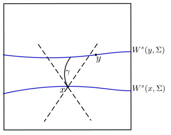
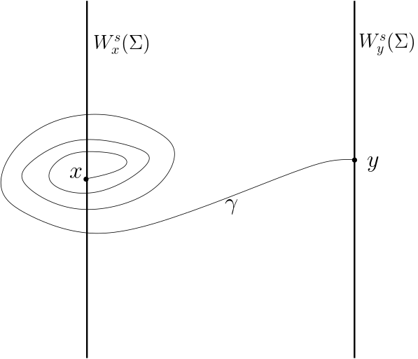
Figure 3. A sketch of a $cu$-curve connecting two stable leaves on a cross-section with $d_{cu}=2$, on the left; and a possible $cu$-curve connecting two stable leaves on a higher codimensional setting, on the right.

3.6.1. Construction of a $C^{1}$ local chart

For higher codimensions $d_{cu}>2$ there exist $cu$-curves connecting two stable leaves which behave like tightly curved helixes, loosing any relation between the lenght of a general $cu$-curve and the distance between the leaves; see the right hand side of Figure 3. That is why we assume the extra hypotheses of $1$-strong-dissipativeness in the higher codimensional setting.

We have seen the topological foliation $\mathcal{W}^{s}$ of $U_{0}$ induces a topological foliation $\mathcal{W}^{s}(\Sigma)=\{W^{s}_{x}(\Sigma)\}_{x\in\Sigma}$ on each $\Sigma$. For a $1$-strongly dissipative $C^{1}$ vector field $G$, Theorem 3.4 guarantees that the foliation $\mathcal{W}^{s}$ is $C^{1}$, that is, the map

$$\gamma:U_{0}\to\textrm{Emb}^{1}(\mathcal{D}^{d_{s}},\Sigma),\quad\text{such that}\quad\gamma(x)(0)=x\text{ and }\gamma(x)(\mathcal{D}^{d_{s}})=W^{s}_{x}$$

in the notation of Theorem 3.3 satisfies that $(x,y)\in U_{0}\times\mathcal{D}^{d_{s}}\mapsto\gamma(x)(y)$ becomes a local $C^{1}$ diffeomorphism.

Considering the transversal disk $W_{\Sigma}$ in $\Sigma$, we have that $W_{\Sigma}$ is diffeomorphic to $\mathcal{D}^{d_{cu}-1}$ and define the local chart $\psi:\mathcal{D}^{d_{cu}-1}\times\mathcal{D}^{d_{s}}\to\Sigma$ by $\psi(x,y)=\gamma(x)(y)$. Thus $\psi(\{x\}\times\mathcal{D}^{d_{s}})=\gamma_{x}(\mathcal{D}^{d_{s}})=W^{s}(x,\Sigma)$ and $\psi$ is a $C^{1}$ chart of $\Sigma$.

Lemma 3.18.

There are constants $K,L>0$ such that

$$L\cdot d_{e}(x,y)\leq d(W^{s}_{x}(\Sigma),W^{s}_{y}(\Sigma))\leq K\cdot d_{e}(x,y),$$

where $d$ and $d_{e}$ denote the Riemannian distance and the Euclidean distance, respectively.

Proof.

By definition $d(W^{s}_{x}(\Sigma),W^{s}_{y}(\Sigma))=\inf_{\xi}\ell(\xi)$, where $\ell(\xi)$ is the length of the curve $\xi$ connecting some point of $W^{s}_{x}(\Sigma)$ to another point of $W^{s}_{y}(\Sigma)$ inside $\Sigma$. Since $\psi$ is a diffeomorphism, $\xi$ is the image of some curve $\tilde{\xi}\in\mathcal{D}^{d_{cu}}\times\mathcal{D}^{d_{s}}$ connecting $\{x\}\times\mathcal{D}^{d_{s}}$ to $\{y\}\times\mathcal{D}^{d_{s}}$ and $\ell(\xi)=\int_{a}^{b}\|D\psi(\tilde{\xi})\cdot\tilde{\xi}^{\prime}(t)\|dt$. Then $\ell(\xi)\leq K\cdot\ell(\tilde{\xi})$ where $K=\sup_{x\in\Sigma}\|D\psi(x)\|$. Hence

$$d\big{(}W^{s}(x,\Sigma),W^{s}(y,\Sigma)\big{)} =\inf_{\xi}\ell(\xi)\leq K\inf_{\xi}\ell(\tilde{\xi})=K\cdot d_{e}(\{x\}\times\mathcal{D}^{d_{s}},\{y\}\times\mathcal{D}^{d_{s}})=K\cdot d_{e}(x,y).$$

Analogously, $\ell(\xi)\geq L\cdot\ell(\tilde{\xi})$ with $L=\inf_{x\in\Sigma}\|D\psi^{-1}(x)\|^{-1}$ and so

$$d\big{(}W^{s}(x,\Sigma),W^{s}(y,\Sigma)\big{)} =\inf_{\xi}\ell(\xi)\geq L\inf_{\xi}\ell(\tilde{\xi})=L\cdot d_{e}(\{x\}\times\mathcal{D}^{d_{s}},\{y\}\times\mathcal{D}^{d_{s}})=L\cdot d_{e}(x,y)$$

finishing the proof. ∎

3.7. The Poincaré quotient map on a cross-section

Recall the choice of a a center-unstable disk $W_{\Sigma}$ transversal to ${\mathcal{W}}^{s}(\Sigma)$ for each $\Sigma\in\widehat{\Xi(a_{0})}$, and consider the projection $\pi:\Sigma\to W_{\Sigma}$ in each $\Sigma\in\widehat{\Xi(a_{0})}$ which maps every $x\in\Sigma$ to the point $\pi(x)$ such that

$$W^{s}_{x}(\Sigma)\cap W_{\Sigma}=\{\pi(x)\}.$$

The quotiented cross-section is homeomorphic to $W_{\Sigma}$. Since the foliation ${\mathcal{W}}^{s}(\Sigma)$ is preserved by $R$, that is, $R({\mathcal{W}}^{s}_{x}(\Sigma))\subset{\mathcal{W}}^{s}_{Rx}(\Sigma^{\prime})$, where $R(x)\in\Sigma^{\prime}$, the Poincaré quotient map $f:{\mathcal{W}}_{\Sigma}\to{\mathcal{W}}_{\Sigma^{\prime}}$ is given by $f\circ\pi(x)=\pi\circ R(x)$.

3.7.1. The quotient map is expanding on the smooth strip

In the $d_{cu}>2$ case, since the vector field is assumed to be $1$-strongly dissipative, then we can use the $C^{1}$ local chart $\psi$.

We have that $\Sigma\cong\mathcal{D}^{d_{cu}-1}\times\mathcal{D}^{d_{s}}$, the stable foliation is given by $\big{\{}\{a\}\times\mathcal{D}^{d_{s}}\big{\}}$ and $W_{\Sigma}\cong\mathcal{D}^{d_{cu}-1}$. Then, in these coordinates, $\pi$ is given by the canonical projection on ${\mathbb{R}}^{d_{cu}-1}$, $\pi:\mathcal{D}^{d_{cu}-1}\times\mathcal{D}^{d_{s}}\to\mathcal{D}^{d_{cu}-1}$ and $f:\mathcal{D}^{d_{cu}-1}\to\mathcal{D}^{d_{cu}-1}$ can be written $f=\pi\circ R|_{\mathcal{D}^{d_{cu}-1}}$. In this setting the map $f$ is a piecewise $C^{1}$ map with smooth domains on each projected strip $\pi(S_{i})$.

Lemma 3.19.

Denote by $\pi(S_{i})$ a smooth strip of $f$ corresponding to the strip $S_{i}$ of $R$. There exists $\mu>1$ such that $\|Df(x)^{-1}\|\leq\mu^{-1}<1$, for every $x\in\pi(S_{i})$.

Proof.

Given a vector $v\in{\mathbb{R}}^{d_{cu}-1}$, there exists a curve $\gamma:I\to\mathcal{D}^{d_{cu}-1}$ with $\gamma(0)=x$ and $\gamma^{\prime}(0)=v$. This $\gamma$ is a $cu$-curve by construction and

$$Df(x)v=D(\pi\circ R)(x)(v)=D\pi(R(x))DR(x)v=\pi(R(x))DR(x)v.$$

Using the Proposition 3.14, we have: $\|Df(x)v\|=\|\pi(R(x))DR(x)v\|\geq\lambda_{1}^{-1}\|v\|.$ Hence, denoting $\mu=\lambda_{1}^{-1}$ we get $\|Df(x)^{-1}\|\leq\mu^{-1}$. ∎

Remark 3.20.

We also define extensions $\widetilde{f_{i}}:\pi(\widetilde{S_{i}})\to\Xi$ of $f\mid\pi(S_{i})$ satisfying $\widetilde{f_{i}}\circ\pi=\pi\circ\widetilde{R_{i}}$ which clearly have the same properties stated in Lemma 3.19.

4. Proof of robust expansiveness

Here we prove the main Theorems A and B.

Arguing by contradiction, we assume that the flow is not expansive on $U_{0}$, the trapping region containing $\Lambda$, that is, there exists $\varepsilon>0$ such that for all $\delta>0$, we can find $x,y\in U_{0}$ and $h\in S({\mathbb{R}})$ satisfying $\operatorname{dist}(\phi_{t}(x),\phi_{h(t)}(y))\leq\delta$ and $\phi_{h(t)}(y)\notin\phi_{[t-\varepsilon,t+\varepsilon]}(x)$ for all $t\in{\mathbb{R}}$. Then, we can take $\delta_{n}\searrow 0$, $x_{n},y_{n}\in U_{0}$ and $h_{n}\in S({\mathbb{R}})$ such that for all $t\in{\mathbb{R}}$

$$d(\phi_{t}(x_{n}),\phi_{h_{n}(t)}(y_{n}))\leq\delta_{n}\quad\text{and}\quad\phi_{h_{n}(t)}(y_{n})\notin\phi_{[t-\varepsilon,t+\varepsilon]}(x_{n}).$$ (4.1)

Since the set of accumulation points is not empty, there exists some regular point $z\in\Lambda$ which is accumulated by the sequence of $\omega$-limit sets $\omega(x_{n})$ in the following sense: there exists $z_{n}\in\omega(x_{n})$ for each $n\geq 1$ such that $z_{n}\to z$.

Using that ${\mathcal{C}}$ is a cover of $\Lambda$ and $\omega(x)\subset\Lambda$, we can assume without loss of generality that $z$ is inside some $\Sigma^{\delta}\in\Xi^{\delta}$. This guarantees that $d(z,\partial^{s}\Sigma)>\delta$. We can now choose a neighborhood $V$ of $z$ contained in $\Sigma^{\delta}(\varepsilon_{0})$ for which there exists $n_{0}>1$ such that $z_{n}\in V$ for all $n\geq n_{0}$.

Then, the orbit of $x_{n}$ returns infinitely often to a neighborhood of $z_{n}$ which, on its turn, is close to $z$ and inside $V$. For this, we can take $\delta_{n}$ small enough (if necessary) so that the orbit of $y_{n}$ visits $V$ infinitely many times.

Let $t_{n}$ be the corresponding time to the first intersection between the orbit of $x_{n}$ and $\Sigma^{\delta}$. Replacing $x_{n}$,$y_{n}$, $t$ and $h_{n}$ by $x^{(n)}=\phi_{t_{n}}(x_{n})$, $y^{(n)}=\phi_{h_{n}(t_{n})}(y_{n})$, $\tilde{t}=t-t_{n}$ and $\tilde{h}_{n}(\tilde{t})={h}_{n}(\tilde{t}+t_{n})-h_{n}(t_{n})$ we still have

$$d(\phi_{\tilde{t}}(x^{(n)}),\phi_{\tilde{h}_{n}(\tilde{t})}(y^{(n)}))\leq\delta_{n}\quad\text{and}\quad\phi_{{\tilde{h}}_{n}(\tilde{t})}(y^{(n)})\notin\phi_{[\tilde{t}-\varepsilon,\tilde{t}+\varepsilon]}(x^{(n)}).$$

Moreover, by construction of $V$, we can prove the following.

Proposition 4.1.

There exists $K>0$, depending only on the angle between $\Sigma$ and the direction of the flow (see figure 4), such that for every $n\geq 0$ there are sequences $(\tau_{n,j})$ (with $\tau_{n,0}=0$) and $(\upsilon_{n,j})$ such that

• $x_{n,j}=\phi_{\tau_{n,j}}(x^{(n)})\in\Sigma^{\delta}$ and $y_{n,j}=\phi_{\upsilon_{n,j}}(y)\in\Sigma^{\delta}$ for all $j\geq 0$, where $\upsilon_{n,j}=h(\tau_{n,j})+\varepsilon_{n,j}$;

• $\tau_{n,j}-\tau_{n,j-1}>T_{1}$;  $|\upsilon_{n,j}-h(\tau_{n,j})|<K\delta_{n}$ and $d(x_{n,j},y_{n,j})<K\delta_{n}$.

Proof.

This is contained in [9, Theorem 7.13]. The proof does not use (co)dimension nor hyperbolicity assumptions. ∎

We will fix a convenient $n$ in what follows and write $x=x^{(n)}$ and $y=y^{(n)}$. We observe that $\phi_{t}(x)$ and $\phi_{s}(y)$ are not in the local stable manifold $W^{s}_{loc}(\sigma)$ of some $\sigma\in Sing(\Lambda)$, for all $t,s\in{\mathbb{R}}$. For otherwise, these points could not return to $\Xi$ infinitely often. Then $R^{j}(x)$ and $R^{j}(y)$ are well-defined for all $j\geq 0$ and we write $x_{j}=R^{j}(x)$ and $y_{j}=R^{j}(y)$ in what follows.

Figure 4. The neighborhood $V$.

Remark 4.2.

Whenever $R(x_{j})=\phi_{\tau(x_{j})}(x_{j})$ and $R(y_{j})=\phi_{\tau(y_{j})}(y_{j})$ are in the same $\Sigma\in\Xi$, we can estimate as in Proposition 4.1 to ensure that $\tau(y_{j})=\tau(x_{j})+\varepsilon_{j}$ and so $d(R(x_{j}),R(y_{j}))<K(\Sigma)\delta_{n}$.

In general, we have that $x_{j+1}=R^{j}(x)\in\Xi(a)$ and we can find $\widetilde{\tau_{j+1}(y)}$ such that setting $\widetilde{y_{j+1}}=\widetilde{R}(y_{j})=\phi_{\widetilde{\tau_{j+1}(y)}}(y)\in\Sigma\in\Xi$ we get $x_{j+1}=R(x_{j})=\widetilde{R}(x_{j})\in\Sigma(a)$; and also $\widetilde{\tau(y)}=\tau(x_{j})+\varepsilon_{j}$.

Since there exists finitely many sections in $\Xi$, we can take an uniform constant $K$ such that $d(\widetilde{R}(x_{j}),\widetilde{R}(y_{j}))<K\delta_{n}$ for all $\Sigma\in\Xi$ such that $R(x_{j})$,$R(y_{j})\in\Sigma$.

Then $x_{j}=R^{j}(x)=\phi_{\tau(x_{j})}(x)$ is well-defined for all $j\geq 0$ and we set $y_{j}=\widetilde{R}(y_{j-1})=\phi_{\tau(y_{j})}(y)$ for all $j\geq 1$ in what follows.

The essential part of the proof of the main theorems is to deduce the following.

Theorem 4.3.

Given $\varepsilon_{0}>0$ there exists $\delta_{0}>0$ such that, if $x,y\in\Xi$ satisfy

1. there exist $\tau_{j}$ such that $x_{j}=\phi_{\tau_{j}}(x)\in\Xi$ with $\tau_{j}-\tau_{j-1}>T_{1}$ for all $j\geq 1$;

2. $d\big{(}\phi_{t}x,\phi_{h(t)}y\big{)}<\delta_{0}$ for all $t>0$ and some $h\in S({\mathbb{R}})$;

then there exists $j\geq 1$ and $\eta\in[\tau_{j}-\varepsilon_{0},\tau_{j}+\varepsilon_{0}]$ such that $\phi_{h(\tau_{j})}y\in{\mathcal{W}}^{s}_{\phi_{\eta}x}$.

We postpone the proof of this result to Subsection 4.2 and deduce now the statements of the main theorems.

4.1. Proof of the main Theorems A and B

We assume the conclusion of Theorem 4.3 and finish the proof of both main Theorems A and B, proceeding as in [9, Subsection 3.3.4].

We note the following geometric consequence of transversality of the flow to the stable foliation in $U_{0}$.

Lemma 4.4.

There exist small $\rho,c>0$, depending only on the flow, such that if $z_{1},z_{2},z_{3}$ are points in $U_{0}$ satisfying $z_{3}\in\phi_{[-\rho,\rho]}(z_{2})$ and $z_{2}\in B(z_{1},\rho)\cap{\mathcal{W}}_{z_{1}}^{s}$, with $z_{1}$ away from any equilibria, then $d(z_{1},z_{3})\geq c\cdot\max\{d(z_{1},z_{2}),d(z_{2},z_{3})\}.$

Proof.

This is a direct consequence of the fact that the angle between $E_{x}^{s}$ and the flow direction $G(x)$ is bounded from zero which, in its turn, follows from the fact that the latter is contained in the center-unstable sub-bundle $E^{cu}$; see e.g. [9, Lemma 3.2] or [8, Lemma 7.12] and the left hand side of Figure 5. ∎

Remark 4.5.

Since we may shrink the value of $c>0$ in Lemma 4.4, we assume without loss of generality that $10c<\sup\{\|G(z)\|:z\in\Xi\}$.

We fix $\varepsilon_{0}=\varepsilon$ as in (4.1) and then consider $\delta_{0}$ as given by Theorem 4.3.

Remark 4.6.

1. We fix $T_{1}$ large enough so that the construction of the global Poincaré return map, described in Section 3, provides $\lambda_{1}\in(0,1)$ satisfying $\mu^{-1}=\lambda_{1}<\min\{1/2,\kappa,L/K\}$, where the constants are given by Lemmas 3.18 and 3.19. From now on we fix $\Xi$ and the smooth strips $\{S_{i}\}\subset\Xi$.

2. We fix $n$ such that $\delta_{n}$ is sufficiently small according to the following conditions.

   • $\delta_{n}<\delta_{0}$ and $\delta_{n}<c^{2}\cdot\rho<c\rho$.

   • Suppose that $x_{j}$ and $y_{j}$ are in the same strip $S_{i}$ of $R$ and consequently $\hat{x_{j}}=\pi(x_{j})$ and $\hat{y_{j}}=\pi(y_{j})$ are in the same smooth domain of $\hat{S_{i}}=\pi(S_{i})$ of $f$. We can choose $\delta_{n}$ small enough so that, if the ball $B(x_{j},K\delta_{n})$ is not entirely contained in $S_{i}$, then $B(x_{j},K\delta_{n})$ shall be entirely contained in the smooth strip $\widetilde{S_{i}}$ of $\widetilde{R}$, the extension map of $R$; and $B(\hat{x_{j}},K\delta_{n})$ is contained in $\pi(\widetilde{S_{i}})$ the extended smooth domain of $\widetilde{f}$.

   • If $x_{j}$ and $y_{j}$ are not in the same smooth strip of $\Sigma$, then we can assume that $x_{j}$ and $y_{j}$ are in adjoining strips. Indeed, it is enough to take

     $$2K\delta_{n}<\min\{d(S_{j},S_{k}):S_{j},S_{k}\text{ are non-adjoining strips in }\Xi\}.$$

     Consequently, $y_{j}$ belongs to the extended domain $\widetilde{S}$ which contains $x_{j}$.

Now we apply Theorem 4.3 to $x=x_{0}=x^{(n)}$, $y=y_{0}=y^{(n)}$, $x_{j}=R^{j}(x_{0})=\phi_{\tau_{j}}(x_{0})$ and $h=h_{n}$: where hypothesis (1) corresponds to the choice of $\tau_{n,j}$ from Proposition 4.1 and, with these choices, hypothesis (2) follows by the choice of $x,y$ from (4.1).

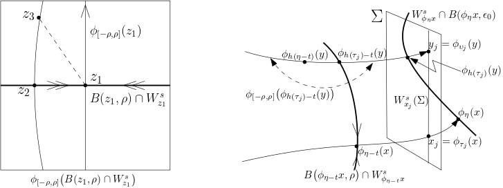
Figure 5. Sketch of the setting of Lemma 4.4 on the left; and of the proof of Theorems A and B using Theorem 4.3 on the right hand side.

Therefore, we obtain $\phi_{h(\tau_{j})}y\in B(\phi_{\eta}x,\varepsilon_{0})\cap{\mathcal{W}}^{s}(\phi_{\eta}x)$ for some $\eta\in[\tau_{j}-\varepsilon_{0},\tau_{j}+\varepsilon_{0}]$ and $j\geq 1$. From the right hand side of (4.1) we have $\phi_{h(\tau_{j})}y\neq\phi_{\eta}x$. Hence, since the leaves of the stable foliation are expanded under backward iteration, there exists a maximum $\theta>0$ such that for all $0\leq t\leq\theta$ (see the right hand side of Figure 5)

$$\phi_{h(\tau_{j})-t}y\in B(\phi_{\eta-t}x,\rho)\cap{\mathcal{W}}^{s}_{\phi_{\eta-t}x}\quad\text{and}\quad\phi_{h(\eta-t)}y\in\phi_{[-\rho,\rho]}(\phi_{h(\tau_{j})-t}y).$$

Moreover, $x_{j}$ is close to $\Xi$ which is uniformly bounded away from the equilibria, and then $\|G(\phi_{t}x_{j})\|\geq c$ for $0\leq t\leq\theta$. Since $\theta$ is maximum

$$\text{either }d\big{(}\phi_{h(\tau_{j})-t}y,\phi_{\eta-t}x\big{)} \geq\rho\text{ or }d\big{(}\phi_{h(\eta-t)}y,\phi_{h(\tau_{j})-t}y\big{)}\geq c\rho\text{ for }t=\theta.$$

Applying now Lemma 4.4 we deduce that $d\big{(}\phi_{\eta-t}x,\phi_{h(\eta-t)}y\big{)}\geq c^{2}\rho>\delta_{n}$ contradicting the choice of $x,y$ from (4.1). This completes the proof of expansiveness for $\phi_{t}$ in the trapping region $U_{0}$ of $\Lambda$ assuming Theorem 4.3.

4.1.1. On robustness of expansiveness

To obtain robustness of expansiveness, we observe that

1. there exists a neighborbood $\mathcal{V}\subset\mathcal{X}^{1}(M)$ of $G$ in the family of all $C^{1}$ vector fields with the $C^{1}$ topology for which the family $\Xi$ of adapted cross-sections for $\Lambda$ and $G$ remains a family of adapted cross-sections for $\Lambda_{Y}(U_{0})=\cap_{t>0}\overline{\psi_{t}U_{0}}$ and all $Y\in\mathcal{V}$, where $\psi_{t}$ is the flow generated by $Y$.

   This is a consequence of $C^{1}$ closeness between $Y$ and $G$ and the continuity of the map $Y\in\mathcal{V}\mapsto\Lambda_{Y}(U_{0})$ in the Hausdorff topology; this holds for every isolated set: see e.g. [8, Lemma 2.3].

2. Consequently, the hyperbolicity constants for the global Poincaré return map $R_{Y}$ can be taken uniform on $Y\in\mathcal{V}$, including the threshold time $T_{1}$ and the value of $K$.

3. Moreover, the smooth strips of $R_{Y}$ are uniformly close in the Riemannian distance to the corresponding strips of $R=R_{G}$, and so $\varepsilon_{0}$ and $\delta_{0}=\delta_{n}$ is the previous argument can also be taken uniformly on $Y\in\mathcal{V}$.

Hence, Theorem 4.3 holds for all $Y\in\mathcal{V}$ with constant values of $\varepsilon_{0}$ and $\delta_{0}$. This is enough to conclude that expansiveness is robust for all sectional-hyperbolic attracting sets in the setting of Theorems A and B.

This completes the proof of Theorems A and B assuming Theorem 4.3.

4.2. Proof of positive expansiveness

Now we prove Theorem 4.3. We first assume the following.

Claim 4.7.

For some $j\geq 0$ we have $x_{j}\in{\mathcal{W}}^{s}_{y_{j}}(\Xi)$.

By the invariance and uniqueness of the stable foliation (given by Theorem 3.3), this implies that $x_{j}\in{\mathcal{W}}^{s}_{y_{j}}(\Xi)$ and $y_{j}\in{\mathcal{W}}^{s}_{x_{j}}(\Xi)$ for all $j\geq 0$.

We postpone the proof of this claim and explain first, following [8, Section 7.2.7] and [9, Section 3.3.4], how Theorem 4.3 follows from Claim 4.7.

Proof of Theorem 4.3.

Let $j\geq 0$ be such that $y_{j}\in W^{s}(x_{j},\Sigma)$. Then, according to Proposition 4.1 and Remark 4.2, we have $|\tau(y_{j})-h(\tau(y_{j}))|=\varepsilon_{j}<K\cdot\delta_{0}$ and, by construction of the stable foliation on cross-sections, there exists a small $\bar{\varepsilon}>0$ such that $\phi_{t}(y_{j})\in{\mathcal{W}}^{s}_{x_{j}}$ for some $|t|<\bar{\varepsilon}$. Therefore the trajectory $\mathcal{O}_{y}=\phi_{[\tau(y_{j})-K\cdot\delta_{0}-\bar{\varepsilon},\tau(y_{j})+K\cdot\delta_{0}+\bar{\varepsilon}]}(y)$ must contain $\phi_{h(\tau(y_{j}))}(y)$. We note that this holds for all sufficiently small values of $\delta_{0}>0$ fixed from the beginning.

Let $\varepsilon_{0}>0$ be given and let us consider the piece of the orbit $\mathcal{O}_{x}:=\phi_{[\tau_{j}-\varepsilon_{0},\tau_{j}+\varepsilon_{0}]}(x)$ and the piece of the orbit of $x$ whose stable manifolds intersect $\mathcal{O}_{y}$, i.e.,

$${\mathcal{O}}_{xy}=\left\{\phi_{s}(x):\exists t\in[\tau(y_{j})-K\cdot\delta_{0}-\bar{\varepsilon},\tau(y_{j})+K\cdot\delta_{0}+\bar{\varepsilon}]\mbox{ s.t. }\phi_{t}(y)\in{\mathcal{W}}^{s}_{\phi_{s}(x)}\right\}.$$

Since $\phi_{t}(y_{j})\in{\mathcal{W}}^{s}_{x_{j}}$ we conclude that $\mathcal{O}_{xy}$ is a neighborhood of $x_{j}=\phi_{\tau_{j}}(x)$. Moreover, this neighborhood can be made as small as needed by letting $\delta_{0}$ and so $\bar{\varepsilon}$ small enough. In particular this ensures that $\mathcal{O}_{xy}\subset\mathcal{O}_{x}$ and so $\phi_{h(\tau_{j})}(y)\in\cup_{z\in\mathcal{O}_{x}}{\mathcal{W}}^{s}_{z}$. As this finishes the proof of Theorem 4.3 assuming Claim 4.7. ∎

4.3. Proof of the claim

We argue by contradiction, assumming that $y_{j}\notin W^{s}_{x_{j}}(\Xi)$ for all $j\geq 1$ and split the argument into the codimension two case and the higher codimension case. The goal is to show that the pairs $x_{j}$ and $y_{j}$ are either in the same smooth strip of the global Poincaré return map $R$, or else they are in the same extended smooth strip of the extension of the global Poincaré map $\widetilde{R}$.

4.3.1. The codimension-two case

Let us assume first that $x_{j}$ and $y_{j}$ are in the same strip $S_{i}$ of $R$ in some cross-section $\Sigma$ for some $j\geq 1$.

We can consider a $cu$-curve $\gamma:[0,1]\to S$ such that $\gamma(0)=x_{j}$ and $\gamma(1)\in{\mathcal{W}}^{s}_{y_{j}}(\Sigma)$ and

• by Proposition 3.7, we have invariance of the stable foliation inside cross-sections;

• by Proposition 3.13, we have invariance and expansion of $cu$-cones under iteration of smooth domains.

Hence $\zeta=R\circ\gamma$ is another $cu$-curve contained in some $\Sigma^{\prime}\in\Xi$ such that $\zeta(0)=x_{j+1}\in\Sigma^{\prime}$ and $\zeta(1)\in{\mathcal{W}}^{s}_{y_{j+1}}(\Sigma^{\prime})$ and, moreover, $\ell(\zeta)\geq\lambda_{1}^{-1}\ell(\gamma)$. Since we can find a point $\widehat{y_{j+1}}\in{\mathcal{W}}^{s}_{y_{j+1}}(\Xi)={\mathcal{W}}^{s}_{y_{j+1}}(\Sigma^{\prime})$ so that $d\big{(}x_{j+1},{\mathcal{W}}^{s}_{y_{j+1}}(\Xi)\big{)}=d\big{(}x_{j+1},\widehat{y_{j+1}}\big{)}$, we use the estimate of Lemma 3.17 to arrive at

$$d\big{(}x_{j+1},\widehat{y_{j+1}}\big{)}\geq\kappa\cdot\ell(\zeta)\geq\frac{\kappa}{\lambda_{1}}\ell(\gamma)\geq\frac{\kappa}{\lambda_{1}}\cdot d\big{(}x_{j},{\mathcal{W}}^{s}_{y_{j}}(\Xi)\big{)}$$

and so, see Figure 6

$$d\big{(}x_{j+1},{\mathcal{W}}^{s}_{y_{j+1}}(\Xi)\big{)}\geq 2\cdot d\big{(}x_{j},{\mathcal{W}}^{s}_{y_{j}}(\Xi)\big{)}.$$ (4.2)

Otherwise, if $x_{j},y_{j}$ are not in the same smooth strip, then they belong to adjoining smooth strips $S,S^{\prime}$ of $R$, by the choices made according to Remark 4.6, and $y_{j}$ belongs to $B(x_{j},K\delta_{n})=B(x_{j},K\delta_{0})$ contained in the extended strip $\widetilde{S}$ which is a smooth domain for $\widetilde{R}$. This prevents in particular that the boundary between $S$ and $S^{\prime}$ is a singular line, since then $y_{j+1}$ and $x_{j+1}$ would be in distinct cross-sections, which is impossible.

Figure 6. Expansion of distance between stable leaves.

We may now repeat the previous argument using the uniform expansion of central-unstable curves to again conclude (4.2). Therefore, in both cases, we conclude by induction on $j\geq 1$ that

$$d\big{(}x_{j},{\mathcal{W}}^{s}_{y_{j}}(\Xi)\big{)}\geq 2^{j}\cdot d\big{(}x_{0},{\mathcal{W}}^{s}_{y_{0}}(\Xi)),\quad j\geq 1.$$

However, we have by assumption that $d\big{(}x_{0},{\mathcal{W}}^{s}_{y_{0}}(\Xi))>0$ and

$$d\big{(}x_{j},{\mathcal{W}}^{s}_{y_{j}}(\Xi)\big{)}\leq d(x_{j},y_{j})\leq\delta_{0},\quad j\geq 0.$$

This yields a contradiction which proves that $x_{j}\in{\mathcal{W}}^{s}_{y_{j}}(\Xi)$ for some (and then, all) $j\geq 0$.

4.3.2. The higher codimensional case

In the $d_{cu}>2$ case, let us assume again that $x_{j}$ and $y_{j}$ are in the same strip $S_{i}$ of $R$ in some cross-section $\Sigma$. Then $\widehat{x_{j}}=\pi(x_{j})$ and $\hat{y_{j}}=\pi(y_{j})$ are in the smooth domain $\widehat{S_{i}}=\pi(S_{i})$ of $f$. Let $S_{j}$ be the smooth domain where $x_{j+1}$ lies and $\widehat{S_{j}}=\pi(S_{j})$ the corresponding domain of $f$.

By the choices of constants according to Remark 4.6, we get that $B=B(\widehat{x_{j+1}},K\delta_{n})$ is contained in the extended strip $\widetilde{S_{j}}=\pi(\bar{S_{j}})$ and $B$ contains then line segment $[\widehat{x_{j+1}},\widehat{y_{j+1}}]$.

Since $\widehat{x_{j+1}}=f(\widehat{x_{j}})$ and $\widehat{y_{j+1}}=f(\widehat{y_{j}})\in B$, we can apply the Mean Value Theorem to $g=\big{(}f\mid_{B}\big{)}^{-1}$ and use Lemma 3.19 to get

$$\|g\widehat{x_{j+1}}-g\widehat{y_{j+1}}\|_{2}\leq\sup_{z\in[\widehat{x_{j+1}},\widehat{y_{j+1}}]}\|Dg(z)\|\cdot\|\widehat{x_{j+1}}-\widehat{y_{j+1}}\|_{2}\leq\mu^{-1}\|\widehat{x_{j+1}}-\widehat{y_{j+1}}\|_{2},$$

where $\|\cdot\|_{2}$ is the Euclidean norm. Hence $\|f\widehat{x_{j}}-f\widehat{y_{j}}\|_{2}\geq\mu\|\widehat{x_{j}}-\widehat{y_{j}}\|_{2}$.

In local coordinates (recall Subsection 3.7) ${\mathcal{W}}^{s}_{x_{j}}(\Xi)$ and ${\mathcal{W}}^{s}_{y_{j}}(\Xi)$ correspond to $\{\widehat{x_{j}}\}\times\mathcal{D}^{d_{s}}$ and $\{\widehat{y_{j}}\}\times\mathcal{D}^{d_{s}}$, respectively, for $\widehat{x_{j}},\widehat{y_{j}}\in\mathcal{D}^{d_{cu}}$. We recall that $f\circ\pi=\pi\circ R$ and using $d_{e}$ for the Euclidean distance, we can write $d_{e}\big{(}{\mathcal{W}}^{s}_{x_{j}}(\Xi),{\mathcal{W}}^{s}_{y_{j}}(\Sigma)\big{)}=d_{e}(\widehat{x_{j}},\widehat{y_{j}}\big{)}$ in these local coordinates and also

$$d\big{(}R{\mathcal{W}}^{s}_{x_{j}}(\Xi),R{\mathcal{W}}^{s}_{y_{j}}(\Xi)\big{)} \geq d\big{(}{\mathcal{W}}^{s}_{Rx_{j}}(\Xi),W^{s}_{Ry_{j}}(\Xi)\big{)}\geq L\cdot d_{e}(Rx_{j},Ry_{j})$$

$$=L\cdot d_{e}\big{(}f\widehat{x_{j}},f\widehat{y_{j}}\big{)}\geq L\mu\cdot d_{e}\big{(}\widehat{x_{j}},\widehat{y_{j}}\big{)}$$

$$\geq\frac{L}{K}\mu\cdot d\big{(}W^{s}_{x_{j}}(\Xi),W^{s}_{y_{j}}(\Xi)\big{)}$$

where $\omega=L\mu/K=L/(K\lambda_{1})>1$.

Finally, we analyze the setting where $x_{j}$ and $y_{j}$ are not in the same smooth strip of $R$. As explained above, the choice of $\delta_{0}=\delta_{n}$ ensures that $y_{j}$ belongs to an adjoining strip to $x_{j}$. By construction of the cross-sections when $d_{cu}>2$, the intersection of local stable manifolds of Lorenz-like singularities with $\Xi$ is an isolated subset $\Xi\cap\Gamma_{0}$ in the interior of some cross-sections. Hence $y_{j}\in B=B(x_{j},K\delta_{0})\subset\widetilde{S}$ where $\widetilde{S}$ is the extension of the smooth domain of $R$ containing $x_{j}$.

Therefore, $y_{j+1}\in B(x_{j+1},K\delta_{0})\subset\widetilde{S}$ for some extension of the smooth domain of $\Xi(a)$ containing $x_{j+1}$ and $h=\big{(}\widetilde{R}\mid_{B}\big{)}^{-1}$ is well-defined. Moreover, we may now consider the inverse of the corresponding quotient map $g=\big{(}\widetilde{f}\mid_{\pi(B)}\big{)}^{-1}$ and apply the same argument as before. We conclude by induction on $j\geq 1$ that

$$d(x_{j},y_{j})\geq d\big{(}R{\mathcal{W}}^{s}_{x_{j}}(\Xi),R{\mathcal{W}}^{s}_{y_{j}}(\Xi)\big{)}\geq\omega^{j}\cdot d\big{(}W^{s}_{x_{0}}(\Xi),W^{s}_{y_{0}}(\Xi)\big{)},\quad j\geq 1$$

and by assumption we again have $d\big{(}W^{s}_{x_{0}}(\Xi),W^{s}_{y_{0}}(\Xi)\big{)}>0$ and $d(x_{j},y_{j})\leq\delta_{0}$ for all $j\geq 0$.

This yields a contradiction and completes the proof of Claim 4.7.

5. Sectional-hyperbolicity for a homogeneous attracting set

Here we show that each homogeneous vector field in a trapping region is necessarily sectional-hyperbolic.

Theorem 5.1.

Let us assume that, for a $C^{1}$ neighborhood $\mathcal{U}$ of the vector field $G$ in the space $\mathcal{X}^{1}(M^{m})$ of $C^{1}$ vector fields of a $d$-dimensional manifold, there exists an integer $i\geq 1$ so that $1<i+1<m$ and

(H1):

all periodic orbits in the trapping region $U$ are hyperbolic of saddle-type with index $i$; and

(H2):

the equilibria in $U$ are all generalized Lorenz-like with index $i$ or $i+1$.

Then the attracting set $\Lambda_{G}(U)=\bigcap_{t>0}\overline{\phi_{t}(U)}$ is sectional-hyperbolic (where $\phi_{t}$ is the flow generated by $G$).

The strategy is to assume robust hyperbolicity of periodic orbits in the trapping region and use the techniques in the proof of the main result from Morales, Pacifico and Pujals [44] extended to higher-dimensional manifolds in [37] (see also [8, Chapter 5]) to deduce that the non-wandering subset $\Omega_{\Lambda}=\Lambda\cap\Omega(G)$ of the attracting set $\Lambda$ is sectional-hyperbolic.

We first show, in Subsection 5.1, that from sectional-hyperbolicity for $\Omega_{\Lambda}$ we deduce that $\Lambda$ is sectional-hyperbolic. Then, in Subsection 5.2, we explain how robust hyperbolicity of periodic orbits suffices to obtain sectional-hyperbolicity for $\Omega_{\Lambda}$.

5.1. Singular-hyperbolicity from the non-wandering set

Here we show that, if $\Lambda$ is the maximal forward invariant set of a trapping region $U$, then it is enough to prove that $\Lambda\cap\Omega(G)$ is sectional-hyperbolic to conclude that the attracting set $\Lambda$ is sectional-hyperbolic: this is due to compactness of $\Lambda$ and the uniform bounds of partial hyperbolicity.

Proposition 5.2.

Let $\Lambda$ be the maximal forward invariant set of a trapping region $U$, that is, $\Lambda=\cap_{t>0}\overline{\phi_{t}(U)}$ for a $C^{1}$ vector field $G$. If $\Omega_{\Lambda}:=\Omega(G)\cap\Lambda$ is sectional-hyperbolic, then $\Lambda$ is sectional-hyperbolic.

Proof.

This follows almost immediately from the main theorem from Arbieto [11]. Indeed, the subset $\Omega_{\Lambda}$ has total probability, since the non-wandering set contains the set of recurrent points and this set has full measure with respect to any invariant probability measure, by the Poincaré Recurrence Theorem. Hence, the assumptions of the Proposition ensure that, on the forward invariant open set $U$, there exists a subset of total probability which is sectional-hyperbolic (since $\Omega_{\Lambda}$ is assumed to be sectional-hyperbolic). Thus, according to [11], the maximal invariant subset of $U$ is sectional-hyperbolic. This maximal invariant subset is precisely the attracting set $\Lambda$. ∎

5.2. Sectional-hyperbolicity of the non-wandering set from robust periodic hyperbolicity

Here we explain how we can obtain sectional-hyperbolicity for the subset $\Omega_{\Lambda}$ from the assumption that periodic orbits are $C^{1}$ robustly hyperbolic. The following theorem together with Proposition 5.2 directly imply Theorem 5.1.

Theorem 5.3.

Let us assume that for a $C^{1}$ neighborhood $\mathcal{U}$ of $G$ in the space of $C^{1}$ vector fields the assumptions $(H1)$ and $(H2)$ in the statement of Theorem 5.1 are valid. Then the non-wandering part of the attracting set $\Omega_{\Lambda}(G)$ is sectional-hyperbolic.

Proof.

We start by noting that, under the assumptions of Theorem 5.3, for each periodic point $p\in\operatorname{Per}(Z)$ for $Z\in\mathcal{U}$, we have that the tangent bundle of $M$ over $p$ can be written as $T_{p}M=E_{p}^{s}\oplus({\mathbb{R}}\cdot Z(p))\oplus E_{p}^{u}$. Here ${E}_{p}^{s}$ is the eigenspace associated to the contracting eigenvalue of $D\psi_{t_{p}}(p)$; ${E}_{p}^{u}$ is the eigenspace associated to the expanding eigenvalue of $D\psi_{t_{p}}(p)$; and we write $t_{p}$ for the (minimal) period of $p$. Moreover, the dimensions of these subbundles are fixed, $d_{s}=\dim E^{s}_{p}=i$ and $d_{cu}-1=\dim E^{u}_{p}=m-i-1$, independently of $p$ and $Z$.

We note that the possible presence of equilibria in $\overline{\operatorname{Per}(Z)\cap\Lambda_{Z}(U)}$ is an obstruction for the extension of the stable and unstable bundles ${E}^{s}$ and ${E}^{u}$ to $\overline{\operatorname{Per}(Z)\cap\Lambda_{Z}(U)}$. Indeed, near a singularity, the angle between either ${E}^{u}$ and $Z$, or ${E}^{s}$ and $Z$, might be arbitrarily small. To bypass this difficulty, we introduce the following notion.

Given $Z\in\mathcal{U}$ define for any $p\in\operatorname{Per}(Z)\cap\Lambda_{Z}(U)$ the splitting

$$T_{p}M=E^{s,Z}_{p}\oplus E^{cu,Z}_{p},\quad\text{where}\quad E^{cu,Z}_{p}:=({\mathbb{R}}\cdot Z(p))\oplus{E}_{p}^{u}.$$

Moreover we define a splitting over $\operatorname{Per}(Z)\cap\Lambda_{Z}(U)$ by

$$T_{\operatorname{Per}(Z)\cap\Lambda_{Z}(U)}M=\bigcup_{p\in\operatorname{Per}(Z)\cap\Lambda_{Z}(U)}(E^{s,Z}_{p}\oplus E^{cu,Z}_{p}).$$

In addition, we define the subspace $E^{cs,Z}_{p}:=E^{s,Z}_{p}\oplus({\mathbb{R}}\cdot Z(p))$ of the tangent space at $p\in\operatorname{Per}(Z)\cap\Lambda_{Z}(U)$ which gives another bundle over $\operatorname{Per}(Z)\cap\Lambda_{Z}(U)$. We denote the restriction of $D\psi_{t}(p)$ to $E^{s,Z}_{p}$ (respectively $E^{cu,Z}_{p}$) by $D\phi_{t}\mid E^{s}_{p}$ (respectively $D\psi_{t}\mid E^{cu}_{p}$) for $t\in{\mathbb{R}}$ and $p\in\operatorname{Per}(Z)\cap\Lambda_{Z}(U)$.

We now prove that the splitting $E^{s,Z}_{p}\oplus E^{cu,Z}_{p}$ over $\operatorname{Per}(Z)\cap\Lambda_{Z}(U)$ defined above is a $D\psi_{t}$-invariant and uniformly dominated splitting along periodic points with large period.

Theorem 5.4.

[8, Theorem 5.37, Section 5.4.1] Given $G\in{\mathcal{U}}$, there are a neighborhood ${\mathcal{V}}\subset{\mathcal{U}}$ and constants $0<\lambda<1$, $c>0$, and $T_{0}>0$ such that, for every $Z\in{\mathcal{V}}$, if $p\in\operatorname{Per}(Z)\cap\Lambda_{Z}(U)$, $t_{p}>T_{0}$ and $T>0$, then $\|D\psi_{T}\mid{E}^{s}_{p}\|\cdot\|D\psi_{-T}\mid{E}^{cu}_{\psi_{T}(p)}\|<c\cdot\lambda^{T}.$

The proof of this theorem is based on the following pair of results.

Theorem 5.5 establishes, first, that the periodic points are uniformly hyperbolic, i.e., the periodic points are of saddle-type and the Lyapunov exponents are uniformly bounded away from zero. Secondly, the angle between the stable and the unstable eigenspaces at periodic points are uniformly bounded away from zero.

Theorem 5.5.

[8, Theorem 5.38, Section 5.4] Given $G\in\mathcal{U}$, there are a neighborhood $\mathcal{V}\subset U$ of $G$ and constants $0<\lambda<1$ and $c>0$, such that for every $Z\in\mathcal{V}$, if $p\in\operatorname{Per}(Z)\cap\Lambda_{Z}(U)$ and $t_{p}$ is the period of $p$ then

1. 1. $\quad\|D{\psi_{t_{p}}}\mid{E}^{s}_{p}\|<{\lambda}^{t_{p}}$ (uniform contraction on the period)

   2. $\quad\|D\psi_{-t_{p}}\mid{E}^{u}_{p}\|<{\lambda}^{t_{p}}$ (uniform expansion on the period) .

2. $\sphericalangle(E^{cs}_{p},E^{cu}_{p})>c$ (angle uniformly bounded away from zero between center-stable and center-unstable directions).

Theorem 5.6 is a strong version of item 2 of Theorem 5.5. It establishes that, at periodic points, the angle between the stable and the central unstable bundles is uniformly bounded away from zero.

Theorem 5.6.

[8, Theorem 5.38, Section 5.4] Given $G\in\mathcal{U}$ there are a neighborhood $\mathcal{V}\subset\mathcal{U}$ of $G$ and a positive constant $C$ such that for every $Z\in\mathcal{V}$ and $p\in\operatorname{Per}(Z)\cap\Lambda_{Z}(U)$ we have angles uniformly bounded away from zero: $\sphericalangle(E^{s}_{p},E^{cu}_{p})>C$.

We can assume without loss of generality that all the stated properties in previous results hold uniformly for all elements of $\operatorname{Per}(Z)$ and $Z\in\mathcal{U}$ since, for each fixed $T>0$, hyperbolic periodic orbits with period at most $T$ are isolated and thus finitely many by relative compactness of $U$.

The arguments of the proofs are as follows; see also [37, Section 3] and [8, Section 5.4 and Remark 5.35].

• If Theorem 5.4 fails, then we can create a periodic point for a nearby flow with the angle between the stable and the central unstable bundles arbitrarily small. This yields a contradiction to Theorem 5.6. In proving the existence of such a periodic point for a nearby flow we use Theorem 5.5. The arguments are presented in detail in [8, Section 5.4.3].

• Assuming Theorem 5.4, we establish the extension of the splitting $E^{s,Z}_{p}\oplus E^{cu,Z}_{p}$ over $\operatorname{Per}(Z)\cap\Lambda_{Z}(U)$ to a uniformly dominated splitting defined over all of $\Omega_{\Lambda}(G)$. This will be explained in the following subsection 5.2.1

• Afterwards, with the help of Theorem 5.5, we can show that $E^{s}$ is uniformly contracting and that $E^{cu}$ is volume expanding. Hence $\Omega_{\Lambda}(G)$ is a singular-hyperbolic set, as claimed in the statement of Theorem 5.3. This can be done precisely as detailed in [8, Section 5.3]: we show that the opposite assumption leads to the creation of periodic points for flows near to the original one with arbitrarily small contraction (respectively expansion) along the stable (respectively unstable) bundle, contradicting the first part of Theorem 5.5.

Finally, the proof of Theorem 5.5 is presented in [8, Sections 5.4.4 through 5.5.5] using the assumption all periodic orbits in $U$ are hyperbolic of saddle-type and all equilibria in $U$ are Lorenz-like, for all $Z\in\mathcal{U}$. All of these facts together complete the proof of Theorem 5.3. ∎

5.2.1. Dominated splitting over the non-wandering part of the attracting set

Here we induce a dominated splitting over $\Omega_{\Lambda}(Z)$ using the dominated splitting $E^{s,Z}_{p}\oplus E^{cu,Z}_{p}$ over $\operatorname{Per}(Z)\cap\Lambda_{Z}(U)$ over for flows near $G$, defined before on periodic orbits.

On the one hand, since $\Lambda_{Z}(U)$ is an attracting set for every vector field $Z$ which is sufficiently $C^{1}$ close to $G$ we can assume, without loss of generality, that for all $Z\in\mathcal{V}$ and $p\in\operatorname{Per}(Z)$ with ${\mathcal{O}}_{Z}(p)\cap U\neq\emptyset$, we have ${\mathcal{O}}_{Z}(p)\subset\Lambda_{Z}(U)\cap\Omega(Z)=\Omega_{\Lambda}(Z)$.

On the other hand, every point of $\hat{\Omega}_{\Lambda}(G):=\Omega_{\Lambda}(G)\setminus(\operatorname{Per}(G)\cup\operatorname{Sing}(G))$ is approximated by a periodic orbit of a $C^{1}$ nearby flow, by the Closing Lemma; see e.g. Pugh [49] or Arnaud [14] for a more recent exposition.

In addition, the remaining set $\Omega_{\Lambda}(G)\setminus\hat{\Omega}_{\Lambda}(G)$ is formed either by periodic points in $U$, which we assume are hyperbolic of saddle-type with index $i$ , or by equilibria, which we assume are Lorenz-like with index $i$ or $i+1$. Hence all points of $\Omega_{\Lambda}(G)$ are either critical elements of $G$ or approximated by periodic orbits.

More precisely, given $Z\in\mathcal{V}$, let $K(Z)\subset\hat{\Omega}_{\Lambda}(Z)$ be such that $\psi_{t}(x)\notin K(Z)$ for all $x\in K(Z)$ if $t\neq 0$. In other words, $K(Z)$ is a set of representatives of the quotient $\hat{\Omega}_{\Lambda}(Z)/\sim$ by the equivalence relation $x\sim y\iff x\in\mathcal{O}_{Z}(y)$. From this, to induce an invariant splitting over $\Omega_{\Lambda}(G)$ it is enough to do it over $\hat{\Omega}_{\Lambda}(G)$. For this we proceed as follows.

Since $\hat{\Omega}_{\Lambda}(G)\subset\Omega(G)$, then we can use the Closing Lemma: for any $x\in K(G)$ there exist

• a sequence $Z_{n}$ of vector fields in $M$ such that $Z_{n}\to G$ in the $C^{1}$ topology of vector fields; and

• $z_{n}\to x$ such that $z_{n}\in\operatorname{Per}(Z_{n})$.

We can assume without loss of generality that $Z_{n}\in\mathcal{V}$ for all $n$. In particular $\mathcal{O}_{Z_{n}}(y_{n})\subset\Lambda_{Z_{n}}(U)\cap\Omega(Z)=\Omega_{\Lambda}(Z)$. Moreover, since $x\in K(G)$ is not periodic, we can also assume that the periods of $z_{n}$ are $t_{z_{n}}>T_{0}$ for all $n$. Hence these periodic orbits admit a uniform dominated splitting whose features can be passed to the orbits of $\hat{\Omega}_{\Lambda}$ in the limit.

More precisely, let us take a converging subsequence $E^{s,Z^{n_{k}}}_{z_{n_{k}}}\oplus E^{cu,Z^{n_{k}}}_{z_{n_{k}}}$ and define $E^{s,G}_{x}=\lim_{k\rightarrow\infty}E^{s,Z^{n_{k}}}_{z_{n_{k}}}$ and $E^{cu,G}_{x}=\lim_{k\rightarrow\infty}E^{cu,Z^{n_{k}}}_{z_{n_{k}}}.$ Since $E^{s,{Z_{n}}}\oplus E^{cu,Z_{n}}$ is a $(c,\lambda)$ dominated splitting for all $n$, then this property is also true for the limit $E^{s,G}_{x}\oplus E^{cu,G}_{x}$. Moreover $\dim(E^{s,G}_{x})=d_{s}$ and $\dim(E^{cu,G}_{x})=d_{cu}$ for all $x\in\Lambda_{G}(U)$.

Finally define $E^{s,G}_{\phi_{t}(x)}:=D\phi_{t}(E^{s,G}_{x})$ and $E^{cu,G}_{\phi_{t}(x)}:=D\phi_{t}(E^{cu,G}_{x})$ along $\phi_{t}(x)$ for $t\in{\mathbb{R}}$. Since for every $n$ the splitting over $\{p\in\operatorname{Per}(Z_{n})\cap\Lambda_{Z_{n}}(U):t_{p}\geq T_{0}\}$ is $(c,\lambda)$ dominated, it follows that the splitting defined above along $G$ orbits of points in $K(G)$ is also $(c,\lambda)$-dominated. Moreover, we also have that $\dim E^{s,G}_{\phi_{t}(x)}=d_{s}$ and $\dim E^{cu,G}_{\phi_{t}(x)}=d_{cu}$ for all $t\in{\mathbb{R}}$.

This provides the desired extension of a dominated splitting to $\hat{\Omega}_{\Lambda}(G)$ and also to $\Omega_{\Lambda}(G)$, since the critical elements of $G$ in $U$ are

• either a periodic orbit with index $i$ or a generalized Lorenz-like singularity with the index $i+1$, in which case it already has a compatible dominated splitting;

• or a generalized Lorenz-like singularity with the same index $i$ of the periodic orbits, in which case this singularity is not in the $\omega$-limit set of any point of the attracting set.

The latter case above is treated in Proposition 3.1.

We denote by $E^{s}\oplus E^{cu}$ the splitting over $\Omega_{\Lambda}(G)$ obtained in this way. Note that if $\sigma\in\operatorname{Sing}(G)\cap\Omega_{\Lambda}(G)$ has index $d_{s}+1$, then $E^{s}_{\sigma}$ is the direct sum of the eigenspaces $E^{ss}_{\sigma}$ associated to the strongest contracting eigenvalues of $DG_{\sigma}$, and $E^{cu}_{\sigma}$ is $d_{cu}$-dimensional eigenspace associated to the remaining eigenvalues of $DG_{\sigma}$. This follows from the uniqueness of dominated splittings; see [23, 36].

Since this splitting is uniformly dominated, we deduce that $E^{s}\oplus E^{cu}$ depends continuously on the points of $\Omega_{\Lambda}(G)$ and also on the vector field $G$ in $\mathcal{U}$.

5.3. Robust expansive attractors and sectional-hyperbolicity

Here we prove Corollary C. For that we need to recall some results from [51] on chain recurrent classes of star vector fields.

Let $\phi_{t}$ be the flow generated by the vector field $G$. For any $\varepsilon>0,T>0$, a finite sequence $\{x_{i}\}_{i=0}^{n}$ of points in the ambient space is an $(\varepsilon,T)$-chain of $G$ if there are $t_{i}\geq T$ such that $d(\phi_{t_{i}}(x_{i}),x_{i+1})<\varepsilon$ for all $0\leq i\leq n-1$.

A point $y$ is chain attainable from $x$ if there exists $T>0$ such that for any $\varepsilon>0$, there is an $(\varepsilon,T)$-chain $\{x_{i}\}_{i=0}^{n}$ with $x_{0}=x$ and $x_{n}=y$. If $x$ is chain attainable from itself, then $x$ is a chain recurrent point. The set of chain recurrent points is the chain recurrent set of $G$, denoted by ${\rm CR}(G)$. Chain attainability is a closed equivalence relation on ${\rm CR}(G)$.

For each $x\in{\rm CR}(G)$, the equivalence class $C(x)$ (which is compact) containing $x$ is the chain recurrent class of $x$. A chain recurrent class is trivial if it consists of a single critical element. Otherwise it is nontrivial.

Since every hyperbolic critical element $c$ of $G$ has a well-defined continuation $c_{Y}$ for $Y$ close to $G$, the chain recurrent class $C(c)$ also has a well-defined continuation $C(c_{Y},Y)$.

A compact invariant set $\Lambda$ is called chain transitive if for every pair of points $x,y\in\Lambda$, $y$ is chain attainable from $x$, where all chains are chosen in $\Lambda$. Thus a chain recurrent class is just a maximal chain transitive set, and every chain transitive set is contained in a unique chain recurrent class.

Given $\sigma\in\operatorname{Sing}(G)$ such that $C(\sigma)$ is non-trivial and $G$ is a star vector field, then we define the saddle-value of $\sigma$ as

$$\operatorname{sv}(\sigma)=\lambda_{s}+\lambda_{s+1}$$

where the Lyapunov exponents of $\phi_{t}\sigma$ are $\lambda_{1}\leq\cdots\leq\lambda_{s}<0<\lambda_{s+1}\leq\cdots\leq\lambda_{m}.$ According to [51, Lemma 4.2] if $C(\sigma)$ is nontrivial for a star vector field, then $\operatorname{sv}(\sigma)\neq 0$. We can now define the periodic index $\operatorname{Ind}_{p}(\sigma)$ of $\sigma$ as

$$\operatorname{Ind}_{p}(\sigma)=\begin{cases}s&\text{if }\operatorname{sv}(\sigma)<0\\ s-1&\text{if }\operatorname{sv}(\sigma)>0.\end{cases}$$

For a periodic point $q$, we define $\operatorname{Ind}_{p}(q)=\operatorname{Ind}(q)=\dim E^{s}_{q}$, which is well-defined since the critical element $\gamma=\mathcal{O}_{G}(q)$ must be hyperbolic for a star flow.

We say $\sigma$ is Lorenz-like, if $\operatorname{sv}(\sigma)\neq 0$ and

If $\operatorname{sv}(\sigma)>0$:

then $\lambda_{s-1}<\lambda_{s}$, and $W^{ss}(\sigma)\cap C(\sigma)=\{\sigma\}$. Here $W^{ss}(\sigma)$ is the invariant manifold corresponding to the bundle $E^{ss}_{\sigma}$ of the partially hyperbolic splitting $T_{\sigma}M=E^{ss}_{\sigma}\oplus E^{cu}_{\sigma}$, where $E^{ss}_{\sigma}$ is the invariant space corresponding to the Lyapunov exponents $\lambda_{1},\lambda_{2},\cdots,\lambda_{s-1}$ and $E^{cu}_{\sigma}$ corresponding to the Lyapunov exponents $\lambda_{s},\lambda_{s+1},\cdots,\lambda_{d}$.

If $\operatorname{sv}(\sigma)<0$:

then $\lambda_{s+1}<\lambda_{s+2}$, and $W^{uu}(\sigma)\cap C(\sigma)=\{\sigma\}$. Here $W^{uu}(\sigma)$ is the invariant manifold corresponding to the bundle $E^{uu}_{\sigma}$ of the partially hyperbolic splitting $T_{\sigma}M=E^{cs}_{\sigma}\oplus E^{uu}_{\sigma}$, where $E^{cs}_{\sigma}$ is the invariant space corresponding to the Lyapunov exponents $\lambda_{1},\lambda_{2},\cdots,\lambda_{s+1}$ and $E^{uu}_{\sigma}$ corresponding to the Lyapunov exponents $\lambda_{s+2},\lambda_{s+3},\cdots,\lambda_{d}$.

The following shows that for star vector fields singularities in nontrivial chain recurrent classes are Lorenz-like.

Theorem 5.7.

For any $G\in\mathcal{X}^{*}(M)$ and $\sigma\in{\operatorname{Sing}}(G)$, if the chain recurrent class $C(\sigma)$ is non-trivial, then any $\rho\in C(\sigma)$ is Lorenz-like.

Moreover, there is a dense $\mathcal{G}_{\delta}$ subset $\mathcal{G}_{1}\subset\mathcal{X}^{*}(M)$ such that, if we further assume that $G\in\mathcal{G}_{1}$, then all singularities in $C(\sigma)$ have the same periodic index $\operatorname{Ind}_{p}(\rho)=\operatorname{Ind}_{p}(\sigma)$.

Proof.

This is obtained in [51, Theorem 3.6]. ∎

Next result ensures that, generically among star vector fields, chain recurrent classes are locally homogeneous.

Theorem 5.8.

For a $C^{1}$ generic star vector field $G$ and any chain recurrent class $C$ of $G$, there is a neighborhood $U$ of $C$ in $M$ whose all the critical elements share the same periodic index with the critical elements within $C$.

Proof.

This is deduced in [51, Theorem 5.7]. ∎

Now we combine the previous results with Theorem 2.2 and Theorem 5.1 to prove Corollary C.

Proof of Corollary C.

Let $G\in\mathcal{X}^{1}(M)$ be robustly expansive admitting a transitive attractor with a trapping region $U_{0}\subset M$ on a $C^{1}$ neighborhood $\mathcal{U}\subset\mathcal{X}^{1}(M)$ of $G$. Then each $Y\in\mathcal{U}$ is a star vector field in $U$ by Theorem 2.2 and $C(y)$, for each $y\in\Lambda_{Y}(U_{0})$, equals $\Lambda_{Y}(U_{0})=\omega(x(Y))$ for some $x(Y)\in U$ with dense forward orbit, and so $C(y)$ is nontrivial.

Note that we arrive at this same conclusion if we start with a robustly transitive attractor $\Lambda_{G}(U_{0})$ of a star vector field $G$.

If $\Lambda\cap\operatorname{Sing}(G)=\emptyset$, then $\Lambda$ is hyperbolic (and so sectional-hyperbolic) since $G$ is a non-singular star vector field in $U$, by [24].

Otherwise, every $\sigma\in\Lambda\cap\operatorname{Sing}(G)$ is Lorenz-like, by Theorem 5.7. Moreover, since $W^{u}_{\sigma}\subset\Lambda$, then every equilibria $\rho$ in $\Lambda$ must satisfy $\operatorname{sv}(\sigma)>0$. In addition, this property persist for all equilibria in $U$ for all $Y\in\mathcal{U}$ by the star property and, since $C(\sigma_{Y})=\Lambda_{Y}(U_{0})$ is non-trivial, we conclude that the periodic indices of all critical elements of $Y$ in $U$ coincide, because we can choose $Y\in\mathcal{G}_{1}\cap\mathcal{U}$ from Theorems 5.7 and 5.8.

Hence we have hypothesis $(H1)$ and $(H2)$ of Theorem 5.1 for some $0<i+1<\dim M$ and then $\Lambda$ is a sectional-hyperbolic set. The proof is complete. ∎

5.4. Robust chaotic attracting sets and sectional-hyperbolicity for $3$-flows

We provide now proofs of Corollaries E, F and G

Proof of Corollary E.

The assumption of sectional-hyperbolicity on an isolated proper subset $\Lambda$ with isolating neighborhood $U$ ensures that the maximal invariant subsets $\Lambda_{Y}(U)=\cap_{t>0}\overline{\phi_{(}U)}$ for all $C^{1}$ nearby vector fields $Y$ are also sectional-hyperbolic attracting sets. Therefore, to deduce robust chaotic behavior in this setting it is enough to show that $\Lambda_{Y}(U)$ is chaotic with the same constant as $\Lambda$.

Let $\Lambda$ be a sectional-hyperbolic attracting set for a $C^{1}$ vector field $G$. Then there exists a strong-stable manifold ${\mathcal{W}}^{s}_{x}$ through each $x\in U$ and we choose an adapted family of cross-sections $\Xi$ satisfying all the properties explained in Section 3. Moreover, we can find a pair $\varepsilon_{0},\delta_{0}$ satisfying Theorem 4.3.

We claim that $\Lambda$ is past chaotic with constant $r_{0}=\delta_{0}$. Indeed, arguing by contradiction, let us assume that there exists a neighborhood $U$ of $x$ so that $d(\phi_{-t}U,\phi_{-t}x)\leq r_{0}$ for all $t>0$. Then we can find $y\in{\mathcal{W}}^{s}_{x}\cap U$ such that $y\neq x$ and $d\big{(}\phi_{-t}y,\phi_{-t}x\big{)}\leq r_{0}$ for every $t>0$. Since ${\mathcal{W}}^{s}_{x}$ is uniformly contracted by the flow in positive time, there exists $\lambda>0$ such that $d(y,x)\leq Const\cdot e^{-\lambda t}d\big{(}\phi_{-t}y,\phi_{-t}x\big{)}\leq Const\cdot\varepsilon e^{-\lambda t}$ for all $t>0$. This contradicts the choice of $y\neq x$ and proves the claim.

To obtain future chaotic behavior, we again argue by contradiction: we assume that $\Lambda$ is not future chaotic. Then, for any given $\delta>0$, we can find a point $x\in\Lambda$ and an open neighborhood $V$ of $x$ such that the future orbit of each $y\in V$ is $\delta$-close to the future orbit of $x$, that is, $d\big{(}\phi_{t}y,\phi_{t}x\big{)}\leq\delta$ for all $t>0$.

We assume without loss of generality that we have chosen $\delta>0$ smaller than:

• half the size of the local stable leaves of points of the attracting set, and

• the size of the local unstable manifolds of the possible equilibria of $\Lambda$, and

• the value $\delta_{0}$ given by Theorem 4.3 applied to $\Lambda$.

First, $x$ is not an equilibrium, for $y\in V\cap{\mathcal{W}}^{u}_{x}$ would be sent $\delta$-away from $x$ for some $t>0$. Likewise, $x$ cannot be in the stable manifold ${\mathcal{W}}^{s}_{\sigma}$ of a singularity $\sigma\in\Lambda$. For otherwise we can take a transversal disk $D$ to ${\mathcal{W}}^{s}_{\sigma}$ through $x$ contained in $V$, and use the Inclination Lemma (or $\lambda$-Lemma) to conclude that for any given $0<\xi<\delta$ and $T>0$ we can find $t>T$ and a neighborhood $W\subset D$ of $x$ such that $\phi_{t}W$ is $\xi$-$C^{1}$-close to ${\mathcal{W}}^{u}_{\sigma}$ and $\phi_{t}x$ is $\xi$-close to $\sigma$. In particular, there exists $y\in W$ such that

$$d(\phi_{t}y,\phi_{t}x)\geq d(\phi_{t}y,\sigma)-d(\sigma,\phi_{t}x)\geq 2\delta-\xi>\delta.$$

Therefore, $\omega(x)$ contains some regular point $z$ and we can take $\Sigma\in\Xi$ a transversal section to the vector field which is crossed by the positive trajectory of $z$.

Hence, there are infinitely many times $t_{n}\nearrow\infty$ such that $x_{n}:=\phi_{t_{n}}x\in\Sigma$ and $x_{n}\to z$ when $n\nearrow\infty$. The assumption on $V$ ensures that each $y\in V$ admits also an infinite sequence $t_{n}(y)\nearrow\infty$ satisfying

$$y_{n}:=\phi_{t_{n}(y)}(y)\in\Sigma\quad\text{and}\quad d(y_{n},x_{n})\leq\delta.$$

We can assume without loss of generality that $y\in V$ does not belong to $\cup_{t\in{\mathbb{R}}}{\mathcal{W}}^{s}_{\phi_{t}x}$, since this is a $C^{1}$ immersed submanifold of $M$. Now we consider ${\mathcal{W}}^{s}_{x_{n}}(\Sigma)$ and $W^{s}_{y_{n}}(\Sigma)$.

We have reproduced the setting Theorem 4.3 with $h$ the identity, and so we must have $y\in{\mathcal{W}}^{s}_{\phi_{\eta}x}$ for some $\eta>0$, which contradicts the choice of $y$. Hence, $\Lambda$ is future chaotic with constant $r_{0}=\delta_{0}$, and concludes the proof. ∎

To prove Corollary F we need the following technical result.

Proposition 5.9.

Let us fix $G\in\mathcal{X}^{1}(M)$ admitting an isolated set $\Lambda=\Lambda_{G}(U_{0})$ and $\mathcal{U}\subset\mathcal{X}^{1}(M)$ be a $C^{1}$-neighborhood of $G$.

1. If a singularity $\sigma$ of $G$ in $\Lambda$ is not hyperbolic, then there exists a vector field $Y\in\mathcal{U}$ for which $\sigma$ is a non-hyperbolic equilibrium in $\Lambda_{Y}(U_{0})$ such that $\operatorname{sp}(DY(\sigma))\cap i{\mathbb{R}}=\{\pm i\omega\}$ for some $\omega\in{\mathbb{R}}$ and

   1. either $\omega=0$ and the corresponding eigenspace $E_{0}$ is one-dimensional;

   2. or $\omega\neq 0$ and the corresponding eigenspace $E_{\omega}$ is two-dimensional.

2. If a periodic orbit $\gamma$ of $G$ in $\Lambda$ is not hyperbolic, then there exists a vector field $Y\in\mathcal{U}$ for which $\gamma$ is non-hyperbolic periodic orbit in $\Lambda_{Y}(U_{0})$ whose Poincaré first return map $f_{Y}$ to the cross-section $\Sigma=\exp_{p}\big{(}B(0,r)\cap N_{p}\big{)}$ through $p\in\gamma$, for some $0<r<r_{0}$, satisfies

   1. $\operatorname{sp}(Df(p))\cap{\mathbb{S}}^{1}=\{\lambda,\bar{\lambda}\}$ for some $\lambda\in{\mathbb{C}}$;

   2. if $\lambda\in{\mathbb{R}}$ ($\lambda=\pm 1$), then the corresponding generalized eigenspace $E_{\lambda}$ is one-dimensional;

   3. if $\lambda\in{\mathbb{S}}^{1}\setminus{\mathbb{R}}$, then the corresponding generalized eigenspace $E_{\lambda}$ is two-dimensional.

3. In either case, for any $\xi>0$ there exists $Z\in\mathcal{U}$ and $p,q\in U_{0}$ so that, if $\phi_{t}$ is the flow of $Z$, then there exists $h\in S({\mathbb{R}})$ such that $d\big{(}\phi_{t}p,\phi_{h(t)}q)<\xi$ for all $t\in{\mathbb{R}}$ but the orbits $\mathcal{O}_{Z}(p)$ and $\mathcal{O}_{Z}(q)$ are distinct. In particular, the result holds with $h=Id$ in the singular case.

4. Moreover, in the periodic case, for any $\xi>0$ we can find $Z\in\mathcal{U}$ and $p,q\in\Sigma\cap U_{0}$ hyperbolic periodic points for $Z$ such that $d(p,q)<\xi$ and whose indices satisfy $\operatorname{Ind}(\mathcal{O}_{G}(p))=\operatorname{Ind}(\mathcal{O}_{Z}(p))=\operatorname{Ind}(\mathcal{O}_{Z}(q))-1$.

Proof.

This is a simple adaptation of the proof of [13, Theorem 4.3]. ∎

We can now prove Corollary F as a application of Theorem 5.1 and Corollary E.

Proof of Corollary F.

It is enough to assume that $\Lambda=\Lambda_{G}(U)$ is a robustly chaotic partially hyperbolic attracting set with $d_{cu}=2$ on the trapping region $U$ for a $C^{1}$ vector field $G$, and show that $\Lambda$ must be sectional-hyperbolic.

Robust chaoticity implies that in $\mathcal{X}^{1}(M)$ there are no sinks (otherwise it would contradict future chaoticity) nor sources (otherwise it would contradict past chaoticity) in $U$ with respect to each vector field $Y\in\mathcal{V}$. This argument prevents the existence of either periodic attracting or repelling orbits, or attracting or repelling equilibria.

Since all critical elements have index $\geq d_{s}=\dim M-d_{cu}=\dim M-2$, all equilibria $\sigma\in U_{0}$ must be hyperbolic of saddle-type with index $d_{s}$ or $d_{s}+1$. For otherwise, either $\sigma$ is hyperbolic with index $\dim M$, a sink; or $\sigma$ fails to be hyperbolic and we can use item (3) of Proposition 5.9 to obtain a pair of arbitrarily close equilibria whose orbits forever remain close for a vector field also arbitrarily $C^{1}$ close to $G$, contradicting robust chaoticity.

Analogously, all periodic orbits in $U$ for $Y\in\mathcal{V}$ are hyperbolic of saddle-type with index $d_{s}$. For otherwise, either we have a hyperbolic periodic orbit of $Y$ with index $d_{s}+1$, a sink; or we have a non-hyperbolic periodic orbit with index $d_{s}$. Hence, by arbitrarily small $C^{1}$ perturbations of the vector field, we would find, through item (4) of Proposition 5.9, a hyperbolic periodic orbit again with index $d_{s}+1$. This contradicts the $C^{1}$ robust chaotic assumption.

Altogether, we have shown that $G$ satisfies hypothesis (H1) and (H2) of Theorem 5.1 with $i=d_{s}$. The conclusion of Theorem 5.1 completes the proof of the corollary. ∎

The proof of Corollary G is analogous.

Proof of Corollary G.

Let $\Lambda=\Lambda_{G}(U)$ be a robustly chaotic attracting set on the trapping region $U$ for a $C^{1}$ vector field $G$ in a $3$-manifold $M^{3}$. As in the previous proof, there exists a $C^{1}$ neighborhood $\mathcal{V}$ of $G$ in $\mathcal{X}^{1}(M^{3})$ so that there are no sinks nor sources in $U$ with respect to each vector field $Y\in\mathcal{V}$.

Since the ambient manifold is three-dimensional, all equilibria must be hyperbolic of saddle-type with index $1$ or $2$. For otherwise, either we have a hyperbolic fixed sink (index $3$) or source (index $0$); or a non-hyperbolic equilibria. Then thorugh item (3) of Proposition 5.9, after an arbitrarily small $C^{1}$ perturbation, we obtain a pair of arbitrarily close equilibria whose orbits remain close at all times. This would contradict the robust chaotic assumption.

Analogously, all periodic orbits in $U$ for $Y\in\mathcal{V}$ are hyperbolic of saddle-type with index $1$. For otherwise, either we have a periodic sink (index $2$) or a source (index $0$), or else a non-hyperbolic periodic orbit $\gamma$. In the latter case $\operatorname{Ind}(\gamma)=0$ or $1$ and we can use item (4) of Proposiion 5.9 to obtain a hyperbolic periodic orbit arbitrarily close to $\gamma$ for a $C^{1}$ nearby vector field with index $0$ or $2$. This contradicts again the robust chaotic assumption.

We have shown that $G$ satisfies hypothesis (H1) and (H2) of Theorem 5.1 with $i=1$. The conclusion follows. ∎

References

- [1] V. S. Afraimovich, V. V. Bykov, and L. P. Shil’nikov. On the appearence and structure of the Lorenz attractor. Dokl. Acad. Sci. USSR, 234:336–339, 1977.
- [2] A. Andronov and L. Pontryagin. Systèmes grossiers. Dokl. Akad. Nauk. USSR, 14:247–251, 1937.
- [3] D. V. Anosov. Geodesic flows on closed Riemannian manifolds of negative curvature. Proc. Steklov Math. Inst., 90:1–235, 1967.
- [4] V. Araujo. Finitely many physical measures for sectional-hyperbolic attracting sets and statistical stability. Ergodic Theory and Dynamical Systems, 41(9):2706–2733, 2021.
- [5] V. Araujo. On the statistical stability of families of attracting sets and the contracting lorenz attractor. Journal of Statistical Physics, 182:53–68, 2021.
- [6] V. Araujo and I. Melbourne. Existence and smoothness of the stable foliation for sectional hyperbolic attractors. Bulletin of the London Mathematical Society, 49(2):351–367, 2017.
- [7] V. Araujo and I. Melbourne. Mixing properties and statistical limit theorems for singular hyperbolic flows without a smooth stable foliation. Advances in Mathematics, 349:212 – 245, 2019.
- [8] V. Araujo and M. J. Pacifico. Three-dimensional flows, volume 53 of Ergebnisse der Mathematik und ihrer Grenzgebiete. 3. Folge. A Series of Modern Surveys in Mathematics [Results in Mathematics and Related Areas. 3rd Series. A Series of Modern Surveys in Mathematics]. Springer, Heidelberg, 2010. With a foreword by Marcelo Viana.
- [9] V. Araujo, M. J. Pacifico, E. R. Pujals, and M. Viana. Singular-hyperbolic attractors are chaotic. Transactions of the A.M.S., 361:2431–2485, 2009.
- [10] V. Araujo, A. Souza, and E. Trindade. Upper large deviations bound for singular-hyperbolic attracting sets. Journal of Dynamics and Differential Equations, 31(2):601–652, 2019.
- [11] A. Arbieto. Sectional lyapunov exponents. Proc. of the Amercian Mathematical Society, 138:3171–3178, 2010.
- [12] A. Arbieto, C. Morales, and L. Senos. On the sensitivity of sectional-anosov flows. Mathematische Zeitschrift, 270(1):545–557, 2012.
- [13] A. Arbieto, L. Senos, and T. Sodero. The specification property for flows from the robust and generic viewpoint. Journal of Differential Equations, 253(6):1893 – 1909, 2012.
- [14] M.-C. Arnaud. Le “closing lemma” en topologie . Mém. Soc. Math. Fr. (N.S.), 74:–120, 1998.
- [15] A. Artigue. Positive expansive flows. Topology and its Applications, 165:121–132, 2014.
- [16] A. Artigue. Kinematic expansive flows. Ergodic Theory and Dynamical Systems, 36(2):390–421, 2016.
- [17] D. Barros, C. Bonatti, and M. J. Pacifico. Up, down, two-sided Lorenz attractor, collisions, merging and switching. arXiv e-prints, page arXiv:2101.07391, Jan. 2021.
- [18] M. Bessa, M. Lee, and X. Wen. Shadowing, expansiveness and specification for -conservative systems. Acta Mathematica Scientia, 35(3):583 – 600, 2015.
- [19] C. Bonatti, A. Pumariño, and M. Viana. Lorenz attractors with arbitrary expanding dimension. C. R. Acad. Sci. Paris Sér. I Math., 325(8):883–888, 1997.
- [20] R. Bowen. Entropy-expansive maps. Transactions of the American Mathematical Society, 164:323–331, Feb. 1972.
- [21] R. Bowen and P. Walters. Expansive one-parameter flows. J. Differential Equations, 12:180–193, 1972.
- [22] A. da Luz. Starflows with singularities of different indices. arXiv e-prints, page arXiv:1806.09011, June 2018.
- [23] C. I. Doering. Persistently transitive vector fields on three-dimensional manifolds. In Procs. on Dynamical Systems and Bifurcation Theory, volume 160, pages 59–89. Pitman, 1987.
- [24] S. Gan and L. Wen. Nonsingular star flows satisfy Axiom A and the no-cycle condition. Invent. Math., 164(2):279–315, 2006.
- [25] J. Guckenheimer. A strange, strange attractor. In The Hopf bifurcation theorem and its applications, pages 368–381. Springer Verlag, 1976.
- [26] J. Guckenheimer and R. F. Williams. Structural stability of Lorenz attractors. Publ. Math. IHES, 50:59–72, 1979.
- [27] M. Hénon. A two dimensional mapping with a strange attractor. Comm. Math. Phys., 50:69–77, 1976.
- [28] H. B. Keynes and M. Sears. F-expansive transformation groups. General Topology Appl., 10(1):67–85, 1979.
- [29] M. Komuro. Expansive properties of Lorenz attractors. In H. Kawakami, editor, The theory of dynamical systems and its applications to nonlinear problems , pages 4–26. World Scientific Publishing Co., Singapure, 1984. Papers from the meeting held at the Research Institute for Mathematical Sciences, Kyoto University, Kyoto, July 4–7, 1984.
- [30] S. Kotani. Lyapunov indices determine absolutely continuous spectra of stationary random one-dimensional Schrödinger operators. In Stochastic analysis, pages 225–248. North Holland, 1984.
- [31] R. Labarca and M. J. Pacifico. Stability of singular horseshoes. Topology, 25:337–352, 1986.
- [32] F. Ledrappier and L. S. Young. The metric entropy of diffeomorphisms I. Characterization of measures satisfying Pesin’s entropy formula. Ann. of Math, 122:509–539, 1985.
- [33] R. Leplaideur and D. Yang. SRB measure for higher dimensional singular partially hyperbolic attractors. Annales de l’Institut Fourier, 67(2):2703–2717, 2017.
- [34] J. Lewowicz and M. Cerminara. Some open problems concerning expansive systems. In Rend. Instit. Mat. Univ. Trieste, volume 42, pages 129–141. EUT Edizioni Università di Trieste, 2010.
- [35] E. N. Lorenz. Deterministic nonperiodic flow. J. Atmosph. Sci., 20:130–141, 1963.
- [36] R. Mañé. A proof of the stability conjecture. Publ. Math. I.H.E.S., 66:161–210, 1988.
- [37] R. Metzger and C. Morales. Sectional-hyperbolic systems. Ergodic Theory and Dynamical System, 28:1587–1597, 2008.
- [38] C. Morales, M. J. Pacifico, and E. Pujals. On robust singular transitive sets for three-dimensional flows. C. R. Acad. Sci. Paris, 326, Série I:81–86, 1998.
- [39] C. Morales, M. J. Pacifico, and E. Pujals. Strange attractors across the boundary of hyperbolic systems. Comm. Math. Phys., 211(3):527–558, 2000.
- [40] C. Morales and E. Pujals. Singular strange attractors on the boundary of Morse-Smale systems. Ann. Sci. École Norm. Sup., 30:693–717, 1997.
- [41] C. Morales and E. Pujals. Strange attractors containing a singularity with two positive multipliers. Comm. Math. Phys., 196:671–679, 1998.
- [42] C. A. Morales. Examples of singular-hyperbolic attracting sets. Dynamical Systems, An International Journal, 22(3):339–349, 2007.
- [43] C. A. Morales, M. J. Pacifico, and E. R. Pujals. Singular hyperbolic systems. Proc. Amer. Math. Soc., 127(11):3393–3401, 1999.
- [44] C. A. Morales, M. J. Pacifico, and E. R. Pujals. Robust transitive singular sets for 3-flows are partially hyperbolic attractors or repellers. Ann. of Math. (2), 160(2):375–432, 2004.
- [45] C. A. Morales, M. J. Pacifico, and B. San Martin. Expanding Lorenz attractors through resonant double homoclinic loops. SIAM J. Math. Anal., 36(6):1836–1861, 2005.
- [46] K. Moriyasu, K. Sakai, and W. Sun. C1-stably expansive flows. Journal of Differential Equations, 213(2):352 – 367, 2005.
- [47] M. J. Pacifico, F. Yang, and J. Yang. Entropy theory for sectional hyperbolic flows. Annales de l’Institut Henri Poincaré C, Analyse non linéaire, 2020.
- [48] J. Palis and W. de Melo. Geometric Theory of Dynamical Systems. Springer Verlag, 1982.
- [49] C. C. Pugh. The closing lemma. Amer. J. Math., 89:956–1009, 1967.
- [50] L. Senos. Expansividade, Especificação e Sensibilidade em Fluxos com Singularidades. PhD thesis, Universidade Federal do Rio de Janeiro, 2010.
- [51] Y. Shi, S. Gan, and L. Wen. On the singular-hyperbolicity of star flows. J. Mod. Dyn., 8(2):191–219, 2014.
- [52] S. Smale. Differentiable dynamical systems. Bull. Am. Math. Soc., 73:747–817, 1967.
- [53] W. Tucker. The Lorenz attractor exists. C. R. Acad. Sci. Paris, 328, Série I:1197–1202, 1999.
- [54] D. V. Turaev and L. P. Shil’nikov. An example of a wild strange attractor. Mat. Sb., 189(2):137–160, 1998.
- [55] X. Wen and L. Wen. A rescaled expansiveness for flows. Transactions of the American Mathematical Society, 371(5):3179–3207, Nov. 2018.
- [56] R. F. Williams. The structure of Lorenz attractors. Inst. Hautes Études Sci. Publ. Math., 50:73–99, 1979.