Editorial Note to:
On the Newtonian Limit of Einstein’s Theory of Gravitation
(by Jürgen Ehlers)

Abstract

We give an overview of literature related to Jürgen Ehlers’ pioneering 1981 paper on Frame theory—a theoretical framework for the unification of General Relativity and the equations of classical Newtonian gravitation. This unification encompasses the convergence of one-parametric families of four-dimensional solutions of Einstein’s equations of General Relativity to a solution of equations of a Newtonian theory if the inverse of a causality constant goes to zero. As such the corresponding light cones open up and become space-like hypersurfaces of constant absolute time on which Newtonian solutions are found as a limit of the Einsteinian ones. It is explained what it means to not consider the ‘standard-textbook’ Newtonian theory of gravitation as a complete theory unlike Einstein’s theory of gravitation. In fact, Ehlers’ Frame theory brings to light a modern viewpoint in which the ‘standard’ equations of a self-gravitating Newtonian fluid are Maxwell-type equations. The consequences of Frame theory are presented for Newtonian cosmological dust matter expressed via the spatially projected electric part of the Weyl tensor, and for the formulation of characteristic quasi-Newtonian initial data on the light cone of a Bondi-Sachs metric.

1 The Newtonian Limit

To set the spirit of Jürgen’s paper GO : whenever a notion such as “Newtonian limit of General Relativity” appears to be used as if it were standard, trivial or just textbook knowledge, Jürgen’s fine sense of physics immediately raised the important question of whether this is indeed so, leaving wide open the possibility of understanding something else under this seemingly common sense expression. This happened often in personal interaction of one of us (TB) with Jürgen and it is this way of questioning that keeps the sense of physics awake. To give another example: in some work I (hereafter, I refers to TB) had hidden assumptions in what I called “relativistic ideal gas”. Jürgen did not just use the word “wrong”, but surprisingly raised the question of what this expression means to me, developing from scratch on the blackboard elements that should define an ideal gas, as if this were his first thoughts of curiosity about this notion.

The paper GO is such an example of thoroughly asking this question. This pioneering article laid the ground for fruitful follow-up developments in rendering the notion of “Newtonian limit” precise. Indeed, Jürgen calls practical implementations of the Newtonian limit empirical (or heuristic), which is “useful for preliminary considerations […] while making a suitable ansatz for the metric and matter variables in which small quantities are neglected […] i.e. they are set to zero.(GO, , p. 2)”. He emphasizes in his introduction to the problem the absence of a corresponding mathematical justification in the literature. He spells out that empirical tests of General Relativity already presuppose the existence of a limiting process.

Although later publications provide a shortcut or incorporate new developments of what is known as “Ehlers’ Frame Theory”, i.e., a theory that comprises both a Newtonian “theory” and General Relativity within one framework, the present translation of his 1981 paper GO reveals best Jürgen’s thoughts when generalizing the work by Élie Cartan, Kurt Friedrichs, and others. Therein, it allows the reader to enter his strategy of exploring and discovering afresh a notion that is thought—within a broad community that works empirically with the Newtonian limit—to not contain any ambiguous issue.

The reason why again the Newtonian “theory” is put into quotations above reflects Jürgen’s constant reminders that the equations of Newtonian gravitation in their continuous formulation do not represent a theory. There are elements that leave solutions to these equations non-unique, so that it makes no physical sense even to write down the Euler-Poisson system of equations without specifying and using three elements: (i) the introduction of a reference background space (see, however, Frank for the case of vacuum where a priori no background is present), (ii) boundary or fall-off conditions on the deviations from the reference background that need to be specified at all times, and (iii) translation invariance of Newton’s equations. A thorough investigation of these three elements that make Newton’s equations a theory can be found in buchertehlers . This latter paper was largely motivated from Jürgen’s side by rendering the architecture of Newtonian cosmologies precise, guided by the uniqueness problem of Newton’s equations in continuum form, from my side motivated by the averaging problem in cosmology. This is also reflected by the degeneracy of the Newtonian limit, summarized in compact form in the language of fibre bundles and the contraction of the Lorentz group to the Galilei group, that Jürgen explains in the introduction. We will come back to this later.

Considering the Newtonian limit in terms of equations and geometrical concepts lies behind Frame theory, i.e., using the same geometrical language for both as the starting point, and assigning the parameter $\lambda=c^{-2}>0$ to General Relativity and $\lambda=0$ to the limiting theory. In other words, Frame theory renders the Newton-Cartan limit of General Relativity mathematically precise. Jürgen’s approach to Frame theory is in fact a special (and less formal) application of a more general procedure geroch to consider the limit of space-times. As Jürgen also points out, Frame theory may help in improving perturbation schemes incorporating relativistic corrections—and indeed his work served later to improve on post-Newtonian expansions OliynykSchmidt . It already surfaces in GO whose essential aim is to understand the limit of a family of solutions, and not only the limit of the physical laws. Frame theory allows us to explore both. As we know, some Newtonian solutions have no relativistic counterpart, and some general-relativistic space-times have no Newtonian solution as limit. Jürgen enriched this step by focussing on such solutions in his 1997 paper ehlers:examples . But, already at the end of (GO, , Sec. 4), we learn about solutions, e.g., that spherically symmetric isolated relativistic stars have a corresponding Newtonian star model as limit, and that Schwarzschild as well as Kerr black holes degenerate in the Newtonian limit to the field of a point mass, and Jürgen discusses the limit of a plane gravitational wave. Frame theory also led to an existence theorem for a class of stationary axisymmetric solutions of General Relativity Heilig . Jürgen emphasizes, however, that the interest in forming a notion of the limit through examples should rather focus on non-stationary situations with radiation. The first investigations in this regard were made by Winicour, soon after publication of GO , who discussed the construction of initial modes based on a Newtonian model for the radiative Bondi-Sachs metric of General Relativity. The basic idea behind this construction is outlined in Section 6, and some consequences of such an initial model with regard to the (radiative) asymptotic structure of General Relativity are briefly mentioned in Section 10.

2 Two Theories

People have often pointed out that the concepts behind General Relativity and Newtonian physics are entirely different, and one has to understand not only formally how the Newtonian equations arise through a limiting process from the geometrical theory of Einstein, but also how the content of concepts translates from one to the other. Here we do not necessarily enter such philosophical terrain with this question. Jürgen mentions related thoughts by Kuhn and Feyerabend, who suggest that the existence of a limiting process is not obvious: Einstein’s theory rather replaces Newton’s for the description of gravitation as the common physical object. It is true that Frame theory already uses concepts of General Relativity and formulates Newton’s laws accordingly. Jürgen argues in GO that with the transition to a formally simpler theory implications of the more complicated theory get lost; “the formal simplification is connected with a conceptual complication (GO, , p. 16)”. But, he also stresses that with the help of Frame theory the meanings of basic notions of the two theories can be compared, not only the formal structures, “despite Kuhn and Feyerabend (GO, , p. 16)”. Jürgen carefully collects common concepts and assigns them to the, within the Frame theory, common geometrical object of connection. He emphasizes that both theories are based on a symmetric linear connection for those aspects of the motion of matter that correspond to the notions of inertia or ponderousness (gravity), thereby revealing the common foundation of equivalence of inertial and ponderable (gravitational) mass.

I remember that Jürgen nuanced his view in discussions of the Newtonian limit later: “we should either work with General Relativity or with Newtonian laws to describe a self-gravitating system”, which sounded as if there remain incommensurabilities of at least some conceptual aspects of a “limiting procedure”. It is also a matter of physical interpretation. For example, both on the level of equations and solutions, the same equations and solutions govern an expanding homogeneous-isotropic dust fluid in both theories, but in General Relativity it is interpreted as an expanding space within a Lorentzian space-time, while in Newtonian cosmology it is a fluid expanding within an embedding Euclidean vector space. Although Frame theory delivers an unambiguous answer, mathematically, his statement may reflect aspects of the degeneracy of the limit, which we are going to discuss now.

3 Opening-up light cones—part I

Another element that is nowadays crucial for any theory is causality. That said, the Newtonian “limit” appears as a step back: why should we at all construct the limit where, in Jürgen’s words “the light cones open up (GO, , p. 3)”, thus sending the causal propagation speed to infinity and losing another essential element of a “theory”. Jürgen and I (TB) once discussed in private the ideas of gravitoelectromagnetism (see, e.g., jantzen ), and came to the observation that the first steps towards a finite propagation speed of gravitation may have been made by Heaviside heaviside around the time of his derivations of key-stones of classical electrodynamics (such as his derivation of the Lorentz force). Especially, Heaviside’s idea of a gravitational analogy to electrodynamics pointed to a feature of Frame theory—Equations (15), (18) and (19) in GO —by suggesting a Maxwellian form of the gravitational equations in the limit of setting the parameter $\lambda=c^{-2}$ of the Frame theory to zero. Jürgen points out the existence of terms missing in standard writings of Newton’s equations, featuring a vector field $\bm{\omega}$, where the limiting theory assumes the classical Newtonian form iff $\bm{\omega}=0$. It has to be emphasized that Jürgen’s field $\bm{\omega}$ in Equations (15), (18) and (19) results from non-inertial force terms which have to be added to the classical Newtonian system commonly written in non-rotating coordinates. The presence of these additional terms implies the non-existence of global inertial systems, which is also a property of Einstein’s theory. In Jürgen’s words the limiting theory for $\lambda=0$ reduces to Newton’s equations, “…if the harmonic axial vector field $\bm{\omega}$, i.e. the vorticity field, is constant in every hypersurface $t=const$, so that $\bm{\omega}$ depends only on $t$. That is to say, only in this case is there a subset of non-rotating coordinate systems in the class of Galilean coordinate systems, with respect to which $\bm{\omega}=0$, …(GO, , p. 8)”. However, since the field $\bm{\omega}$ is a harmonic vector field, this is exactly the freedom that is fixed by the three elements mentioned above that render the Newtonian equations a theory buchertehlers . Jürgen would have certainly added a remark after the results of the above paper that identifies the harmonic freedom in Newton’s equations. The harmonic part in the gravitational potential is for example fixed to be zero in the following case buchertehlers : introducing a reference background, the solutions to Poisson’s equation for the deviations off this background are unique, $\Phi=\Phi_{b}+\phi$, $\phi^{\prime}=\phi+Z$, with the potential $Z$ obeying the Laplace equation, iff the integral over the source $\delta\varrho:=\varrho-\varrho_{b}$ vanishes. Imposing periodic boundary conditions on the deviation fields, i.e., assuming a $3-$torus topology for the deviation fields, leaves only spatially constant solutions of the Laplace equation. Translation invariance of Newton’s equations then allows one to set, without loss of generality, the harmonic potential to zero. A similar argument for a rigidly rotating $3-$torus holds for the harmonic vector field $\bm{\omega}$. In General Relativity, exact statements on the harmonic parts are more involved and can be understood through Hodge-de Rham theory rza4 .

We finally quote Jürgen again: when formulating both theories geometrically, “the “only” difference in the formulation of the two theories is that the dimensional measures of space-time in Newton’s theory are given by a so-called Galilei Structure […], while in Einstein’s Theory they are described by a Lorentz metric.(GO, , p. 2)”, i.e., a Lorentz-covariant Newtonian theory would alter the big picture essentially. But, is this really the whole story, and would this remove the degeneracy of the Newtonian limit? We will see below that the answer is not in the affirmative; this statement concerned the formal structure of the equations. There is a subtle difference that is related to the connection, which in Newtonian theory is integrable.

Before we discuss this important point, we take up the gravitoelectromagnetic analogy again as a first, and a transformation of the Newtonian equations to Lagrangian coordinates as a second, argument to illustrate that formal considerations of the Newtonian limit on the basis of equations depends on how we look at Newton’s equations, and this gives a higher voltage to Jürgen’s emphasis on considering the limit of solutions. Note in this context the first general result on the existence of a Newtonian limit for a large class of solutions of the Vlasov-Einstein system Rendall and subsequent developments OliynykSchmidt . What we can learn from the Frame theory is the need for a covariant formulation as exemplified by the Newton-Cartan theory, simply because common considerations of Newton’s equations are based on writing the equations in coordinate components.

4 Newton’s theory written in coordinate components

In order to illustrate the various forms we could expect from writing Newton’s equations in coordinate components, we provide two forms presented in the following excursions. Through the trivial aspect of coordinate dependence we will discover important aspects related to the Newtonian limit, where the second form belongs to a development that Jürgen too followed in depth in the 1990’s.

4.1 Eulerian form of Newton’s equations

The first form is to take up the gravitoelectromagnetic analogy hitherto discussed. Already Newton’s equations written in a non-rotating (globally inertial) coordinate system produce a “Maxwellian picture” that goes beyond what is usually stated. They hide a gravitomagnetic field that, if put to zero, will result in a highly restricted class of solutions. To see this briefly, we may write the Euler-Poisson system in modernized “Heaviside language”. We recall the Euler-Poisson system for a self-gravitating restmass density field $\varrho({\bf x},t)$, $\varrho\geq 0$, and a velocity field ${\bf v}({\bf x},t)$ (for a dust matter model), represented in a non-rotating Eulerian coordinate system ${\bf x}$ in the Newton-Galilei space time and foliated into Euclidean space sections labelled by $t$, evolving out of initial data at time $t=t_{\mathrm{ini}}$, the evolution equations,

$$\frac{\partial}{\partial t}{\bf v}\;=-({\bf v}\cdot\bm{\nabla}){\bf v}+{\bf b}\;\;;\;\;{\bf v}({\bf x},t_{\mathrm{ini}})=:{\bf V}_{\mathrm{ini}}\;\;,$$ (1)

$$\frac{\partial}{\partial t}\varrho\;=-\bm{\nabla}\cdot(\varrho{\bf v})\;\;;\;\;\varrho({\bf x},t_{\mathrm{ini}})=:\varrho_{\mathrm{ini}}\;\;,$$ (2)

and Poisson’s equation for the gravitational potential $\Phi$,

$$\Delta\Phi=\Lambda-4\pi G\varrho\;\;,$$ (3)

where ${\bf b}({\bf x},t)={\bf F}/{m_{I}}$ is the acceleration field related to a force field $\bf F$ with respect to an inertial mass $m_{I}$, and $\Lambda$ is the cosmological constant. The equivalence of inertial ($m_{I}$) and gravitational ($m_{G}$) mass asserts that the gravitational field strength ${\bf g}({\bf x},t)={\bf F^{G}}/{m_{G}}=:-\bm{\nabla}\Phi$ substitutes the acceleration field ${\bf b}$ in Euler’s equation (1), yielding a closed system. Thus, the evolution of the self-gravitating continuum is constrained by Newton’s field equations for the gravitational field strength ${\bf g}({\bf x},t)$:

$$\bm{\nabla}\cdot{\bf g}=\Lambda-4\pi G\varrho\quad;\quad\bm{\nabla}\times{\bf g}={\bf 0}\;\;,$$ (4)

which according to textbooks is the point where the analogy with (electrostatic) Maxwell’s field equations for the electric field strength stops. Going a bit further, however, we find via the evolution equation for the field strength $\bf g$ a complementary set of Maxwell-type equations: we introduce the current density ${\bf j}:=\varrho{\bf v}$ for the flow of fluid elements, and we may ask about its relation to the time–derivative of the gravitational field strength. Using the continuity equation (2) and the relation between the restmass density and the divergence equation for the field strength, first equation of (4), we immediately find (for more details see buchert:integral ):

$$\frac{\partial}{\partial t}\varrho=-\bm{\nabla}\cdot{\bf j}\;\;\;{\rm and}\;\;-4\pi G\frac{\partial}{\partial t}\varrho=\bm{\nabla}\cdot\frac{\partial}{\partial t}{\bf g}\;\;\;.$$ (5)

We conclude:

$$\bm{\nabla}\cdot[\;\frac{\partial}{\partial t}{\bf g}-4\pi G{\bf j}\;]\;=\;0\;\;\;\Rightarrow\;\;\;\frac{\partial}{\partial t}{\bf g}-4\pi G{\bf j}\;=:\;\bm{\nabla}\times\bm{\tau}\;\;\;.$$ (6)

The vector field $\bm{\tau}$ can be interpreted as a gravitomagnetic field strength. Since its divergence is not fixed, we may also assume—in analogy to electromagnetism—that there are no gravitomagnetic monopoles, so that we obtain the following full set in Maxwellian form:

$$\bm{\nabla}\cdot{\bf g}=\Lambda-4\pi G\varrho\;\;;\;\; \bm{\nabla}\cdot\bm{\tau}=0\;\;,$$ (7)

$$\bm{\nabla}\times{\bf g}=-\frac{1}{c^{2}}\frac{\partial}{\partial t}{\bm{\tau}}\quad;\quad\, \bm{\nabla}\times\bm{\tau}=\frac{\partial}{\partial t}{\bf g}-4\pi G{\bf j}\;\;.$$

In the above set of equations we added ad hoc to the field equation for $\bf g$ the term corresponding to Heaviside’s “missing term” (the source term for the curl of the field strength $\bf g$ that makes the analogy complete and the speed $c$ of propagation of the gravitational interaction finite, and which would render the gravitational force non-conservative). Note that this term is nothing but the gravitomagnetic analogy to Maxwell’s displacement current, on which Heaviside’s argument is based. We notice that, by dropping again this term (equivalent to sending $c$ to infinity), Newton’s equations still feature a gravitomagnetic field. Setting this field to zero or restricting it to a harmonic vector field would result in a highly restricted class of solutions to Newton’s equations (e.g., for irrotational flows the gradient of the density has to be aligned with the velocity). The above set of equations shows that Newton’s theory can come with a different face, the gravitomagnetic field arises only implicitly, rather than explicitly, in the limit of the Frame theory. As for the analogy to Maxwell’s displacement current we may speculate that Newton would have included it, had he lived at a later epoch, hence the question of the light cones opening-up would not arise in a formulation of the limiting process of General Relativity to a Lorentz-covariant vector theory of gravitation.

4.2 Lagrangian form of Newton’s equations

The second form we discuss now arises by transforming the Euler-Poisson system to Lagrangian coordinates, represented by a one-parametric family of spatial diffeomorphisms between the Lagrangian spatial coordinates $\mathbf{X}$ which label fluid elements, and the Eulerian ones $\mathbf{x}$, which are now conceived as values of a position field $\mathbf{f}$ of these elements at Newtonian time $t$:

$$\mathbf{f}_{t}:\;\mathbb{R}^{3}\longrightarrow\mathbb{R}^{3}\;\;;\;\;\mathbf{X}\longmapsto\mathbf{x}=\mathbf{f}(\mathbf{X},t)\quad\mbox{and}\quad\mathbf{X}:=\mathbf{f}(\mathbf{x},t_{\mathrm{ini}})\;,$$ (8)

with the determinant of the Jacobian matrix, $(f^{\mathbf{a}}_{\ |j})$, describing the local volume deformation of the dust matter,

$$J:=\det\left(f^{\mathbf{a}}_{\ |j}(\mathbf{X},t)\right)=\frac{1}{6}\epsilon_{\mathbf{abc}}\epsilon^{ijk}f^{\mathbf{a}}_{\ |i}f^{\mathbf{b}}_{\ |j}f^{\mathbf{c}}_{\ |k}\>\>,\;\;J(\mathbf{X},t_{\mathrm{ini}}):=1\;\;.$$ (9)

To obtain the Lagrangian formulation of Newtonian gravitation, we note that the Eulerian fields can be defined in terms of functionals of $\mathbf{f}$ and its derivatives:

$$\mathbf{x}:=\mathbf{f}(\mathbf{X},t)\,,\,\mathbf{v}:=\dot{\mathbf{f}}(\mathbf{X},t)\,,\,\mathbf{b}:=\ddot{\mathbf{f}}(\mathbf{X},t)\,,\,\varrho(\mathbf{X},t)=\frac{\varrho_{\mathrm{ini}}}{J(\mathbf{X},t)}\,,\,\bm{\omega}=\frac{\bm{\omega}_{\mathrm{ini}}\cdot\bm{\nabla}\mathbf{f}}{J(\mathbf{X},t)}\,,\,etc.,$$ (10)

where $etc.$ means any functional definition of other fields, written in terms of $\mathbf{f}$ and its derivatives, and where $\varrho_{\mathrm{ini}}(\mathbf{X})$ and $\bm{\omega}_{\mathrm{ini}}(\mathbf{X})$ stand for the initial values of the density and vorticity fields; an overdot denotes the partial time-derivative, and $\bm{\nabla}_{\bf 0}$ the nabla operator with respect to the Lagrangian coordinates. Contrary to the Eulerian description, a single variable $\mathbf{f}$ describes the gravitational dynamics. In the Lagrangian approach, the Eulerian position $\mathbf{x}=\mathbf{f}(\mathbf{X},t)$ is no longer an independent variable; the independent variables are now $(\mathbf{X},t)$. According to the equivalence of inertial and gravitational masses, we can express the field strength in terms of the acceleration $\mathbf{g}=\mathbf{b}=\ddot{\mathbf{f}}$. The Eulerian evolution equations (1) and (2) reduce to definitions, but we have to transform the Eulerian spatial derivatives in the field equations (4):

$$\frac{1}{2}{\epsilon}_{\mathbf{abc}}{\epsilon}^{ikl}\ddot{f}^{\mathbf{a}}_{\;\,|i}\,f^{\mathbf{b}}_{\;\,|k}\,f^{\mathbf{c}}_{\;\,|l}=\Lambda J-4\pi G\varrho_{\mathrm{ini}}\quad,\quad\delta_{\mathbf{ab}}\ddot{f}^{\mathbf{a}}_{\;\,|[i}\,{f}^{\mathbf{b}}_{\;\,|j]}=0\;.$$ (11)

This closed system of equations, the Lagrange-Newton system buchertgoetz ; buchert:lagrange ; ehlersbuchert:lagrange , appears to depend on the gradient of $\mathbf{f}$, but not on $\mathbf{f}$ itself. Since the constraints were transformed to evolution equations, the elliptic character of the Newtonian equations in Eulerian form seems to have got lost, but it re-surfaces in the construction of the initial data for the solutions of the Lagrange-Newton system.

We can express the Lagrange-Newton system in terms of properties of the Newtonian tidal tensor $E_{ij}$,

$$E^{i}_{\;\;j}\equiv g^{i}_{\;\,,j}-\frac{1}{3}\delta^{i}_{\;j}g^{k}_{\;,k}=\frac{1}{2}\epsilon_{\mathbf{abc}}\epsilon^{ikl}\ddot{f}^{\mathbf{a}}_{\;\,|j}f^{\mathbf{b}}_{\;\,|k}f^{\mathbf{c}}_{\;\,|l}+\frac{1}{3}\big{(}4\pi G\varrho_{\mathrm{ini}}-\Lambda J\big{)}\delta^{i}_{\;j}\;,$$ (12)

where we have used $\mathbf{g}=g^{i}\partial_{i}$ and its definition in terms of $\bf f$, together with inserting the first of the field equations (7) into the divergence of the field strength. In terms of this form of the tidal tensor, written as a functional of the gradient of $\mathbf{f}$, we can express the governing system through conditions on the tidal field:

$$E_{[ij]}=0\qquad\textrm{and}\qquad E^{k}_{\;\;k}=0\;,$$ (13)

furnishing the four Lagrangian evolution equations for the three components of the trajectory field.

In General Relativity we can derive the corresponding equations within a foliation of space-time into flow-orthogonal hypersurfaces of constant synchronous time for the matter model irrotational dust. Splitting the Einstein equations according to the $3+1$ formalism, the (local) Lagrangian coordinates can be used as Gaussian normal coordinates. Expressed in the local exact basis $\{\mathbf{d}X^{i}\}$, which spans the local cotangent spaces on the manifold, the dynamics of the fluid is no longer described by the gradient of the Newtonian trajectory function $\mathbf{d}f^{\mathbf{a}}={f}^{\mathbf{a}}_{\ |i}\mathbf{d}X^{i}$, but by its relativistic counterpart: the non-integrable Cartan coframes $\bm{\eta}^{\mathbf{a}}=\eta^{\mathbf{a}}_{\ i}\mathbf{d}X^{i}$. The $4$-dimensional metric can be decomposed according to

$$\mathbf{g}^{4}=\mathbf{d}t\otimes\mathbf{d}t\;-\lambda\mathbf{g}^{3}\quad\mbox{where}\quad\mathbf{g}^{3}=\delta_{\mathbf{ab}}\bm{\eta}^{\mathbf{a}}\otimes\bm{\eta}^{\mathbf{b}}\>\>\Rightarrow g_{ij}=\delta_{\mathbf{ab}}\eta^{\mathbf{a}}_{\ i}\eta^{\mathbf{b}}_{\ j}\>.$$ (14)

Inserting the metric expression (14) into the Einstein field equations, we obtain a set of equations that contain the following subset (that we may call the electric part of the Lagrange-Einstein system, because this set is related to properties of the spatially projected electric part of the Weyl tensor—as the above Lagrange-Newton system is related to properties of the tidal tensor, as we have shown) buchert:focus ; rza1 ):

$$\epsilon_{\mathbf{abc}}\epsilon^{ik\ell}\ddot{\eta}^{\mathbf{a}}_{\ i}\eta^{\mathbf{b}}_{\ k}\eta^{\mathbf{c}}_{\ \ell}=\Lambda J-4\pi G{\varrho}_{\mathrm{ini}}\quad,\quad\delta_{\mathbf{ab}}\,\ddot{\eta}^{\mathbf{a}}_{\ [i}\eta^{\mathbf{b}}_{\ j]}=0\;.$$ (15)

This set of equations is formally similar to Eqs. (11), where $f^{i\rightarrow\mathbf{a}}_{\ |j}$ is replaced by ${\eta}^{\mathbf{a}}_{\ j}$. However, in the former case it is a closed system, while in the latter case more equations for the nine components of the Cartan deformation are needed.

Thus, in a spatially diffeomorphism invariant language, the spatial Newtonian “limit” $\mathbf{d}f^{\mathbf{a}}\rightarrow\bm{\eta}^{\mathbf{a}}$ is rather a restriction of a general one-form to an exact one, where exactness of the form implies the existence of an embedding vector space. Although $\mathbf{d}\mathbf{d}f^{\mathbf{a}}=\mathbf{0}$, compared to $\mathbf{d}\bm{\eta}^{\mathbf{a}}\neq\mathbf{0}$ (leading to the Cartan connection one-form and, with another exterior derivative, to the curvature two-form in the Cartan structure equations), the Newtonian connection in the Lagrangian coordinate representation is nonzero (rza1, , Sec. III.A.4),

$${}^{N}\Gamma^{i}_{\ k\ell}=f^{\mathbf{a}}_{\ |k\ell}h_{,\mathbf{a}}^{\ \;i}=\frac{1}{2J(f^{\mathbf{a}}_{\ |j})}\epsilon_{\mathbf{abc}}\epsilon^{imn}f^{\mathbf{a}}_{\ |k\ell}f^{\mathbf{b}}_{\ |m}f^{\mathbf{c}}_{\ |n}\;\neq 0\;\;,$$ (16)

where we expressed the matrix inverse to $f^{\mathbf{a}}_{\ |i}$, $h_{,\mathbf{a}}^{\ \;i}:=\partial h^{i}/\partial x^{\mathbf{a}}$ (with $\mathbf{h}=\mathbf{f}^{-1}(\mathbf{x},t)$), in terms of the Jacobi matrix $f^{\mathbf{a}}_{\ |i}$ itself. The non-vanishing connection reflects the curvilinear (rotational) nature of the Lagrangian frame. But, the Newtonian connection is integrable. Jürgen points out that (GO, , p. 2) “The decomposition of the gravitational connnection […] into a flat gravitational connection and a vectorial gravitational force field is in fact locally always possible”, but “only unique under the certain condition—i.e. an additional global restriction, which is in general not valid for cosmological models—of an asymptotically flat gravitational connection.” He stresses here that this restricting condition is in general not possible in cosmological models (a remark which is echoed in the exact treatment of Newtonian cosmologies in buchertehlers ). Further below he says (GO, , p. 9): “It seems that there is no local condition […] such that Newton’s theory is a result of the restriction $\lambda=0$ in Einstein’s theory with $\lambda>0$.”

Also note that Lagrangian observers are at rest, so that they do not “see” the light cone. The usual limiting process only applies to the $4-$dimensional coframes, where the restriction to exact forms represents the Einstein field equations in Minkowski space-time. This leaves the opening-up of the light cones as a separate limiting process in the above $3+1$ formulation of the Newtonian limit. We conclude that, even if we consider a Lorentz-covariant form of Newton’s theory, the “limit” is degenerate in the sense that we have to impose local integrability of the spatial deformation with the consequence that the limiting theory is embedded into a vector space, together with corresponding global issues of non-uniqueness, unless boundary or fall-off conditions are specified.

5 What is Newtonian theory?

We propose a gedankenexperiment with the following troubling remark. Looking at the Lagrange-Newton system that depends on the gradient ${\mathbf{d}}{\bf f}$ in Eqs. (11), any realization (in terms of a numerical realization) would actually make the spatial deformation non-integrable. Hence, in practice, we would realize a non-exact one-form and consequently we would create a non-integrable spatial connection and spatial curvature. In fact, we would look at the electric part of Einstein’s equations (15). Both on the level of equations and the form of the solutions, the results would coincide and the difference would lie only in the Cauchy problem, i.e. the comparison of admissible initial data in General Relativity and those initial data that are admissible in the elliptic Newtonian initial value problem Lottermoser . Einstein’s theory delivers, together with Cartan’s structure equations, the complementary set of equations needed to fully determine the Cartan deformation, hence the metric.

We can reformulate the above in another context. We look at a further common sense expression. The Newtonian theory has a vanishing spatially projected magnetic part, $H_{ij}$, of the Weyl tensor. From the geometrical perspective this is true and we can show this also in Frame theory ehlersbuchert:weyl . However, Jürgen notes GO that the local equation of motion follows from the field equations in Einstein’s theory, but for $\lambda=0$, “the structures and laws are independent from each other in the limiting theory NG (GO, , p. 16)”. We will see that there is a non-vanishing term corresponding to the (vanishing) geometrical part $H_{ij}$ in the equations of motion that, however, decouples from the geometry in the limit. To see this we recall that the Einstein equations for an irrotational dust model can be cast into a system of evolution equations and propagating constraints where the former reduce to a coupled system of ordinary differential equations for the restmass density $\varrho$, the rate of expansion $\Theta$, the rate of shear $\sigma^{2}:=(\sigma^{i}_{\;j}\sigma^{j}_{\;i})/2$, and the trace of the spatially projected electric part of the Weyl tensor $E^{2}:=(E^{i}_{\;j}E^{j}_{\;i})/2$ ehlers:fluids ; EllisvanElst by setting the corresponding magnetic part to zero. These so-called silent universe models (see henk:silent and references to earlier work therein) are often used in cosmology. Now, the Newtonian theory also allows us to write the same set of evolution equations (where $2E^{2}$ is the tidal tensor multiplied by itself), but it is not “silent”, although the geometrical complement, the spatially projected magnetic part of the Weyl tensor, vanishes in the Newtonian limit. Instead, there is a term that links the system of evolution equations to the (non-local) constraints, the absence of which would again restrict the class of solutions drastically, see kofmanpogosyan ; ehlersbuchert:weyl .

These properties of Newtonian equations on the one hand illustrate what Jürgen means by the fact that the limiting procedure provides equations of motion that are decoupled from the geometry, or as already quoted above that “the formal simplification is connected to a conceptual complication (GO, , p. 16)”, but on the other hand they point to the reason for the decoupling of the evolution equations from the geometry: this is furnished by the restriction to integrability of Cartan deformations and connections, which is purported by the word “degenerate limit”, and which is strictly speaking independent of the limiting process of sending $\lambda$ to zero.

While enjoying Jürgen’s paper, the reader may especially look at Jürgen’s list of questions in (GO, , Section 3) as a guide for reading. Jürgen answers aspects of these questions, but a number of issues remain open until today. We therefore contemplate some further aspects of Jürgen’s questions in what follows.

6 Jürgen’s fifth question

Jürgen’s fifth question (GO, , p. 12) deals with possible approximation formulae for one-parametric families of metrics $g_{ab}(\lambda)$ in Einstein’s theory of gravitation following from the existence of a Newtonian limit of such families of metrics. In particular, the question asked is:

(5a) “Do approximation formulae, e.g., for asymptotic representations, for the fields $g_{ab}(\lambda),\ldots$ for $\lambda\rightarrow 0$, follow from the existence of a Newtonian limit of a family of Einsteinian solutions?”

to which he added in his personal printout of the article, encoded in handwritten notes, what is the

(5b) “differentiability for $\lambda$ at $\lambda=0$?”

Soon after publication of Jürgen’s article, Jeffrey Winicour presented a series of articles newt1 ; newt2 ; quad answering a modified version of Jürgen’s fifth question, and he also makes statements on the differentiability with respect to $\lambda$ at $\lambda=0$. Winicour’s motivation is the numerical application of such approximation formulae for the characteristic formulation of General Relativity and especially its relation to the Bondi-Sachs formulation Bondi ; Sachs (see e.g. BSscolar and JeffLRR for review) of the latter. His work was commented by his contemporary colleague Bernard Schutz as Schutz – “…The null cone approach to the Newtonian limit described by Winicour is one of the most original ideas to have emerged in this subject recently…”.

In the Bondi-Sachs formalism, Einstein’s space-time of General Relativity is foliated by a family of (outgoing) null hypersurfaces. This has the advantage that, if the coordinate along the generators of the null hypersurfaces is suitably compactified, the Penrose compactification scheme of space-time Penrose can be performed with a suitable conformal factor tam . In turn, null infinity can be attached to the physical space-time and gravitational waves can be read off at null infinity, where they are rigorously defined. The gravitational waves are encoded in the shear $\sigma$ of the outgoing null hypersurfaces. This shear is the crucial ingredient for the initial data to solve Einstein’s equations for a Bondi-Sachs metric. By considering the Einstein-fluid equations, Winicour investigates Jürgen’s question by considering the two questions newt1 :

(1) What is the appropriate gravitational data such that the limit $\lambda\rightarrow 0$ gives the Newtonian gravitational structure for this fluid?

Provided the $\varrho_{N}$, $v^{i}_{N}$ and $\sigma_{N}$ are the data for the Einstein-fluid equation of a Bondi-Sachs metric $g_{ab}(\lambda)$ on an interval $[u_{0},u_{1}]$ of retarded times $u\in[u_{0},u_{1}]$, and $\varrho_{N}$, $v^{i}_{N}$ and $\sigma_{N}$ are the density, the three velocity $v^{i}_{N}$ and the gravitational shear of the corresponding Newtonian limit of $g_{ab}(\lambda)$ at $\lambda=0$, then newt1 :

(2) Do $\varrho_{N}$, $v^{i}_{N}$ and $\sigma_{N}$ remain valid throughout this time interval, or does the $\lambda=0$ limit of the Einsteinian fluid evolve away from its Newtonian counterpart?

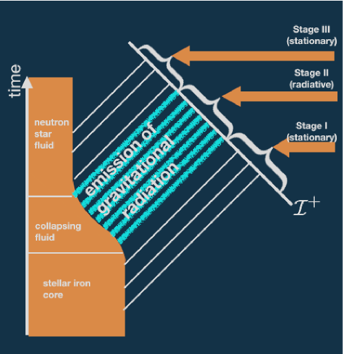
Figure 1: Example for a stationary-to-radiative-to-stationary three-stage model of a stellar core-collapse described in the text. Null infinity is the surface $\mathcal{I}^{+}$. The time axis measures the Newtonian time $t$ along the centre of mass of the stellar fluid.

An exemplary system with a Newtonian limit is a core-collapse supernova scenario, where the initial system, say (I), is an degenerated iron core of an isolated star of mass $M<8M_{\odot}$ (see e.g., (Muell, ; review2, , for an astrophysical review)(Siebel, , in the context of the Bondi-Sachs formalism) and (cerda, , where a star collapses to a black hole via formation of an intermediate (proto-)neutron star (see Figure 1)). The state (I) is ‘clearly’ Newtonian as can be seen by calculating the relevant compactness $C=GM/(c^{2}R)$ of the object, i.e., $C\lesssim 10^{-6}$. The iron-core collapses due to the lack of radiation pressure, caused by the stopping of the nuclear fusion in its centre, to balance the gravity of the fluid. During the collapse phase, (II), of the fluid, gravitational waves are in general emitted from the region where the fluid resides. This is because the collapsing fluid behaves to lowest order as a time-varying quadrupole since the initial model (I) is in general rotating. The final remnant of stage (III) after the collapse is a proto-neutron star of mass $M\lesssim 1.4M_{\odot}$, which is a weak relativistic system where $C\sim 10^{-1}$. In this example, the physically investigated system gives rise to a space-time that does not have “holes” in the sense required by Jürgen (GO, , see Sec. 3). That is, space-time has a compact space containing the stellar fluid and an empty region commencing at the boundary of the fluid.

Since all of the mass is confined to a compact space, it is possible to single out a centre-of-mass world line of the fluid. It is thus natural to choose freely falling (Fermi) observers Manasse along this world line, and choose the outgoing null cones emanating from this world line to define a one-parametric family of Bondi-Sachs metrics $g_{ab}(\lambda)$ (such a construction is demonstrated in the axisymmetric vacuum case in vertex ). Studying the time evolution of $g_{ab}(\lambda)$ from stage (I) via the radiative period (II) to the final stage (III) has mainly been done numerically, because on the one hand the equation of state for the fluid matter is in general provided in tabular form, while on the other hand the underlying Einstein-fluid equations are highly nonlinear. However, the numerical solution provides an answer to Jürgen’s question stated above if $\lambda=0$ is chosen for the numerical solution of the one-parametric family of metrics $g_{ab}(\lambda)$.

Despite the problems of nonlinearity and the issue with the equation of state, Winicour is able to make qualitative statements on the evolution of the initial data. But, before a numerical study can be made, the initial data at stage (I) for the Bondi-Sachs metric at some retarded time $u=0$ must be provided. This requires the ‘correct’ determination of the gravitational shear $\sigma$ for the Newtonian system in the (stationary) stage (I). Winicour’s two main articles newt1 and newt2 deal with this question. For its answer, the following assumptions on the Newtonian initial model at stage (I) are made: (i) the fluid is a perfect fluid with matter density $\varrho$ and an equation of state $p(\varrho,\lambda)$, (ii) $w^{i}$, the three-dimensional velocity field of the matter, (iii) $\Phi$, there is a Newtonian gravitational (connection) potential, (iv) the matter is coupled with the connection potential via the Poisson equation, and (v) the (non-relativistic) Euler equations.

7 Opening up light cones—part II

Before discussing the $\lambda$-families of Bondi-Sachs metrics $g_{ab}(\lambda)$, it is worth looking at how a one-parametric family $\eta_{ab}(\lambda,x^{c})$ of the Minkowski metrics in standard Cartesian coordinates $x^{a}=(t,x^{i})$,

$$\eta_{ab}(\lambda,x^{a}){\mathbf{d}}x^{a}\otimes{\mathbf{d}}x^{b}=\mathbf{d}t\otimes\mathbf{d}t-\lambda\delta_{ij}\mathbf{d}x^{i}\otimes\mathbf{d}x^{j}\;\;,$$ (17)

gives rise to a flat space version of a family of Bondi-Sachs metrics $\eta_{ab}(\lambda,y^{a})$ with Bondi-Sachs coordinates $y^{a}$. We denote with $t_{a}=t_{,a}$ the covector of the surfaces of constant time $t$. The limit of (17) for $\lambda=0$ provides an empty Newtonian space-time structure with

$$g_{ab}=t_{a}t_{b}\;\;,\;\;\lambda g^{ab}=-\delta^{a}_{\phantom{a}i}\delta^{b}_{\phantom{a}j}\delta^{ij}\;\;,$$

where the second of the two equations defines Jürgen’s spatial metric (GO, , p. 4),

$${h^{ab}:=-\lim_{\lambda\rightarrow 0}(\lambda g^{ab})}\;.$$

Introduction of $r^{2}=\delta_{ij}x^{i}x^{i}$, allows us to define the scalar field

$$u=t-\lambda^{1/2}r(x^{i})=t-\lambda^{1/2}\big{[}(x^{1})^{2}+(x^{2})^{2}+(x^{3})^{2}\big{]}^{1/2}\;,$$

which corresponds to the special relativistic retarded time $u$, if $\lambda=1$, and to the Newtonian ‘absolute time’, if $\lambda=0$. The gradient to the surfaces $u=const$ is

$$k_{a}=u_{,a}=(1,-\lambda^{1/2}r_{i})\;\;,\;\;r_{i}:=r_{,i}\;\;.$$ (18)

The squared norm of $k_{a}$ vanishes with respect to $\eta_{ab}(\lambda,x^{a})$, thus hypersurfaces $u=const$ are null hypersurfaces. In fact, they are light cones with respect to the (straight) world line $c(t)$ passing through all of the points where $x^{i}=0$ in the hyperplanes $t=const$. The function $r$ measures the distance between the vertex of a given cone $u=0$ and points on this respective cone. The three-dimensional vector $r_{i}$ measures the direction cosines with respect to a parallel propagated frame along $c(t)$. As for the relation $x^{i}=rr^{i}$, it is useful to parameterize $r^{i}=r^{i}(y^{A})$ by two angular coordinates $y^{A}$ that are constant along the generators of the cone. Then $y^{A}$ measure the direction angles of light rays emanating from the vertex along the light cone $u=0$. The ‘propagation velocity’ of light along these rays is $\lambda^{-1/2}$. Now, consider one arbitrary light cone $u=0$ at proper time $t=0$ on $c(t)$. Letting $\lambda\rightarrow 0$, we observe in the behaviour of the tangent vector (18) the ‘opening up’ of the light cones mentioned in Jürgen’s introduction. In this limit, $k_{a}\rightarrow t_{a}$, and $r$ measures the space-like distance in the hyperplane $t=0$ with respect to the point $x^{i}=0$, while $y^{A}$ measure spherical angles with respect to the origin $x^{i}=0$.

A one-dimensional family of flat space Bondi-Sachs metrics $\eta_{ab}(\lambda,y^{A})$ along a world line $c(t)$ is found by a simple coordinate transformation of (17) to null polar coordinates $y^{a}=(u,y^{1}=r,y^{A})$, so that

$$\eta_{ab}(\lambda,y^{a}){\mathbf{d}}y^{a}\otimes{\mathbf{d}}y^{b}={\mathbf{d}}u\otimes{\mathbf{d}}u+2\lambda^{1/2}{\mathbf{d}}u\otimes{\mathbf{d}}r-\lambda r^{2}q_{AB}(y^{A}){\mathbf{d}}y^{A}\otimes{\mathbf{d}}y^{B}\;,$$ (19)

where $q_{AB}(y^{C})=r^{i}_{,A}r^{j}_{,B}\delta_{ij}$ is the unit round sphere metric. We take $y^{A}$ to be the standard spherical angles $y^{A}=(\theta,\phi)$ such that $q_{AB}=\mathrm{diag}(1,\sin^{2}\theta)$. The metric (19) also shows in the limit $\lambda\rightarrow 0$ that

$$\eta_{ab}(\lambda,y^{a})|_{\lambda=0}=u_{,a}u_{,b}=t_{a}t_{b}\;\;,\;\;h^{ab}=-\delta^{a}_{r}\delta^{b}_{r}-\frac{1}{r^{2}}\delta^{a}_{A}\delta^{b}_{B}q^{AB}(y^{C})\;,$$ (20)

where $q^{AB}$ is the inverse metric of the unit sphere $q^{AB}=\mathrm{diag}(1,\sin^{-2}\theta)$, and we adopted Jürgen’s notation for the inverse spatial metric $h^{ab}$.

8 One-parametric families of Bondi-Sachs metrics $g_{ab}(\lambda,y^{c})$

For the investigation of the Newtonian limit of an Einstein-fluid system, the above construction needs to be done at the centre-of-mass world line of the initial model at stage (I). The regularity requirements of the metric along the centre-of-mass world line imposed by a freely falling observer introduces constraints on the metric at the vertices of the null cones that have to be maintained throughout the evolution of the system from stage (I) to stage (III). As such, the boundary conditions are fixed at the origin of the system, which is contrary to fixing the boundary conditions at infinity as proposed by Jürgen (GO, , see Theorem 1 and the conjecture in Sec. 3). The reason for the former is that the Einstein equations in their Bondi-Sachs formulation are integrated along the null rays emanating from the vertex, and the vertices of the null cones must follow a regular world line. Moreover, setting up a Bondi evolution at null infinity is ill-defined as it requires data, the news function $N:=\frac{1}{2}\sigma_{,u}$, in the future because $N$ is a retarded time derivative.

A one-parametric family of Bondi-Sachs metrics $g_{ab}(\lambda,y^{a})$ is given by newt1 ; newt2 :

$$g_{ab}(\lambda,y^{a}){\mathbf{d}}y^{a}\otimes{\mathbf{d}}y^{b} = \Big{(}\frac{V}{r}e^{2\lambda\beta}-\lambda^{2}r^{2}h^{AB}U_{A}U_{B}\Big{)}{\mathbf{d}}u\otimes{\mathbf{d}}u+2\lambda^{1/2}e^{2\lambda\beta}{\mathbf{d}}r\otimes{\mathbf{d}}u$$ (21)

$$+2\lambda^{3/2}r^{2}U_{A}{\mathbf{d}}x^{A}\otimes{\mathbf{d}}u-\lambda r^{2}h_{AB}{\mathbf{d}}y^{A}\otimes{\mathbf{d}}y^{B}\;,$$

where the metric functions $V$ and $h_{AB}$ are represented by

$$V=r+\lambda W\;\;,\;\;h_{AB}=q_{AB}+\lambda\gamma_{AB}\;,$$ (22)

so that, if $W=U_{A}=\gamma_{AB}=0$, the Minkowski metric (19) is obtained. The $\lambda$-factors in (21) are chosen such that the Einstein equations ensure a smooth limit for the fields $\beta,W,U_{A}$ and $\gamma_{AB}$ at $\lambda=0$. This partially answers Jürgen’s (handwritten) question on the differentiability for $\lambda=0$. The conformal metric $h_{AB}$ has the determinant of the unit sphere $\det(h_{AB})=\det(q_{AB})=\sin^{2}\theta$. Setting $\lambda=1$ in (21) yields the standard form of the Bondi-Sachs metric Bondi ; Sachs ; BSscolar . The symmetric $2-$tensor $\gamma_{AB}$ is transverse-traceless and, due to the choice of coordinates, it gives rise to the shear tensor $c_{AB}$ of the outgoing null cones with tangent vector $k^{a}$,

$$c_{AB}:=\gamma_{AB,r}=\lambda^{-1}h_{AB,r}\;\;.$$ (23)

The gravitational shear tensor incorporates the $\oplus$ and $\otimes$ polarizations of the gravitational waves (see, e.g., Thorne for a relation to the ‘usual’ post-Newtonian formulation). Given a complex dyad $m^{A}$ defined via

$$h_{AB}m^{A}\bar{m}^{B}=1\;\;;\;\;h_{AB}m^{A}m^{B}=0\;\;;\;\;h_{AB}=2m_{(A}\bar{m}_{B)}\;,$$

the two degrees of freedom of $c_{AB}$ are most conveniently expressed through a complex spin-weight-two scalar field,

$$\sigma=m^{A}m^{B}c_{AB}\;\;,$$ (24)

because the decomposition of $c_{AB}$ in terms of $m_{A}$ is

$$c_{AB}=\sigma\bar{m}_{A}\bar{m}_{B}+\bar{\sigma}m_{A}m_{B}\;\;.$$ (25)

The variable $\sigma$ is one of the Newman-Penrose connection coefficients, and it is the free gravitational datum of the characteristic initial value problem. Considering the Newtonian limit of the curvature, $\sigma$ determines part of the Weyl tensor

$$m^{A}m^{B}C_{rArB}\Big{|}_{\lambda=0}=-\frac{1}{2}(r^{2}\sigma)_{,r}\;\;.$$ (26)

As this part of the Weyl tensor corresponds to the Newman-Penrose scalar $\Psi_{0}$, which represents the incoming radiation of a system, the ‘correct’ choice for the free data has an important bearing on the existence of a Newtonian limit given a one-parametric family of Bondi-Sachs metrics $g_{ab}(\lambda,y^{a})$. This means that, although $\sigma$ is, in principle, arbitrary—like, for example, setting the initial shear to zero at some time $u=0$—this will introduce incoming radiation to the system newt1 (see e.g. BKS ; BoostedKerr for details on ingoing radiation in Schwarzschild/Kerr space-times).

9 The Newtonian limit of a family of null cones

Due to the implications of the twice contracted Bianchi identities and due to the requirement of the regularity conditions imposed at the vertices of the null cones, only six of the ten Einstein equations need to be considered for the Bondi-Sachs metric (21) (see e.g. BSscolar for demonstration). Four of these six equations are hypersurface equations not containing any time-derivatives, and the remaining two equations describe the retarded time-evolution of $\sigma$. Only the general structure of these equations is required here, not their particular form.

9.1 Consequences of the hypersurface equations

Two of the four hypersurface equations are second-order differential equations, and it is illustrative to rewrite them in terms of four first-order equations. Moreover, we also list the definition of the shear as one of the hypersurface equations. The final hypersurface equations to be considered are:

$$h_{AB,r} = F^{(0)}_{AB}(\sigma)\;\;;$$ (27a)

$$\beta_{,r} = F^{(1)}(\sigma,h_{AB},T_{rr})\;\;;$$ (27b)

$$Q_{A,r} = F^{(2)}_{A}(\sigma,h_{AB},\beta,T_{rA})\;\;;$$ (27c)

$$h_{AB}U^{B}_{,r} = \frac{1}{r^{4}}e^{-2\lambda\beta}Q_{A}\;\;;$$ (27d)

$$W_{,1} = F^{(3)}(\sigma,h_{AB},\beta,Q_{A},U^{A},T_{ru})\;\;,$$ (27e)

where $U^{A}=h^{AB}U_{B}$, and the placeholders $F^{(\bullet)}_{\bullet}$ are in general nonlinear functions of the arguments. The right-hand side of (27a) follows from the definitions (23)-(25). The four equations (27c) and (27d) are the result of casting the respective second-order differential equations of the corresponding Einstein equations into first-order equations. The components $T_{ra}$ are the components of the energy-momentum tensor of a perfect fluid with an isotropic pressure $p$ of the form:

$$T_{ab}=(\varrho+\lambda p)w_{a}w_{b}-\lambda pg_{ab}\;\;,w_{a}=t_{a}+\lambda v_{a}\;\;,$$ (28)

where $v_{a}$ is the $4-$velocity of the fluid with the Newtonian limit ${v^{a}=(1,V^{r},V^{A})}$ in polar coordinates for $\lambda=0$. Equations (27) show that, if the values of the $h_{AB}$, $\beta$, $Q_{A}$, $U^{A}$ and $W$ are known at the vertices $r=0$, then this provides knowledge of $\sigma$ and $T_{ra}(\varrho,v_{a})$ everywhere on a null cone $u=u_{0}$; the equations (27) can then be solved in a hierarchical manner. For example, given $\sigma$ on a cone $u_{0}$ and initial values for $h_{AB}$ at the vertex, (27a) can be solved for $h_{AB}$ on the entire cone $u_{0}$; then, with the so-obtained $h_{AB}$, $\beta$ can be found on the cone $u_{0}$ using (27b), provided we have knowledge of $T_{rr}$ on all of $u_{0}$ and an initial value for $\beta$. This hierarchical scheme proceeds until $W$ is found after integration of (27e). In particular, we note that $W$ is completely determined by the shear $\sigma$, the fluid data $\varrho$ and $v_{a}$, that is

$$W=W(\sigma,\varrho,V_{r},V_{A})\;\;.$$

Turning the argument around, this also implies that any restriction on $W$ must necessarily restrict the gravitational shear $\sigma$, meaning

$$\sigma=\sigma(W,\varrho,V_{r},V_{A})\;\;,$$

provided the hierarchy (27) can be inverted in a given way. Indeed, considering Eqs. (27) for the limit $\lambda=0$, Winicour has shown newt1 ; newt2 that there exists a scalar field $\Phi^{*}$ given by

$$\Phi^{*}=\frac{W}{2r}\Big{|}_{\lambda=0}+\beta|_{\lambda=0}\;,$$ (29)

that is $O(r)$ at the vertices $r=0$, and which allows for such an inversion. On top of that, this scalar field has the desired decomposition of the connection (GO, , Eq. (39)),

$$\Gamma^{a}_{bc}=\Big{(}\stackrel{{\scriptstyle o}}{{\Gamma}}\!^{a}_{cd}-\lambda t_{b}t_{c}g^{ae}\Phi^{*}_{,e}\Big{)}\Big{|}_{\lambda=0}\;,$$ (30)

into the connection of a pure field of inertia $\stackrel{{\scriptstyle o}}{{\Gamma}}\!^{a}_{bc}$ (in spherical coordinates $r$, $\theta$ and $\phi$) and a space-like vectorial gravitational field $g^{ae}\Phi^{*}_{,e}$ in the Newtonian limit $\lambda=0$, which also obeys the Poisson equation in the limit $\lambda=0$. Denoting with $Y_{lm}(y^{A})$ the standard spherical harmonics, $\Phi^{*}$ differs from the usual Newtonian potential $\Phi$ by monopole-dipole terms:

$$\Phi^{*}=\Phi+aY_{00}(y^{A})+r[a_{-1}Y_{1-1}(y^{A})+a_{0}Y_{10}(y^{A})+a_{1}Y_{11}(y^{A})]\;,$$ (31)

which vanish at infinity through a solution of the Laplace equations. Here, $\Phi$ is a solution of the Poisson equation of the Newtonian initial model. By a rather tedious inversion of the hierarchy (27), Winicour has shown that the modified Newtonian potential relates to a shear-like term,

$$q^{A}q^{B}\eth_{A}\eth_{B}\Phi^{*}=-\frac{1}{2}(r^{2}\sigma)_{,r}\Big{|}_{\lambda=0}\;,$$ (32)

where ${q^{A}=2^{-1/2}(1,i\sin^{-1}\theta)}$ and $\eth_{A}$ is the covariant derivative of the unit round sphere metric.

Relation (32) is in principle the answer to Winicour’s question (1) and it gives rise to a ‘simple’ algorithm to determine the initial data, i.e., $\sigma$, for a quasi-Newtonian system at a null cone with a Newtonian limit for $\lambda=0$: first, the Poisson equation for the potential $\Phi$ is solved for the Newtonian system; second, the gravitational shear $\sigma$ is determined from (31) and (32), where the boundary conditions are fixed at the origin. Note that, as $\sigma$ is a complex field of spin-weight-two, it can always be written as $\sigma=q^{A}q^{B}\eth_{A}\eth_{B}\Sigma$, where $\Sigma$ is a complex scalar field of spin-weight-zero. The real and imaginary parts of $\Sigma$ are called the electric and magnetic parts of $\Sigma$, respectively. This nomenclature is adopted from the electric/magnetic decomposition of the Faraday tensor of the electromagnetic field, and corresponds to a curl/gradient decomposition of tensor fields on a sphere (see e.g. skypattern for a related discussion with regard to gravitational waves).

9.2 Consequences of the evolution equations

Considering the evolution equation of the Bondi-Sachs metric, which schematically reads:

$$2(r^{2}\sigma)_{,u}=\lambda(r^{2}\sigma)_{,r}+F^{(4)}(\lambda,\beta,h_{AB},W,U^{A},Q_{A},\varrho,p,v_{a})\;\;,$$ (33)

Winicour shows that $\Sigma$ (and consequently also $\sigma$) must be purely electric in order to provide initial data on the null cone that are smooth in $\lambda$. To some extent this observation also gives a further answer to Jürgen’s question (5b), indicating that the differentiability in $\lambda$ is necessary to obtain a bona fide Newtonian limit of his “Frame Theory”.

The answer to Winicour’s second question (2) on the validity of the initial data with regard to its Newtonian limit during a retarded time-evolution requires consideration of the evolution equation (33) and the local conservation law of energy-momentum, $\nabla_{a}T^{a}_{\phantom{a}b}=0$, at leading order in $\lambda$. Energy-momentum conservation in the limit $\lambda=0$ ensures that $\varrho_{N}$ and $v^{i}_{N}$ remain valid throughout the time interval $[u_{0},u_{1}]$. To investigate the time-evolution of $\sigma_{N}$ for the evolution on the retarded time interval $[u_{0},u_{1}]$, all fields ${\mathcal{F}\in\{\beta,h_{AB},U^{A},V,\varrho,p,v_{a}\}}$ are assumed to have a smooth $\lambda-$expansion of the type $\mathcal{F}(\lambda)=\sum_{n}\mathcal{F}_{(n)}\lambda^{n}$. Inserting these expansions into the evolution equation (33) yields an iterative scheme, where the retarded time-derivative of the shear $\sigma_{(n)}$ is determined by the $\sigma_{(n-1)}$ coefficient. The $\sigma_{(1)}$ coefficient is unconstrained and may be used to fix the initial data on the cone $u=u_{0}$. The successive determination of the $\sigma_{(n)}$ from a Newtonian model $(\Phi,\varrho,p(\varrho),V_{r},V_{A})$ provides the gravitational initial data for the Bondi-Sachs system, preserving the Newtonian limit for $\lambda=0$. Proper determination of the $\sigma_{(n)}$’s is crucial for ruling out, in Jürgen’s words, “…incoming fields from the exterior. (GO, , p. 9)”. The algorithm to calculate $\sigma_{(n)}$ up to $n=2$ is given in newt2 , and an example for Newtonian dust at $\lambda=0$ can be found in dust .

We finally note an important observation regarding the $\lambda$-expansion of $\mathcal{F}$: since all fields become $\lambda$-dependent for $u>u_{0}$ during the evolution of the centre-of-mass world line of the Newtonian system, this system will in general move away from the geodesic along which the null cones of the Bondi-Sachs metric are constructed. This is because of the $\lambda$-dependence of the pressure, whose gradient introduces an acceleration towards fluid elements at the origin of the geodesic of the Newtonian theory at $\lambda=0$.

10 Closing remarks

Jürgen conjectured (GO, , Sec. 3) that space-times that are asymptotically flat at space-like and null infinity have a Newtonian limit. This fixes the boundary conditions of the fields at infinity. Asymptotic flatness at null infinity implies the peeling property Sachs of the Weyl tensor $C_{abcd}$ in the limit $r\rightarrow\infty$. The ten independent components of $C_{abcd}$ are most conveniently expressed in terms of the five complex Newman-Penrose Weyl scalars $\Psi_{n},n\in\{0,...4\}$ NP ; NPscolar , and the peeling property of asymptotically flat space-times is given by $\Psi_{n}(y^{a})=\Psi^{(0)}_{n}(u,y^{A})/r^{5-n}+O(r^{-6})$. Winicour, however, fixed the boundary conditions of the fields at a geodesic inside a Newtonian matter distribution. This is necessary to obtain a well-defined characteristic initial value formulation. In turn, no conditions at null infinity can be fixed. Surprisingly, further investigations of Winicour and collaborators show, for an exemplary system with a Newtonian limit at $\lambda=0$, that the Weyl tensor does not need to have the peeling property. Especially due to the presence of a logarithmic term in $\sigma$ implied by such a Newtonian limit, the asymptotic behaviour of the Weyl tensor is spoiled quadPRL , as it does not behave as $C_{abcd}=O(r^{-1})$, as implied by the peeling theorem, but it behaves as $O(r^{-1}\ln r)$. Thus, peeling cannot be recovered, but it is possible to establish a weaker version of the peeling theorem, where both the electric and the magnetic parts of the Weyl tensor are $O(r^{-1})$ in the limit $r\rightarrow\infty$ logScri . Nevertheless, the famous Einstein quadrupole formula is unaffected by this logarithmic behaviour and has a Newtonian limit for $\lambda=0$ quad ; quadPRL . Although, the finding of logarithmic terms at null infinity came as a surprise when mapping a Newtonian system onto a null cone of a quasi-Newtonian relativistic system, logarithmic terms can also be found by considering the global asymptotics of the characteristic initial value formulation of General Relativity poly1 ; christ . Indeed, further investigations poly1 showed the existence of an entire ‘zoo’ of polyhomogeneous space-times (i.e., space-times where the Weyl tensors are $O(r^{-k}\ln^{m}r)$ with with $k,m\geq 1$), and whose mathematical meaning is not yet fully understood. One might speculate that some of them relate to higher-order corrections to the null cone initial data when Newtonian models of a Newton-Cartan theory at $\lambda=0$ are mapped onto a null cone.

Jürgen raises some doubts (“For Einstein’s Theory many asymptotic flatness conditions were proposed […] but their suitability for non stationary space-times is still in doubt (GO, , p. 9)”) about whether asymptotic flatness for isolated systems at null infinity is in fact a completed chapter. Winicour’s approximation model for a one-parametric family of Bondi-Sachs metrics $g_{ab}(\lambda)$ with a Newtonian system at $\lambda=0$ together with the zoo of polyhomogeneous space-times is proof that Jürgen’s doubt on asymptotically flat space-times is still standing. In particular, Jürgen’s advice to not take for granted generally imposed assumptions (as noted in GO “…textbook and monographs suggest the existence of a well-understood [Newtonian] limit $(\rightarrow)$ … (GO, , p. 2)”) should be taken as a motto for any scientist, not only working in General Relativity.

Biography: Jürgen Ehlers

A biography of Jürgen Ehlers was published in Gen. Relativ. Gravit. 41, 1899 (2009), in the form of the obituary reprinted from the Biennial Report 2006/2007 of the Albert Einstein Institute.

Acknowledgements We wish to thank Malcolm MacCallum for inviting this editorial note and for constant assistance. In particular, TM thanks Malcolm MacCallum for help on some subtle grammatical issues as well as ‘false friends’ appearing in a first draft of the translation of GO . We thank Frank Steiner for valuable remarks.

References

-
(1)
Ehlers, J., Über den Newtonschen Grenzwert der Einsteinschen Gravitationstheorie, in Grundlagenprobleme der modernen Physik, ed J. Nitsch, Mannheim, Wien, Zürich: Bibliographisches Institut (1981);
translation to appear in: Gen. Relativ. Gravit. 51 163 (2019)
- (2) Alles, A., Buchert, T., Al Roumi, F., Wiegand, A., Lagrangian theory of structure formation in relativistic cosmology. III. gravitoelectric perturbation and solution schemes at any order, Phys. Rev. D 92, 023512 (2015) arXiv:1503.02566
- (3) Al Roumi, F., Buchert, T., Wiegand, A., Lagrangian theory of structure formation in relativistic cosmology. IV. Lagrangian approach to gravitational waves, Phys. Rev. D 96, 123538 (2017) arXiv:1711.01597
- (4) Bondi, H., van der Burg, M.G.J., Metzner, A.W.K., Gravitational Waves in General Relativity. VII. Waves from Axi-Symmetric Isolated Systems, Proceedings of the Royal Society of London Series A 269, 21 (1962)
- (5) Buchert, T., Lagrangian perturbation approach to the formation of large-scale structure, in: International School of Physics Enrico Fermi, Course CXXXII: Dark Matter in the Universe, Varenna 1995, eds.: S. Bonometto, J. Primack, A. Provenzale, IOP Press Amsterdam, 543-564 (1996) arXiv:astro-ph/9509005
- (6) Buchert, T., An exact Lagrangian integral for the Newtonian gravitational field strength, Phys. Lett. A 354, 8 (2006) arXiv:gr-qc/0508059
- (7) Buchert, T., Toward physical cosmology: focus on inhomogeneous geometry and its non-perturbative effects, Class. Quant. Grav. 28, 164007 (2011) arXiv:1103.2016
- (8) Buchert, T., Ehlers J., Lagrangian theory of gravitational instability of Friedmann-Lemaître cosmologies—second-order approach: an improved model for non-linear clustering, Mon. Not. Roy. Astr. Soc. 264, 375 (1993) ADS
-
(9)
Buchert, T., Ehlers J., Averaging inhomogeneous Newtonian cosmologies,
Astron. Astrophys. 320, 1 (1997) arXiv:astro-ph/9510056 - (10) Buchert, T., Götz, G., A class of solutions for self-gravitating dust in Newtonian gravity, J. Math. Phys. 28, 2714 (1987)
- (11) Buchert, T., Ostermann, M., Lagrangian theory of structure formation in relativistic cosmology I: Lagrangian framework and definition of a nonperturbative approximation, Phys. Rev. D 86, 023520 (2012) arXiv:1203.6263
-
(12)
Cerdá-Durán, P., DeBrye, N., Aloy, M.A., Font, J.A., Obergaulinger, M.,
Gravitational Wave Signatures in Black Hole Forming Core Collapse,
The Astrophysical Journal 779, L18 (2013) ADS - (13) Cerdá-Durán, P., Elias-Rosa, N., Neutron stars formation and Core Collapse Supernovae, Astrophysics and Space Science Library 457 1, Springer Nature Switzerland (2018) arXiv:1806.07267
- (14) Christodoulou, D., The global initial value problem in General Relativity, in Proceedings of the Ninth Marcel Grossman Meeting on General Relativity, ed V. Gurzadyan, R. Jantzen and R. Ruffini, World Scientific, Singapore, pp. 44–54 (2002)
- (15) Chruściel, P.T., MacCallum, M.A.H., Singleton, D.B., Gravitational Waves in General Relativity. XIV: Bondi Expansions and the “Polyhomogeneity” of Scri, Phil. Trans. Roy. Soc. Lond. A 350, 19950004 (1995) arXiv:gr-qc/9305021
-
(16)
Ehlers, J., Akad. Wiss. Lit. (Mainz); Abh. Math.-Nat. Kl. No. 11, 793 (1961);
translation: Contributions to the relativistic mechanics of continuous media,
Gen. Relativ. Gravit. 25, 1225 (1993) - (17) Ehlers, J., The Newtonian limit of General Relativity, in Classical Mechanics and Relativity: Relationship and Consistency ed G. Ferrarese, pp. 95–106). Napoli, Italy: Napoli–Bibliopolis (1991)
-
(18)
Ehlers, J., Examples of Newtonian limits of relativistic space-times,
Class. Quant. Grav. 14, A119–A126 (1997) - (19) Ehlers, J., Buchert, T., Newtonian cosmology in Lagrangian formulation: foundations and perturbation theory, Gen. Relativ. Gravit. 29, 733 (1997) arXiv:astro-ph/9609036
-
(20)
Ehlers, J., Buchert, T., On the Newtonian limit of the Weyl tensor,
Gen. Relativ. Gravit. 41, 2153 (2009) arXiv:0907.2645 - (21) Ellis, G.F.R., van Elst, H., Cosmological models (Cargèse lectures 1998), Theoretical and observational cosmology, Proceedings of the NATO Advanced Study Institute on Theoretical and Observational Cosmology, Cargèse, France, 1998, ed M. Lachièze–Rey. Boston: Kluwer Academic, NATO science series C, Mathematical and physical sciences, vol. 541, pp. 1–116 (1999) arXiv:gr-qc/9812046
- (22) Van Elst, H., Uggla, C., Lesame, W.M., Ellis, G.F.R., Maartens, R., Integrability of irrotational silent cosmological models, Class. Quant. Grav. 14, 1151 (1997) arXiv:gr-qc/9611002
- (23) Geroch, R., Limits of spacetimes, Comm. Math. Phys. 13(3), 180 (1969)
- (24) Heaviside, O., A gravitational and electromagnetic analogy, The Electrician 31, 281 (part I), 359 (part II) (1893) html online by O. D. Jefimenko
-
(25)
Heilig, U., On the existence of rotating stars in General Relativity,
Comm. Math. Phys. 166, 457 (1995) - (26) Isaacson, R.A., Welling, J.S., Winicour, J.H., Extension of the Einstein Quadrupole Formula, Phys. Rev. Lett. 53, 1870 (1984)
- (27) Isaacson, R.A., Welling, J.S., Winicour, J.H., Gravitational radiation from dust, J. Math. Phys. 26, 2859 (1985)
- (28) Jantzen, R.T., Carini, P., Bini, D., The many faces of gravitoelectromagnetism, Annals of Physics 215, 1 (1992) arXiv:gr-qc/0106043
-
(29)
Kofman, L., Pogosyan, D., Dynamics of gravitational instability is nonlocal,
Astrophys. J. 442, 30 (1995) arXiv:astro-ph/9403029 - (30) Levin, J., Scannapieco, E., Silk, J., The topology of the universe: the biggest manifold of them all, Class. Quant. Grav. 15, 2689 (1998) arXiv:gr-qc/9803026
- (31) Lottermoser, M., A convergent post-Newtonian approximation for the constraints in General Relativity, Ann. Inst. Henri Poincaré 57, 279 (1992)
- (32) Mädler, T., Müller, E., The Bondi-Sachs metric at the vertex of a null cone: axially symmetric vacuum solutions, Class. Quant. Grav. 30, 055019 (2013) arXiv:1211.4980
- (33) Mädler, T., Winicour, J.H., Bondi-Sachs Formalism, Scholarpedia 11(12), 33528 (2016) arXiv:1609.01731
- (34) Mädler, T., Winicour, J.H., The sky pattern of the linearized gravitational memory effect, Class. Quant. Grav. 33, 175006 (2016) arXiv:1605.01273
- (35) Mädler, T., Winicour, J.H., Radiation memory, boosted Schwarzschild spacetimes and supertranslations, Class. Quant. Grav. 34, 115009 (2017) arXiv:1701.02556
- (36) Mädler, T., Winicour, J.H., Boosted Schwarzschild Metrics from a Kerr-Schild Perspective, Class. Quant. Grav. 35, 035009 (2018) arXiv:1708.08774
-
(37)
Mädler, T., Winicour, J.H., Kerr black holes and nonlinear radiation memory,
Class. Quant. Grav. 36, 095009 (2019) arXiv:1811.04711 - (38) Manasse, F.K., Misner, C.W., Fermi normal coordinates and some basic concepts in differential geometry, J. Math. Phys. 4, 735 (1963)
-
(39)
Müller, B., The Status of Multi-Dimensional Core-Collapse Supernova Models,
Pub. Astronom. Soc. Aus. 33, e048 (2016) arXiv:1608.03274 - (40) Newman, E.T., Penrose, R., An Approach to Gravitational Radiation by a Method of Spin Coefficients, J. Math. Phys. 3, 566 (2004)
- (41) Newman, E.T., Penrose, R., Spin-coefficient formalism, Scholarpedia 4(6), 7445 (2009)
- (42) Oliynyk, T.A., Schmidt, B., Existence of families of space-times with a Newtonian limit, Gen. Relativ. Gravit. 41, 2093 (2009)
- (43) Penrose, R., Asymptotic Properties of Fields and Space-Times, Phys. Rev. Lett. 10, 66 (1963)
- (44) Rendall, A.D., The Newtonian limit for asymptotically flat solutions of the Vlasov-Einstein system, Commun. Math. Phys. 163, 89 (1994) arXiv:gr-qc/9303027
- (45) Sachs, R.K., Gravitational Waves in General Relativity. VIII. Waves in Asymptotically Flat Space-Time, Proceedings of the Royal Society of London Series A 270, 103 (1962)
- (46) Schutz, B., Report on the symposium ‘Radiative space-times and approximation methods’, held during the 11th International Conference on General Relativity and Gravitation, Stockholm, Sweden, 6–12 July (1986) online on Google Scholar
- (47) Siebel, F., Font, J.A., Müller, E., Papadopoulos, P., Axisymmetric core collapse simulations using characteristic numerical relativity, Phys. Rev. D 67, 124018 (2003) arXiv:gr-qc/0301127
- (48) Steiner, F., Do Black Holes exist in a finite Universe having the topology of a flat 3–Torus? Ulmer Seminare 2016/2017, eds. W. Arendt et al., Heft 20, 331–351 arXiv:1608.03133
- (49) Tamburino, L.A., Winicour, J.H., Gravitational Fields in Finite and Conformal Bondi Frames, Phys. Rev. 150, 1039 (1966)
- (50) Thorne, K.S., The theory of gravitational radiation—an introductory review, in Gravitational radiation, Proceedings of the Advanced Study Institute, Les Houches, Haute-Savoie, France, June 2-21, 1982 (A84-35026 16-90), ed N. Deruelle and T Piran, Amsterdam, North-Holland Publishing, pp. 1-57 (1985)
- (51) Winicour, J.H., Newtonian gravity on the null cone, J. Math. Phys. 24, 1193 (1983)
- (52) Winicour, J.H., Null infinity from a quasi-Newtonian view, J. Math. Phys. 25, 2506 (1984)
- (53) Winicour, J.H., The quadrupole radiation formula, Gen. Relativ. Gravit. 19, 281 (1987)
-
(54)
Winicour, J.H., Characteristic Evolution and Matching,
Living Reviews in Relativity 15, 2 (2012) arXiv:0810.1903 - (55) Winicour, J.H., Logarithmic asymptotic flatness, Foundations of Physics 15, 605 (1985)