Measurement of properties of $\PBzs\to\MM$ decays and search for $\PBz\to\MM$ with the CMS experiment

Abstract

Results are reported for the $\PBzs\to\MM$ branching fraction and effective lifetime and from a search for the decay $\PBz\to\MM$. The analysis uses a data sample of proton-proton collisions accumulated by the CMS experiment in 2011, 2012, and 2016, with center-of-mass energies (integrated luminosities) of 7 (5), 8 (20), and 13 (36). The branching fractions are determined by measuring event yields relative to $\PBp\to\PJGy\PKp$ decays (with $\PJGy\to\Pgmp\Pgmm$), which results in the reduction of many of the systematic uncertainties. The decay $\PBzs\to\MM$ is observed with a significance of 5.6 standard deviations. The branching fraction is measured to be $\mathcal{B}(\PBzs\to\MM)=[2.9\ \pm 0.7(\text{exp})\pm 0.2(\text{frag})]\times 10^{-9}$, where the first uncertainty combines the experimental statistical and systematic contributions, and the second is due to the uncertainty in the ratio of the  and the  fragmentation functions. No significant excess is observed for the decay $\PBz\to\MM$, and an upper limit of $\mathcal{B}(\PBz\to\MM)<3.6\times 10^{-10}$ is obtained at 95% confidence level. The $\PBzs\to\MM$  effective lifetime is measured to be $\tau_{\Pgmp\Pgmm}=1.70\,^{+0.61}_{-0.44}\unit{ps}$. These results are consistent with standard model predictions.

0.1 Introduction

Leptonic meson decays offer excellent opportunities to perform precision tests of the standard model (SM) of particle physics because of minimal hadronic uncertainties in the theoretical predictions [1, 2, 3, 4, 5]. In the SM, the decays $\PBzs\to\MM$ and $\PBz\to\MM$ proceed only via loop diagrams and are also helicity suppressed, leading to very small expected decay time-integrated branching fractions, $(3.66\pm 0.14)\times 10^{-9}$ and $(1.03\pm 0.05)\times 10^{-10}$, respectively. Theoretical uncertainties in the calculation of these branching fractions have been reduced in recent years as a result of progress in lattice quantum chromodynamics (QCD) [6, 7, 8, 9, 10], in the calculation of electroweak effects at next-to-leading order [2], and in the calculation of QCD effects at next-to-next-to-leading order [3]. Enhanced electromagnetic contributions from virtual photon exchange have been shown [4, 5] to produce larger corrections than previously assumed in the theoretical uncertainties. The $\PBzs\to\MM$ branching fraction has been measured in proton-proton ($\Pp\Pp$) collisions by the CMS, LHCb, and ATLAS Collaborations [11, 12, 13, 14]. For the decay $\PBz\to\MM$, evidence at the three standard deviation level has been obtained by the CMS and LHCb Collaborations in a combined analysis [12] of $\sqrt{s}=7$ and 8data. However, this has not been confirmed by LHCb after incorporating 13data [13], nor by ATLAS [14].

The heavy (${\PB}^{0}_{\mathrm{sH}}$) and light (${\PB}^{0}_{\mathrm{sL}}$) mass eigenstates are linear combinations of the flavor eigenstates, $|{\PB}^{0}_{\mathrm{sL(H)}}\rangle=p|\PBzs\rangle\pm q|\PABzs\rangle$, with the normalization condition $\abs{p}^{2}+\abs{q}^{2}=1$. The decay amplitudes $\hbox{\vbox{\hrule height=0.4pt\kern 2.15277pt\hbox{\kern 0.0pt$A$\kern 0.0pt}}\raisebox{9.0pt}{\scalebox{0.4}{\text{\kern-23.00006pt(}}} \raisebox{9.0pt}{\scalebox{0.4}{\text{\kern 13.00005pt)}}} }_{\kern-2.79996pt\Pgmp\Pgmm}=A(\hbox{\vbox{\hrule height=0.4pt\kern 2.15277pt\hbox{\kern 0.0pt$\PB$\kern 0.0pt}}\raisebox{9.0pt}{\scalebox{0.4}{\text{\kern-18.99995pt(}}} \raisebox{9.0pt}{\scalebox{0.4}{\text{\kern 8.99994pt)}}} }_{\kern-2.79996pt\mathrm{s}}{}^{\kern-1.39998pt0}\to\Pgmp\Pgmm)$, together with $p$ and $q$, are used to define [15] the parameters $\lambda\equiv(q/p)(\overline{A}_{\Pgmp\Pgmm}/A_{\Pgmp\Pgmm})$ and ${\mathcal{A}}_{\Delta\Gamma}^{\Pgmp\Pgmm}\kern-1.99997pt\equiv-2\Re(\lambda)/(1+\abs{\lambda}^{2})$. The SM predicts ${\mathcal{A}}_{\Delta\Gamma}^{\Pgmp\Pgmm}\kern-1.99997pt=+1$, , that only the heavy state, with measured lifetime $\tau_{{\PB}^{0}_{\mathrm{sH}}}=1.615\pm 0.009\unit{ps}$ [16], contributes to the $\PBzs\to\MM$ decay. The $\PBzs\to\MM$ effective lifetime is defined by

$$\tau_{\Pgmp\Pgmm}\equiv\frac{\int_{0}^{\infty}t\,[\Gamma(\PBzs(t)\to\Pgmp\Pgmm)+\Gamma(\PABzs(t)\to\Pgmp\Pgmm)]\,\rd{}t}{\int_{0}^{\infty}[\Gamma(\PBzs(t)\to\Pgmp\Pgmm)+\Gamma(\PABzs(t)\to\Pgmp\Pgmm)]\,\rd{}t},$$ (1)

where $t$ is the proper decay time of the  meson [17]. The effective lifetime is related to the  mean lifetime through [18]

$$\tau_{\Pgmp\Pgmm}=\frac{\tau_{\PBzs}}{1-y_{\mathrm{s}}^{2}}\left(\frac{1+2{\mathcal{A}}_{\Delta\Gamma}^{\Pgmp\Pgmm}\kern-1.99997pt\,y_{\mathrm{s}}+y_{\mathrm{s}}^{2}}{1+{\mathcal{A}}_{\Delta\Gamma}^{\Pgmp\Pgmm}\kern-1.99997pt\,y_{\mathrm{s}}}\right),$$ (2)

where the parameter $y_{\mathrm{s}}\equiv\tau_{\PBzs}\Delta\Gamma_{\mathrm{s}}/2=0.066\pm 0.004$ is defined using the measured  mean lifetime $\tau_{\PBzs}=1.509\pm 0.004\unit{ps}$ and $\PBzs\text{--}\PABzs$ decay width difference $\Delta\Gamma_{\mathrm{s}}\equiv{\Gamma_{\mathrm{s}}}_{\text{L}}-{\Gamma_{\mathrm{s}}}_{\text{H}}=0.088\pm 0.006\mbox{$\,\text{ps}^{-1}$}$ [16]. A first measurement of the effective lifetime, $\tau_{\Pgmp\Pgmm}=2.04\pm 0.44\pm 0.05\unit{ps}$, which is consistent with the SM expectation, has been presented by the LHCb Collaboration [13].

In this paper, we report updated results for the $\PBzs\to\MM$ and $\PBz\to\MM$ branching fractions, as well as a measurement of the $\PBzs\to\MM$ effective lifetime. The data were collected in $\Pp\Pp$ collisions at the CERN LHC, and correspond to integrated luminosities of 5 and 20recorded in 2011 and 2012 at $\sqrt{s}=7$ and 8, respectively, during Run 1 of the LHC, and 36recorded in 2016 at $\sqrt{s}=13\TeV$, during Run 2. Depending on the context, the symbol is used to denote the , , and  mesons and/or the baryon, and charge conjugation is implied throughout, except as noted. The present branching fraction measurements supersede the previous CMS results [11], which used Run 1 data only. The main differences with respect to the previous branching fraction results include the greater statistical precision of the larger data sample, an improved muon identification algorithm, based on a newly developed boosted decision tree (BDT), and better constraints against background contamination in the search for $\PBz\to\MM$. In addition to the BDT used for muon identification, the analysis employs a second BDT in the candidate selection. For clarity we will refer to them as the muon BDT and the analysis BDT. The Run 1 data are reanalyzed using the new muon identification algorithm (with its improved BDT), but the candidate selection incorporates the same analysis BDT as used in the original Run 1 analysis, as described in Ref. [11]. The binning of the analysis BDT discriminator distribution, used for the final result extraction, was modified, based on the best expected performance. For the Run 2 data, a new analysis BDT was developed.

The signal sample consists of candidates constructed from two oppositely charged muons, which are constrained to originate from a common origin and have an invariant mass in the range $4.8<m_{\Pgmp\Pgmm}<6.0\GeV$. Within the signal sample, a signal region defined by $5.20<m_{\Pgmp\Pgmm}<5.45\GeV$ is analyzed only after all analysis procedures have been finalized. The background is estimated from mass sidebands in data and from Monte Carlo (MC) simulation for specific background sources from decays. The main background categories are (1) combinatorial background with two genuine muons from semileptonic decays of separate hadrons (, $\Bz\to\PDstm\Pgmp\nu$), (2) rare decays with two muons (, from $\PB\to{\HepParticle{h}{}{}}\mu\mu$ where ${\HepParticle{h}{}{}}\in\{\PGp,\PK,\Pp\}$), and (3) rare decays with one hadron (, from $\PB\to{\HepParticle{h}{}{}}\mu\nu$) or two hadrons (, from $\PB\to{\HepParticle{h}{}{}}{\HepParticle{h}{}{}}^{(\raisebox{-3.01389pt}{'})}$) misidentified as muons. The combinatorial background affects both $\PBzs\to\MM$ and $\PBz\to\MM$ and is the limiting factor for the measurement of the former. The search for the decay $\PBz\to\MM$, with its smaller expected branching fraction and an expected signal-to-background ratio significantly below one, is additionally affected by rare decays, since background from hadronic $\PB$ decays produces a dimuon invariant mass distribution that peaks underneath the $\PBz\to\MM$ signal. The background from rare decays has only a minor impact on the $\PBzs\to\MM$ results.

Because the mass resolution of the CMS detector has a strong dependence on the pseudorapidity $\eta$ of the muons, the analysis sensitivity benefits from a division of the data sets into channels based on the pseudorapidity $\eta^{\text{f}}_{\mu}$ of the most forward muon of the candidate, where $\abs{\eta^{\text{f}}_{\mu}}=\max(\abs{\eta_{\Pgmp}},\abs{\eta_{\Pgmm}})$. A central and a forward channel are defined for all running periods, with different boundaries for Run 1 and Run 2 because of changing trigger requirements.

A normalization sample based on $\PBp\to\PJGy\PKp$ decays (with $\PJGy\to\Pgmp\Pgmm$) is used in the measurement of the branching fractions. In addition, a control sample based on $\PBzs\to\PJGy\PGf$ decays (with $\PJGy\to\Pgmp\Pgmm$ and $\phi\to\PKp\PKm$) is used to study differences between  and  characteristics (fragmentation, isolation, selection efficiency, etc.) in data and to compare with MC simulation. These samples are reconstructed by adding one or two charged tracks with a kaon mass hypothesis to two oppositely charged muons, requiring the dimuon pair to be consistent with $\PJGy$ meson decay.

The $\PBzs\to\MM$ branching fraction is determined using

$$\mathcal{B}(\PBzs\to\MM)=\frac{N_{\mathrm{S}}}{N_{\text{obs}}^{\PBp}}\,\frac{f_{{\PQu}}}{f_{{\PQs}}}\,\frac{\varepsilon_{\text{tot}}^{\PBp}}{\varepsilon_{\text{tot}}}\,\mathcal{B}(\PBp\to\PJGy\PKp)\,\mathcal{B}(\PJGy\to\Pgmp\Pgmm),$$ (3)

where $N_{\mathrm{S}}$ ($N_{\text{obs}}^{\PBp}$) is the number of reconstructed $\PBzs\to\MM$ ($\PBp\to\PJGy\PKp$) decays, $\varepsilon_{\text{tot}}$ ($\varepsilon_{\text{tot}}^{\PBp}$) is the total signal () efficiency, $\mathcal{B}(\PBp\to\PJGy\PKp)=(1.01\pm 0.03)\times 10^{-3}$ and $\mathcal{B}(\PJGy\to\Pgmp\Pgmm)=(5.96\pm 0.03)\times 10^{-2}$ [16], and $f_{\PQu}/f_{\PQs}$ is the ratio of the  and  fragmentation functions. The value $f_{\PQs}/f_{\PQu}=0.252\pm 0.012\,\text{(exp)}\pm 0.015\,\text{(CMS)}$, a combination [16] with input from measurements by the LHCb [19] and ATLAS Collaborations [20], is used. Beyond the experimental uncertainty from Ref. [16], we assign an additional uncertainty (labeled CMS) by adding in quadrature uncertainties evaluated from the consideration of two other issues. First, we derive an uncertainty of 0.008 from the difference between the value of $f_{\PQs}/f_{\PQu}$ in Ref. [16], obtained at $\sqrt{s}=7\TeV$, and that in Ref. [21], obtained at $\sqrt{s}=13\TeV$. Second, using the parametrization of the transverse momentum () dependence in Ref. [21], we determine a difference of 0.013 between the $f_{\PQs}/f_{\PQu}$ values at the average  of Ref. [21] and the average  of the $\PBzs\to\MM$ candidates in this analysis (see below, Table 0.7). This also covers the substantially smaller  dependence of Ref. [22]. An analogous equation to Eq. (3) is used to determine the $\PBz\to\MM$ branching fraction, where we assume $f_{\PQd}/f_{\PQu}=1$ for the ratio of the  to the  fragmentation functions [16].

The measurement of $\mathcal{B}(\PBzs\to\MM)$ and $\mathcal{B}(\PBz\to\MM)$ is performed with an extended unbinned maximum likelihood (UML) fit, with probability density functions (PDFs) obtained from simulated event samples and data sidebands. For the determination of the $\PBzs\to\MM$ effective lifetime $\tau_{\Pgmp\Pgmm}$, two independent procedures are used. The first is based on a two-dimensional (2D) UML fit to the invariant mass and proper decay time distributions of $\PBzs\to\MM$ candidates. The second is based on a one-dimensional (1D) binned maximum likelihood (ML) fit to the background-subtracted proper decay time distribution obtained with the sPlot [23] method.

The presence of multiple $\Pp\Pp$ interactions in an event is referred to as pileup, whose rate is dependent on the instantaneous luminosity. The average number of reconstructed $\Pp\Pp$ interaction vertices is 8, 15, and 18 for the data collected in 2011, 2012, and 2016, respectively.

0.2 Event simulation

Simulated event samples, produced with MC programs, are used to optimize the analysis selection requirements and to determine efficiencies for the signal, normalization, and control samples. The background shapes of the dimuon invariant mass distribution for rare decays, where one or two charged hadrons are misidentified as muons, are also obtained from simulated event samples. The simulated background decay modes include $\PB\to{\HepParticle{h}{}{}}\mu\nu$, $\PB\to{\HepParticle{h}{}{}}\mu\mu$, and $\PB\to{\HepParticle{h}{}{}}{\HepParticle{h}{}{}}^{(\raisebox{-3.01389pt}{'})}$. For the decay $\PGLb\to\Pp\Pgmm\Pagngm$, the model of Ref. [24], based on QCD light-cone sum rules, is used. In addition, the decay $\PBpc\to\PJGy\PGmp\PGn$ was studied, but is not required for an adequate background description after the full selection has been applied and therefore is not considered in the final analysis.

The simulated event samples are generated with  6.426 [25] for the Run 1 analysis and  8.212 [26] for the Run 2 analysis. In both cases, signal and background events are selected from generic $2\to 2$ QCD processes to provide a complete mixture of gluon fusion, gluon splitting, and flavor excitation production. The analysis efficiency varies for these production mechanisms. For instance, in gluon splitting the two quarks can have a small phase space separation such that a $\PBzs\to\MM$ decay is less isolated than in gluon fusion, for which the two quarks are, to first order, back-to-back in the transverse plane. The mixture in the MC simulation is compared to the mixture in data using the normalization and control samples, and a corresponding systematic uncertainty is assigned. The changing pileup conditions are reflected in the event simulation.

The decay of unstable particles is described using the  [27] program and final-state photon radiation using the  [28, 29] program. The detector response is simulated with  [30].

0.3 The CMS detector

The CMS experiment is based on a general purpose detector designed and built to study physics at the TeV scale. A detailed description of the CMS detector, together with a definition of the coordinate system used and the relevant kinematic variables, can be found in Ref. [31]. For this analysis, the main subdetectors used are the silicon tracker, composed of pixel and microstrip detectors within a 3.8T axial magnetic field, and the muon detector, described below. These detectors are divided into a barrel and two endcap sections.

The silicon tracker detects charged particles within $\abs{\eta}<2.5$. The pixel detector is composed of three layers in the barrel region and two disks located on each side in the forward regions. In total, the pixel detector contains about 66 million $100\mum\times 150\mum$ pixels. Further from the interaction region is a microstrip detector, composed of ten barrel layers, and three inner and nine outer disks on either end of the detector, with strip pitches between 80 and 180$\mum$. In total, the microstrip detector contains around 10 million strips and, together with the pixel detector, yields an impact parameter resolution of about $15\mum$. As a consequence of the high granularity of the silicon tracker and the strong and homogeneous magnetic field, a transverse momentum resolution of about 1.5% [32] is obtained for the muons in this analysis. The systematic uncertainty in the track reconstruction efficiency for charged hadrons is estimated to be 4.0 (2.3)% in Run 1 (Run 2) [32, 33]. In Run 2, the microstrip detector experienced operational instabilities during the initial period of the run, resulting in a significant impact on the trigger efficiency as the level of pileup increased. The Run 2 data are therefore divided into two separate running periods, denoted 2016A and 2016B, of roughly equal integrated luminosity. Separate sets of MC samples are used to describe these periods. Residual differences between the MC simulation and the Run 2 data lead to a systematic uncertainty of $\pm 0.07\unit{ps}$ in the effective lifetime measurement. This uncertainty is estimated from the variation in the  lifetime measured with the  normalization sample in the two running periods and channels. The maximum difference with respect to the result in Ref. [16] is assigned as the systematic uncertainty. The uncertainties due to the residual misalignment of the tracker have negligible impact on the branching fraction measurement. For the effective lifetime measurement, a systematic uncertainty of 0.02ps is determined from this source, using the normalization sample.

Muons are measured within $\abs{\eta}<2.4$ with four muon stations interspersed among the layers of the steel flux-return plates. Each station consists of several layers of drift tubes and cathode strip chambers in the regions $\abs{\eta}<1.2$ and $0.9<\abs{\eta}<2.4$, respectively. They are complemented by resistive plate chambers (RPC) covering the range $\abs{\eta}<1.6$. The muon system does not contribute to the  measurement of the muons relevant for this analysis and is used exclusively for trigger and muon identification purposes. Standalone muons are reconstructed from hits in the three muon subdetectors. They are subsequently combined with tracks found in the silicon tracker to form global muons [34, 35]. For a global muon, a standalone muon is linked to a track by comparing their parameters after propagation to a common surface at the innermost muon station of the reconstructed standalone muon track.

0.4 Trigger

Events with dimuon candidates are selected using a two-tiered trigger system [36]. The first level (L1), composed of custom hardware processors, uses information from the muon detectors and calorimeters to select events at a rate of around 100kHz within a time interval of less than 4. The second level, known as the high-level trigger (HLT), consists of a farm of processors running a version of the full event reconstruction software optimized for fast processing, and reduces the event rate to around 1kHz before data storage.

The L1 trigger requires two muon candidates with either no  requirement or a loose requirement of $\pt>3\GeV$, depending on the running period. However, there is an implicit  threshold of about $3.5\GeV$ in the barrel and $2\GeV$ in the endcaps since muons must reach the muon detectors. In Run 1, no restriction was imposed on the muon pseudorapidity, while in Run 2 both muons were required to be within $\abs{\eta}<1.6$. As the instantaneous luminosity increased over the course of Run 1, the trigger selection was gradually tightened, an effect that is accounted for in the simulation of the trigger performance. In Run 2, the trigger conditions were stable for the entire running period. For both running periods, the offline analysis selection is more restrictive than the trigger requirements.

At the HLT level, the complete silicon tracker information is available, providing precise muon momentum information for the dimuon invariant mass calculation and vertex fit. This allows more stringent requirements to be placed on the single muon and dimuon , and permits the calculation of the three-dimensional (3D) distance of closest approach ($d_{\text{ca}}$) between the two muons.

For the signal sample in Run 1, the HLT required the dimuon invariant mass to satisfy $4.8<m_{\Pgmp\Pgmm}<6.0\GeV$. The most stringent HLT selection additionally required ${\pt}_{\mu}>4\GeV$, ${\pt}_{\Pgmp\Pgmm}>3.9\GeV$ ($5.9\GeV$ for events with at least one muon with $\abs{\eta}>1.5$), $d_{\text{ca}}<0.5\cm$, and the probability of the $\chi^{2}$ per degree of freedom (dof) of the dimuon vertex fit $\mathcal{P}(\chi^{2}/\text{dof})>0.5\%$. For Run 2, the following requirements were imposed: $\abs{\eta}<1.4$; $4.5<m_{\Pgmp\Pgmm}<6.0\GeV$; ${\pt}_{\Pgmp\Pgmm}>4.9\GeV$; ${\pt}_{\mu}>4\GeV\ (3\GeV)$ for the leading (subleading) muon, where the leading (subleading) muon is the muon with the higher (lower) ; $d_{\text{ca}}<0.5\cm$; and $\mathcal{P}(\chi^{2}/\text{dof})>0.5\%$.

For the normalization ($\PBp\to\PJGy\PKp$) and control ($\PBzs\to\PJGy\PGf$) samples, the data in Run 1 were collected by requiring the following: two muons, each with ${\pt}_{\mu}>4\GeV$ and $\abs{\eta}<2.2$, ${\pt}_{\Pgmp\Pgmm}>6.9\GeV$, $2.9<m_{\Pgmp\Pgmm}<3.3\GeV$, $d_{\text{ca}}<0.5\cm$, and $\mathcal{P}(\chi^{2}/\text{dof})>15\%$. To reduce the rate of prompt $\PJGy$ candidates, two additional requirements were imposed in the transverse plane: (i) the pointing angle $\alpha_{xy}$ between the dimuon momentum and the vector from the beamspot (defined as the average interaction point) to the dimuon vertex must fulfill $\cos\alpha_{xy}>0.9$; and (ii) the flight distance significance $\ell_{xy}/\sigma(\ell_{xy})$ must be larger than 3, where $\ell_{xy}$ is the 2D distance between the beamspot and the dimuon vertex and $\sigma(\ell_{xy})$ is its uncertainty. For Run 2, the only changes were to restrict the muons to $\abs{\eta}<1.4$ and to loosen the vertex probability requirement to $\mathcal{P}(\chi^{2}/\text{dof})>10\%$. In addition, for Run 2, this trigger path was prescaled by a factor between 1 and 8, depending on the instantaneous luminosity.

The trigger efficiencies for the various samples are determined from the MC simulation. They are calculated after all muon identification selection criteria, discussed in Section 0.5, and analysis preselection criteria, discussed in Section 0.6, have been applied. For the signal events, the average trigger efficiency is around 70% (up to 75% in the central channel and down to 65% in the forward channel). The trigger efficiency for the normalization and control samples varies from 75% in the central channel to 50% in the forward channel. A systematic uncertainty of 3% in the trigger efficiency ratio between the signal and normalization samples is estimated from simulation by varying the selection efficiency between a very loose preselection level to a level such that only 10% of the preselected events remain.

The operational instabilities of the microstrip detector during the 2016A running period increased the pileup dependence of the HLT. This affected the normalization sample more strongly than the signal sample, because of the requirement for the former sample that the dimuon vertex be well separated from the beamspot. The pileup-dependent normalization deficit is corrected in data with per-event weights that depend on the number of reconstructed $\Pp\Pp$ interaction vertices and $\ell_{xy}$. The systematic uncertainty associated with this correction amounts to 6% for the 2016A data and 5% for 2016B.

0.5 Muon identification

For the analysis, it is important to maintain a high muon identification efficiency while minimizing the probability for charged hadrons to be misidentified as muons. Achieving a low hadron-to-muon misidentification rate is especially important in the search for $\PBz\to\MM$, where the SM branching fraction is roughly an order of magnitude below that for $\PBzs\to\MM$ and there are additional contributions to the background from two-body decays of hadrons.

To achieve this goal, a new muon BDT was trained separately for the Run 1 and Run 2 data, using the tmva framework [37]. For both data samples, the starting point for muon identification is the set of global muons obtained from the standard CMS muon reconstruction [34, 35]. In contrast, in the previous analysis [11], the starting point for the BDT was a sample of so-called tight muons, which forms a subset of the full global muon sample.

The muon BDT training was performed using simulated events derived from signal samples for the muons and from background samples for the misidentified charged hadrons. Statistically independent MC samples were used to evaluate the performance of the muon BDT in the optimization process. The variables used in the new muon BDT can be grouped into three categories according to whether they are associated with measurements from the silicon tracker, the muon system, or the combined global muon reconstruction.

The variables determined with the silicon tracker are sensitive to the quality of the muon track measurement and exploit the fact that tracks from charged hadrons and tracks from particles with a decay-in-flight often have lower quality. These variables are the track $\chi^{2}/\text{dof}$, the fraction of valid hits divided by the number of expected hits, the number of layers containing hits, and the change in track curvature. The changes in track curvature are identified using a dedicated kink-finding algorithm, which computes the difference between the predicted and measured azimuthal angle $\varphi$ of the track at each layer. The values of the squared $\varphi$-angle differences, divided by their associated squared uncertainties, are then summed to obtain a discriminating variable.

The variables associated with measurements in the muon system are the standalone muon $\chi^{2}/\text{dof}$, the standalone muon compatibility with the muon hypothesis, and a variable quantifying the time-of-flight error in the RPC muon subsystem.

The variables related to the global muon reconstruction are the $\chi^{2}/\text{dof}$ of the momentum matching between the extrapolated silicon tracker and standalone muon at the innermost muon layer; the $\chi^{2}/\text{dof}$ of the position matching between the extrapolated silicon tracker and standalone muon at the innermost muon layer; the $\chi^{2}$ between all silicon tracker hit positions and the global muon position; the output of the kink-finding algorithm (as described above, but applied to the global muon trajectory); the probability of the global muon track $\chi^{2}/\text{dof}$; and the product of the charges, as determined in the silicon tracker and the muon system.

The variables used in the muon BDT optimization process are chosen iteratively to provide the best performance with a minimal set of variables (the size of the MC training samples is limited). The same variable set is used in the muon BDT training for Runs 1 and 2.

The new muon BDT achieves an average misidentification rate of $6\times 10^{-4}$ and $10^{-3}$ for pions and kaons, respectively, for both Runs 1 and 2, together with a muon efficiency of about 70 (76)% for Run 1 (Run 2). Compared to the previous BDT used in Ref. [11], the new BDT improves the muon efficiency by about 5% (absolute) for the same hadron misidentification rate. The proton misidentification rate is approximately $10^{-4}$.

The performance of the muon BDT is validated by comparing its behavior in simulation with that in data, using event samples in which a kinematically selected two-body decay provides a source of independently identified muons or hadrons. For muons, the decay $\PJGy\to\MM$ is used. Charged hadrons are selected with the decays $\PKzS\to\Pgpp\Pgpm$ for pions, $\phi\to\PKp\PKm$ for kaons, and $\Lambda\to\Pp\Pgpm$ for protons. These samples are used to compare the distributions of the variables used in the muon BDT in background-subtracted data and simulation, as well as the corresponding single-hadron misidentification probabilities. The distributions of all variables used in the muon BDT are found to be consistent between data and simulation. After correcting for trigger and reconstruction biases, the misidentification probabilities in data and simulation are also found to be consistent. This comparison is used to assign a 10% relative uncertainty in the pion and kaon misidentification probabilities, which are found to be roughly uniform over the range $5<\pt<20\GeV$. The limited statistical precision of the $\Lambda\to\Pp\Pgpm$ validation sample, with a proton misidentified as a muon, does not allow a differential comparison, and a relative systematic uncertainty of 60% is estimated based on the average difference between data and simulation for the rate of proton misidentification.

An independent study was performed to measure the misidentification rate of charged pions and kaons by reconstructing $\PDstp\to\PDz(\to\PKm\Pgpp)\pi^{+}_{\mathrm{s}}$ decays, where the slow pion $\pi^{+}_{\mathrm{s}}$ allows the unambiguous identification of the charged kaon. This validation sample provides a set of charged hadrons with  and impact parameter values comparable to those relevant for the $\PBz\to\MM$ analysis. The limited size of the sample allows only a comparison of the integrated misidentification probabilities, which agree within the uncertainties between data and simulation.

To determine the systematic uncertainty in the muon identification efficiency, the muon BDT discriminator distribution is studied in data and simulation for muons from $\PBp\to\PJGy\PKp$ and $\PBzs\to\PJGy\PGf$ candidates. The efficiency ratio of the muon BDT discriminator requirement for muons from $\PBp\to\PJGy\PKp$ and $\PBzs\to\PJGy\PGf$ decays between data and MC simulation agrees to better than 3% in all analysis channels. This value is used as the estimate of the uncertainty in the relative muon identification efficiency between the signal and normalization modes.

0.6 Selection

The $\PB\to\MM$ candidate selection starts with two oppositely charged global muons. To retain more muon candidates for the development of the analysis BDT and the validation of the background estimate, the full muon BDT discriminator requirement is applied only for the extraction of the final result. Both muons must have $\pt>4\GeV$ and be matched to muons that triggered the event. The distance of closest approach $d_{\text{ca}}$ between the meson candidate tracks is required to be less than $0.08\cm$. After constraining the two muon tracks to a common (secondary) vertex, the invariant mass is required to satisfy $4.8<m_{\Pgmp\Pgmm}<6.0\GeV$.

The momentum and vertex position of the candidate are used to select the primary vertex (PV) from which the candidate originates, based on the distance of closest approach to each PV of the extrapolated trajectory of the candidate. In the following, this PV is referred to as the $\bbbar$-PV. To avoid a possible bias in the $\bbbar$-PV position, each PV is refit without the candidate tracks. In this fit, based on an adaptive fitting method [38], a weight from 0 to 1 is assigned to each track. The candidate is rejected if the average track weight of the $\bbbar$-PV (excluding the candidate tracks) is smaller than 0.6.

In the offline analysis, many of the variables with the highest discriminating power are determined in 3D space. The flight-length significance $\ell_{\mathrm{3D}}/\sigma(\ell_{\mathrm{3D}})$ is measured with respect to the $\bbbar$-PV. For the Run 2 analysis, a correction is applied to $\ell_{\mathrm{3D}}$ and $\sigma(\ell_{\mathrm{3D}})$ to reduce differences between data and simulation. The candidate pointing angle $\alpha$ is calculated as the opening angle between the momentum and the vector from the $\bbbar$-PV to the secondary vertex. The impact parameter $\delta_{\mathrm{3D}}$ of the candidate, its uncertainty $\sigma(\delta_{\mathrm{3D}})$, and its significance $\delta_{\mathrm{3D}}/\sigma(\delta_{\mathrm{3D}})$ are measured with respect to the $\bbbar$-PV. The $\chi^{2}/\text{dof}$ of the secondary vertex fit is also a powerful discriminant. The decay time is given by the product of the flight length $\ell_{\mathrm{3D}}$  and the invariant mass of the candidate, divided by the magnitude of the candidate momentum.

To reduce background, isolation requirements are placed on the candidate and the muon tracks. The background rejection power and signal efficiency of these requirements is not significantly affected by the increased pileup in Run 2. The presence of other PVs, not associated with the candidate, requires that the isolation variables be calculated using only tracks that are related to the candidate and its $\bbbar$-PV. In the following, the track sums include only those tracks that are associated with the $\bbbar$-PV or that are not associated with any other PV. The latter class of tracks includes displaced tracks that are not part of any PV, but come close to the candidate’s secondary vertex according to criteria defined below. Tracks that are part of the candidate are excluded from the track sums.

The candidate isolation is calculated as $I={\pt}_{\PB}/({\pt}_{\PB}+\sum_{\text{trk}}\pt)$. The sum includes all tracks from the $\bbbar$-PV with $\pt>0.9\GeV$ and $\Delta R=\sqrt{\smash[b]{(\Delta\eta)^{2}+(\Delta\varphi)^{2}}}<0.7$, where $\Delta\eta$ and $\Delta\varphi$ are the differences in pseudorapidity and azimuthal angle between the charged track and the candidate momentum. Tracks not associated with any other PV are also included in the sum if they have $d_{\text{ca}}<0.05\cm$ with respect to the secondary vertex. A similar isolation variable, $I_{\mu}={\pt}_{\mu}/({\pt}_{\mu}+\sum_{\text{trk}}\pt)$, is calculated for each muon, where the requirements $\pt>0.5\GeV$, $\Delta R<0.5$, and $d_{\text{ca}}<0.1\cm$ are imposed. The track requirements for both isolation criteria are chosen to provide optimal background rejection and produce good agreement between the data and MC simulation.

A variable $N_{\text{trk}}^{\text{close}}$ is introduced to specify the number of tracks with $\pt>0.5\GeV$ that satisfy $d_{\text{ca}}<0.03\cm$ with respect to the candidate vertex. This variable is used to reduce background from partially reconstructed decays, , $\PBm\to\rho^{0}(\to\Pgpp\Pgpm)\Pgmm\Pagngm$, where one pion is misidentified as a muon. The minimum distance of closest approach $d^{\text{0}}_{\text{ca}}$ to the candidate secondary vertex is determined with the same set of tracks, with a correction applied for Run 2 to reduce data versus simulation differences.

The final selection relies on an analysis BDT trained [37] with MC signal events ($\PBzs\to\MM$ and $\PBz\to\MM$ decays) and with combinatorial background events taken from a data sideband in the dimuon invariant mass defined by $5.45<m_{\Pgmp\Pgmm}<5.9\GeV$. The analysis BDT selection for the Run 1 data is described in Ref. [11]. For Run 2, the 2016A and 2016B running periods require separate treatment, as stated above. To avoid possible bias, the data sample is randomly split into three subsets such that the training and validation of the analysis BDT are performed on samples independent of its application. A preselection eliminates events with extreme outlier values in the relevant variables and removes the vast majority of background events where the dimuon vertex is not well separated from the $\bbbar$-PV. The signal and normalization sample topologies are kept as similar as possible to reduce uncertainties in their efficiency ratios, cf. Eq. (3). The most important preselection requirements are $\ell_{\mathrm{3D}}/\sigma(\ell_{\mathrm{3D}})>4$, $\ell_{xy}/\sigma(\ell_{xy})>4$, $\alpha_{\mathrm{3D}}<0.2$, $\delta_{\mathrm{3D}}<0.02\cm$, $\delta_{\mathrm{3D}}/\sigma(\delta_{\mathrm{3D}})<4$, $\chi^{2}/\text{dof}<5$, and $d_{\text{ca}}<0.08\cm$. After this preselection, more than 6000 dimuon background events remain in each subset. Because of this statistical limitation, the analysis BDT optimization starts from a set of core variables: $\ell_{\mathrm{3D}}/\sigma(\ell_{\mathrm{3D}})$, $\alpha_{\mathrm{3D}}$, $\delta_{\mathrm{3D}}/\sigma(\delta_{\mathrm{3D}})$, $d^{\text{0}}_{\text{ca}}$, $\chi^{2}/\text{dof}$, $N_{\text{trk}}^{\text{close}}$, $I$, $I_{\mu_{1}}$, and $I_{\mu_{2}}$. To this list, optional variables, $d_{\text{ca}}$, $\delta_{\mathrm{3D}}$, $\ell_{\mathrm{3D}}$, $\ell_{xy}/\sigma(\ell_{xy})$, , and $\eta$, are added. The final analysis BDTs are chosen based on the maximum of $S/\sqrt{S+B}$, where $S$ is the expected $\PBzs\to\MM$ signal yield in the mass region $5.3<m_{\Pgmp\Pgmm}<5.45\GeV$ from simulation and $B$ is the expected combinatorial background in that mass region, extrapolating from the data sideband. This approximate figure of merit was used only in the optimization procedure and not in the procedure used to obtain the final result. Systematic uncertainties related to the selection are determined using the normalization and control samples, as described below.

The reconstruction of the $\PBp\to\PJGy\PKp$ normalization sample and the $\PBzs\to\PJGy\PGf$ ($\phi\to\PKp\PKm$) control sample is similar to the reconstruction of $\PB\to\MM$ candidates. Two oppositely charged global muons with $\pt>4\GeV$, ${\pt}_{\Pgmp\Pgmm}>7\GeV$, and $2.8<m_{\Pgmp\Pgmm}<3.2\GeV$ are combined with either one or two tracks, assumed to be kaons, with $\pt>0.6\GeV$. The maximum distance of closest approach ($d_{\text{ca}}^{\text{max}}$) between all pairs of the candidate tracks is required to satisfy $d_{\text{ca}}^{\text{max}}<0.08\cm$. For $\PBzs\to\PJGy\PGf$ candidates, the two kaons must have an invariant mass $1.01<m_{\PKp\PKm}<1.03\GeV$. All candidates with an invariant mass $4.8<m<6.0\GeV$ are retained for further analysis. Since $\PBp\to\PJGy\PKp$ and $\PBzs\to\PJGy\PGf$ candidates are analyzed with the same analysis BDT as the $\PB\to\MM$ candidates, the two muons from the $\PJGy$ are refit to a common vertex and this fit $\chi^{2}/\text{dof}$ is used in the analysis BDT, so as to have the same number of degrees of freedom as in the signal decay. The determination of the other variables is based on the complete candidate secondary vertex, also including the additional kaon(s) in the fit.

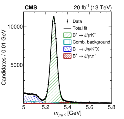
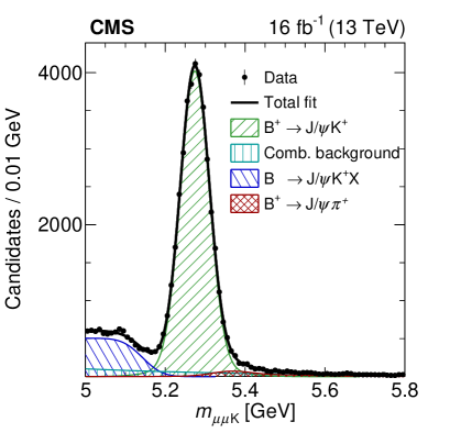
Figure 1: Invariant mass distributions for the $\mu\mu\PK$ system used to reconstruct the $\PBp\to\PJGy\PKp$ normalization sample. The plot on the left shows the 2016A central-region channel ($\abs{\eta^{\text{f}}_{\mu}}<0.7$), while the plot on the right shows the 2016B forward-region channel ($0.7<\abs{\eta^{\text{f}}_{\mu}}<1.4$). The mass resolutions for these channels are $30$ and $43\MeV$, respectively. The data are shown by solid black circles, the result of the fit is overlaid with the black line, and the different components are indicated by the hatched regions.

The $\PB$ candidate yields in the normalization sample are determined with binned ML fits. Example invariant mass distributions from Run 2 are shown in Fig. 1. The $\PBp\to\PJGy\PKp$ signal component is modeled by a double-Gaussian function with common mean. The background is modeled with an exponential function for the combinatorial component, an error function for the partially reconstructed background from $\PB\to\PJGy\PK X$, and a double-Gaussian function with common mean for $\PBp\to\PJGy\PGpp$ decays. For this latter component, the integral is constrained to 4% of the signal yield [16] and the other parameters are fixed to the expectation from MC simulation. The total $\PBp\to\PJGy\PKp$ yield used for the determination of $\mathcal{B}(\PBzs\to\MM)$ is $N_{\text{obs}}^{\PBp}=(1.43\pm 0.06)\times 10^{6}$, where the uncertainty combines the statistical and systematic components (see Table 0.7 below for the yields in different running periods and channels). The systematic uncertainty in the $\PBp\to\PJGy\PKp$ yield is approximately 4% and is determined by comparing the yields when fitting with or without a $\PJGy$ mass constraint.

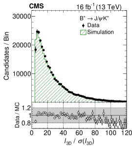
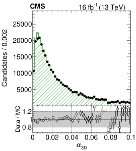
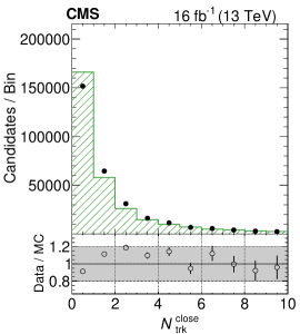
Figure 2: Comparison of measured and simulated $\PBp\to\PJGy\PKp$ distributions for the most discriminating analysis BDT variables in the central channel for 2016B: the flight length significance, the pointing angle, and the number of tracks close to the secondary vertex. The events are required to pass the preselection for the analysis BDT training. See text for details. The background-subtracted data are shown by solid circles and the MC simulation by the hatched histogram. The MC histograms are normalized to the number of events in the data. The lower panels display the ratio of the data to the MC simulation. The band in the ratio plot illustrates a $\pm 20\%$ variation.

Background-subtracted data distributions are compared to simulation for both the $\PBp\to\PJGy\PKp$ and $\PBzs\to\PJGy\PGf$ candidate event samples. As examples, Fig. 2 shows the most discriminating variables used in the analysis BDT: the flight length significance $\ell_{\mathrm{3D}}/\sigma(\ell_{\mathrm{3D}})$, the pointing angle $\alpha$, and the number of close tracks $N_{\text{trk}}^{\text{close}}$. The distributions are shown for the central channel in the 2016B data sample after the loose preselection for the analysis BDT training has been applied. The ratio between the background-subtracted data and the simulation is shown in the lower plots. The shaded bands in the ratio plots, included for illustration, demonstrate that the data-simulation difference can be as large as around 20%, mostly in peripheral parts of the distributions (the same comment applies to the analogous bands shown below in Figs. 3 and 4). These residual differences contribute to the systematic uncertainty in the analysis efficiency ratio between signal and normalization, where their impact is reduced. In Fig. 3, distributions of kinematic variables are displayed: the subleading muon , the cosine of the muon helicity angle $\theta_{\Pgmm}$ ($\theta_{\Pgmm}$ is the angle in the $\PJGy$ rest frame between the $\Pgmm$ and the $\PKp$ direction), and the meson candidate proper decay time. The $\PBp\to\PJGy\PKp$ analysis BDT discriminator distributions are plotted in Fig. 4. To illustrate the discrimination power of the analysis BDT, Fig. 4 also shows the BDT discriminator distributions from the $m_{\Pgmp\Pgmm}$ data sideband and the $\PBzs\to\MM$ signal MC simulation.

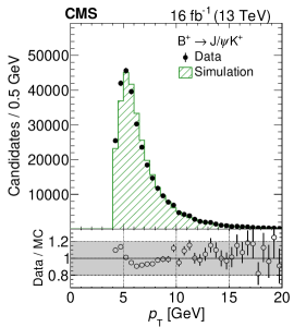
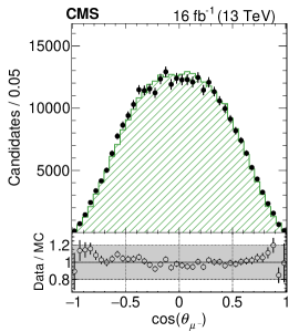
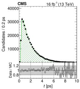
Figure 3: Comparison of measured and simulated $\PBp\to\PJGy\PKp$ distributions for kinematic variables in the central channel for 2016B: the subleading muon , the muon helicity angle, and the meson proper decay time. The events are required to pass the preselection for the analysis BDT training. See text for details. The background-subtracted data are shown by solid circles and the MC simulation by the hatched histogram. The MC histograms are normalized to the number of events in the data. The lower panels display the ratio of the data to the MC simulation. The band in the ratio plot illustrates a $\pm 20\%$ variation.

The systematic uncertainty in the analysis efficiency (accounting for losses in reconstruction, identification and selection) and in its ratio between the signal and normalization modes is estimated with the double ratio of analysis efficiencies between $\PBp\to\PJGy\PKp$ and $\PBzs\to\PJGy\PGf$ decays in data and MC simulation, based on the distributions in Fig. 4. The $\PBzs\to\PJGy\PGf$ control sample is used in this context as a placeholder for the signal because of the statistical limitations of the data signal events. Just as the normalization sample has one additional track compared to the signal sample, the control sample has one additional track compared to the normalization sample. Applying the analysis BDT discriminator requirements, the efficiency ratios are determined between the $\PBp\to\PJGy\PKp$ and $\PBzs\to\PJGy\PGf$  samples and subsequently the ratios between data and MC simulation are calculated for the double ratio. The deviation from unity is taken as the systematic uncertainty. In Run 2, it is approximately 5%, while in Run 1, it varies between 7 and 10% depending on the year and channel. For the effective lifetime determination, a small systematic uncertainty of 0.02psassociated with the selection efficiency is estimated from a variation of the analysis BDT requirement.

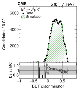
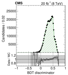
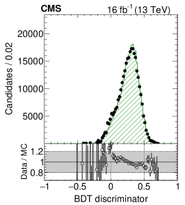
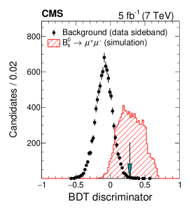
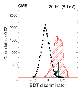
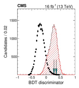
Figure 4: (Top row) Comparison of the analysis BDT discriminator distributions for $\PBp\to\PJGy\PKp$ in background-subtracted data and MC simulation in the central channel for 2011 (left column), 2012 (middle column), and 2016B (right column). The lower panels display the ratio of the data to the MC simulation. The band in the ratio plot illustrates a $\pm 20\%$ variation. (Bottom row) Illustration of the analysis BDT discriminator distribution in dimuon background data from the $5.45<m_{\Pgmp\Pgmm}<5.9\GeV$ sideband and $\PBzs\to\MM$ signal MC simulation. The distributions correspond to the full preselection and are normalized to the same number of entries. The solid markers show the data and the hatched histogram the MC simulation. The arrows show the BDT discriminator boundaries provided in Table 0.7.

The signal selection efficiency depends on the proper decay time because of selection requirements in the trigger and offline analysis. In the HLT, the increased instantaneous luminosity in Run 2 led to selection requirements on the maximum impact parameter of tracks relative to the interaction point. These requirements gradually reduce the efficiency for proper decay times larger than $6\unit{ps}$. The analysis selection requirements on isolation and on the separation of the candidate secondary vertex from the $\bbbar$-PV strongly reduce the efficiency for proper decay times below $1\unit{ps}$. The events in the signal MC simulation are reweighted to correspond to the SM expectation of $\tau_{\Pgmp\Pgmm}^{\text{SM}}=\tau_{{\PB}^{0}_{\mathrm{sH}}}=1.615\unit{ps}$ [16]. A priori, the effective lifetime is unknown, and we therefore use $\Delta\equiv[\varepsilon_{\text{tot}}(\tau_{{\PB}^{0}_{\mathrm{sH}}})-\varepsilon_{\text{tot}}(\tau_{{\PB}^{0}_{\mathrm{sL}}})]/\sqrt{12}$, where $\tau_{{\PB}^{0}_{\mathrm{sL}}}=1.415\unit{ps}$ [16], as the uncertainty associated with the effective lifetime uncertainty. It amounts to 1–3% in $\mathcal{B}(\PBzs\to\MM)$, depending on the channel and running period. For the  case, where the lifetime difference is much smaller, the average lifetime is used.

The systematic uncertainty due to differences between data and simulation for the production mechanism mixture is estimated as follows. In events with a $\PBp\to\PJGy\PKp$ or $\PBzs\to\PJGy\PGf$ candidate and a third muon $\mu_{3}$, presumed to originate from the decay of the other  hadron in the event, the variable $\Delta R(B,\mu_{3})$ provides discrimination between gluon splitting on the one hand and gluon fusion plus flavor excitation on the other. Templates from MC simulation are fit to the data distribution and used to determine the relative production mechanism fractions in data. Reweighting the fractions in the MC simulation to correspond to the fractions determined in data provides an estimate of 3% for the systematic uncertainty in the efficiency ratio.

To cross-check whether a significant variation in $f_{\PQs}/f_{\PQu}$ is observed with respect to the candidate kinematic variables $\eta$ (up to $\abs{\eta}<2.2$) and  (from 10 to 100), efficiency-corrected ratios of $\PBzs\to\PJGy\PGf$ and $\PBp\to\PJGy\PKp$ yields are studied. In addition, a sample of $\PBz\to\PJGy\PKst^{0}$ (with $\PK^{\ast 0}\to\PKp\Pgpm$) decays is reconstructed to perform the analogous cross-check for $f_{\PQs}/f_{\PQd}$, closely following the procedure discussed in Ref. [39]. No significant  or $\eta$ dependence is observed in either case.

A complementary approach for the study of the systematic uncertainty in the selection efficiency is to consider the standard deviation of the effective branching fraction $\mathcal{B}(\PBzs\to\PJGy\PGf)$ over all running periods and channels. For this purpose, the control sample yield is substituted for the signal yield in Eq. (3). The branching fraction $\mathcal{B}(\PBzs\to\PJGy\PGf)$ is affected by systematic uncertainties in the analysis BDT selection efficiency and yield determination, the kaon tracking efficiency, and possible differences between the isolation of  and  mesons due to their different fragmentation. A standard deviation of 4% is observed, substantially smaller than the combination of the above systematic uncertainty contributions. We conclude that the systematic uncertainties are not underestimated.

0.7 Branching fraction measurement

The branching fractions $\mathcal{B}(\PBzs\to\MM)$ and $\mathcal{B}(\PBz\to\MM)$ are determined with a 3D extended UML fit to the dimuon invariant mass $m_{\Pgmp\Pgmm}$ distribution, the relative mass resolution $\sigma(m_{\Pgmp\Pgmm})/m_{\Pgmp\Pgmm}$, and the binary distribution of the dimuon pairing configuration $\mathcal{C}$, where $\mathcal{C}=+1\ (-1)$ when the two muons bend towards (away from) each other in the magnetic field.

The fit model contains six components: the distributions of the signals $\PBzs\to\MM$ and $\PBz\to\MM$, the peaking background $\PB\to{\HepParticle{h}{}{}}{\HepParticle{h}{}{}}^{(\raisebox{-3.01389pt}{'})}$, the rare semileptonic background $\PB\to{\HepParticle{h}{}{}}\mu\nu$, the rare dimuon background $\PB\to{\HepParticle{h}{}{}}\mu\mu$, and the combinatorial background. The expected yields of the rare background components are normalized to the $\PBp\to\PJGy\PKp$ yield, corrected for the relative efficiency ratios and the respective production ratios. The PDF for each component $i$ (where $1\leq i\leq 6$) is

$$P_{i}(m_{\Pgmp\Pgmm},\sigma(m_{\Pgmp\Pgmm}),\mathcal{C})=P_{i}(m_{\Pgmp\Pgmm};\sigma(m_{\Pgmp\Pgmm}))\,P_{i}(\sigma(m_{\Pgmp\Pgmm})/m_{\Pgmp\Pgmm})\,P_{i}(\mathcal{C}),$$ (4)

where the $P_{i}$ terms are the PDFs for the indicated variable.

The binary $\mathcal{C}$ distribution is used in evaluating the possible underestimation of the $\PB\to{\HepParticle{h}{}{}}{\HepParticle{h}{}{}}^{(\raisebox{-3.01389pt}{'})}$ background. The misidentification probabilities for h and ${\HepParticle{h}{}{}}^{(\raisebox{-3.01389pt}{'})}$ are assumed to be independent. However, this assumption is not necessarily correct if the two tracks overlap in the detector. A possible residual enhancement of the double-hadron misidentification probability exists relative to the assumption that this probability factorizes into the product of two separately measured misidentification probabilities. Potential bias from this source can be reduced by requiring that both muon candidates satisfy very strict quality criteria or by demanding that the tracks be spatially separated. The effect is different for two muon candidates that bend towards or away from each other, and thus the $\mathcal{C}$  distribution is introduced. A scale factor is used in the fit to account for the change in the hadron misidentification rate if the hadron bends towards another muon candidate.

The signal PDFs are based on a Crystal Ball function [40] for the invariant mass and a nonparametric kernel estimator [41] with a superposition of Gaussian kernels for the relative mass resolution. The width $\sigma_{\text{CB}}$ of the Crystal Ball function is a conditional parameter with a linear dependence on the dimuon mass resolution $\sigma_{\text{CB}}=\kappa\,\sigma(m_{\Pgmp\Pgmm})$. All parameters, except for the normalizations, are fixed to values obtained from fits to the signal MC distributions. The dimuon mass scale is studied with $\PJGy\to\Pgmp\Pgmm$ and $\PgUa\to\Pgmp\Pgmm$ decays, interpolated to $m_{\PBzs}$. In Run 1, the MC PDF is shifted by $-6.0\ (-7.0)\MeV$ at the  mass for the central (forward) channel, while in Run 2 the shift is $-4.4\ (-3.1)\MeV$. The difference in the mass resolution between data and MC simulation is studied with $\PBp\to\PJGy\PKp$ events and is found to be 5%. Since correcting for this difference changes the measured branching fractions by only around 0.2%, no associated systematic uncertainty is assigned.

The peaking background is constructed from the sum of all $\PB\to{\HepParticle{h}{}{}}{\HepParticle{h}{}{}}^{(\raisebox{-3.01389pt}{'})}$ decay modes, weighted by the branching fraction, the product of the single-hadron misidentification probabilities, and the respective production ratios. We assume that the selection efficiency for the peaking background equals the signal selection efficiency. The trigger efficiency is taken as half the signal efficiency, with a 100% relative uncertainty because of the limited size of the MC event samples where both hadrons are misidentified as muons. The invariant mass PDF is modeled with the sum of a Gaussian and a Crystal Ball function with a common mean value. The relative mass resolution is modeled with a kernel estimator as for the signal PDF. The width of the mass distribution is independent of the per-candidate mass resolution and is fixed to the distribution obtained from the weighted sum of background sources in the MC simulation.

The shapes of the mass and relative mass resolution distributions for the rare semileptonic background are obtained by adding the MC expectations for $\Bz\to\Pgpm\Pgmp\nu$, $\PBzs\to\PKm\Pgmp\nu$, and $\PGLb\to\Pp\Pgmm\Pagngm$ decays, with a weighting as for the peaking background (with the exception of the trigger efficiency, which is taken to be equal to the signal efficiency). Both the mass and relative mass resolution distributions are modeled with kernel estimators. Rare dimuon background estimates are based on the decays $\Bz\to\Pgpz\Pgmp\Pgmm$ and $\PBm\to\Pgpm\Pgmp\Pgmm$, with the mass and relative mass resolution PDFs modeled with nonparametric kernel estimators. To account for missing contributions and efficiency differences with respect to the signal, these background components ($\PB\to{\HepParticle{h}{}{}}\mu\nu$ and $\PB\to{\HepParticle{h}{}{}}\mu\mu$) are scaled with a common factor such that their sum, when added to the combinatorial background, which is extrapolated from the sideband, matches the event yield of data events in the mass region $4.9<m_{\Pgmp\Pgmm}<5.2\GeV$.

The normalizations of all of the rare background components are constrained within the combined uncertainties of the branching fractions, misidentification probabilities, and efficiencies. For the peaking background, the combined relative uncertainty is about 100%, while the rare semileptonic and dimuonic background components have relative uncertainties of order 15%.

The combinatorial background invariant mass distribution is modeled by a nonnegative Bernstein polynomial of the first degree, whose parameters (both slope and normalization) are determined in the fit. The fit result changes by 2.3% (0.6%) for $\PBzs\to\MM$ ($\PBz\to\MM$) when using an exponential function instead. This is included as a systematic uncertainty. The relative mass resolution is modeled by a kernel function, determined from the events in the mass data sideband.

In the UML fit, the parameters of interest are $\mathcal{B}(\PBzs\to\MM)$ and $\mathcal{B}(\PBz\to\MM)$. The nuisance parameters are profiled, subject to constraints. Gaussian constraints are used for the uncertainties in $\mathcal{B}(\PBp\to\PJGy\PKp)$, the ratio of efficiencies $\varepsilon_{\text{tot}}^{\PBp}/\varepsilon_{\text{tot}}$, and the yields of the normalization sample. For the smaller yields of $\PB\to{\HepParticle{h}{}{}}\mu\nu$, $\PB\to{\HepParticle{h}{}{}}\mu\mu$, and $\PB\to{\HepParticle{h}{}{}}{\HepParticle{h}{}{}}^{(\raisebox{-3.01389pt}{'})}$ decays, log-normal priors are used as constraints. Prior to analyzing the events in the signal region, extensive tests were performed with pseudo-experiments to assess the sensitivity of the fitting procedure as well as its robustness and accuracy.

As mentioned in the Introduction, the data are divided into two channels (central or forward) depending on the pseudorapidity of the most forward muon $\abs{\eta^{\text{f}}_{\mu}}$, and into data collection running periods (2011, 2012, 2016A, and 2016B). The separation between the central and forward channels differs between Run 1 and Run 2 because of limitations imposed by the larger trigger rates in Run 2. In Run 1, the central (forward) channel covers $\abs{\eta^{\text{f}}_{\mu}}<1.4$ ($1.4<\abs{\eta^{\text{f}}_{\mu}}<2.1$) and in Run 2, $\abs{\eta^{\text{f}}_{\mu}}<0.7$ ($0.7<\abs{\eta^{\text{f}}_{\mu}}<1.4$). In total, there are eight channels: central and forward in four data-taking running periods. To maximize the sensitivity, channels with sufficient statistical precision are divided into mutually exclusive categories, a low- and a high-range category in the analysis BDT discriminator. The low-range category extends from the boundary given in the first row in Table 0.7 to the boundary in the second row. The high range extends from the boundary in the second row to $+1$. These analysis BDT discriminator requirements are determined by maximizing the expected sensitivity using the full UML fit framework. The boundaries differ between data-taking running periods because the distributions in the analysis BDT discriminator value differ. In summary, the UML fit is performed simultaneously in 14 categories.

Analysis BDT discriminator boundaries per category, channel, and running period for the branching fraction determination (2011 has only one category because of the small sample size). Examples of the requirements for the central channels are illustrated in Fig. 4 (bottom row). 2011 2012 2016A 2016B Central Forward Central Forward Central Forward Central Forward Low — — 0.27 0.23 0.19 0.19 0.18 0.23 High 0.28 0.21 0.35 0.32 0.30 0.30 0.31 0.38

Figure 5 (left) shows the mass distribution for the combined high-range analysis BDT categories, with the fit results overlaid. The $\PBzs\to\MM$ signal contribution is clearly visible. The corresponding distribution for the combined low-range BDT categories is shown in Fig. 5 (right). The result of the fit to the data in the 14 categories defined in Table 0.7 is

$$\mathcal{B}(\PBzs\to\MM)=[2.9\pm{0.7}\,(\text{exp})\pm{0.2}\,(\text{frag})]\times 10^{-9},$$ (5)

where the experimental uncertainty combines the dominant statistical and systematical terms. The second uncertainty is due to the uncertainty in $f_{\PQs}/f_{\PQu}$. The systematic uncertainties are summarized in Table 0.7. The event yields of the fit components, the average  of the $\PBzs\to\MM$ signal, and the efficiency ratios are given in Table 0.7. Summing over all categories, we observe a total $\PBzs\to\MM$ yield of $61\ ^{+15}_{-13}$ candidates. The observed (expected) significance, determined using Wilks’ theorem [42], is $5.6$ ($6.5$) standard deviations. The average $\pt$ of all $\PBzs\to\MM$ signal candidates is 17.2. The fit also provides the result $\mathcal{B}(\PBz\to\MM)=(0.8\,^{+1.4}_{-1.3})\times 10^{-10}$. The observed (expected) significance of this result is $0.6$ ($0.8$) standard deviations based on Wilks’ theorem, treating $\mathcal{B}(\PBzs\to\MM)$ as a nuisance parameter. With the Feldman-Cousins approach [43], an observed significance of $1.0$ standard deviation is obtained.

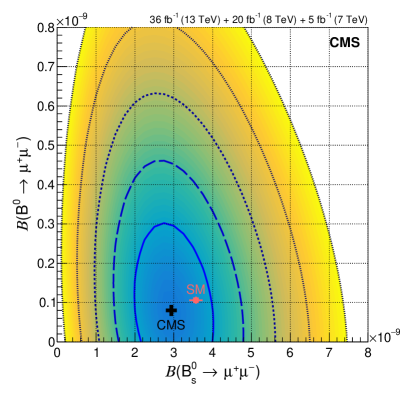
Figure 6: (Left) Likelihood contours for the fit to the branching fractions $\mathcal{B}(\PBzs\to\MM)$ and $\mathcal{B}(\PBz\to\MM)$, together with the best-fit value (cross) and the SM expectation (solid square). The contours correspond to regions with 1–5 standard deviation coverage. (Right) The quantity $1-\CL$ as a function of the assumed $\PBz\to\MM$ branching fraction. The dashed curve shows the median expected value for the background-only hypothesis, while the solid line is the observed value. The shaded region indicates the $\pm 1$ standard deviation uncertainty band.

The likelihood contours of the fit are shown in Fig. 6 (left), together with the SM expectation. The correlation coefficient between the two branching fractions is $-0.181$.

Since no significant signal is observed for $\PBz\to\MM$, one-sided upper limits are determined using the standard  rule [44, 45], with the LHC-type profiled likelihood as the test statistic. The result is $\mathcal{B}(\PBz\to\MM)<3.6\times 10^{-10}\ (3.1\times 10^{-10})$ at $95$ ($90$)% confidence level (). The corresponding expected upper limit, assuming no signal, is $\mathcal{B}(\PBz\to\MM)<3.0\times 10^{-10}\ (2.4\times 10^{-10})$. In Fig. 6 (right), the observed and expected confidence levels ($1-\CL$) are shown versus the assumed $\PBz\to\MM$ branching fraction. In interpreting Fig. 6 (right), it is important to remember that the background-only hypothesis does not include the $\PBz\to\MM$ signal expected in the SM.

All observed results are consistent within the uncertainties with the SM expectations. Restricting the present analysis to the Run 1 data results in an observed branching fraction of $\mathcal{B}(\PBzs\to\MM)=(2.3\ ^{+1.0}_{-0.8})\times 10^{-9}$ with an observed (expected) significance of $3.3$ ($4.5$) standard deviations. This is consistent with the results of Ref. [12] when that analysis is restricted to the CMS data set. The upper limit on $\mathcal{B}(\PBz\to\MM)$ is substantially improved compared to the limit of our previous study [11], even when using Run 1 data alone, because of more stringent muon identification criteria and the introduction of the UML fit.

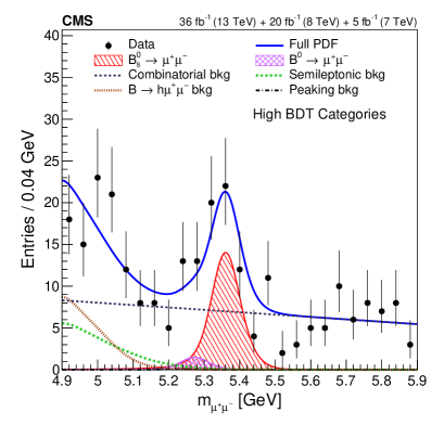
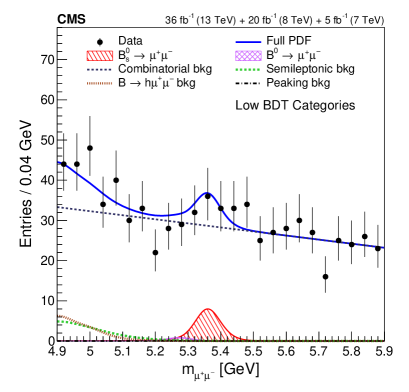
Figure 5: Invariant mass distributions with the fit projection overlays for the branching fraction results. The left (right) plot shows the combined results from the high- (low-)range analysis BDT categories defined in Table 0.7. The total fit is shown by the solid line and the different background components by the broken lines. The signal components are shown by the hatched distributions.

Summary of systematic uncertainty sources described in the text. The uncertainties quoted for the branching fraction $\mathcal{B}(\PBzs\to\MM)$ are relative uncertainties, while the uncertainties for the effective lifetime $\tau_{\Pgmp\Pgmm}$ are absolute and are given for both the 2D UML and sPlot analysis methods. The relative uncertainties in the upper limit on $\mathcal{B}(\PBz\to\MM)$ differ for the background yields and parametrization, but have negligible impact on that result. The bottom rows provide the total systematic uncertainty and the total uncertainty in the branching fraction and the effective lifetime measurements. Contributions that are included in other items are indicated by (*). Non-applicable sources are marked with dashes. Source $\mathcal{B}(\PBzs\to\MM)$ [%] $\tau_{\Pgmp\Pgmm}$ [ps] 2D UML sPlot Kaon tracking 2.3–4 — — Normalization yield 4 — — Background yields 1 0.03 (*) Production process 3 — — Muon identification 3 — — Trigger 3 — — Efficiency (data/MC simulation) 5–10 — (*) Efficiency (functional form) — 0.01 0.04 Efficiency lifetime dependence 1–3 (*) (*) Running period dependence 5–6 0.07 0.07 BDT discriminator threshold — 0.02 0.02 Silicon tracker alignment — 0.02 — Finite size of MC sample — 0.03 — Background parametrization/Fit bias 2.3 — 0.09 $\mathcal{C}$ correction — 0.01 0.01 Absolute total systematic uncertainty $0.3\times 10^{-9}$ 0.09 0.12 Absolute total uncertainty $0.7\times 10^{-9}$ ${}^{+0.61}_{-0.44}$ ${}^{+0.52}_{-0.33}$

Summary of the fitted yields for $\PBzs\to\MM$, $\PBz\to\MM$, the combinatorial background for $5.2<m_{\Pgmp\Pgmm}<5.45\GeV$, and the $\PBp\to\PJGy\PKp$ normalization, the average  of the $\PBzs\to\MM$ signal, and the ratio of efficiencies between the normalization and the signal for all 14 categories of the 3D UML branching fraction fit. The high and low ranges of the analysis BDT discriminator distribution are defined in Table 0.7. The size of the peaking background is 5–10% of the $\PBz\to\MM$ signal. The average  is calculated from the MC simulation and has negligible uncertainties. The uncertainties shown include the statistical and systematic components. It should be noted that the $\PBzs\to\MM$ and $\PBz\to\MM$ yields and their uncertainties are determined from the branching fraction fit and also include the normalization uncertainties. Category $N(\PBzs)$ $N(\Bz)$ $N_{\text{comb}}$ $N_{\text{obs}}^{\PBp}/100$ $\langle\pt(\PBzs)\rangle[\GeV]$ $\varepsilon_{\text{tot}}/\varepsilon_{\text{tot}}^{\PBp}$ 2011/central $3.6\ ^{+0.9}_{-0.8}$ $0.4\ ^{+0.7}_{-0.6}$ $2.3\pm 1.0$ $750\pm 30$ $16.4$ $3.9\pm 0.5$ 2011/forward $2.0\ ^{+0.5}_{-0.4}$ $0.2\ ^{+0.4}_{-0.3}$ $0.7\pm 0.5$ $220\pm 10$ $14.9$ $7.5\pm 0.8$ 2012/central/low $3.7\ ^{+0.9}_{-0.8}$ $0.4\ ^{+0.6}_{-0.6}$ $29.9\pm 2.9$ $790\pm 30$ $16.1$ $3.8\pm 0.5$ 2012/central/high $9.3\ ^{+2.3}_{-2.1}$ $1.0\ ^{+1.7}_{-1.6}$ $7.6\pm 1.8$ $2360\pm 100$ $17.3$ $3.2\pm 0.4$ 2012/forward/low $1.7\ ^{+0.4}_{-0.4}$ $0.2\ ^{+0.3}_{-0.3}$ $29.9\pm 2.9$ $190\pm 10$ $14.3$ $7.3\pm 1.0$ 2012/forward/high $4.7\ ^{+1.2}_{-1.1}$ $0.5\ ^{+0.9}_{-0.8}$ $8.3\pm 1.7$ $660\pm 30$ $15.5$ $5.9\pm 0.8$ 2016A/central/low $2.2\ ^{+0.5}_{-0.5}$ $0.2\ ^{+0.4}_{-0.4}$ $10.3\pm 1.7$ $580\pm 20$ $17.5$ $3.1\pm 0.4$ 2016A/central/high $4.0\ ^{+1.0}_{-0.9}$ $0.4\ ^{+0.8}_{-0.7}$ $3.4\pm 1.2$ $1290\pm 60$ $19.3$ $2.5\pm 0.3$ 2016A/forward/low $3.7\ ^{+0.9}_{-0.8}$ $0.4\ ^{+0.7}_{-0.7}$ $43.5\pm 3.5$ $780\pm 30$ $15.8$ $3.9\pm 0.5$ 2016A/forward/high $8.1\ ^{+2.0}_{-1.8}$ $0.8\ ^{+1.5}_{-1.4}$ $15.9\pm 2.4$ $1920\pm 80$ $17.5$ $3.4\pm 0.4$ 2016B/central/low $4.1\ ^{+1.0}_{-0.9}$ $0.4\ ^{+0.8}_{-0.7}$ $34.4\pm 3.2$ $1020\pm 40$ $17.2$ $3.3\pm 0.4$ 2016B/central/high $3.6\ ^{+0.9}_{-0.8}$ $0.4\ ^{+0.7}_{-0.6}$ $2.2\pm 1.0$ $1320\pm 50$ $20.8$ $2.2\pm 0.2$ 2016B/forward/low $6.1\ ^{+1.5}_{-1.4}$ $0.6\ ^{+1.1}_{-1.0}$ $33.4\pm 3.1$ $1260\pm 50$ $16.2$ $3.9\pm 0.4$ 2016B/forward/high $3.9\ ^{+1.0}_{-0.9}$ $0.4\ ^{+0.8}_{-0.7}$ $4.0\pm 1.3$ $1180\pm 50$ $19.5$ $2.7\pm 0.3$

0.8 Effective lifetime measurement

Two independent fitting methods were developed to determine the $\PBzs\to\MM$ effective lifetime, in order to allow for extensive validation, cross-checks, and systematic studies. The primary method consists of an extended 2D UML fit to the dimuon invariant mass and proper decay time [46, 39]. The second method employs a 1D approach in which the background is subtracted using the sPlot [23] technique, with a function then fitted to the background-subtracted distribution using a binned ML. The 2D UML approach was chosen as the primary method, prior to analyzing the events in the signal region, because it exhibited better median expected performance.

A slightly modified analysis BDT setup is used for both approaches. For simplicity, a single BDT discriminator requirement, as indicated in Table 0.8, is used for each channel. As before, these requirements are determined by optimizing the expected performance.

Analysis BDT discriminator minimum requirements per channel and running period for the 1D and 2D effective lifetime fits. 2011 2012 2016A 2016B Central Forward Central Forward Central Forward Central Forward 0.22 0.19 0.32 0.32 0.22 0.30 0.22 0.29

The fits are performed over the decay time range $1<t<11\unit{ps}$. For very short times, the reconstruction efficiency is small because of the flight-length significance and isolation requirements, while for long times, the efficiency is reduced in Run 2 because of the HLT requirements. The results of both approaches are limited by the small number of signal events. Systematic uncertainties have only a small impact on the total uncertainty.

0.8.1 Two-dimensional unbinned maximum likelihood fit

The extended 2D UML fit uses the proper decay time resolution, $\sigma_{t}$, as a conditional parameter. The unnormalized PDF $\mathcal{P}$ has the following expression:

$$\begin{split}\mathcal{P}(m_{\Pgmp\Pgmm},t;\sigma_{t})=N_{\text{sig}}P_{\text{sig}}(m_{\Pgmp\Pgmm})T_{\text{sig}}(t;\sigma_{t})\varepsilon_{\text{sig}}(t)+N_{\text{comb}}P_{\text{comb}}(m_{\Pgmp\Pgmm})T_{\text{comb}}(t;\sigma_{t})\\ +N_{\text{peak}}P_{\text{peak}}(m_{\Pgmp\Pgmm})T_{\text{peak}}(t;\sigma_{t})\varepsilon_{\text{peak}}(t)+N_{\text{semi}}P_{\text{semi}}(m_{\Pgmp\Pgmm})T_{\text{semi}}(t;\sigma_{t})\varepsilon_{\text{semi}}(t),\end{split}$$ (6)

where $N_{\text{sig}}$, $N_{\text{comb}}$, $N_{\text{peak}}$, and $N_{\text{semi}}$ are the $\PBzs\to\MM$ signal, combinatorial, peaking (both $\PBz\to\MM$ and $\PB\to{\HepParticle{h}{}{}}{\HepParticle{h}{}{}}^{(\raisebox{-3.01389pt}{'})}$), and semileptonic ($\PB\to{\HepParticle{h}{}{}}\mu\nu$ combined with $\PB\to{\HepParticle{h}{}{}}\mu\mu$) background yield Poisson terms, respectively. The invariant mass and decay time PDFs for the signal and background components are described by $P(m_{\Pgmp\Pgmm})$ and $T(t;\sigma_{t})$, respectively. The efficiencies $\varepsilon_{\text{sig}}$, $\varepsilon_{\text{peak}}$, and $\varepsilon_{\text{semi}}$ for the signal and background components as a function of the proper decay time are determined from simulated event samples.

For the PDFs describing the dimuon invariant mass distribution ($P_{\text{sig}},P_{\text{comb}},P_{\text{peak}},P_{\text{semi}}$), the signal shape is parametrized by a Crystal Ball function, while the combinatorial, peaking, and semileptonic background contributions are parametrized by a nonnegative Bernstein polynomial of the first degree, the sum of a Crystal Ball function and a Gaussian function with common mean, and a Gaussian function, respectively. For the PDFs describing the proper decay time distributions ($T_{\text{sig}},T_{\text{comb}},T_{\text{peak}},T_{\text{semi}}$), the signal and background shapes are parametrized by individual exponential functions, which are convolved with a Gaussian function to incorporate the effect of the detector resolution, and with the $T_{\text{sig}}$ exponential function depending on the effective lifetime. The signal, peaking, and semileptonic background proper decay time PDFs are corrected with their respective efficiency factors ($\varepsilon_{\text{sig}},\varepsilon_{\text{peak}},\varepsilon_{\text{semi}}$). Such a correction is not applied to the combinatorial background since the decay time PDF $T_{\text{comb}}$ is modeled from data directly. The modeling of the efficiency function has a systematic uncertainty of about $0.01\unit{ps}$, determined by variation of the parametrization.

The signal yield, the effective lifetime $\tau_{\Pgmp\Pgmm}$, and all parameters of the combinatorial background (except the combinatorial background in the forward channel of 2011, which is held fixed because there are no events in the sideband) are determined in the fit. All other parameters are either constrained (background yields of the peaking and semileptonic components inside log-normal constraints) or fixed to the MC simulation values (all other parameters). The UML fit is performed simultaneously in the eight independent channels defined in Table 0.8.

The combined mass and proper decay time distributions from all channels, with the fit results overlaid, are shown in Fig. 7. The effective lifetime obtained from the fit is

$$\tau_{\Pgmp\Pgmm}=1.70\,^{+0.61}_{-0.44}\unit{ps},$$ (7)

where the uncertainty represents the combined statistical and systematic terms. Systematic uncertainties, beyond those already discussed, include small contributions from the limited statistical precision of the MC simulation ($0.03\unit{ps}$) and the $\mathcal{C}$ correction ($0.01\unit{ps}$). All systematic uncertainties are summarized in Table 0.7.

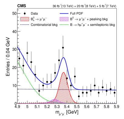
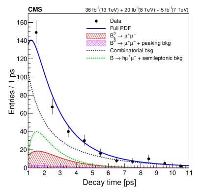
Figure 7: Invariant mass (left) and proper decay time (right) distributions, with the 2D UML fit projections overlaid. The data combine all channels passing the analysis BDT discriminator requirements as given in Table 0.8. The total fit is shown by the solid line and the different background components by the broken lines and cross-hatched distributions. The signal component is shown by the single-hatched distribution.

0.8.2 One-dimensional binned maximum likelihood fit

In the second method, the complete PDF described in Section 0.7 is used to determine sPlot weights. All events passing the analysis BDT requirements in Table 0.8, but without any proper decay time selection, are used for this step. Because of the small number of events in individual channels, an integration is performed over the central and forward channels for both the Run 1 and Run 2 data. The effective lifetime is determined with an exponential function modified to include the channel-dependent resolution and efficiency effects. To properly determine the uncertainty in the effective lifetime from the weighted fit, a custom algorithm [47] is implemented. This algorithm has several features. First, it performs a weighted binned ML fit to the sPlot distribution to provide the correct central value and covariance matrix. Second, to reduce biases associated with large histogram bin widths, it calculates the integral of the PDF, integrating over bins. Third, it incorporates a resolution and efficiency model into the effective decay time PDF. Finally, it provides asymmetric uncertainties in the fit parameters. The determined effective lifetime and the associated variance are consistent with the expectations from pseudo-experiments and the statistical uncertainties are in agreement with the confidence intervals reported by the Neyman construction [48].

Figure 8 shows the mass distribution of all contributing data, without requiring $t>1\unit{ps}$, and the weighted signal proper decay time distribution, together with the result of the binned ML fit. The fit yields $\tau_{\Pgmp\Pgmm}=1.55\ ^{+0.52}_{-0.33}\unit{ps}$, where the uncertainty is the combination of the statistical and systematic contributions. Using pseudo-experiments with post-fit nuisance parameters, a fit bias of $+0.09\unit{ps}$ is observed and corrected for in the result above. It is included as a systematic uncertainty. The reasons for this bias are, first, negative yields are not allowed in the weighted ML fit and, second, the sample size at large decay times is very small. The decay time dependence of the selection efficiency leads to a systematic uncertainty of $0.04\unit{ps}$. All systematic uncertainties are summarized in Table 0.7.

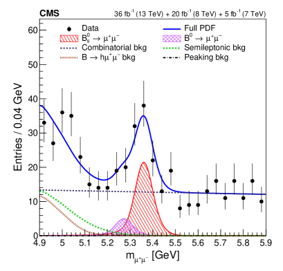
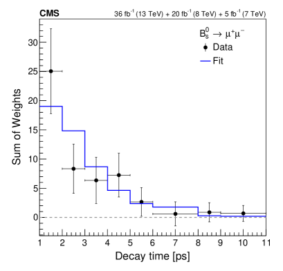
Figure 8: Invariant mass (left) and proper decay time (right) distributions, with the sPlot fit projections overlaid. The data combine all channels passing the analysis BDT discriminator requirements as given in Table 0.8. For the mass distribution, no requirement on the decay time is applied. The total fit is shown by the solid line, the different background components by the broken lines and cross-hatched distribution. The signal component is shown by the single-hatched distribution.

The two fitting methods, the 2D UML fit and the 1D sPlot approach, yield consistent results. The observed total uncertainties in the primary fitting method are about one root-mean-square deviation larger than the expected median uncertainties (${}^{+0.39}_{-0.30}\unit{ps}$). The expected median uncertainty for the 1D sPlot approach are ${}^{+0.49}_{-0.31}\unit{ps}$. While the uncertainties are sizable, the results are consistent with the SM expectation that only the heavy $\PB_{s\text{H}}$ state contributes to the $\PBzs\to\MM$ decay.

0.9 Summary

Measurements of the rare leptonic $\PB$ meson decays $\PBzs\to\MM$ and $\PBz\to\MM$ have been performed in $\Pp\Pp$ collision data collected by the CMS experiment at the LHC, corresponding to integrated luminosities of 5at center-of-mass energy 7, 20at 8, and 36at 13. The $\PBzs\to\MM$ decay is observed with a significance of $5.6$ standard deviations and the time-integrated branching fraction is measured to be $\mathcal{B}(\PBzs\to\MM)=[2.9\pm{0.6}\stat\pm{0.3}\syst\pm{0.2}\,(\text{frag})]\times 10^{-9}$, where the last uncertainty refers to the uncertainty in the ratio of the  and the  fragmentation functions. No significant $\PBz\to\MM$ signal is observed and an upper limit $\mathcal{B}(\PBz\to\MM)<3.6\times 10^{-10}$ is determined at $95$% confidence level. The $\PBzs\to\MM$ effective lifetime is found to be $\tau_{\Pgmp\Pgmm}=[1.70\,^{+0.60}_{-0.43}\stat\pm{0.09}\syst]\unit{ps}$. The results for the branching fractions supersede the previous results from CMS [11], which were based on the 7 and 8 data only. All of the results are in agreement with the standard model predictions.

.10 The CMS Collaboration

Yerevan Physics Institute, Yerevan, Armenia
A.M. Sirunyan${}^{\textrm{\textdagger}}$, A. Tumasyan Institut für Hochenergiephysik, Wien, Austria
W. Adam, F. Ambrogi, T. Bergauer, J. Brandstetter, M. Dragicevic, J. Erö, A. Escalante Del Valle, M. Flechl, R. Frühwirth1, M. Jeitler1, N. Krammer, I. Krätschmer, D. Liko, T. Madlener, I. Mikulec, N. Rad, J. Schieck1, R. Schöfbeck, M. Spanring, D. Spitzbart, W. Waltenberger, C.-E. Wulz1, M. Zarucki Institute for Nuclear Problems, Minsk, Belarus
V. Drugakov, V. Mossolov, J. Suarez Gonzalez Universiteit Antwerpen, Antwerpen, Belgium
M.R. Darwish, E.A. De Wolf, D. Di Croce, X. Janssen, A. Lelek, M. Pieters, H. Rejeb Sfar, H. Van Haevermaet, P. Van Mechelen, S. Van Putte, N. Van Remortel Vrije Universiteit Brussel, Brussel, Belgium
F. Blekman, E.S. Bols, S.S. Chhibra, J. D’Hondt, J. De Clercq, D. Lontkovskyi, S. Lowette, I. Marchesini, S. Moortgat, Q. Python, K. Skovpen, S. Tavernier, W. Van Doninck, P. Van Mulders Université Libre de Bruxelles, Bruxelles, Belgium
D. Beghin, B. Bilin, H. Brun, B. Clerbaux, G. De Lentdecker, H. Delannoy, B. Dorney, L. Favart, A. Grebenyuk, A.K. Kalsi, A. Popov, N. Postiau, E. Starling, L. Thomas, C. Vander Velde, P. Vanlaer, D. Vannerom Ghent University, Ghent, Belgium
T. Cornelis, D. Dobur, I. Khvastunov2, M. Niedziela, C. Roskas, M. Tytgat, W. Verbeke, B. Vermassen, M. Vit Université Catholique de Louvain, Louvain-la-Neuve, Belgium
O. Bondu, G. Bruno, C. Caputo, P. David, C. Delaere, M. Delcourt, A. Giammanco, V. Lemaitre, J. Prisciandaro, A. Saggio, M. Vidal Marono, P. Vischia, J. Zobec Centro Brasileiro de Pesquisas Fisicas, Rio de Janeiro, Brazil
F.L. Alves, G.A. Alves, G. Correia Silva, C. Hensel, A. Moraes, P. Rebello Teles Universidade do Estado do Rio de Janeiro, Rio de Janeiro, Brazil
E. Belchior Batista Das Chagas, W. Carvalho, J. Chinellato3, E. Coelho, E.M. Da Costa, G.G. Da Silveira4, D. De Jesus Damiao, C. De Oliveira Martins, S. Fonseca De Souza, L.M. Huertas Guativa, H. Malbouisson, J. Martins5, D. Matos Figueiredo, M. Medina Jaime6, M. Melo De Almeida, C. Mora Herrera, L. Mundim, H. Nogima, W.L. Prado Da Silva, L.J. Sanchez Rosas, A. Santoro, A. Sznajder, M. Thiel, E.J. Tonelli Manganote3, F. Torres Da Silva De Araujo, A. Vilela Pereira Universidade Estadual Paulista ^a, Universidade Federal do ABC ^b, São Paulo, Brazil
C.A. Bernardes^a, L. Calligaris^a, T.R. Fernandez Perez Tomei^a, E.M. Gregores^b, D.S. Lemos, P.G. Mercadante^b, S.F. Novaes^a, SandraS. Padula^a Institute for Nuclear Research and Nuclear Energy, Bulgarian Academy of Sciences, Sofia, Bulgaria
A. Aleksandrov, G. Antchev, R. Hadjiiska, P. Iaydjiev, M. Misheva, M. Rodozov, M. Shopova, G. Sultanov University of Sofia, Sofia, Bulgaria
M. Bonchev, A. Dimitrov, T. Ivanov, L. Litov, B. Pavlov, P. Petkov Beihang University, Beijing, China
W. Fang7, X. Gao7, L. Yuan Department of Physics, Tsinghua University, Beijing, China
M. Ahmad, Z. Hu, Y. Wang Institute of High Energy Physics, Beijing, China
G.M. Chen, H.S. Chen, M. Chen, C.H. Jiang, D. Leggat, H. Liao, Z. Liu, A. Spiezia, J. Tao, E. Yazgan, H. Zhang, S. Zhang8, J. Zhao State Key Laboratory of Nuclear Physics and Technology, Peking University, Beijing, China
A. Agapitos, Y. Ban, G. Chen, A. Levin, J. Li, L. Li, Q. Li, Y. Mao, S.J. Qian, D. Wang, Q. Wang Zhejiang University, Hangzhou, China
M. Xiao Universidad de Los Andes, Bogota, Colombia
C. Avila, A. Cabrera, C. Florez, C.F. González Hernández, M.A. Segura Delgado Universidad de Antioquia, Medellin, Colombia
J. Mejia Guisao, J.D. Ruiz Alvarez, C.A. Salazar González, N. Vanegas Arbelaez University of Split, Faculty of Electrical Engineering, Mechanical Engineering and Naval Architecture, Split, Croatia
D. Giljanović, N. Godinovic, D. Lelas, I. Puljak, T. Sculac University of Split, Faculty of Science, Split, Croatia
Z. Antunovic, M. Kovac Institute Rudjer Boskovic, Zagreb, Croatia
V. Brigljevic, D. Ferencek, K. Kadija, B. Mesic, M. Roguljic, A. Starodumov9, T. Susa University of Cyprus, Nicosia, Cyprus
M.W. Ather, A. Attikis, E. Erodotou, A. Ioannou, M. Kolosova, S. Konstantinou, G. Mavromanolakis, J. Mousa, C. Nicolaou, F. Ptochos, P.A. Razis, H. Rykaczewski, D. Tsiakkouri Charles University, Prague, Czech Republic
M. Finger10, M. Finger Jr.10, A. Kveton, J. Tomsa Escuela Politecnica Nacional, Quito, Ecuador
E. Ayala Universidad San Francisco de Quito, Quito, Ecuador
E. Carrera Jarrin Academy of Scientific Research and Technology of the Arab Republic of Egypt, Egyptian Network of High Energy Physics, Cairo, Egypt
Y. Assran11^,12, S. Elgammal12 National Institute of Chemical Physics and Biophysics, Tallinn, Estonia
S. Bhowmik, A. Carvalho Antunes De Oliveira, R.K. Dewanjee, K. Ehataht, M. Kadastik, M. Raidal, C. Veelken Department of Physics, University of Helsinki, Helsinki, Finland
P. Eerola, L. Forthomme, H. Kirschenmann, K. Osterberg, M. Voutilainen Helsinki Institute of Physics, Helsinki, Finland
F. Garcia, J. Havukainen, J.K. Heikkilä, V. Karimäki, M.S. Kim, R. Kinnunen, T. Lampén, K. Lassila-Perini, S. Laurila, S. Lehti, T. Lindén, P. Luukka, T. Mäenpää, H. Siikonen, E. Tuominen, J. Tuominiemi Lappeenranta University of Technology, Lappeenranta, Finland
T. Tuuva IRFU, CEA, Université Paris-Saclay, Gif-sur-Yvette, France
M. Besancon, F. Couderc, M. Dejardin, D. Denegri, B. Fabbro, J.L. Faure, F. Ferri, S. Ganjour, A. Givernaud, P. Gras, G. Hamel de Monchenault, P. Jarry, C. Leloup, B. Lenzi, E. Locci, J. Malcles, J. Rander, A. Rosowsky, M.Ö. Sahin, A. Savoy-Navarro13, M. Titov, G.B. Yu Laboratoire Leprince-Ringuet, CNRS/IN2P3, Ecole Polytechnique, Institut Polytechnique de Paris
S. Ahuja, C. Amendola, F. Beaudette, P. Busson, C. Charlot, B. Diab, G. Falmagne, R. Granier de Cassagnac, I. Kucher, A. Lobanov, C. Martin Perez, M. Nguyen, C. Ochando, P. Paganini, J. Rembser, R. Salerno, J.B. Sauvan, Y. Sirois, A. Zabi, A. Zghiche Université de Strasbourg, CNRS, IPHC UMR 7178, Strasbourg, France
J.-L. Agram14, J. Andrea, D. Bloch, G. Bourgatte, J.-M. Brom, E.C. Chabert, C. Collard, E. Conte14, J.-C. Fontaine14, D. Gelé, U. Goerlach, M. Jansová, A.-C. Le Bihan, N. Tonon, P. Van Hove Centre de Calcul de l’Institut National de Physique Nucleaire et de Physique des Particules, CNRS/IN2P3, Villeurbanne, France
S. Gadrat Université de Lyon, Université Claude Bernard Lyon 1, CNRS-IN2P3, Institut de Physique Nucléaire de Lyon, Villeurbanne, France
S. Beauceron, C. Bernet, G. Boudoul, C. Camen, A. Carle, N. Chanon, R. Chierici, D. Contardo, P. Depasse, H. El Mamouni, J. Fay, S. Gascon, M. Gouzevitch, B. Ille, Sa. Jain, F. Lagarde, I.B. Laktineh, H. Lattaud, A. Lesauvage, M. Lethuillier, L. Mirabito, S. Perries, V. Sordini, L. Torterotot, G. Touquet, M. Vander Donckt, S. Viret Georgian Technical University, Tbilisi, Georgia
T. Toriashvili15 Tbilisi State University, Tbilisi, Georgia
Z. Tsamalaidze10 RWTH Aachen University, I. Physikalisches Institut, Aachen, Germany
C. Autermann, L. Feld, M.K. Kiesel, K. Klein, M. Lipinski, D. Meuser, A. Pauls, M. Preuten, M.P. Rauch, J. Schulz, M. Teroerde, B. Wittmer RWTH Aachen University, III. Physikalisches Institut A, Aachen, Germany
M. Erdmann, B. Fischer, S. Ghosh, T. Hebbeker, K. Hoepfner, H. Keller, L. Mastrolorenzo, M. Merschmeyer, A. Meyer, P. Millet, G. Mocellin, S. Mondal, S. Mukherjee, D. Noll, A. Novak, T. Pook, A. Pozdnyakov, T. Quast, M. Radziej, Y. Rath, H. Reithler, J. Roemer, A. Schmidt, S.C. Schuler, A. Sharma, S. Wiedenbeck, S. Zaleski RWTH Aachen University, III. Physikalisches Institut B, Aachen, Germany
G. Flügge, W. Haj Ahmad16, O. Hlushchenko, T. Kress, T. Müller, A. Nowack, C. Pistone, O. Pooth, D. Roy, H. Sert, A. Stahl17 Deutsches Elektronen-Synchrotron, Hamburg, Germany
M. Aldaya Martin, P. Asmuss, I. Babounikau, H. Bakhshiansohi, K. Beernaert, O. Behnke, A. Bermúdez Martínez, D. Bertsche, A.A. Bin Anuar, K. Borras18, V. Botta, A. Campbell, A. Cardini, P. Connor, S. Consuegra Rodríguez, C. Contreras-Campana, V. Danilov, A. De Wit, M.M. Defranchis, C. Diez Pardos, D. Domínguez Damiani, G. Eckerlin, D. Eckstein, T. Eichhorn, A. Elwood, E. Eren, E. Gallo19, A. Geiser, A. Grohsjean, M. Guthoff, M. Haranko, A. Harb, A. Jafari, N.Z. Jomhari, H. Jung, A. Kasem18, M. Kasemann, H. Kaveh, J. Keaveney, C. Kleinwort, J. Knolle, D. Krücker, W. Lange, T. Lenz, J. Lidrych, K. Lipka, W. Lohmann20, R. Mankel, I.-A. Melzer-Pellmann, A.B. Meyer, M. Meyer, M. Missiroli, G. Mittag, J. Mnich, A. Mussgiller, V. Myronenko, D. Pérez Adán, S.K. Pflitsch, D. Pitzl, A. Raspereza, A. Saibel, M. Savitskyi, V. Scheurer, P. Schütze, C. Schwanenberger, R. Shevchenko, A. Singh, H. Tholen, O. Turkot, A. Vagnerini, M. Van De Klundert, R. Walsh, Y. Wen, K. Wichmann, C. Wissing, O. Zenaiev, R. Zlebcik University of Hamburg, Hamburg, Germany
R. Aggleton, S. Bein, L. Benato, A. Benecke, V. Blobel, T. Dreyer, A. Ebrahimi, F. Feindt, A. Fröhlich, C. Garbers, E. Garutti, D. Gonzalez, P. Gunnellini, J. Haller, A. Hinzmann, A. Karavdina, G. Kasieczka, R. Klanner, R. Kogler, N. Kovalchuk, S. Kurz, V. Kutzner, J. Lange, T. Lange, A. Malara, J. Multhaup, C.E.N. Niemeyer, A. Perieanu, A. Reimers, O. Rieger, C. Scharf, P. Schleper, S. Schumann, J. Schwandt, J. Sonneveld, H. Stadie, G. Steinbrück, F.M. Stober, B. Vormwald, I. Zoi Karlsruher Institut fuer Technologie, Karlsruhe, Germany
M. Akbiyik, C. Barth, M. Baselga, S. Baur, T. Berger, E. Butz, R. Caspart, T. Chwalek, W. De Boer, A. Dierlamm, K. El Morabit, N. Faltermann, M. Giffels, P. Goldenzweig, A. Gottmann, M.A. Harrendorf, F. Hartmann17, U. Husemann, S. Kudella, S. Mitra, M.U. Mozer, D. Müller, Th. Müller, M. Musich, A. Nürnberg, G. Quast, K. Rabbertz, M. Schröder, I. Shvetsov, H.J. Simonis, R. Ulrich, M. Wassmer, M. Weber, C. Wöhrmann, R. Wolf Institute of Nuclear and Particle Physics (INPP), NCSR Demokritos, Aghia Paraskevi, Greece
G. Anagnostou, P. Asenov, G. Daskalakis, T. Geralis, A. Kyriakis, D. Loukas, G. Paspalaki National and Kapodistrian University of Athens, Athens, Greece
M. Diamantopoulou, G. Karathanasis, P. Kontaxakis, A. Manousakis-katsikakis, A. Panagiotou, I. Papavergou, N. Saoulidou, A. Stakia, K. Theofilatos, K. Vellidis, E. Vourliotis National Technical University of Athens, Athens, Greece
G. Bakas, K. Kousouris, I. Papakrivopoulos, G. Tsipolitis University of Ioánnina, Ioánnina, Greece
I. Evangelou, C. Foudas, P. Gianneios, P. Katsoulis, P. Kokkas, S. Mallios, K. Manitara, N. Manthos, I. Papadopoulos, J. Strologas, F.A. Triantis, D. Tsitsonis MTA-ELTE Lendület CMS Particle and Nuclear Physics Group, Eötvös Loránd University, Budapest, Hungary
M. Bartók21, R. Chudasama, M. Csanad, P. Major, K. Mandal, A. Mehta, M.I. Nagy, G. Pasztor, O. Surányi, G.I. Veres Wigner Research Centre for Physics, Budapest, Hungary
G. Bencze, C. Hajdu, D. Horvath22, F. Sikler, T.Á. Vámi, V. Veszpremi, G. Vesztergombi${}^{\textrm{\textdagger}}$ Institute of Nuclear Research ATOMKI, Debrecen, Hungary
N. Beni, S. Czellar, J. Karancsi21, A. Makovec, J. Molnar, Z. Szillasi Institute of Physics, University of Debrecen, Debrecen, Hungary
P. Raics, D. Teyssier, Z.L. Trocsanyi, B. Ujvari Eszterhazy Karoly University, Karoly Robert Campus, Gyongyos, Hungary
T. Csorgo, W.J. Metzger, F. Nemes, T. Novak Indian Institute of Science (IISc), Bangalore, India
S. Choudhury, J.R. Komaragiri, P.C. Tiwari National Institute of Science Education and Research, HBNI, Bhubaneswar, India
S. Bahinipati24, C. Kar, G. Kole, P. Mal, V.K. Muraleedharan Nair Bindhu, A. Nayak25, D.K. Sahoo24, S.K. Swain Panjab University, Chandigarh, India
S. Bansal, S.B. Beri, V. Bhatnagar, S. Chauhan, R. Chawla, N. Dhingra, R. Gupta, A. Kaur, M. Kaur, S. Kaur, P. Kumari, M. Lohan, M. Meena, K. Sandeep, S. Sharma, J.B. Singh, A.K. Virdi, G. Walia University of Delhi, Delhi, India
A. Bhardwaj, B.C. Choudhary, R.B. Garg, M. Gola, S. Keshri, Ashok Kumar, M. Naimuddin, P. Priyanka, K. Ranjan, Aashaq Shah, R. Sharma Saha Institute of Nuclear Physics, HBNI, Kolkata, India
R. Bhardwaj26, M. Bharti26, R. Bhattacharya, S. Bhattacharya, U. Bhawandeep26, D. Bhowmik, S. Dutta, S. Ghosh, B. Gomber27, M. Maity28, K. Mondal, S. Nandan, A. Purohit, P.K. Rout, G. Saha, S. Sarkar, T. Sarkar28, M. Sharan, B. Singh26, S. Thakur26 Indian Institute of Technology Madras, Madras, India
P.K. Behera, P. Kalbhor, A. Muhammad, P.R. Pujahari, A. Sharma, A.K. Sikdar Bhabha Atomic Research Centre, Mumbai, India
D. Dutta, V. Jha, V. Kumar, D.K. Mishra, P.K. Netrakanti, L.M. Pant, P. Shukla Tata Institute of Fundamental Research-A, Mumbai, India
T. Aziz, M.A. Bhat, S. Dugad, G.B. Mohanty, N. Sur, RavindraKumar Verma Tata Institute of Fundamental Research-B, Mumbai, India
S. Banerjee, S. Bhattacharya, S. Chatterjee, P. Das, M. Guchait, S. Karmakar, S. Kumar, G. Majumder, K. Mazumdar, N. Sahoo, S. Sawant Indian Institute of Science Education and Research (IISER), Pune, India
S. Dube, V. Hegde, B. Kansal, A. Kapoor, K. Kothekar, S. Pandey, A. Rane, A. Rastogi, S. Sharma Institute for Research in Fundamental Sciences (IPM), Tehran, Iran
S. Chenarani29, E. Eskandari Tadavani, S.M. Etesami29, M. Khakzad, M. Mohammadi Najafabadi, M. Naseri, F. Rezaei Hosseinabadi University College Dublin, Dublin, Ireland
M. Felcini, M. Grunewald INFN Sezione di Bari ^a, Università di Bari ^b, Politecnico di Bari ^c, Bari, Italy
M. Abbrescia^a,b, R. Aly^a,b,30, C. Calabria^a,b, A. Colaleo^a, D. Creanza^a,c, L. Cristella^a,b, N. De Filippis^a,c, M. De Palma^a,b, A. Di Florio^a,b, W. Elmetenawee^a,b, L. Fiore^a, A. Gelmi^a,b, G. Iaselli^a,c, M. Ince^a,b, S. Lezki^a,b, G. Maggi^a,c, M. Maggi^a, G. Miniello^a,b, S. My^a,b, S. Nuzzo^a,b, A. Pompili^a,b, G. Pugliese^a,c, R. Radogna^a, A. Ranieri^a, G. Selvaggi^a,b, L. Silvestris^a, F.M. Simone^a,b, R. Venditti^a, P. Verwilligen^a INFN Sezione di Bologna ^a, Università di Bologna ^b, Bologna, Italy
G. Abbiendi^a, C. Battilana^a,b, D. Bonacorsi^a,b, L. Borgonovi^a,b, S. Braibant-Giacomelli^a,b, R. Campanini^a,b, P. Capiluppi^a,b, A. Castro^a,b, F.R. Cavallo^a, C. Ciocca^a, G. Codispoti^a,b, M. Cuffiani^a,b, G.M. Dallavalle^a, F. Fabbri^a, A. Fanfani^a,b, E. Fontanesi^a,b, P. Giacomelli^a, C. Grandi^a, L. Guiducci^a,b, F. Iemmi^a,b, S. Lo Meo^a,31, S. Marcellini^a, G. Masetti^a, F.L. Navarria^a,b, A. Perrotta^a, F. Primavera^a,b, A.M. Rossi^a,b, T. Rovelli^a,b, G.P. Siroli^a,b, N. Tosi^a INFN Sezione di Catania ^a, Università di Catania ^b, Catania, Italy
S. Albergo^a,b,32, S. Costa^a,b, A. Di Mattia^a, R. Potenza^a,b, A. Tricomi^a,b,32, C. Tuve^a,b INFN Sezione di Firenze ^a, Università di Firenze ^b, Firenze, Italy
G. Barbagli^a, A. Cassese, R. Ceccarelli, V. Ciulli^a,b, C. Civinini^a, R. D’Alessandro^a,b, E. Focardi^a,b, G. Latino^a,b, P. Lenzi^a,b, M. Meschini^a, S. Paoletti^a, G. Sguazzoni^a, L. Viliani^a INFN Laboratori Nazionali di Frascati, Frascati, Italy
L. Benussi, S. Bianco, D. Piccolo INFN Sezione di Genova ^a, Università di Genova ^b, Genova, Italy
M. Bozzo^a,b, F. Ferro^a, R. Mulargia^a,b, E. Robutti^a, S. Tosi^a,b INFN Sezione di Milano-Bicocca ^a, Università di Milano-Bicocca ^b, Milano, Italy
A. Benaglia^a, A. Beschi^a,b, F. Brivio^a,b, V. Ciriolo^a,b,17, S. Di Guida^a,b,17, M.E. Dinardo^a,b, P. Dini^a, S. Gennai^a, A. Ghezzi^a,b, P. Govoni^a,b, L. Guzzi^a,b, M. Malberti^a, S. Malvezzi^a, D. Menasce^a, F. Monti^a,b, L. Moroni^a, M. Paganoni^a,b, D. Pedrini^a, S. Ragazzi^a,b, T. Tabarelli de Fatis^a,b, D. Zuolo^a,b INFN Sezione di Napoli ^a, Università di Napoli ’Federico II’ ^b, Napoli, Italy, Università della Basilicata ^c, Potenza, Italy, Università G. Marconi ^d, Roma, Italy
S. Buontempo^a, N. Cavallo^a,c, A. De Iorio^a,b, A. Di Crescenzo^a,b, F. Fabozzi^a,c, F. Fienga^a, G. Galati^a, A.O.M. Iorio^a,b, L. Lista^a,b, S. Meola^a,d,17, P. Paolucci^a,17, B. Rossi^a, C. Sciacca^a,b, E. Voevodina^a,b INFN Sezione di Padova ^a, Università di Padova ^b, Padova, Italy, Università di Trento ^c, Trento, Italy
P. Azzi^a, N. Bacchetta^a, D. Bisello^a,b, A. Boletti^a,b, A. Bragagnolo^a,b, R. Carlin^a,b, P. Checchia^a, P. De Castro Manzano^a, T. Dorigo^a, U. Dosselli^a, F. Gasparini^a,b, U. Gasparini^a,b, S.Y. Hoh^a,b, S. Lacaprara^a, P. Lujan^a, M. Margoni^a,b, A.T. Meneguzzo^a,b, J. Pazzini^a,b, M. Presilla^b, P. Ronchese^a,b, R. Rossin^a,b, F. Simonetto^a,b, A. Tiko^a, M. Tosi^a,b, M. Zanetti^a,b, P. Zotto^a,b, G. Zumerle^a,b INFN Sezione di Pavia ^a, Università di Pavia ^b, Pavia, Italy
A. Braghieri^a, D. Fiorina^a,b, P. Montagna^a,b, S.P. Ratti^a,b, V. Re^a, M. Ressegotti^a,b, C. Riccardi^a,b, P. Salvini^a, I. Vai^a, P. Vitulo^a,b INFN Sezione di Perugia ^a, Università di Perugia ^b, Perugia, Italy
M. Biasini^a,b, G.M. Bilei^a, D. Ciangottini^a,b, L. Fanò^a,b, P. Lariccia^a,b, R. Leonardi^a,b, E. Manoni^a, G. Mantovani^a,b, V. Mariani^a,b, M. Menichelli^a, A. Rossi^a,b, A. Santocchia^a,b, D. Spiga^a INFN Sezione di Pisa ^a, Università di Pisa ^b, Scuola Normale Superiore di Pisa ^c, Pisa, Italy
K. Androsov^a, P. Azzurri^a, G. Bagliesi^a, V. Bertacchi^a,c, L. Bianchini^a, T. Boccali^a, R. Castaldi^a, M.A. Ciocci^a,b, R. Dell’Orso^a, S. Donato^a, G. Fedi^a, L. Giannini^a,c, A. Giassi^a, M.T. Grippo^a, F. Ligabue^a,c, E. Manca^a,c, G. Mandorli^a,c, A. Messineo^a,b, F. Palla^a, A. Rizzi^a,b, G. Rolandi33, S. Roy Chowdhury, A. Scribano^a, P. Spagnolo^a, R. Tenchini^a, G. Tonelli^a,b, N. Turini, A. Venturi^a, P.G. Verdini^a INFN Sezione di Roma ^a, Sapienza Università di Roma ^b, Rome, Italy
F. Cavallari^a, M. Cipriani^a,b, D. Del Re^a,b, E. Di Marco^a,b, M. Diemoz^a, E. Longo^a,b, P. Meridiani^a, G. Organtini^a,b, F. Pandolfi^a, R. Paramatti^a,b, C. Quaranta^a,b, S. Rahatlou^a,b, C. Rovelli^a, F. Santanastasio^a,b, L. Soffi^a,b INFN Sezione di Torino ^a, Università di Torino ^b, Torino, Italy, Università del Piemonte Orientale ^c, Novara, Italy
N. Amapane^a,b, R. Arcidiacono^a,c, S. Argiro^a,b, M. Arneodo^a,c, N. Bartosik^a, R. Bellan^a,b, A. Bellora, C. Biino^a, A. Cappati^a,b, N. Cartiglia^a, S. Cometti^a, M. Costa^a,b, R. Covarelli^a,b, N. Demaria^a, B. Kiani^a,b, F. Legger, C. Mariotti^a, S. Maselli^a, E. Migliore^a,b, V. Monaco^a,b, E. Monteil^a,b, M. Monteno^a, M.M. Obertino^a,b, G. Ortona^a,b, L. Pacher^a,b, N. Pastrone^a, M. Pelliccioni^a, G.L. Pinna Angioni^a,b, A. Romero^a,b, M. Ruspa^a,c, R. Salvatico^a,b, V. Sola^a, A. Solano^a,b, D. Soldi^a,b, A. Staiano^a, D. Trocino^a,b INFN Sezione di Trieste ^a, Università di Trieste ^b, Trieste, Italy
S. Belforte^a, V. Candelise^a,b, M. Casarsa^a, F. Cossutti^a, A. Da Rold^a,b, G. Della Ricca^a,b, F. Vazzoler^a,b, A. Zanetti^a Kyungpook National University, Daegu, Korea
B. Kim, D.H. Kim, G.N. Kim, J. Lee, S.W. Lee, C.S. Moon, Y.D. Oh, S.I. Pak, S. Sekmen, D.C. Son, Y.C. Yang Chonnam National University, Institute for Universe and Elementary Particles, Kwangju, Korea
H. Kim, D.H. Moon, G. Oh Hanyang University, Seoul, Korea
B. Francois, T.J. Kim, J. Park Korea University, Seoul, Korea
S. Cho, S. Choi, Y. Go, S. Ha, B. Hong, K. Lee, K.S. Lee, J. Lim, J. Park, S.K. Park, Y. Roh, J. Yoo Kyung Hee University, Department of Physics
J. Goh Sejong University, Seoul, Korea
H.S. Kim Seoul National University, Seoul, Korea
J. Almond, J.H. Bhyun, J. Choi, S. Jeon, J. Kim, J.S. Kim, H. Lee, K. Lee, S. Lee, K. Nam, M. Oh, S.B. Oh, B.C. Radburn-Smith, U.K. Yang, H.D. Yoo, I. Yoon University of Seoul, Seoul, Korea
D. Jeon, H. Kim, J.H. Kim, J.S.H. Lee, I.C. Park, I.J Watson Sungkyunkwan University, Suwon, Korea
Y. Choi, C. Hwang, Y. Jeong, J. Lee, Y. Lee, I. Yu Riga Technical University, Riga, Latvia
V. Veckalns34 Vilnius University, Vilnius, Lithuania
V. Dudenas, A. Juodagalvis, A. Rinkevicius, G. Tamulaitis, J. Vaitkus National Centre for Particle Physics, Universiti Malaya, Kuala Lumpur, Malaysia
Z.A. Ibrahim, F. Mohamad Idris35, W.A.T. Wan Abdullah, M.N. Yusli, Z. Zolkapli Universidad de Sonora (UNISON), Hermosillo, Mexico
J.F. Benitez, A. Castaneda Hernandez, J.A. Murillo Quijada, L. Valencia Palomo Centro de Investigacion y de Estudios Avanzados del IPN, Mexico City, Mexico
H. Castilla-Valdez, E. De La Cruz-Burelo, I. Heredia-De La Cruz36, R. Lopez-Fernandez, A. Sanchez-Hernandez Universidad Iberoamericana, Mexico City, Mexico
S. Carrillo Moreno, C. Oropeza Barrera, M. Ramirez-Garcia, F. Vazquez Valencia Benemerita Universidad Autonoma de Puebla, Puebla, Mexico
J. Eysermans, I. Pedraza, H.A. Salazar Ibarguen, C. Uribe Estrada Universidad Autónoma de San Luis Potosí, San Luis Potosí, Mexico
A. Morelos Pineda University of Montenegro, Podgorica, Montenegro
J. Mijuskovic2, N. Raicevic University of Auckland, Auckland, New Zealand
D. Krofcheck University of Canterbury, Christchurch, New Zealand
S. Bheesette, P.H. Butler National Centre for Physics, Quaid-I-Azam University, Islamabad, Pakistan
A. Ahmad, M. Ahmad, Q. Hassan, H.R. Hoorani, W.A. Khan, M.A. Shah, M. Shoaib, M. Waqas AGH University of Science and Technology Faculty of Computer Science, Electronics and Telecommunications, Krakow, Poland
V. Avati, L. Grzanka, M. Malawski National Centre for Nuclear Research, Swierk, Poland
H. Bialkowska, M. Bluj, B. Boimska, M. Górski, M. Kazana, M. Szleper, P. Zalewski Institute of Experimental Physics, Faculty of Physics, University of Warsaw, Warsaw, Poland
K. Bunkowski, A. Byszuk37, K. Doroba, A. Kalinowski, M. Konecki, J. Krolikowski, M. Misiura, M. Olszewski, M. Walczak Laboratório de Instrumentação e Física Experimental de Partículas, Lisboa, Portugal
M. Araujo, P. Bargassa, D. Bastos, A. Di Francesco, P. Faccioli, B. Galinhas, M. Gallinaro, J. Hollar, N. Leonardo, T. Niknejad, J. Seixas, K. Shchelina, G. Strong, O. Toldaiev, J. Varela Joint Institute for Nuclear Research, Dubna, Russia
S. Afanasiev, P. Bunin, M. Gavrilenko, I. Golutvin, I. Gorbunov, A. Kamenev, V. Karjavine, A. Lanev, A. Malakhov, V. Matveev38^,39, P. Moisenz, V. Palichik, V. Perelygin, M. Savina, S. Shmatov, S. Shulha, N. Skatchkov, V. Smirnov, N. Voytishin, A. Zarubin Petersburg Nuclear Physics Institute, Gatchina (St. Petersburg), Russia
L. Chtchipounov, V. Golovtcov, Y. Ivanov, V. Kim40, E. Kuznetsova41, P. Levchenko, V. Murzin, V. Oreshkin, I. Smirnov, D. Sosnov, V. Sulimov, L. Uvarov, A. Vorobyev Institute for Nuclear Research, Moscow, Russia
Yu. Andreev, A. Dermenev, S. Gninenko, N. Golubev, A. Karneyeu, M. Kirsanov, N. Krasnikov, A. Pashenkov, D. Tlisov, A. Toropin Institute for Theoretical and Experimental Physics named by A.I. Alikhanov of NRC ‘Kurchatov Institute’, Moscow, Russia
V. Epshteyn, V. Gavrilov, N. Lychkovskaya, A. Nikitenko42, V. Popov, I. Pozdnyakov, G. Safronov, A. Spiridonov, A. Stepennov, M. Toms, E. Vlasov, A. Zhokin Moscow Institute of Physics and Technology, Moscow, Russia
T. Aushev National Research Nuclear University ’Moscow Engineering Physics Institute’ (MEPhI), Moscow, Russia
O. Bychkova, R. Chistov43, M. Danilov43, S. Polikarpov43, E. Tarkovskii P.N. Lebedev Physical Institute, Moscow, Russia
V. Andreev, M. Azarkin, I. Dremin, M. Kirakosyan, A. Terkulov Skobeltsyn Institute of Nuclear Physics, Lomonosov Moscow State University, Moscow, Russia
A. Belyaev, E. Boos, M. Dubinin44, L. Dudko, A. Ershov, A. Gribushin, V. Klyukhin, O. Kodolova, I. Lokhtin, S. Obraztsov, S. Petrushanko, V. Savrin, A. Snigirev Novosibirsk State University (NSU), Novosibirsk, Russia
A. Barnyakov45, V. Blinov45, T. Dimova45, L. Kardapoltsev45, Y. Skovpen45 Institute for High Energy Physics of National Research Centre ‘Kurchatov Institute’, Protvino, Russia
I. Azhgirey, I. Bayshev, S. Bitioukov, V. Kachanov, D. Konstantinov, P. Mandrik, V. Petrov, R. Ryutin, S. Slabospitskii, A. Sobol, S. Troshin, N. Tyurin, A. Uzunian, A. Volkov National Research Tomsk Polytechnic University, Tomsk, Russia
A. Babaev, A. Iuzhakov, V. Okhotnikov Tomsk State University, Tomsk, Russia
V. Borchsh, V. Ivanchenko, E. Tcherniaev University of Belgrade: Faculty of Physics and VINCA Institute of Nuclear Sciences
P. Adzic46, P. Cirkovic, M. Dordevic, P. Milenovic, J. Milosevic, M. Stojanovic Centro de Investigaciones Energéticas Medioambientales y Tecnológicas (CIEMAT), Madrid, Spain
M. Aguilar-Benitez, J. Alcaraz Maestre, A. Álvarez Fernández, I. Bachiller, M. Barrio Luna, CristinaF. Bedoya, J.A. Brochero Cifuentes, C.A. Carrillo Montoya, M. Cepeda, M. Cerrada, N. Colino, B. De La Cruz, A. Delgado Peris, J.P. Fernández Ramos, J. Flix, M.C. Fouz, O. Gonzalez Lopez, S. Goy Lopez, J.M. Hernandez, M.I. Josa, D. Moran, Á. Navarro Tobar, A. Pérez-Calero Yzquierdo, J. Puerta Pelayo, I. Redondo, L. Romero, S. Sánchez Navas, M.S. Soares, A. Triossi, C. Willmott Universidad Autónoma de Madrid, Madrid, Spain
C. Albajar, J.F. de Trocóniz, R. Reyes-Almanza Universidad de Oviedo, Instituto Universitario de Ciencias y Tecnologías Espaciales de Asturias (ICTEA), Oviedo, Spain
B. Alvarez Gonzalez, J. Cuevas, C. Erice, J. Fernandez Menendez, S. Folgueras, I. Gonzalez Caballero, J.R. González Fernández, E. Palencia Cortezon, V. Rodríguez Bouza, S. Sanchez Cruz Instituto de Física de Cantabria (IFCA), CSIC-Universidad de Cantabria, Santander, Spain
I.J. Cabrillo, A. Calderon, B. Chazin Quero, J. Duarte Campderros, M. Fernandez, P.J. Fernández Manteca, A. García Alonso, G. Gomez, C. Martinez Rivero, P. Martinez Ruiz del Arbol, F. Matorras, J. Piedra Gomez, C. Prieels, T. Rodrigo, A. Ruiz-Jimeno, L. Russo47, L. Scodellaro, I. Vila, J.M. Vizan Garcia University of Colombo, Colombo, Sri Lanka
K. Malagalage University of Ruhuna, Department of Physics, Matara, Sri Lanka
W.G.D. Dharmaratna, N. Wickramage CERN, European Organization for Nuclear Research, Geneva, Switzerland
D. Abbaneo, B. Akgun, E. Auffray, G. Auzinger, J. Baechler, P. Baillon, A.H. Ball, D. Barney, J. Bendavid, M. Bianco, A. Bocci, P. Bortignon, E. Bossini, C. Botta, E. Brondolin, T. Camporesi, A. Caratelli, G. Cerminara, E. Chapon, G. Cucciati, D. d’Enterria, A. Dabrowski, N. Daci, V. Daponte, A. David, O. Davignon, A. De Roeck, M. Deile, M. Dobson, M. Dünser, N. Dupont, A. Elliott-Peisert, N. Emriskova, F. Fallavollita48, D. Fasanella, S. Fiorendi, G. Franzoni, J. Fulcher, W. Funk, S. Giani, D. Gigi, A. Gilbert, K. Gill, F. Glege, L. Gouskos, M. Gruchala, M. Guilbaud, D. Gulhan, J. Hegeman, C. Heidegger, Y. Iiyama, V. Innocente, T. James, P. Janot, O. Karacheban20, J. Kaspar, J. Kieseler, M. Krammer1, N. Kratochwil, C. Lange, P. Lecoq, C. Lourenço, L. Malgeri, M. Mannelli, A. Massironi, F. Meijers, J.A. Merlin, S. Mersi, E. Meschi, F. Moortgat, M. Mulders, J. Ngadiuba, J. Niedziela, S. Nourbakhsh, S. Orfanelli, L. Orsini, F. Pantaleo17, L. Pape, E. Perez, M. Peruzzi, A. Petrilli, G. Petrucciani, A. Pfeiffer, M. Pierini, F.M. Pitters, D. Rabady, A. Racz, M. Rieger, M. Rovere, H. Sakulin, C. Schäfer, C. Schwick, M. Selvaggi, A. Sharma, P. Silva, W. Snoeys, P. Sphicas49, J. Steggemann, S. Summers, V.R. Tavolaro, D. Treille, A. Tsirou, G.P. Van Onsem, A. Vartak, M. Verzetti, W.D. Zeuner Paul Scherrer Institut, Villigen, Switzerland
L. Caminada50, K. Deiters, W. Erdmann, R. Horisberger, Q. Ingram, H.C. Kaestli, D. Kotlinski, U. Langenegger, T. Rohe, S.A. Wiederkehr ETH Zurich - Institute for Particle Physics and Astrophysics (IPA), Zurich, Switzerland
M. Backhaus, P. Berger, N. Chernyavskaya, G. Dissertori, M. Dittmar, M. Donegà, C. Dorfer, T.A. Gómez Espinosa, C. Grab, D. Hits, W. Lustermann, R.A. Manzoni, M.T. Meinhard, F. Micheli, P. Musella, F. Nessi-Tedaldi, F. Pauss, G. Perrin, L. Perrozzi, S. Pigazzini, M.G. Ratti, M. Reichmann, C. Reissel, T. Reitenspiess, B. Ristic, D. Ruini, D.A. Sanz Becerra, M. Schönenberger, L. Shchutska, M.L. Vesterbacka Olsson, R. Wallny, D.H. Zhu Universität Zürich, Zurich, Switzerland
T.K. Aarrestad, C. Amsler51, D. Brzhechko, M.F. Canelli, A. De Cosa, R. Del Burgo, B. Kilminster, S. Leontsinis, V.M. Mikuni, I. Neutelings, G. Rauco, P. Robmann, K. Schweiger, C. Seitz, Y. Takahashi, S. Wertz, A. Zucchetta National Central University, Chung-Li, Taiwan
T.H. Doan, C.M. Kuo, W. Lin, A. Roy, S.S. Yu National Taiwan University (NTU), Taipei, Taiwan
P. Chang, Y. Chao, K.F. Chen, P.H. Chen, W.-S. Hou, Y.y. Li, R.-S. Lu, E. Paganis, A. Psallidas, A. Steen Chulalongkorn University, Faculty of Science, Department of Physics, Bangkok, Thailand
B. Asavapibhop, C. Asawatangtrakuldee, N. Srimanobhas, N. Suwonjandee Çukurova University, Physics Department, Science and Art Faculty, Adana, Turkey
A. Bat, F. Boran, A. Celik52, S. Cerci53, S. Damarseckin54, Z.S. Demiroglu, F. Dolek, C. Dozen55, I. Dumanoglu, G. Gokbulut, EmineGurpinar Guler56, Y. Guler, I. Hos57, C. Isik, E.E. Kangal58, O. Kara, A. Kayis Topaksu, U. Kiminsu, G. Onengut, K. Ozdemir59, S. Ozturk60, A.E. Simsek, D. Sunar Cerci53, U.G. Tok, S. Turkcapar, I.S. Zorbakir, C. Zorbilmez Middle East Technical University, Physics Department, Ankara, Turkey
B. Isildak61, G. Karapinar62, M. Yalvac Bogazici University, Istanbul, Turkey
I.O. Atakisi, E. Gülmez, M. Kaya63, O. Kaya64, Ö. Özçelik, S. Tekten, E.A. Yetkin65 Istanbul Technical University, Istanbul, Turkey
A. Cakir, K. Cankocak, Y. Komurcu, S. Sen66 Istanbul University, Istanbul, Turkey
B. Kaynak, S. Ozkorucuklu Institute for Scintillation Materials of National Academy of Science of Ukraine, Kharkov, Ukraine
B. Grynyov National Scientific Center, Kharkov Institute of Physics and Technology, Kharkov, Ukraine
L. Levchuk University of Bristol, Bristol, United Kingdom
E. Bhal, S. Bologna, J.J. Brooke, D. Burns67, E. Clement, D. Cussans, H. Flacher, J. Goldstein, G.P. Heath, H.F. Heath, L. Kreczko, B. Krikler, S. Paramesvaran, B. Penning, T. Sakuma, S. Seif El Nasr-Storey, V.J. Smith, J. Taylor, A. Titterton Rutherford Appleton Laboratory, Didcot, United Kingdom
K.W. Bell, A. Belyaev68, C. Brew, R.M. Brown, D.J.A. Cockerill, J.A. Coughlan, K. Harder, S. Harper, J. Linacre, K. Manolopoulos, D.M. Newbold, E. Olaiya, D. Petyt, T. Reis, T. Schuh, C.H. Shepherd-Themistocleous, A. Thea, I.R. Tomalin, T. Williams, W.J. Womersley Imperial College, London, United Kingdom
R. Bainbridge, P. Bloch, J. Borg, S. Breeze, O. Buchmuller, A. Bundock, GurpreetSingh CHAHAL69, D. Colling, P. Dauncey, G. Davies, M. Della Negra, R. Di Maria, P. Everaerts, G. Hall, G. Iles, M. Komm, C. Laner, L. Lyons, A.-M. Magnan, S. Malik, A. Martelli, V. Milosevic, A. Morton, J. Nash70, V. Palladino, M. Pesaresi, D.M. Raymond, A. Richards, A. Rose, E. Scott, C. Seez, A. Shtipliyski, M. Stoye, T. Strebler, A. Tapper, K. Uchida, T. Virdee17, N. Wardle, D. Winterbottom, J. Wright, A.G. Zecchinelli, S.C. Zenz Brunel University, Uxbridge, United Kingdom
J.E. Cole, P.R. Hobson, A. Khan, P. Kyberd, C.K. Mackay, I.D. Reid, L. Teodorescu, S. Zahid Baylor University, Waco, USA
K. Call, B. Caraway, J. Dittmann, K. Hatakeyama, C. Madrid, B. McMaster, N. Pastika, C. Smith Catholic University of America, Washington, DC, USA
R. Bartek, A. Dominguez, R. Uniyal, A.M. Vargas Hernandez The University of Alabama, Tuscaloosa, USA
A. Buccilli, S.I. Cooper, C. Henderson, P. Rumerio, C. West Boston University, Boston, USA
A. Albert, D. Arcaro, Z. Demiragli, D. Gastler, C. Richardson, J. Rohlf, D. Sperka, I. Suarez, L. Sulak, D. Zou Brown University, Providence, USA
G. Benelli, B. Burkle, X. Coubez18, D. Cutts, Y.t. Duh, M. Hadley, U. Heintz, J.M. Hogan71, K.H.M. Kwok, E. Laird, G. Landsberg, K.T. Lau, J. Lee, Z. Mao, M. Narain, S. Sagir72, R. Syarif, E. Usai, D. Yu, W. Zhang University of California, Davis, Davis, USA
R. Band, C. Brainerd, R. Breedon, M. Calderon De La Barca Sanchez, M. Chertok, J. Conway, R. Conway, P.T. Cox, R. Erbacher, C. Flores, G. Funk, F. Jensen, W. Ko, O. Kukral, R. Lander, M. Mulhearn, D. Pellett, J. Pilot, M. Shi, D. Taylor, K. Tos, M. Tripathi, Z. Wang, F. Zhang University of California, Los Angeles, USA
M. Bachtis, C. Bravo, R. Cousins, A. Dasgupta, A. Florent, J. Hauser, M. Ignatenko, N. Mccoll, W.A. Nash, S. Regnard, D. Saltzberg, C. Schnaible, B. Stone, V. Valuev University of California, Riverside, Riverside, USA
K. Burt, Y. Chen, R. Clare, J.W. Gary, S.M.A. Ghiasi Shirazi, G. Hanson, G. Karapostoli, E. Kennedy, O.R. Long, M. Olmedo Negrete, M.I. Paneva, W. Si, L. Wang, S. Wimpenny, B.R. Yates, Y. Zhang University of California, San Diego, La Jolla, USA
J.G. Branson, P. Chang, S. Cittolin, S. Cooperstein, N. Deelen, M. Derdzinski, R. Gerosa, D. Gilbert, B. Hashemi, D. Klein, V. Krutelyov, J. Letts, M. Masciovecchio, S. May, S. Padhi, M. Pieri, V. Sharma, M. Tadel, F. Würthwein, A. Yagil, G. Zevi Della Porta University of California, Santa Barbara - Department of Physics, Santa Barbara, USA
N. Amin, R. Bhandari, C. Campagnari, M. Citron, V. Dutta, M. Franco Sevilla, J. Incandela, B. Marsh, H. Mei, A. Ovcharova, H. Qu, J. Richman, U. Sarica, D. Stuart, S. Wang California Institute of Technology, Pasadena, USA
D. Anderson, A. Bornheim, O. Cerri, I. Dutta, J.M. Lawhorn, N. Lu, J. Mao, H.B. Newman, T.Q. Nguyen, J. Pata, M. Spiropulu, J.R. Vlimant, S. Xie, Z. Zhang, R.Y. Zhu Carnegie Mellon University, Pittsburgh, USA
M.B. Andrews, T. Ferguson, T. Mudholkar, M. Paulini, M. Sun, I. Vorobiev, M. Weinberg University of Colorado Boulder, Boulder, USA
J.P. Cumalat, W.T. Ford, E. MacDonald, T. Mulholland, R. Patel, A. Perloff, K. Stenson, K.A. Ulmer, S.R. Wagner Cornell University, Ithaca, USA
J. Alexander, Y. Cheng, J. Chu, A. Datta, A. Frankenthal, K. Mcdermott, J.R. Patterson, D. Quach, A. Ryd, S.M. Tan, Z. Tao, J. Thom, P. Wittich, M. Zientek Fermi National Accelerator Laboratory, Batavia, USA
S. Abdullin, M. Albrow, M. Alyari, G. Apollinari, A. Apresyan, A. Apyan, S. Banerjee, L.A.T. Bauerdick, A. Beretvas, D. Berry, J. Berryhill, P.C. Bhat, K. Burkett, J.N. Butler, A. Canepa, G.B. Cerati, H.W.K. Cheung, F. Chlebana, M. Cremonesi, J. Duarte, V.D. Elvira, J. Freeman, Z. Gecse, E. Gottschalk, L. Gray, D. Green, S. Grünendahl, O. Gutsche, AllisonReinsvold Hall, J. Hanlon, R.M. Harris, S. Hasegawa, R. Heller, J. Hirschauer, B. Jayatilaka, S. Jindariani, M. Johnson, U. Joshi, T. Klijnsma, B. Klima, M.J. Kortelainen, B. Kreis, S. Lammel, J. Lewis, D. Lincoln, R. Lipton, M. Liu, T. Liu, J. Lykken, K. Maeshima, J.M. Marraffino, D. Mason, P. McBride, P. Merkel, S. Mrenna, S. Nahn, V. O’Dell, V. Papadimitriou, K. Pedro, C. Pena, G. Rakness, F. Ravera, L. Ristori, B. Schneider, E. Sexton-Kennedy, N. Smith, A. Soha, W.J. Spalding, L. Spiegel, S. Stoynev, J. Strait, N. Strobbe, L. Taylor, S. Tkaczyk, N.V. Tran, L. Uplegger, E.W. Vaandering, C. Vernieri, R. Vidal, M. Wang, H.A. Weber University of Florida, Gainesville, USA
D. Acosta, P. Avery, D. Bourilkov, A. Brinkerhoff, L. Cadamuro, A. Carnes, V. Cherepanov, F. Errico, R.D. Field, S.V. Gleyzer, B.M. Joshi, M. Kim, J. Konigsberg, A. Korytov, K.H. Lo, P. Ma, K. Matchev, N. Menendez, G. Mitselmakher, D. Rosenzweig, K. Shi, J. Wang, S. Wang, X. Zuo Florida International University, Miami, USA
Y.R. Joshi Florida State University, Tallahassee, USA
T. Adams, A. Askew, S. Hagopian, V. Hagopian, K.F. Johnson, R. Khurana, T. Kolberg, G. Martinez, T. Perry, H. Prosper, C. Schiber, R. Yohay, J. Zhang Florida Institute of Technology, Melbourne, USA
M.M. Baarmand, M. Hohlmann, D. Noonan, M. Rahmani, M. Saunders, F. Yumiceva University of Illinois at Chicago (UIC), Chicago, USA
M.R. Adams, L. Apanasevich, R.R. Betts, R. Cavanaugh, X. Chen, S. Dittmer, O. Evdokimov, C.E. Gerber, D.A. Hangal, D.J. Hofman, K. Jung, C. Mills, T. Roy, M.B. Tonjes, N. Varelas, J. Viinikainen, H. Wang, X. Wang, Z. Wu The University of Iowa, Iowa City, USA
M. Alhusseini, B. Bilki56, W. Clarida, K. Dilsiz73, S. Durgut, R.P. Gandrajula, M. Haytmyradov, V. Khristenko, O.K. Köseyan, J.-P. Merlo, A. Mestvirishvili74, A. Moeller, J. Nachtman, H. Ogul75, Y. Onel, F. Ozok76, A. Penzo, C. Snyder, E. Tiras, J. Wetzel Johns Hopkins University, Baltimore, USA
B. Blumenfeld, A. Cocoros, N. Eminizer, A.V. Gritsan, W.T. Hung, S. Kyriacou, P. Maksimovic, J. Roskes, M. Swartz The University of Kansas, Lawrence, USA
C. Baldenegro Barrera, P. Baringer, A. Bean, S. Boren, J. Bowen, A. Bylinkin, T. Isidori, S. Khalil, J. King, G. Krintiras, A. Kropivnitskaya, C. Lindsey, D. Majumder, W. Mcbrayer, N. Minafra, M. Murray, C. Rogan, C. Royon, S. Sanders, E. Schmitz, J.D. Tapia Takaki, Q. Wang, J. Williams, G. Wilson Kansas State University, Manhattan, USA
S. Duric, A. Ivanov, K. Kaadze, D. Kim, Y. Maravin, D.R. Mendis, T. Mitchell, A. Modak, A. Mohammadi Lawrence Livermore National Laboratory, Livermore, USA
F. Rebassoo, D. Wright University of Maryland, College Park, USA
A. Baden, O. Baron, A. Belloni, S.C. Eno, Y. Feng, N.J. Hadley, S. Jabeen, G.Y. Jeng, R.G. Kellogg, J. Kunkle, A.C. Mignerey, S. Nabili, F. Ricci-Tam, M. Seidel, Y.H. Shin, A. Skuja, S.C. Tonwar, K. Wong Massachusetts Institute of Technology, Cambridge, USA
D. Abercrombie, B. Allen, A. Baty, R. Bi, S. Brandt, W. Busza, I.A. Cali, M. D’Alfonso, G. Gomez Ceballos, M. Goncharov, P. Harris, D. Hsu, M. Hu, M. Klute, D. Kovalskyi, Y.-J. Lee, P.D. Luckey, B. Maier, A.C. Marini, C. Mcginn, C. Mironov, S. Narayanan, X. Niu, C. Paus, D. Rankin, C. Roland, G. Roland, Z. Shi, G.S.F. Stephans, K. Sumorok, K. Tatar, D. Velicanu, J. Wang, T.W. Wang, B. Wyslouch University of Minnesota, Minneapolis, USA
R.M. Chatterjee, A. Evans, S. Guts${}^{\textrm{\textdagger}}$, P. Hansen, J. Hiltbrand, Sh. Jain, Y. Kubota, Z. Lesko, J. Mans, M. Revering, R. Rusack, R. Saradhy, N. Schroeder, M.A. Wadud University of Mississippi, Oxford, USA
J.G. Acosta, S. Oliveros University of Nebraska-Lincoln, Lincoln, USA
K. Bloom, S. Chauhan, D.R. Claes, C. Fangmeier, L. Finco, F. Golf, R. Kamalieddin, I. Kravchenko, J.E. Siado, G.R. Snow${}^{\textrm{\textdagger}}$, B. Stieger, W. Tabb State University of New York at Buffalo, Buffalo, USA
G. Agarwal, C. Harrington, I. Iashvili, A. Kharchilava, C. McLean, D. Nguyen, A. Parker, J. Pekkanen, S. Rappoccio, B. Roozbahani Northeastern University, Boston, USA
G. Alverson, E. Barberis, C. Freer, Y. Haddad, A. Hortiangtham, G. Madigan, B. Marzocchi, D.M. Morse, T. Orimoto, L. Skinnari, A. Tishelman-Charny, T. Wamorkar, B. Wang, A. Wisecarver, D. Wood Northwestern University, Evanston, USA
S. Bhattacharya, J. Bueghly, T. Gunter, K.A. Hahn, N. Odell, M.H. Schmitt, K. Sung, M. Trovato, M. Velasco University of Notre Dame, Notre Dame, USA
R. Bucci, N. Dev, R. Goldouzian, M. Hildreth, K. Hurtado Anampa, C. Jessop, D.J. Karmgard, K. Lannon, W. Li, N. Loukas, N. Marinelli, I. Mcalister, F. Meng, C. Mueller, Y. Musienko38, M. Planer, R. Ruchti, P. Siddireddy, G. Smith, S. Taroni, M. Wayne, A. Wightman, M. Wolf, A. Woodard The Ohio State University, Columbus, USA
J. Alimena, B. Bylsma, L.S. Durkin, B. Francis, C. Hill, W. Ji, A. Lefeld, T.Y. Ling, B.L. Winer Princeton University, Princeton, USA
G. Dezoort, P. Elmer, J. Hardenbrook, N. Haubrich, S. Higginbotham, A. Kalogeropoulos, S. Kwan, D. Lange, M.T. Lucchini, J. Luo, D. Marlow, K. Mei, I. Ojalvo, J. Olsen, C. Palmer, P. Piroué, J. Salfeld-Nebgen, D. Stickland, C. Tully, Z. Wang University of Puerto Rico, Mayaguez, USA
S. Malik, S. Norberg Purdue University, West Lafayette, USA
A. Barker, V.E. Barnes, S. Das, L. Gutay, M. Jones, A.W. Jung, A. Khatiwada, B. Mahakud, D.H. Miller, G. Negro, N. Neumeister, C.C. Peng, S. Piperov, H. Qiu, J.F. Schulte, N. Trevisani, F. Wang, R. Xiao, W. Xie Purdue University Northwest, Hammond, USA
T. Cheng, J. Dolen, N. Parashar Rice University, Houston, USA
U. Behrens, K.M. Ecklund, S. Freed, F.J.M. Geurts, M. Kilpatrick, Arun Kumar, W. Li, B.P. Padley, R. Redjimi, J. Roberts, J. Rorie, W. Shi, A.G. Stahl Leiton, Z. Tu, A. Zhang University of Rochester, Rochester, USA
A. Bodek, P. de Barbaro, R. Demina, J.L. Dulemba, C. Fallon, T. Ferbel, M. Galanti, A. Garcia-Bellido, O. Hindrichs, A. Khukhunaishvili, E. Ranken, R. Taus Rutgers, The State University of New Jersey, Piscataway, USA
B. Chiarito, J.P. Chou, A. Gandrakota, Y. Gershtein, E. Halkiadakis, A. Hart, M. Heindl, E. Hughes, S. Kaplan, I. Laflotte, A. Lath, R. Montalvo, K. Nash, M. Osherson, H. Saka, S. Salur, S. Schnetzer, S. Somalwar, R. Stone, S. Thomas University of Tennessee, Knoxville, USA
H. Acharya, A.G. Delannoy, S. Spanier Texas A&M University, College Station, USA
O. Bouhali77, M. Dalchenko, M. De Mattia, A. Delgado, S. Dildick, R. Eusebi, J. Gilmore, T. Huang, T. Kamon78, S. Luo, S. Malhotra, D. Marley, R. Mueller, D. Overton, L. Perniè, D. Rathjens, A. Safonov Texas Tech University, Lubbock, USA
N. Akchurin, J. Damgov, F. De Guio, S. Kunori, K. Lamichhane, S.W. Lee, T. Mengke, S. Muthumuni, T. Peltola, S. Undleeb, I. Volobouev, Z. Wang, A. Whitbeck Vanderbilt University, Nashville, USA
S. Greene, A. Gurrola, R. Janjam, W. Johns, C. Maguire, A. Melo, H. Ni, K. Padeken, F. Romeo, P. Sheldon, S. Tuo, J. Velkovska, M. Verweij University of Virginia, Charlottesville, USA
M.W. Arenton, P. Barria, B. Cox, G. Cummings, J. Hakala, R. Hirosky, M. Joyce, A. Ledovskoy, C. Neu, B. Tannenwald, Y. Wang, E. Wolfe, F. Xia Wayne State University, Detroit, USA
R. Harr, P.E. Karchin, N. Poudyal, J. Sturdy, P. Thapa University of Wisconsin - Madison, Madison, WI, USA
T. Bose, J. Buchanan, C. Caillol, D. Carlsmith, S. Dasu, I. De Bruyn, L. Dodd, F. Fiori, C. Galloni, H. He, M. Herndon, A. Hervé, U. Hussain, P. Klabbers, A. Lanaro, A. Loeliger, K. Long, R. Loveless, J. Madhusudanan Sreekala, D. Pinna, T. Ruggles, A. Savin, V. Sharma, W.H. Smith, D. Teague, S. Trembath-reichert, N. Woods †: Deceased
1: Also at Vienna University of Technology, Vienna, Austria
2: Also at IRFU, CEA, Université Paris-Saclay, Gif-sur-Yvette, France
3: Also at Universidade Estadual de Campinas, Campinas, Brazil
4: Also at Federal University of Rio Grande do Sul, Porto Alegre, Brazil
5: Also at UFMS, Nova Andradina, Brazil
6: Also at Universidade Federal de Pelotas, Pelotas, Brazil
7: Also at Université Libre de Bruxelles, Bruxelles, Belgium
8: Also at University of Chinese Academy of Sciences, Beijing, China
9: Also at Institute for Theoretical and Experimental Physics named by A.I. Alikhanov of NRC ‘Kurchatov Institute’, Moscow, Russia
10: Also at Joint Institute for Nuclear Research, Dubna, Russia
11: Also at Suez University, Suez, Egypt
12: Now at British University in Egypt, Cairo, Egypt
13: Also at Purdue University, West Lafayette, USA
14: Also at Université de Haute Alsace, Mulhouse, France
15: Also at Tbilisi State University, Tbilisi, Georgia
16: Also at Erzincan Binali Yildirim University, Erzincan, Turkey
17: Also at CERN, European Organization for Nuclear Research, Geneva, Switzerland
18: Also at RWTH Aachen University, III. Physikalisches Institut A, Aachen, Germany
19: Also at University of Hamburg, Hamburg, Germany
20: Also at Brandenburg University of Technology, Cottbus, Germany
21: Also at Institute of Physics, University of Debrecen, Debrecen, Hungary, Debrecen, Hungary
22: Also at Institute of Nuclear Research ATOMKI, Debrecen, Hungary
23: Also at MTA-ELTE Lendület CMS Particle and Nuclear Physics Group, Eötvös Loránd University, Budapest, Hungary, Budapest, Hungary
24: Also at IIT Bhubaneswar, Bhubaneswar, India, Bhubaneswar, India
25: Also at Institute of Physics, Bhubaneswar, India
26: Also at Shoolini University, Solan, India
27: Also at University of Hyderabad, Hyderabad, India
28: Also at University of Visva-Bharati, Santiniketan, India
29: Also at Isfahan University of Technology, Isfahan, Iran
30: Now at INFN Sezione di Bari ^a, Università di Bari ^b, Politecnico di Bari ^c, Bari, Italy
31: Also at Italian National Agency for New Technologies, Energy and Sustainable Economic Development, Bologna, Italy
32: Also at Centro Siciliano di Fisica Nucleare e di Struttura Della Materia, Catania, Italy
33: Also at Scuola Normale e Sezione dell’INFN, Pisa, Italy
34: Also at Riga Technical University, Riga, Latvia, Riga, Latvia
35: Also at Malaysian Nuclear Agency, MOSTI, Kajang, Malaysia
36: Also at Consejo Nacional de Ciencia y Tecnología, Mexico City, Mexico
37: Also at Warsaw University of Technology, Institute of Electronic Systems, Warsaw, Poland
38: Also at Institute for Nuclear Research, Moscow, Russia
39: Now at National Research Nuclear University ’Moscow Engineering Physics Institute’ (MEPhI), Moscow, Russia
40: Also at St. Petersburg State Polytechnical University, St. Petersburg, Russia
41: Also at University of Florida, Gainesville, USA
42: Also at Imperial College, London, United Kingdom
43: Also at P.N. Lebedev Physical Institute, Moscow, Russia
44: Also at California Institute of Technology, Pasadena, USA
45: Also at Budker Institute of Nuclear Physics, Novosibirsk, Russia
46: Also at Faculty of Physics, University of Belgrade, Belgrade, Serbia
47: Also at Università degli Studi di Siena, Siena, Italy
48: Also at INFN Sezione di Pavia ^a, Università di Pavia ^b, Pavia, Italy, Pavia, Italy
49: Also at National and Kapodistrian University of Athens, Athens, Greece
50: Also at Universität Zürich, Zurich, Switzerland
51: Also at Stefan Meyer Institute for Subatomic Physics, Vienna, Austria, Vienna, Austria
52: Also at Burdur Mehmet Akif Ersoy University, BURDUR, Turkey
53: Also at Adiyaman University, Adiyaman, Turkey
54: Also at Şırnak University, Sirnak, Turkey
55: Also at Department of Physics, Tsinghua University, Beijing, China, Beijing, China
56: Also at Beykent University, Istanbul, Turkey, Istanbul, Turkey
57: Also at Istanbul Aydin University, Application and Research Center for Advanced Studies (App. & Res. Cent. for Advanced Studies), Istanbul, Turkey
58: Also at Mersin University, Mersin, Turkey
59: Also at Piri Reis University, Istanbul, Turkey
60: Also at Gaziosmanpasa University, Tokat, Turkey
61: Also at Ozyegin University, Istanbul, Turkey
62: Also at Izmir Institute of Technology, Izmir, Turkey
63: Also at Marmara University, Istanbul, Turkey
64: Also at Kafkas University, Kars, Turkey
65: Also at Istanbul Bilgi University, Istanbul, Turkey
66: Also at Hacettepe University, Ankara, Turkey
67: Also at Vrije Universiteit Brussel, Brussel, Belgium
68: Also at School of Physics and Astronomy, University of Southampton, Southampton, United Kingdom
69: Also at IPPP Durham University, Durham, United Kingdom
70: Also at Monash University, Faculty of Science, Clayton, Australia
71: Also at Bethel University, St. Paul, Minneapolis, USA, St. Paul, USA
72: Also at Karamanoğlu Mehmetbey University, Karaman, Turkey
73: Also at Bingol University, Bingol, Turkey
74: Also at Georgian Technical University, Tbilisi, Georgia
75: Also at Sinop University, Sinop, Turkey
76: Also at Mimar Sinan University, Istanbul, Istanbul, Turkey
77: Also at Texas A&M University at Qatar, Doha, Qatar
78: Also at Kyungpook National University, Daegu, Korea, Daegu, Korea