Distribution Density, Tails, and Outliers in Machine Learning: Metrics and Applications

Abstract

We develop techniques to quantify the degree to which a given (training or testing) example is an outlier in the underlying distribution. We evaluate five methods to score examples in a dataset by how well-represented the examples are, for different plausible definitions of “well-represented”, and apply these to four common datasets: MNIST, Fashion-MNIST, CIFAR-10, and ImageNet. Despite being independent approaches, we find all five are highly correlated, suggesting that the notion of being well-represented can be quantified. Among other uses, we find these methods can be combined to identify (a) prototypical examples (that match human expectations); (b) memorized training examples; and, (c) uncommon submodes of the dataset. Further, we show how we can utilize our metrics to determine an improved ordering for curriculum learning, and impact adversarial robustness. We release all metric values on training and test sets we studied.

1 Introduction

Machine learning (ML) is now applied to problems with sufficiently large datasets that it is difficult to manually inspect each training and test point. This drives interest in research that seeks to understand the dataset and the underlying data distribution. Potential uses of these techniques are numerous. On the one hand, they contribute to improving how ML is perceived by end users (e.g., one of the motivations behind interpretability efforts). On the other hand, they also help ML practitioners glean insights into the learning procedure. This surfaces the need for tools that enable one to (1) measure and characterize the contribution of each training point to the learning procedure and (2) explain the different failure modes observed on individual test points when the model infers.

Towards this goal, prior work has investigated model interpretability, identifying training and test points that are prototypical (Kim et al., 2014), or applying influence functions to measure the contribution of individual training points to the final model (Koh & Liang, 2017). While defining precisely a prototype remains an open problem, a common intuitive definition of the notion is that prototypes should be “a relatively small number of samples from a data set which, if well chosen, can serve as a summary of the original data set” (Bien & Tibshirani, 2011). In addition to these two examples, there is a wealth of related efforts discussed below.

In this work, we take an orthogonal direction and show that rather than trying to identify a single metric or technique to identify “prototypes”, simultaneously considering a variety of metrics can be more effective to discover properties of the training data. In particular, we introduce five metrics for measuring to what extent a specific point is well represented or an outlier in a dataset.

We explicitly do not define what we mean by well-represented or outlier specifically because we are interested in the interplay between different metrics that may fall under that definition. Indeed, we find that while the different metrics are highly correlated for most training and test inputs, their disagreement are highly informative.

In more detail, our metrics are based on adversarial robustness, retraining stability, ensemble agreement, and differentially-private learning. We demonstrate that in addition to supporting use cases previously studied in the literature (e.g., identifying prototypes), studying the interplay between these five metrics allows us to identify other types of examples that help form an understanding of the training and inference procedures. They provide a more complete picture of a model’s training and test performance than can be captured by accuracy alone. For instance, disagreements between our metrics distinguish memorized training examples—that models overfit on to in order to learn, or uncommon submodes—not sufficiently well-represented in the training data for a privacy-preserving model to recognize them at test time. These results hold for all the datasets we consider: MNIST, Fashion-MNIST, CIFAR-10, and ImageNet. We release the results of running our metrics on these datasets to help other researchers interested in building on our results.

Usefully, there are advantages to training models using only the well-represented examples: the models learn much faster, their accuracy loss is not great and occurs almost entirely on outlier test examples, and the models are both easier to interpret and more adversarially robust. Conversely, at the same sample complexity, significantly higher overall accuracy can be achieved by training models exclusively on outliers—once erroneous and misleading examples have been eliminated from the dataset automatically through an analysis of the disagreement between our metrics.

As an independent result, we show that predictive stability under retraining strongly correlates with adversarial distance, and may be used as an approximation. This is particularly interesting for tasks where defining the adversary’s goal when creating an adversarial example (Biggio et al., 2013; Szegedy et al., 2013) can be difficult (e.g., in sequence-to-sequence language modeling).

2 Identifying Outlier Examples

It is important to understand the underlying datasets (both training and testing) used for machine learning models. In the following, we introduce the five metrics that underly our approach for interpreting datasets. Each metric we develop scores examples on a continuum where in one direction the examples are somehow more well-represented in the dataset, and the other direction they are less represented—more of an outlier—in the dataset.

We do not define a priori what we mean by well-represented: Rather, we define the term with respect to our different algorithms for computing this. As we will demonstrate, our rankings agree with the definition of prototypes in many ways. However, their disagreement are useful to identify training and test points that are important for forming an understanding of the training and inference procedures. Indeed, in Section 3.3 we demonstrate how the metrics allow us to identify memorized exceptions or uncommon submodes at scale in the data.

2.1 Metrics for Identifying Representitive Examples

Each of the metrics below begins corresponds to an definition for what one might mean by saying an example is representative or an outlier. For each, we provide a concrete method for measuring this informally-specified quantity.

We study five metrics that we found generalizable and useful; clearly these are not the only possible metrics, and we encourage future work to study other metrics. However, we believe these metrics to cover a wide range of what one might mean by representative. Other definitions which we considered were either unstable or model-specific . All of the algorithms we give below are both stable and appear to be consistent properties of the training data, and not the model (e.g., architecture).

Adversarial Robustness (adv): Examples that well represent the dataset should be more adversarially robust, i.e., more difficult to find an input perturbation which makes them change classification. Indeed, as a measure of prototypicality, this exact measure (the distance to the decision boundary measured by an adversarial-example attack was) was recently proposed and utilized by Stock & Cisse (2017). Specifically, for an example $x$, the measure finds the perturbation $\delta$ with minimal $\lVert\delta\rVert$ such that the original $x$ and the adversarial example $x+\delta$ are classified differently (Biggio et al., 2013; Szegedy et al., 2013).

To compare prototypicality, the work of Stock & Cisse (2017) that inspired our current work used a simple and efficient $\ell_{\infty}$-based adversarial-example attack based on an iterative gradient descent introduced by Kurakin et al. (2016). That attack procedure computes gradients to find directions that will increase the model’s loss on the input within an $\ell_{\infty}$-norm ball. They define prototypicality as the number of gradient descent iterations necessary to change the class of the perturbed input.

Instead our metric (for short, adv) ranks by the $\ell_{2}$ norm (or faster, less accurate $\ell_{\infty}$ norm) of the minimal-found adversarial perturbation (Carlini & Wagner, 2017). This is generally more accurate at measuring the distance to the decision boundary, but comes at a performance cost (it is on average 10-100$\times$ slower).

Holdout Retraining (ret): A model should treat a well-represented example the same regardless of whether or not it is used in the training process: if the example is not used, a well-represented example should have sufficient support in the training data for its omission to not be important.

Assume we are given a training dataset $\mathcal{X}$, a disjoint holdout dataset $\mathcal{\bar{X}}$, and an example $x\in\mathcal{X}$ to assess how represented it is in the dataset. To begin, we train a model $f(\cdot)$ on the data $\mathcal{X}$ to obtain model weights $\theta$. We train this model just as how we would typically do—i.e., with the same learning rate schedule, hyper-parameter settings, etc. Then, we fine-tune the weights of this first model $f_{\theta}(\cdot)$ on the held-out training data $\mathcal{\bar{X}}$ to obtain new weights $\bar{\theta}$. To perform this fine-tuning, we use a smaller learning rate and train until the training loss stops decreasing. (We have found it is important to obtain $\bar{\theta}$ by fine-tuning $\theta$ as opposed to training from scratch; otherwise, the randomness of training leads to unstable rankings that yield specious results.) Finally, given these two models, we measure how well-represented the example $x$ is as the difference $\lVert{}f_{\theta}(x)-f_{\bar{\theta}}(x)\rVert$. The exact choice of metric $\lVert\cdot\rVert$ is not important; the results in this paper use the symmetric KL-divergence.

While this metric is similar to the one considered in (Ren et al., 2018), it differs in important ways: notably, our holdout retraining metric is conceptually simpler, more stable numerically, and more computationally efficient (because it does not require a backward pass to estimate gradients in addition to the forward pass needed to compare model outputs). Since our metric is only meaningful for data used to train the model, in order to measure how well represented arbitrary test points are, we actually train on the test data and perform holdout retraining on the original training data.

Ensemble Agreement (agr): Well-represented examples should be easy for many types of models to learn, and not only models which are nearly perfect. We train multiple models of varying capacity (i.e., number of parameters) on different subsets of the training data (see Appendix 7). The agr metric ranks examples based on the agreement within this ensemble, as measured by the symmetric JS-divergence between the models’ output. Concretely, we train many models $f_{\theta_{i}}(\cdot)$ and, for each example $x$, evaluate the model predictions, and then compute the following value to order the examples:

$${1\over N^{2}}\sum_{i=1}^{N}\sum_{j=1}^{N}\text{JS-Divergence}(f_{\theta_{i}}(x),f_{\theta_{j}}(x))$$ (1)

Model Confidence (conf): Models should be confident on examples that are well-represented. Based on an ensemble of models like that used by the agr metric, the conf metric ranks examples by the mean confidence in the models’ predictions, i.e., ranking each example $x$ by:

$${1\over N}\sum_{i=1}^{N}\max f_{\theta_{i}}(x)$$ (2)

Privacy-preserving Training (priv): We can expect well-represented examples to be classified properly by models even when trained with guarantees of differential privacy (Abadi et al., 2016; Papernot et al., 2016). (Informally, differential privacy states that whether or not any given training example is in the training data, the learned models will be statistically indistinguishable.) However, such privacy-preserving models should exhibit significantly reduced accuracy on any rare or exceptional examples, because differentially-private learning attenuates gradients and introduces noise to prevent the details about any specific training examples from being memorized. Outliers are disproportionally likely to be impacted by this attenuation and added noise, whereas the common signal found across well-represented examples must have been preserved in models trained to reasonable accuracy.

Our priv metric is based on training an ensemble of models with increasingly greater $\varepsilon$ privacy (i.e., more attenuation and noise) using $\varepsilon$-differentially-private stochastic gradient descent (Abadi et al., 2016). Our metric then ranks how well-represented an example is based on the minimum $\varepsilon$ (i.e., maximum privacy protection) at which the example is correctly classified in a reliable manner (which we take as being also classified correctly in 90% of less-private models). This ranking embodies the intuition that the more tolerant an example is to noise and attenuation during learning, the more well-represented it must be.

(a) MNIST

(b) Fashion-MNIST

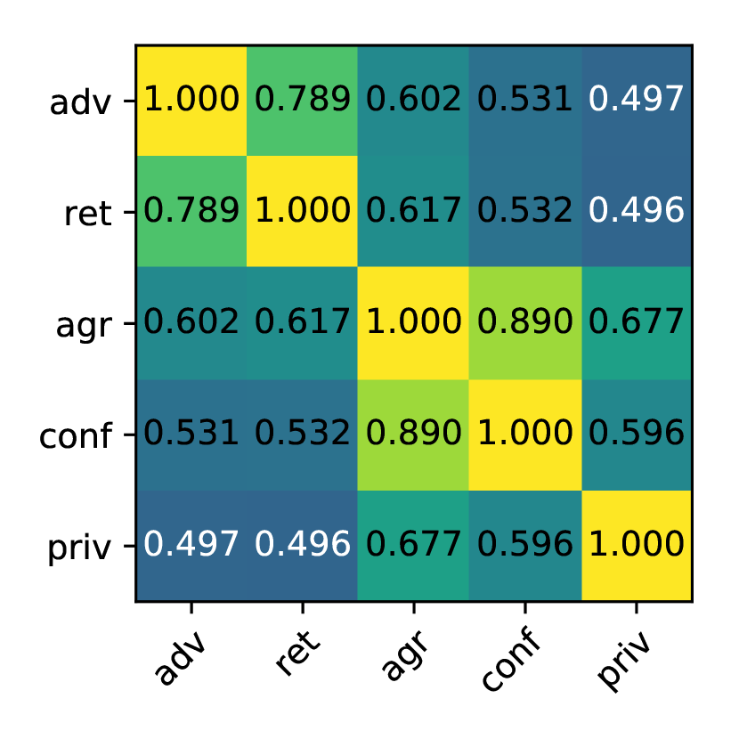
(c) CIFAR-10

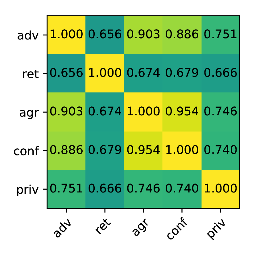
(d) ImageNet

Figure 2: Correlation coefficients for our five prototypicality metrics on four common datasets.

3 Evaluating the Five Different Metrics

As the first step in an evaluation, it is natural to consider to what extent these metrics are different methods of evaluating the same underlying property. We find that the are highly correlated across the four datasets we study: MNIST (LeCun et al., 2010), Fashion-MNIST (Xiao et al., 2017), CIFAR-10 (Krizhevsky & Hinton, 2009), and ImageNet (Russakovsky et al., 2015). In particular, we observe a strong correlation between the adversarial distance and holdout retraining metrics, which is of independent interest: the holdout retraining metric could serve as a substitute for adversarial distance in tasks where adversarial examples are ill-defined.

Our metrics are widely applicable, as they are not specific to any learning task or model (some, like ret and priv might be applicable even to unsupervised learning), and experimentally we have confirmed that the metrics are model-agnostic in the sense that they give overall the same results despite large changes in hyperparameters or even the model architecture. We also show that our metrics are consistent with human perception of representativeness.

An important application of our metrics is that studying their (relatively rare) disagreements allow us to inspect datasets at scale. In particular, we show how to identify two types of examples: memorized exceptions and uncommon submodes. They can be used to form an understanding of performance at training and test time that is more precise than what an accuracy measurement can offer. (Due to space constraints, experimental results supporting some of the above observations are given in the Appendix.)

We release the full results of running our metrics on each of the four datasets in the Appendix; we encourage the interested reader to examine the results, we believe the results speak for themselves.

	MNIST	Fashion-MNIST	CIFAR-10
Pick Worst
Pick Best

Table 1: Results of a human study of Mechanical Turk workers selecting the best or worst example among a random collection of 9 training-data images. For each metric, the tables show what percent of workers selected examples in each 10% split of the metric’s sorted ranking (e.g., when shown MNIST digits, $25\%$ human workers selected as worst an example that fell in the bottom $10\%$ of examples as ranked by the adv metric.

3.1 Correlations Between Metrics

Figure 2 shows the correlation coefficients computed pairwise between each of our metrics for all our datasets, (the tables are symmetric across the diagonal). The metrics are overall strongly correlated, and the differences in correlation are informative. Unsurprisingly, since they measure very similar properties, the agr (ensemble agreement) and the conf (model confidence) show the highest correlation,

However, somewhat unexpectedly, we find that the adv metric (adversarial robustness) correlates very strongly with the ret metric (retraining distance) on the smaller three datasets. This is presumably because these two metrics both measure the distance to a model’s decision boundary—even though adv measures this distance by perturbing each example while ret measures how the evaluation of each example is affected when models’ decision boundaries themselves are perturbed. On ImageNet, adv is most strongly correlated with ensemble agreement and model confidence; we hypothesize this is due to the fact that ImageNet is a much more challenging task and therefore the distance to the decision boundary can be best approximated by the initial model confidence, unlike on MNIST where most datapoints (even incorrectly labeled) are assigned probability $0.999$ or higher.

This strong correlation between adv and ret is a new result that may be of independent interest and some significance. Measurement of adversarial distance is a useful and highly-utilize technique, but it is undefined or ill-defined on many learning tasks and its computation is difficult, expensive, and hard to calibrate. On the other hand, given any holdout dataset and any measure of divergence, the ret metric we define in Section 2.1 should be easily computable for any ML model or task.

3.2 Qualitative Evaluation Inspection and Human Study

Clearly these metrics do consistently measure some quantity which is inspired by how well represented individual examples are, but we have not yet provided evidence that it does so. To do this, we will show that our methods for identifying examples that are well represented in the dataset match human intuition for examples that are of a high quality.

To begin, we perform a subjective visual inspection of how the different metrics rank the example training and test data on different datasets. As a representative example, Figure 1 (Page 1) and the figures in Appendix 7 confirm that there is an obviously apparent difference between the two extremes on the MNIST, Fashion-MNIST, and CIFAR-10 training examples (ImageNet examples are given in the Appendix).

To more rigorously validate and quantify how our metrics correlate with human perception, we performed an online human study using Amazon’s Mechanical Turk service. We presented human evaluators a collection of images (all of one class) from the MNIST, Fashion-MNIST, or CIFAR-10 datasets. We asked the evaluator to select either the image that was most or least representative of the class. In the study, 400 different human evaluators assessed over 100,000 images. At a high level, the human evaluators largely agreed that the images selected by our algorithms as most representative do in fact match human intuition.

Concretely, in this study (an image of the study form is given in the Appendix, Section 9), each human evaluator saw a 3x3 grid of 9 random images and was asked to pick the worst image—or the best image—and this was repeated multiple times. Evaluators exclusively picked either best or worst images and were only shown random images from one output class under a heading with the label name of that class; thus one person would pick only the best MNIST digits “7” while another picked only the worst CIFAR-10 “cars.” (As dictated by good study design, we inserted “Gold Standard” questions with known answers to catch workers answering randomly or incorrectly, eliminating the few such workers from our data.) For all datasets, picking non-representative images proved to be the easier task: in a side study where 50 evaluators were shown the same identical 3x3 grids, agreement was $80\%$ on the worst image but only $27\%$ on the best image (random choice would give $11\%$ agreement).

The results of our human study are presented in Table 1. The key takeaway is that the evaluator’s assessment is correlated with each one of our metrics: evaluators mostly picked the not well-represented images as the worst examples and examples that were better represented as being the best.

3.3 Comparing Metrics and their Characteristics

Figure 3: Scatter plot comparing the adv vs. conf ranks on the MNIST test set. Notice clusters of digits, for examples the 1 class that has extremely high average confidence (i.e., they are easy to classify) but low adversarial distance (i.e., are easy to perturb to other classes).

Because our five metrics are not perfectly correlated, there are likely to be many examples that are determined to be well-represented under one metric but not under another, as a consequence of the fact that each metric defines “well-represented” differently. To quantify the number and types of those differences we can try looking at their visual correlation in a scatter plot; doing so can be informative, as can be seen in Figure 3(a) where the easily-learned, yet fragile, examples of class “1” in MNIST models have high confidence but low adversarial robustness. The results show substantial disagreement between metrics.

To understand disagreements, we can consider examples that are well represented in one metric but not in others, first combining the union of adv and ret into a single boundary metric, and the union of adv and ret into an ensemble metric, because of their high correlation.

Memorized exceptions:  Recalling the unusual dress-looking “shirt” of Figure 1, and how it seemed to have been memorized with high confidence, we can intersect the top 25% well represented ensemble images with the bottom-half outliers in both the boundary and priv metrics.

Figure 4: Exceptional “shirts.”

For the Fashion-MNIST “shirt” class, this set—visually shown in Figure 4 on the right—includes not only the dress-looking example but a number of other atypical “shirt” images, including some looking like shorts. Also apparent in the set are a number of T-shirt-like and pullover-like images, which are misleading, given the other output classes of Fashion-MNIST. For these sets, which are likely to include spurious, erroneously-labeled, and inherently ambiguous examples, we use the name memorized exceptions because they must be memorized as exceptions for models to have been able to reach very high confidence during training. Similarly, Figure 5(a) shows a large (green) cluster of highly ambiguous boot-like sneakers, which appear indistinguishable from a cluster of memorized exceptions in the Fashion-MNIST “ankle boot” class (see Appendix 7).

Uncommon submodes:  On the other hand, the priv metric is based on differentially-private learning which ensures that no small group of examples can possibly be memorized: the privacy stems from adding noise and attenuating gradients in a manner that will mask the signal from rare examples during training. This suggests that we can find uncommon submodes of the examples in learning tasks by intersecting the bottom-most outlier examples on the priv metric with the union of most well-represented in the boundary and ensemble metrics. Figure 5(b) shows uncommon submodes discovered in MNIST using the 25% lowest outliers on priv and top 50% well-represented on other metrics. Notably, all of the “serif 1s” in the entire MNIST training set are found as a submode.

Canonical prototypes:  Finally, we can simply consider the intersection of the sets of all the most represented examples in all of our metrics. The differences between our metrics should ensure that this intersection is free of spurious or misleading examples; yet, our experiments and human study suggest the set will provide good coverage. Hence, we call this set canonical prototypes. Figure 5(c) shows the airplanes that are canonical prototypes in CIFAR-10.

(a) Memorized exceptions in the Fashion-MNIST “sneaker” class.

(b) Uncommon submodes found within the MNIST “1” class.

(c) Canonical prototypes in the CIFAR-10 “airplane” class.

Figure 5: Our metrics’ sets reveal interesting examples, which can be clustered.

(a) MNIST

(b) Fashion-MNIST

(c) CIFAR-10

Figure 6: Final test accuracy of a model after trained on $5,000$ training examples consecutively ranked by the adv metric (so that training on the least representative examples are that the 0th percentile, and the most representative at the 100th percentile). See text for full details. Given only $5,000$ training examples, on MNIST (subplot (a)) training on the outliers is always better, however for Fashion-MNIST (b) and CIFAR-10 (c) it is preferable to train using neither the most nor least well-represented examples, but those in the middle.

(d) MNIST

(e) Fashion-MNIST

(f) CIFAR-10

Figure 7: Final test accuracy of a model after trained on a varrying percentage of training data as sorted by the adv metric. The blue solid lines correspond to final test accuracy when the training data consists of only the $x\%$ least well-represented examples, and growing to the most represented. The orange solid line corresponds to training on the $x\%$ most most well represented examples; the orange dashed line corresponds to when testing only on the top $50\%$ most well-represented test points. See text for full details.

To further aid interpretability in Figures 4 and 5, we perform a combination of dimensionality reduction and clustering. We apply t-SNE (Maaten & Hinton, 2008) on the pixel space (for MNIST and Fashion-MNIST) or ResNetv2 feature space (for CIFAR10) to project the example sets into two dimensions, and cluster with HDBSCAN (Campello et al., 2013), a hierarchical and density-based clustering algorithm which does not try to assign all points to clusters—which not only can improve clusters but also identify spurious data. We believe that other types of data projection and clustering could also be usefully applied to our metrics, and offer significant insight into ML datasets. (See Appendix 11 for this section’s figures shown larger.)

4 Utilizing Well-Represented Examples

Our metrics enable us to inspect datasets at scale and identify examples in the training and test sets that are of particular importance to evaluating a model’s performance. For instance, imagine we observe that a non-private model performs better than a private model because the private model is unable to classify uncommon submodes correctly. This is desirable because it is harder to protect the privacy of examples that are not well-represented in the training data. However, if one were to limit their evaluation to simply reporting accuracy, we would conclude that the privacy-preserving model performs “worse” while this is not necessarily the case.

Beyond such applications that provide insights into learning and inference, we now show that our metrics for sorting examples according to how well-represented they are can also be integrated directly in learning procedures to improve them. Namely, we look at three model properties: sample complexity, accuracy, or robustness.

4.1 Curriculum Learning

We perform two experiments on the three datasets to investigate whether it is better to train on the the well-represented examples or the outliers—exploring the “train on hard data” vs. “train on easy data” question of curriculum learning (Ren et al., 2018). To begin, we order all training data according to our adv metric.

Experiment 1. First, we experiment with training on splits of $5,000$ training examples (approximately $10\%$ of the training data) chosen by taking the $k$-th most well-represented example to the ($k$+5000)-th most well-represented, for different values of $k$. As shown in Figure 7, we find that the index $k$ that yields the most accurate model varies substantially across the datasets and tasks. (In the plot, the x-axis is given in a percentile from $0$ to $100$, obtained by dividing $k$ by the size of the dataset.) For example, initially we train a model on only the $5,000$ least represented examples and record the models’s final test accuracy; for MNIST this accuracy is nearly $99\%$ already. However, for CIFAR-10 it is preferable to take $5,000$ examples starting at the 60th percentile—that is, examples ordered from $30,000$ to $35,000$ by the adv metric reach a test accuracy of $77\%$.

To summarize the results, on MNIST, training on the outlier examples gives the highest accuracy; conversely, on Fashion-MNIST and CIFAR-10, training on examples that are better represented gives the highest accuracy. We conjecture this is due to the dataset complexity: because nearly all of MNIST is very easy, it makes sense to train on the hardest, most outlier examples. However, because Fashion-MNIST and CIFAR-10 CIFAR-10 are comparably difficult, training on the most well-represented examples is better given a limited amount of training data: it is simply too hard to learn on only the least representative training examples.

Notably, many of the CIFAR-10 and Fashion-MNIST outliers appear to be inherently misleading or ambiguous examples, and several are simply erroneously labeled. We find that about $10\%$ of the first 5,000 outliers meet our definition of memorized exceptions. Also, we find that inserting 10% label noise causes model accuracy to decrease by about 10%, regardless of the split trained on—i.e., that to achieve high accuracy on small training data erroneous and misleading outliers must be removed—and explaining the low accuracy shown on the left in the graph of Figures 6(b) and  6(c).

Experiment 2. For our second experiment, we ask: is it better to train on the $k$-most or $k$-least well-represented examples? That is, the prior experiment assumed the amount of data is fixed, and we must choose which percentile of data to use. Now, we examine what the best strategy is to apply if we must choose either a prefix or a suffix of the training data as ordered by our adv metric.

The results are given in Figure 7. Again, we find the answer depends on the dataset. On MNIST, training on the $k$-least represented examples is always better for any $k$ than training on the $k$-most represented examples. However, on Fashion-MNIST and CIFAR-10, training on the well-represented examples is better when $k$ is small, but as soon as we begin to collect more than roughly $10,000$ examples for Fashion-MNIST or $20,000$ for CIFAR-10, training on the outliers begins to give more accurate models. However, we find that training only on the most well-represented examples found in the training data gives extremely high test accuracy on the well-represented examples found in the test data.

This evidence supports our hypothesis that training on difficult, but not impossibly difficult, training data is of most value. The harder the task, the more useful well-represented training examples are.

Also shown in Figure 7 is the final test accuracy of a model when only evaluated on the well-represented test examples. Here, we find that the test accuracy is subsantially higher.

4.2 Decision Boundary Analysis

While training exclusively on the well-represented examples often gives inferior accuracy compared to training on the outliers, the former has the benefit of obtaining models with simpler decision boundaries. Thus, it is natural to ask whether training on well represented examples gives models that are more robust to adversarial examples (Szegedy et al., 2013). In fact, prior work has found that discarding outliers from the training data can help with both classifying and detecting adversarial examples (Liu et al., 2018).

To show that simpler boundaries can lead to somewhat higher robustness, we train models on fixed-sized subsets of the data where include $5,000$ training points either from the well-represented training examples or those that are not. For each model, we then compute the mean $\ell_{\infty}$ adversarial distance needed to find adversarial examples. As shown in Figure 11 in the Appendix, the Fashion-MNIST and CIFAR-10 models that are trained on well well represented examples are more robust to adversarial examples than those trained on a slice of training data that is mostly made up of outliers. However, these models trained on a slice of $5,000$ well-represented examples remain comparably robust to a baseline model trained on the entire data.

5 Related Work

Prototypes.

At least since the work of Zhang (1992) which was based on intra- and inter-concept similarity, prototypes have been examined using several metrics derived from the intuitive notion that one could find “quintessential observations that best represent clusters in a dataset” (Kim et al., 2014). Several more formal variants of this definition were proposed in the literature—along with corresponding techniques for finding prototypes. Kim et al. (2016) select prototypes according to their maximum mean discrepancy with the data, which assumes the existence of an appropriate kernel for the data of interest. Li et al. (2017) circumvent this limitation by prepending classifiers with an autoencoder projecting the input data on a manifold of reduced dimensionality. A prototype layer, which serves as the classifier’s input, is then trained to minimize the distance between inputs and a set of prototypes on this manifold. While this method improves interpretability by ensuring that prototypes are central to the classifier’s logic, it does require that one modify the model’s architecture. Instead, metrics considered in our manuscript all operate on existing architectures. Stock & Cisse (2017) proposed to use distance to the boundary—approximately measured with an adversarial example algorithm—as a proxy for prototypicality.

Other interpretability approaches.

Prototypes enable interpretability because they provide a subset of examples that summarize the original dataset and best explain a particular decision made at test time (Bien & Tibshirani, 2011). Other approaches like saliency maps instead synthesize new inputs to visualize what a neural network has learned. This is typically done by gradient descent with respect to the input space (Zeiler & Fergus, 2014; Simonyan et al., 2013). Because they rely on model gradients, saliency maps can be fragile and only locally applicable (Fong & Vedaldi, 2017).

Beyond interpretability, prototypes are also motivated by additional use cases, some of which we discussed in Section 4. Next, we review related work in two of these applications: namely, curriculum learning and reducing sample complexity.

Curriculum learning.

Based on the observation that the order in which training data is presented to the model can improve performance (e.g., convergence) of optimization during learning and circumvent limitations of the dataset (e.g., data imbalance or noisy labels), curriculum learning seeks to find the best order in which to analyze training data (Bengio et al., 2009). This first effort further hypothesizes that easy-to-classify samples should be presented early in training while complex samples gradually inserted as learning progresses. While Bengio et al. (2009) assumed the existence of hard-coded curriculum labels in the dataset, Chin & Liang (2017) sample an order for the training set by assigning each point a sampling probability proportional to its leverage score—the distance between the point and a linear model fitted to the whole data. Instead, we use metrics that also apply to data that cannot be modeled linearly.

The curriculum may also be generated online during training, so as to take into account progress made by the learner (Kumar et al., 2010). For instance, Katharopoulos & Fleuret (2017) train an auxiliary LSTM model to predict the loss of training samples, which they use to sample a subset of training points analyzed by the learner at each training iteration. Similarly, (Jiang et al., 2017) have an auxiliary model predict the curriculum. This auxiliary model is trained using the learner’s current feature representation of a smaller holdout set of data for which ground-truth curriculum is known.

However, as reported in our experiments, training on easy samples is beneficial when the dataset is noisy, whereas training on hard examples is on the contrary more effective when data is clean. These observations oppose self-paced learning (Kumar et al., 2010) with hard example mining (Shrivastava et al., 2016). Several strategies have been proposed to perform better in both settings. Assuming the existence of a holdout set as well, Ren et al. (2018) assign a weight to each training example that characterizes the alignment of both the logits and gradients of the learner on training and heldout data. Chang et al. (2017) propose to train on points with high prediction variance or whose average prediction is close from the decision threshold. Both the variance and average are estimated by analyzing a sliding window of the history of prediction probabilities throughout training epochs.

Sample complexity.

Prototypes of a given task share some intuition with the notion of coresets (Agarwal et al., 2005; Huggins et al., 2016; Bachem et al., 2017; Tolochinsky & Feldman, 2018) because both prototypes and coresets describe the dataset in a more compact way—by returning a (potentially weighted) subset of the original dataset. For instance, clustering algorithms may rely on both prototypes (Biehl et al., 2016) or coresets (Biehl et al., 2016) to cope with the high dimensionality of a task. However, prototypes and coresets differ in essential ways. In particular, coresets are defined according to a metric of interest (e.g., the loss that one would like to minimize during training) whereas prototypes are independent of any machine-learning aspects as indicated in our list of desirable properties for prototypicality metrics from Section 2.

Taking a different approach, Wang et al. (2018) apply influence functions (Koh & Liang, 2017) to discard training inputs that do not affect learning. Conversely, for MNIST, we found in our experiments that removing individual training examples did not have a measurable impact on the predictions of individual test examples. Specifically, we trained many models to 100% training accuracy where we left one training example out for each model. There was no statistically significant difference between the models predictions on each individual test example

6 Conclusion

This paper explores metrics for gaining insight into the properties of datasets commonly used for training deep learning models. We develop five metrics and find that humans agree that the rankings computed capture human intuition behind what is meant by a good representative example of the class.

When the metrics disagree on how well-represented an example is, we can often learn something interesting about that example. This helps forming an understanding of the performance of ML models that goes beyond measuring test accuracy. For instance, by identifying memorized exceptions in the test data, we may not weight mistakes that models make on these points as important as mistakes on canonical prototypes. Further, by identifying uncommon submodes we can learn where collecting training points will be useful. We find that models trained on well-represented examples often have simpler decision boundaries and are thus slightly more adversarially robust, however training only on the most represented often yields inferior accuracy compared to training on outliers.

We believe that exploring other metrics for assessing properties of datasets and developing methods for using them during training is an important area of future work, and hope that our analysis will be useful towards that end goal.

Appendix

7 Figures of outliers

The following are training examples from MNIST, FashionMNIST, and CIFAR10 that are identified as most outlier (left of the red bar) or prototypical (right of the green bar). Images are presented in groups by class. Each row in these groups corresponds to one of the five metrics in Section 2.1.

7.1 MNIST extreme outliers

All MNIST results were obtained with a CNN made up of two convolutional layers (each with kernel size of 5x5 and followed by a 2x2 max-pooling layer) and a fully-connected layer of 256 units. It was trained with Adam at a learning rate of $10^{-3}$ with a $10^{-3}$ decay. When an ensemble of models was needed (e.g., for the agr metric), these were obtained by using different random initializations.

adv
ret
agr
conf
priv

adv
ret
agr
conf
priv

adv
ret
agr
conf
priv

adv
ret
agr
conf
priv

adv
ret
agr
conf
priv

adv
ret
agr
conf
priv

adv
ret
agr
conf
priv

adv
ret
agr
conf
priv

adv
ret
agr
conf
priv

adv
ret
agr
conf
priv

7.2 Fashion-MNIST extreme outliers

The Fashion-MNIST model architecture is identical to the one used for MNIST. It was also trained with the same optimizer and hyper-parameters.

adv
ret
agr
conf
priv

adv
ret
agr
conf
priv

adv
ret
agr
conf
priv

adv
ret
agr
conf
priv

adv
ret
agr
conf
priv

adv
ret
agr
conf
priv

adv
ret
agr
conf
priv

adv
ret
agr
conf
priv

adv
ret
agr
conf
priv

adv
ret
agr
conf
priv

7.3 CIFAR extreme outliers

All CIFAR results were obtained with a ResNetv2 trained on batches of $32$ points with the Adam optimizer for $100$ epochs at an initial learning rate of $10^{-3}$ decayed down to $10^{-4}$ after 80 epochs. We adapted the following data augmentation and training script: https://raw.githubusercontent.com/keras-team/keras/master/examples/cifar10_resnet.py When an ensemble of models was needed (e.g., for the agr metric), these were obtained by using different random initializations.

adv
ret
agr
conf
priv

adv
ret
agr
conf
priv

adv
ret
agr
conf
priv

adv
ret
agr
conf
priv

adv
ret
agr
conf
priv

adv
ret
agr
conf
priv

adv
ret
agr
conf
priv

adv
ret
agr
conf
priv

adv
ret
agr
conf
priv

adv
ret
agr
conf
priv

7.4 ImageNet extreme outliers

The following pre-trained ImageNet models were used: DenseNet121, DenseNet169, DenseNet201 InceptionV3, InceptionResNetV2, Large NASNet, Mobile NASNet, ResNet50, VGG16, VGG19, and Xception. They are all found in the Keras library: https://keras.io/applications.

adv
agr
conf

adv
agr
conf

adv
agr
conf

adv
agr
conf

adv
agr
conf

adv
agr
conf

adv
agr
conf

adv
agr
conf

adv
agr
conf

adv
agr
conf

8 Accuracy on well represented data when training only on well represented data

The three matrices that follow respectively report the accuracy of MNIST, Fashion-MNIST and CIFAR-10 models learned on training examples with varying degrees of prototypicality and evaluated on test examples also with varying degrees of prototypicality. Specifically, the model used to compute cell $(i,j)$ of a matrix is learned on training data that is ranked in the $i^{th}$ percentile of  adv prototypicality. The model is then evaluated on the test examples whose adv prototypicality falls under the $j^{th}$ prototypicality percentile. For all datasets, these matrices show that performing well on non-outliers is possible even when the model is trained on outliers. For MNIST, this shows again that training on outliers provides better performance across the range of test data (from outliers to well represented examples). For Fashion-MNIST and CIFAR-10, this best performance is achieved by training on examples that are neither prototypical nor outliers.

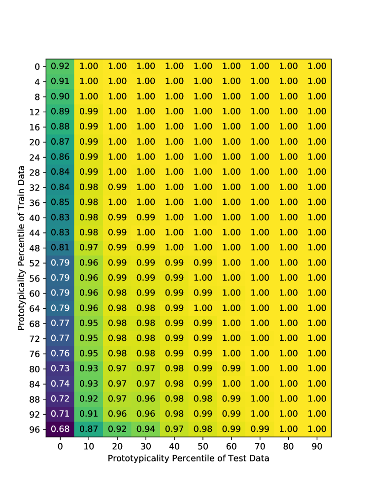
Figure 8: MNIST

Figure 9: Fashion-MNIST

Figure 10: CIFAR-10

9 Human Study Example

We presented Mechanical Turk taskers with the following webpage, asking them to select the worst image of the nine in the grid.

10 Adversarial robustness of model trained on only well represented examples

(a) MNIST

(b) Fashion-MNIST

(c) CIFAR-10

Figure 11: The blue curves indicate the training accuracy of models trained on slices of $5,000$ examples selected according to their prototypicality—as reported on the x-axis. A baseline, obtained by training the model on the entire dataset is indicated by the dotted-orange line. Models trained on well represented examples on Fashion-MNIST and CIFAR-10 are $2\times$ more robust to adversarial examples, when training on slices of $5,000$ prototypical examples as opposed to slices of $5,000$ outlier examples. On MNIST there is no significant difference; almost all examples are good.

11 Revealing and clustering interesting examples and submodes

Figure 12: Uncommon submodes found within the MNIST “1” class, and their HDBSCAN clusters.

Figure 13: Memorized exceptions in the Fashion-MNIST “sneakers,” and their HDBSCAN clusters.

Figure 14: Memorized exceptions in the Fashion-MNIST “shirts,”, and their HDBSCAN clusters.

Figure 15: Canonical prototypes in the CIFAR-10 “airplane” class.

12 Comparing density of our metrics for different metrics over the output classes of all learning tasks

13 All memorized exceptions for all Fashion-MNIST classes

Below are all the memorized exceptions, as defined in the body of the paper, for all Fashion-MNIST output classes:

• Tshirt/top

• Trouser

• Pullover

• Dress

• Coat

• Sandal

• Shirt

• Sneaker

• Bag

• Ankle boot

14 ImageNet Memorized Exceptions

See pages - of figures/memorized_imagenet.pdf

References

- Abadi et al. (2016) Martin Abadi, Andy Chu, Ian Goodfellow, H Brendan McMahan, Ilya Mironov, Kunal Talwar, and Li Zhang. Deep learning with differential privacy. In Proceedings of the 2016 ACM SIGSAC Conference on Computer and Communications Security, pp. 308–318. ACM, 2016.
- Agarwal et al. (2005) Pankaj K Agarwal, Sariel Har-Peled, and Kasturi R Varadarajan. Geometric approximation via coresets. Combinatorial and computational geometry, 52:1–30, 2005.
- Bachem et al. (2017) Olivier Bachem, Mario Lucic, and Andreas Krause. Practical coreset constructions for machine learning. arXiv preprint arXiv:1703.06476, 2017.
- Bengio et al. (2009) Yoshua Bengio, Jérôme Louradour, Ronan Collobert, and Jason Weston. Curriculum learning. In Proceedings of the 26th annual international conference on machine learning, pp. 41–48. ACM, 2009.
- Biehl et al. (2016) Michael Biehl, Barbara Hammer, and Thomas Villmann. Prototype-based models in machine learning. Wiley Interdisciplinary Reviews: Cognitive Science, 7(2):92–111, 2016.
- Bien & Tibshirani (2011) Jacob Bien and Robert Tibshirani. Prototype selection for interpretable classification. The Annals of Applied Statistics, pp. 2403–2424, 2011.
- Biggio et al. (2013) Battista Biggio, Igino Corona, Davide Maiorca, Blaine Nelson, Nedim Šrndić, Pavel Laskov, Giorgio Giacinto, and Fabio Roli. Evasion attacks against machine learning at test time. In Joint European conference on machine learning and knowledge discovery in databases, pp. 387–402. Springer, 2013.
- Campello et al. (2013) Ricardo JGB Campello, Davoud Moulavi, and Jörg Sander. Density-based clustering based on hierarchical density estimates. In Pacific-Asia conference on knowledge discovery and data mining, pp. 160–172. Springer, 2013.
- Carlini & Wagner (2017) Nicholas Carlini and David Wagner. Towards evaluating the robustness of neural networks. In 2017 IEEE Symposium on Security and Privacy (SP), pp. 39–57. IEEE, 2017.
- Chang et al. (2017) Haw-Shiuan Chang, Erik Learned-Miller, and Andrew McCallum. Active bias: Training more accurate neural networks by emphasizing high variance samples. In Advances in Neural Information Processing Systems, pp. 1002–1012, 2017.
- Chin & Liang (2017) Hui Han Chin and Paul Pu Liang. Leverage score ordering. In Advances in Neural Information Processing Systems, 2017.
- Fong & Vedaldi (2017) Ruth C Fong and Andrea Vedaldi. Interpretable explanations of black boxes by meaningful perturbation. arXiv preprint arXiv:1704.03296, 2017.
- Huggins et al. (2016) Jonathan Huggins, Trevor Campbell, and Tamara Broderick. Coresets for scalable bayesian logistic regression. In Advances in Neural Information Processing Systems, pp. 4080–4088, 2016.
- Jiang et al. (2017) Lu Jiang, Zhengyuan Zhou, Thomas Leung, Li-Jia Li, and Li Fei-Fei. Mentornet: Regularizing very deep neural networks on corrupted labels. arXiv preprint arXiv:1712.05055, 2017.
- Katharopoulos & Fleuret (2017) Angelos Katharopoulos and François Fleuret. Biased importance sampling for deep neural network training. arXiv preprint arXiv:1706.00043, 2017.
- Kim et al. (2014) Been Kim, Cynthia Rudin, and Julie A Shah. The bayesian case model: A generative approach for case-based reasoning and prototype classification. In Advances in Neural Information Processing Systems, pp. 1952–1960, 2014.
- Kim et al. (2016) Been Kim, Rajiv Khanna, and Oluwasanmi O Koyejo. Examples are not enough, learn to criticize! criticism for interpretability. In Advances in Neural Information Processing Systems, pp. 2280–2288, 2016.
- Koh & Liang (2017) Pang Wei Koh and Percy Liang. Understanding black-box predictions via influence functions. arXiv preprint arXiv:1703.04730, 2017.
- Krizhevsky & Hinton (2009) Alex Krizhevsky and Geoffrey Hinton. Learning multiple layers of features from tiny images. Technical report, Citeseer, 2009.
- Kumar et al. (2010) M Pawan Kumar, Benjamin Packer, and Daphne Koller. Self-paced learning for latent variable models. In Advances in Neural Information Processing Systems, pp. 1189–1197, 2010.
- Kurakin et al. (2016) Alexey Kurakin, Ian Goodfellow, and Samy Bengio. Adversarial examples in the physical world. arXiv preprint arXiv:1607.02533, 2016.
- LeCun et al. (2010) Yann LeCun, Corinna Cortes, and CJ Burges. Mnist handwritten digit database. AT&T Labs [Online]. Available: http://yann. lecun. com/exdb/mnist, 2, 2010.
- Li et al. (2017) Oscar Li, Hao Liu, Chaofan Chen, and Cynthia Rudin. Deep learning for case-based reasoning through prototypes: A neural network that explains its predictions. arXiv preprint arXiv:1710.04806, 2017.
- Liu et al. (2018) Yongshuai Liu, Jiyu Chen, and Hao Chen. Less is more: Culling the training set to improve robustness of deep neural networks. arXiv preprint arXiv:1801.02850, 2018.
- Maaten & Hinton (2008) Laurens van der Maaten and Geoffrey Hinton. Visualizing data using t-sne. Journal of machine learning research, 9(Nov):2579–2605, 2008.
- Papernot et al. (2016) Nicolas Papernot, Martín Abadi, Úlfar Erlingsson, Ian Goodfellow, and Kunal Talwar. Semi-supervised knowledge transfer for deep learning from private training data. arXiv preprint arXiv:1610.05755, 2016.
- Ren et al. (2018) Mengye Ren, Wenyuan Zeng, Bin Yang, and Raquel Urtasun. Learning to reweight examples for robust deep learning. arXiv preprint arXiv:1803.09050, 2018.
- Russakovsky et al. (2015) Olga Russakovsky, Jia Deng, Hao Su, Jonathan Krause, Sanjeev Satheesh, Sean Ma, Zhiheng Huang, Andrej Karpathy, Aditya Khosla, Michael Bernstein, et al. Imagenet large scale visual recognition challenge. International Journal of Computer Vision, 115(3):211–252, 2015.
- Shrivastava et al. (2016) Abhinav Shrivastava, Abhinav Gupta, and Ross Girshick. Training region-based object detectors with online hard example mining. In Proceedings of the IEEE Conference on Computer Vision and Pattern Recognition, pp. 761–769, 2016.
- Simonyan et al. (2013) Karen Simonyan, Andrea Vedaldi, and Andrew Zisserman. Deep inside convolutional networks: Visualising image classification models and saliency maps. arXiv preprint arXiv:1312.6034, 2013.
- Stock & Cisse (2017) Pierre Stock and Moustapha Cisse. Convnets and imagenet beyond accuracy: Explanations, bias detection, adversarial examples and model criticism. arXiv preprint arXiv:1711.11443, 2017.
- Szegedy et al. (2013) Christian Szegedy, Wojciech Zaremba, Ilya Sutskever, Joan Bruna, Dumitru Erhan, Ian Goodfellow, and Rob Fergus. Intriguing properties of neural networks. arXiv preprint arXiv:1312.6199, 2013.
- Tolochinsky & Feldman (2018) Elad Tolochinsky and Dan Feldman. Coresets for monotonic functions with applications to deep learning. arXiv preprint arXiv:1802.07382, 2018.
- Wang et al. (2018) Tianyang Wang, Jun Huan, and Bo Li. Data dropout: Optimizing training data for convolutional neural networks. arXiv preprint arXiv:1809.00193, 2018.
- Xiao et al. (2017) Han Xiao, Kashif Rasul, and Roland Vollgraf. Fashion-mnist: a novel image dataset for benchmarking machine learning algorithms, 2017.
- Zeiler & Fergus (2014) Matthew D Zeiler and Rob Fergus. Visualizing and understanding convolutional networks. In European conference on computer vision, pp. 818–833. Springer, 2014.
- Zhang (1992) Jianping Zhang. Selecting typical instances in instance-based learning. In Proceedings of the Ninth International Workshop on Machine Learning, ML92, pp. 470–479, 1992. URL http://dl.acm.org/citation.cfm?id=141975.142091.