X-ray diffractive imaging of controlled gas-phase molecules: Toward imaging of dynamics in the molecular frame

Abstract

We report experimental results on the diffractive imaging of three-dimensionally aligned 2,5-diiodothiophene molecules. The molecules were aligned by chirped near-infrared laser pulses, and their structure was probed at a photon energy of 9.5 keV ($\lambda\approx 130~{}\text{pm}$) provided by the Linac Coherent Light Source. Diffracted photons were recorded on the CSPAD detector and a two-dimensional diffraction pattern of the equilibrium structure of 2,5-diiodothiophene was recorded. The retrieved distance between the two iodine atoms agrees with the quantum-chemically calculated molecular structure to within 5 %. The experimental approach allows for the imaging of intrinsic molecular dynamics in the molecular frame, albeit this requires more experimental data, which should be readily available at upcoming high-repetition-rate facilities.

I Introduction

Coherent diffractive imaging has become a widespread tool for a variety of different experiments and samples, e. g., ranging from the solid state to the gas phase and from small molecules to large protein crystals. The idea is that the structure of a system, for example, a molecule, protein, or virus, determines its function. Thus, extracting structural information in the static or time-dependent domain helps to drastically increase the knowledge of fundamental processes in nature. The imaging of structure can be performed by the diffraction of electrons or x-rays off the sample molecules. Electron diffraction has been used for decades to determine the structure of small gas-phase molecules Allen and Sutton (1950); Hargittai and Hargittai (1988), making use of the electrons’ much higher coherent scattering cross section Henderson (1995). X-rays have a lower scattering cross section than electrons and hence penetrate more deeply into the sample. Consequently, x-ray diffraction is often used to image much denser crystalline samples, which, due to the many identical, oriented molecules, provides a coherent amplification of the signal over the noise at the Bragg diffraction angles. This led, for instance, to the confirmation of the planar structure of benzene Lonsdale (1929), the structure of penicillin Crowfoot et al. (1949), and the structure of the DNA double helix Watson and Crick (1953). Today, crystallography is still a very successful approach to probe the structure of, e. g., proteins, protein complexes, and viruses Spence (2017). However, not all molecules can be crystallized and, furthermore, dense crystal packing can constrain molecular conformations and hamper molecular dynamics.

Diffractive imaging of gas-phase molecules is a highly promising tool to unravel the intrinsic molecular dynamics of chemical processes on ultrafast timescales Zewail (2006); Neutze et al. (2000); Filsinger et al. (2011); Barty, Küpper, and Chapman (2013). Time resolved diffraction studies of small gas-phase molecules in the picosecond range were first employed by electron diffraction at the beginning of the 21st century Ihee et al. (2001); Sciaini and Miller (2011) and have been used ever since with laboratory-based electron sources Hensley, Yang, and Centurion (2012); Müller et al. (2015). Recently, much higher time resolution of $\mathord{\sim}100$ fs was achieved by an accelerator-facility based relativistic electron gun Yang et al. (2016, 2018). The development of ultrashort and intense hard x-ray laser pulses generated by x-ray free-electron lasers (XFELs) has also provided the possibility to image structure as well as structural changes of small gas-phase molecules through x-ray diffraction Küpper et al. (2014); Stern et al. (2014); Minitti et al. (2015) on ultrafast (femtosecond) timescales.

To retrieve the three-dimensional (3D) diffraction volume of a molecule, which can be inverted to its 3D structure, knowledge about the relative orientation of the imaged sample(s) with respect to laboratory fixed axes, i. e., the molecular frame, is highly advantageous or simply necessary when averaging data over multiple molecules. In a crystal each molecule is aligned with respect to the crystallographic axes. The crystals usually provide enough scattered photons per XFEL pulse to determine the orientation of the crystal a posteriori and, therefore, the orientation of each molecule Chapman et al. (2011); Spence, Weierstall, and Chapman (2012). This is not possible for single small molecules due to the low number of scattered photons per molecule ($\ll 1$ photons/molecule/pulse). Instead, access to the molecular frame can be achieved by laser alignment of a single molecule or a molecular ensemble Filsinger et al. (2011); Barty, Küpper, and Chapman (2013); Spence and Doak (2004). The finitely-sampled diffraction pattern of a perfectly oriented molecular ensemble is equal to the diffraction pattern of the individual molecule Filsinger et al. (2011),^, because the ensemble is generally lacking translational symmetry – as opposed to a crystal. This has the added benefit that the scattering signal may be averaged over many XFEL shots Stern et al. (2014).

Here, we present results on the diffractive imaging of controlled gas-phase 2,5-diiodothiophene (C₄H₂I₂S) molecules. The data were measured at the coherent x-ray imaging (CXI) instrument Liang et al. (2015) of the Linac Coherent Light Source (LCLS, experiment LG26, October 2014). The molecules were aligned in all three dimensions by an off-resonant, elliptically polarized, linearly chirped near-infrared laser pulse at the full XFEL repetition rate of 120 Hz Kierspel et al. (2015). The aligned molecular ensembles were probed at a photon energy of 9.5 keV ($\lambda\approx 130~{}\text{pm}$), enabling the measurement of intramolecular atomic distances. Approximately 2.2 million individual diffraction patterns of the molecular ensemble have been integrated, and a two-dimensional (2D) diffraction pattern from an ensemble of the three-dimensionally (3D) aligned planar molecules was recorded. The molecular diffraction pattern was compared to the simulated molecular diffraction pattern. The experimental setup was designed to measure ultrafast molecular dynamics on 3D-aligned molecules. Due to large background scatter and the correspondingly limited signal-to-noise ratio of the measurement, we were only able to acquire the diffraction pattern of the static equilibrium structure. The 3D alignment of the molecules was independently verified by velocity map imaging (VMI) Eppink and Parker (1997) of ionic fragments of the molecules Kierspel et al. (2015).

II Experimental setup and procedure

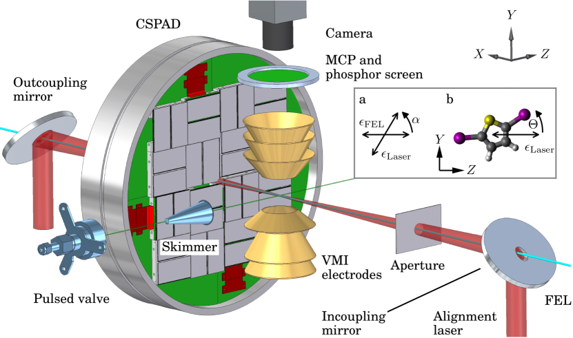
Figure 1: Scheme of the experimental setup showing the pulsed valve, skimmer, and the molecular beam axis indicated by the green line, which is crossed by the XFEL (cyan) and the alignment laser (red). The ion detection system was used to measure the degree of alignment of the molecules, and consists of the VMI electrodes, MCP, phosphor screen, and camera. The CSPAD camera was used to record x-ray photons. Two holey in- and outcoupling mirrors were used to guide the alignment laser through the vacuum chamber, and to ensure collinear propagation with the XFEL. The aperture was used to reduce background from the XFEL beamline on the detector. The inset shows in (a) the definition of the angle $\alpha$, which corresponds to the angle between the polarizations of the XFEL $\epsilon_{\text{XFEL}}$ and the alignment laser $\epsilon_{\text{Laser}}$ and was set to $0\,^{\circ}$ or $66\,^{\circ}$ for the measurement of the degree of alignment or the diffraction pattern, respectively. (b) shows the molecular structure, and schematically defines the angle $\theta$ between $\epsilon_{\text{Laser}}$, and the iodine-iodine (I-I) axis of the molecule.

The experimental setup is sketched in Fig. 1 . A detailed description of the molecular beam parameters as well as the achieved alignment of the molecules is published elsewhere Kierspel et al. (2015). In short, 2,5-diiodothiophene molecules were placed in the sample reservoir of the pulsed Even-Lavie valve Even et al. (2000), which was heated to a temperature of $75\,^{\circ}{}\text{C}$ at the tip of the valve. The molecules were seeded in 80 bar of helium and supersonically expanded into vacuum at a repetition rate of 120 Hz, synchronized to the XFEL repetition rate. A single skimmer (Beam Dynamics, 3 mm diameter) 8 cm downstream of the valve resulted in a 5.2 mm wide molecular beam (full width at half maximum, FWHM) in the interaction zone.

The molecular-beam pulse duration was on the order of 45 µs (FWHM), which led to a peak density of $\mathord{\sim}1\cdot 10^{9}$ molecules per cm³. The molecules were aligned by an in-house chirped-pulse-amplified Ti:Sapphire (TSL) laser system (Coherent) at full XFEL repetition rate. The alignment laser, depicted in red in Fig. 1 , was coupled into the XFEL beam path (cyan) by a holey incoupling mirror to ensure that both beam paths were collinear. An aperture was placed in between the incoupling mirror and the interaction zone to reduce scattering reaching the detectors from sources other than the aligned molecules, such as components in the beamline. The alignment laser pulses were linearly chirped with a pulse duration of 94 ps (FWHM) and a pulse energy of 3.3 mJ, focused to 45 µm (FWHM), which resulted in an estimated peak intensity of $1\cdot 10^{12}~{}\text{W/cm}^{2}$. The alignment laser was elliptically polarized in the $YZ$ plane with an aspect ratio of 3:1, and its polarization could be rotated by a $\lambda$/2 waveplate. The XFEL was linearly polarized along the $Z$ axis and was spatially and temporally placed at the peak intensity of the alignment laser pulse. It was focused to a spot with a width of 12 µm in the horizontal and 3 µm in the vertical axis, and had a pulse duration of approximately 70 fs (FWHM) at photon energy of 9.5 keV, and a pulse energy of approximately 0.64 mJ in the interaction zone, resulting from $4.2\cdot 10^{11}$ photons, a beam line transmission of 80 %, and a focusing-optics transmission of 40 %. The degree of alignment (DOA) of the molecules was probed via ion-momentum imaging perpendicular to the molecular and laser beams in a VMI spectrometer consisting of the VMI electrodes, microchannel plate (MCP), phosphor screen, a fast high-voltage switch (Behlke), and a CCD camera (Adimec Opal) Kierspel et al. (2015). Diffracted photons were measured with the Cornell-SLAC Pixel Array Detector (CSPAD) Hart et al. (2012) 8 cm downstream of the interaction zone. The XFEL and the alignment laser were guided through a central hole of the CSPAD camera. The outcoupling mirror was used to steer the alignment laser outside of the vacuum chamber.

The molecular DOA was probed by rotating the major axis of the alignment laser polarization $\epsilon_{\text{Laser}}$ in the $YZ$ plane such that it was parallel to the VMI detector plane, i. e., $\alpha=0\,^{\circ}$ in Fig. 1 (inset a). The most polarizable axis of the 2,5-diiodothiophene molecules – an axis parallel to the iodine-iodine (I-I) axis – aligned along the major axis of the alignment laser polarization ellipse. The second most polarizable axis aligned along the minor axis of the alignment laser polarization, leading to a 3D-aligned molecular ensemble Stapelfeldt and Seideman (2003); weak 3D orientation might have been present due to the dc electric field from the VMI Nevo et al. (2009), but is not of further relevance. The molecules were Coulomb exploded by the XFEL and VMI spectra of different ionic fragments such as $\text{I}^{+2}$ or $\text{I}^{+3}$ were recorded Kierspel et al. (2015). Due to the high degree of axial recoil for these ionic fragments they allowed for an accurate determination of the DOA Kierspel et al. (2015), typically quantified by $\left<\cos^{2}\!\theta_{\text{2D}}\right>$. Here, $\theta$ is defined as the angle between the major axis of the alignment laser polarization and the axial recoil axis of the molecule, see Fig. 1 (inset b). $\theta_{\text{2D}}$ is the corresponding projected angle in the $XZ$-plane, which is measured by the VMI spectrometer. $\left<\cos^{2}\!\theta_{\text{2D}}\right>$ ranges from 0.5 to 1 for an isotropic and a perfectly aligned molecular ensemble, respectively. When measuring diffraction from the aligned molecular ensemble, we rotated the major axis of the alignment laser polarization to $\alpha=66\,^{\circ}$ as a compromise between the maximum amount of scattered photons at $\alpha=90\,^{\circ}$, and the largest observable scattering vector at $\alpha=45\,^{\circ}$. The molecular DOA was regularly confirmed between diffraction runs by switching between the recording of diffraction images at $\alpha=66\,^{\circ}$ and VMI images at $\alpha=0\,^{\circ}$.

III Simulations

The simulations of the diffraction pattern of 2,5-diiodothiophene were carried out using the CMIdiffract code, which was developed within the CMI group to simulate the diffraction of x-rays or electrons of gas-phase molecules based on the independent atom model Küpper et al. (2014); Stern et al. (2014); Stern (2013); Müller (2016); Kierspel (2016); Müller et al. (2015).

The structure of 2,5-diiodothiophene, which was used to calculate the diffraction pattern, was computed with GAMESS-US Gordon and Schmidt (2005) at the MP2/6-311G** level of theory. Parameters such as molecular beam density, molecular beam width, and the degree of alignment were extracted from the experiment Kierspel et al. (2015) and appropriately considered in the simulations, as were geometric constrains such as the distance from the interaction zone to the CSPAD camera, the size of the detector, the number of incident photons and their energy as well as polarization. Contributions from dissociating molecules in the diffraction pattern are estimated to be on the order of 2 % Küpper et al. (2014); Stern et al. (2014) and are neglected in the calculated diffraction patterns.

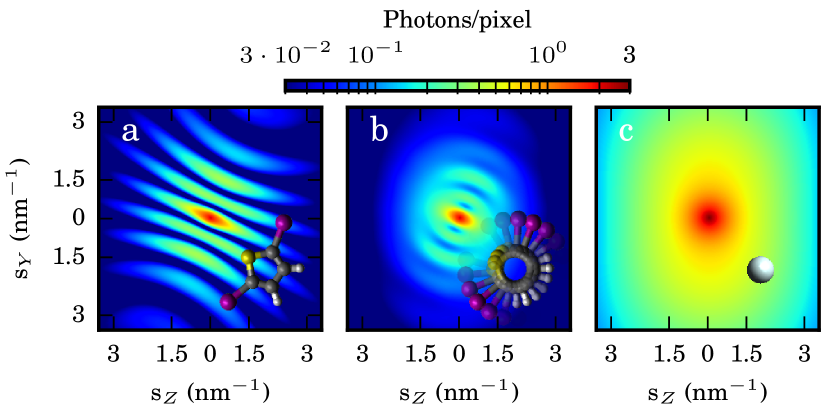
Figure 2: Simulated diffraction pattern of 2,5-diiodothiophene at the location of the CSPAD camera for (a) perfectly aligned and (b) strongly aligned molecules as well as (c) for helium. The insets in the patterns schematically show the molecular structures adapted to the employed DOA and the helium atom.

Fig. 2 a shows the simulated diffraction pattern on the detector for a perfectly aligned molecular ensemble scaled to the number of acquired XFEL pulses for this experiment, i. e., $\mathord{\sim}2.2\times 10^{6}$ XFEL pulses, corresponding to 5.2 h of data acquisition at 120 Hz. The color scale is given by the amount of photons per pixel at a resolution of $1736\times 1736$, and the axes are given as the scattering vector $s$. In the insets sketches of the molecular structure and its orientation for one out of two possible orientations for a 3D-aligned molecule with the given alignment laser polarization, section II , are shown for illustration purposes; in the calculations the correct probability densities are used.

The diffraction patterns show a “double-slit like” interference pattern of the molecule, which is caused by the significantly larger coherent scattering cross section of the iodines compared to the other atoms in the molecule Berger et al. (2010). The increased bending of the fringes towards higher $s$ is due to the projection of the Ewald’s sphere onto a flat detector surface. The iodine-sulfur cross correlation is the second strongest contributor to the diffraction pattern. Every second maximum of the iodine-iodine pattern has contributions from it, since the sulfur is half way between the iodines nearly on the same internuclear axis.

Fig. 2 b shows the simulated diffraction pattern for the same parameters as in Fig. 2 a, but calculated for the experimentally determined degree of alignment Kierspel et al. (2015) averaged over the course of the whole data run, $\left<\cos^{2}\!\theta_{\text{2D}}\right>=0.81$. The inset schematically visualizes the width of the alignment distribution of the molecules. Compared to perfectly aligned molecules, the contrast of the fringes is reduced and the diffraction pattern is washed out.

Fig. 2 c shows the structureless diffraction pattern for helium atoms for an estimated helium to molecule ratio of 8000:1 – corresponding to 10 mbar vapor pressure of the molecules seeded in 80 bar of helium (vide supra). At this ratio the number of scattered photons from the helium is around 0.5 scattered photons per XFEL pulse, which is 5 times higher than the signal from the aligned molecules. While this helium background can be strongly reduced using the electric deflector Chang et al. (2015); Trippel et al. (2018a), this approach was not used here in favor of a shorter length of the molecular beam path and correspondingly higher densities.

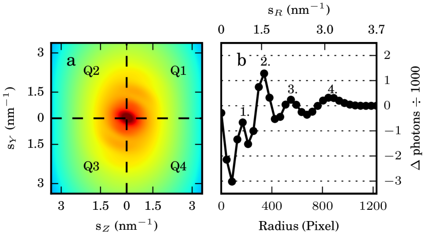
Figure 3: (a) Sum of the calculated diffraction paterns of helium, Fig. 2 c, and the strongly aligned 2,5-diiodothiophene molecules, Fig. 2 b; the color scale is the same as in Fig. 2 . (b) Radial differences $\Delta\mathrm{q}$ between the quadrants Q1–Q4 extracted from (a). Non-zero values result from correspondingly anisotropic features in the diffraction patterns, which originate solely from the aligned molecular diffraction pattern; see text for detail. The locations of the first four maxima of the I–I interference fringes are highlighted by the numbers 1–4; see text for details.

The expected diffraction pattern, i. e., the sum of Fig. 2 b,c, is shown in Fig. 3 a with the same color scale as shown in Fig. 2 . The contrast of the diffraction pattern is strongly reduced due to the contribution from the helium-seed-gas scattering, but the general features are still visible. The contribution of the seed-gas scattering and isotropic background from rest gas in the chamber can be removed as described in the following procedure: Q1…Q4 represent the different quadrants of the detector, see Fig. 3 a. Even with the x-ray-polarization factor included, the diffraction pattern of atoms or isotropic molecules is symmetric with respect to $Y$ and $Z$, i. e., $\text{Q1(s}_{Y},\text{s}_{Z})=\text{Q2(s}_{Y},-\text{s}_{Z})=\text{Q3(-s}_{Y},-\text{s}_{Z})=\text{Q4(-s}_{Y},\text{s}_{Z})$. Due to the 3D alignment of the molecules at $\alpha\neq{}n\cdot 90\,^{\circ},n=0,1,2\ldots$, the molecular diffraction pattern obeys the symmetries $\text{Q1(s}_{Y},\text{s}_{Z})=\text{Q3(-s}_{Y},-\text{s}_{Z})\neq\text{Q2(s}_{Y},-\text{s}_{Z})=\text{Q4(-s}_{Y},\text{s}_{Z})$. Therefore, the radial distributions $\text{s}_{R}$ for the quadrants, labeled as q₁…q₄, obey the symmetries $\mathrm{q_{1}(s}_{R})=\mathrm{q_{2}(s}_{R})=\mathrm{q_{3}(s}_{R})=\mathrm{q_{4}(s}_{R})$ for the diffraction off atoms and isotropic molecules, and $\mathrm{q_{1}(s}_{R})=\mathrm{q_{3}(s}_{R})\neq\mathrm{q_{2}(s}_{R})=\mathrm{q_{4}(s}_{R})$ for the aligned molecules.

Calculating $\Delta\mathrm{q=(q_{1}+q_{3})-(q_{2}+q_{4})}$ for the simulated diffraction pattern shown in Fig. 3 a results in a radial distribution solely dependent on the summed molecular diffraction patterns, which is shown in Fig. 3 b. Here, the first four maxima of the I–I interference term, highlighted by the numbers 1–4, are visible. The fringes are clearly visible with a strong contrast over the background. The location of the maxima along this radial diffraction pattern mainly depend on the molecular structure, whereas their relative amplitudes are dependent on the DOA and $\alpha$. The spacing of the fringes changes with the radius due to the projection of the Ewald sphere onto the planar detector.

This data shown in Fig. 3 b looks similar to the so-called modified scattering intensity $sM(s)$, which is frequently used in the data analysis of, e. g., gas-phase electron-scattering experiments. However, the approach used here intrinsically suppresses isotropic features in the diffraction pattern, and is, therefore, only applicable to single- or aligned-molecule ensembles, and not applicable to the diffraction of isotropically oriented molecules.

IV Results and discussion

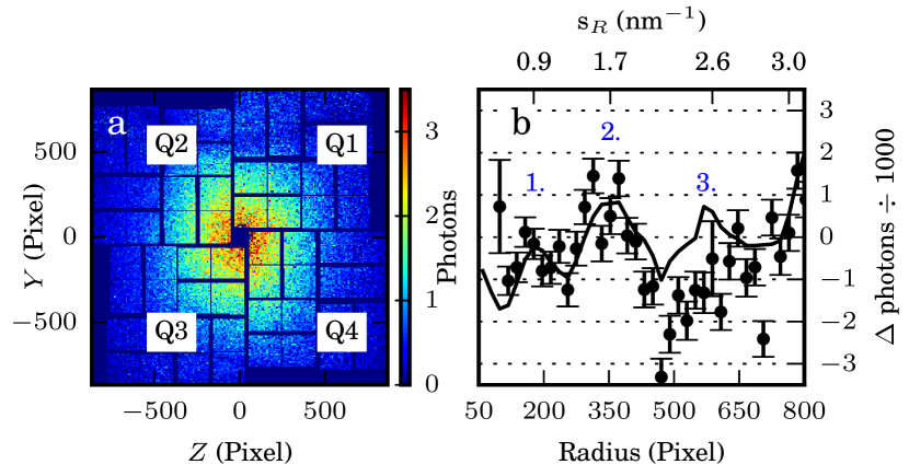
Figure 4: (a) Experimental background-corrected diffraction pattern recorded with the CSPAD camera; the horizontal and vertical dark stripes are due to gaps in the detector. Quadrants are labeled by Q1–Q4, see text for details. (b) $\Delta\text{q}_{\text{norm}}$ for the simulated (solid) and measured (dots with error bars) diffraction pattern. The locations of the first three maxima of the iodine-iodine interference are labeled 1–3.

Fig. 4 a shows the measured diffraction pattern for aligned 2,5-diiodothiophene molecules seeded in helium. For this image $\mathord{\sim}2.2\times 10^{6}$ individual diffraction images have been integrated and background corrected to compensate for photons originating from the beamline, which contributed $\mathord{\sim}30~{}\%$ to the detected number of photons. The background correction was performed by subtracting averaged images from measurements without molecular beam, i. e., the molecular beam was either switched off or temporally delayed such that the XFEL pulses missed it. This resulted in the diffraction pattern shown in Fig. 4 a. For illustration purposes, the recorded diffraction was averaged between neighboring pixels over a $7\times 8$ pixel window, resulting in a 2D diffraction pattern with decreased pixel-based fluctuations and largely avoided negative intensities resulting from the background correction. The horizontal and vertical dark stripes in the image are due to gaps in the CSPAD detector, c. f. Fig. 1 . Q1…Q4 label the different quadrants of the detector as in Fig. 3 a.

Fig. 4 b shows the radial difference between the quadrants, $\Delta\text{q}_{\text{norm}}$ for the simulation (solid line) and the experiment (points), c. f. Fig. 3 b. Unlike $\Delta\text{q}$, $\Delta\text{q}_{\text{norm}}$ contains a radius-dependent correction factor accounting for the lower number of summed pixels per bin due to the gaps of the detector. The error bars for the experimental data are given as one standard deviation; we note that they are largely independent of radius due to the distribution of beamline-scatter background with most intensity on the outer part of the detectors, which practically cancels the expected noise-distribution from the signal itself. The simulated diffraction pattern was modified by the gaps of the detector before $\Delta\text{q}_{\text{norm}}$ was calculated.

The simulations show that the first three maxima of the I–I interference are clearly visible despite of the gaps; the fourth maximum is already strongly influenced by missing pixels and, therefore, is not shown any more. For radii $\lesssim 100$ pixel ($\text{s}_{R}<0.04$) the measured signal strongly deviates from the simulations, with ordinate values higher or lower than the shown range. This is attributed to stray photons from the direct x-ray beam, which are strongly observable close to the central hole of the detector.

The first two maxima of the I–I interference pattern – and hence the first maximum of the I–S interference – are matched well by the measurement, including a change of sign around the second maximum. At higher scattering angles the deviation between measurement and simulations is increasing. Here, the intensities in the measurement are overall smaller than in the simulation, but the general trend of an increased signal around the third maximum is comparable. The deviation is assigned to the small diffraction signal for scattering angles $s_{R}>0.2$, which leads to an larger influence of the measured background photons.

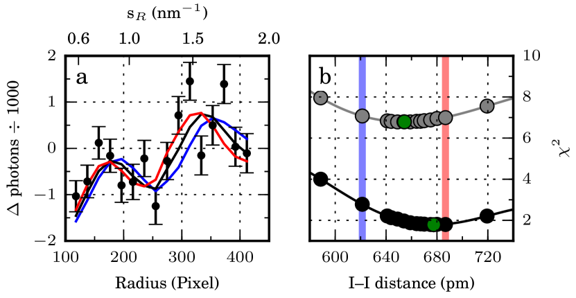
Figure 5: (a) $\Delta\text{q}_{\text{norm}}$ for the first two maxima of the diffraction pattern. The solid lines show the simulated diffraction pattern for the calculated I–I bond distance (black), and a varying bond distances in a range +/- 5 %, i. e., 686.7 and 621.3 pm (red, blue). See Fig. 4 for the comparison between experiment and simulation over the full radial range. (b) Reduced chi-square value (points) in dependence of different simulated I–I bond distances for two scattering ranges $\mathrm{s_{R1}}$ (black, same as (a)), and $\mathrm{s_{R2}}$. Polynomial fits (solid) were used to determine the respective minima, which are highlighted by the green points. As in (a), the vertical red and blue lines show the +/- 5 % range from the calculated bond distance.

The I–I bond length is reconstructed from the experiment by a comparison to several simulated molecular diffraction patterns with varying I–I bond distance. In Fig. 5 a the experimental data are compared to simulated $\Delta\text{q}_{\text{norm}}$ for three different I–I bond distances, namely the computed equilibrium distance of 654 pm (black), vide supra, and for a variance of $\pm 5$ % of the I–I bond (red/blue). The I–I distances were varied by symmetrically elongating the iodines along the connecting line while keeping the rest of the molecular structure unchanged. By focusing on the scattering range $\mathrm{s_{R,1}}=[0.58,2]~{}\text{nm}^{-1}$, which contains the first two maxima of the I–I interference pattern, the simulations already show that changes on the order of $\pm 5$ % in distance shift the radial maxima inevitably toward higher and lower scattering angles, respectively.

In order to quantitatively determine the best-fit I–I distance for the experimental data, we performed a $\chi^{2}$ analysis of the simulations against the experimental data. The black points in Fig. 5 b show the reduced $\chi^{2}$ values  for different I–I distances for the scattering range $\mathrm{s_{R1}}$; the gray points show the same analysis for a scattering range of $\mathrm{s_{R,2}}=[0.58,3.13]~{}\mathrm{nm^{-1}}$, which includes the third maxima of the I–I interference pattern. The corresponding solid lines show polynomial fits to the $\chi^{2}$-values. The fits provide an optimized bond distance of $677$ pm and $654$ pm for the scattering ranges $\mathrm{s_{R,1}}$ and $\mathrm{s_{R,2}}$ with corresponding $\chi^{2}$ values of $1.8$ and $6.8$, respectively. Both minima are highlighted by an additional green point. The retrieved distances are in very good agreement with the quantum-chemistry distance of 654 pm, and are clearly within $\pm 5$ % of the calculated I–I distance, indicated by the vertical red (blue) line.

V Summary and outlook

We presented experimental results on the diffractive imaging of controlled gas-phase molecules. The molecules were strongly aligned by an in-house TSL, which allowed the measurement of diffraction patterns at the full LCLS repetition rate Kierspel et al. (2015) of 120 Hz. The aligned molecules were probed with hard x-ray photons at a photon energy of 9.5 keV. The molecular diffraction pattern of a 3D-aligned molecular ensemble was successfully extracted, as confirmed by utilizing the different symmetries in the diffraction pattern of the aligned molecules and the seed gas. The extracted iodine-iodine distance was in agreement with the calculated molecular structure to within a few percent.

We note that this iodine-iodine distance in the static molecule could also have been measured using gas electron diffraction or x-ray scattering off a dense isotropic gas. However, the current experimental demonstration of this measurement using aligned molecules and femtosecond pulses of hard x-rays provides crucial steps toward the coherent diffractive imaging of ultrafast molecular dynamics at the atomic scale, the long-sought after “molecular movie”: Conceptionally, the aligned molecules Stapelfeldt and Seideman (2003); Holmegaard et al. (2010); Kierspel et al. (2015); Trippel et al. (2018b); Owens, Yachmenev, and Küpper (2018) enable the recording of the three-dimensional coherent diffraction image of the molecule instead of a one-dimensional radial scattering distribution, i. e., in principle, it provides information on the three-dimensional structure of molecules instead of the pair-distribution functions obtained from standard electron or x-ray scattering. The femtosecond x-ray pulses provide the means to follow ultrafast dynamics with atomic resolution.

In a previous experiment Küpper et al. (2014), 1D aligned molecules were probed at a much lower photon energy (2 keV, $\lambda_{\text{{XFEL}}}=~{}600~{}\text{pm}$), which led to a resolvable structure in the order of the size of the molecule. The larger photon energy in the current experiment allowed for the quite precise measurement of an intramolecular atomic distance, albeit so far with a decreased signal-to-noise ratio (SNR) due to the lower coherent scattering cross section, higher incoherent scattering cross sections, and a reduced photon flux from the LCLS facility. The SNR, largely limited by large background contributions from the beamline and the last x-ray aperture before the interaction region, was really the limiting factor in this experiment as, for example, the obtained 2D diffraction pattern of the static structure of 2,5-diiodothiophene shown in Fig. 4 a is very noisy. A comparison between experiment and simulation was only useful by improving the SNR in the data analysis by summing up neighboring pixels, and calculating differential radial plots as shown in Fig. 4 b.

Based on our simulations we estimate that for this measurement the difference between the diffraction pattern of 1D and 3D aligned 2,5-diiodothiophene molecules would be negligible. However, we further estimate that the number of acquired individual diffraction patterns was sufficient to distinguish between 1D and 3D-aligned molecular ensembles if the molecular degree of alignment was close to 1, hinting at the possibility to determine the complete molecular structure.

The experimental setup was technically capable of investigating ultrafast molecular dynamics: The setup provided a collinearly aligned femtosecond laser pulse, which was powerful enough to dissociate the aligned molecules Kierspel et al. (2015). But the measurement of molecular dynamics requires a higher number of scattered photons or an improved SNR.

Experimentally, the SNR can be improved by reducing the number of background photons on the detector via, for example, optimized x-ray apertures, or by the implementation of the electric deflector Chang et al. (2015); Trippel et al. (2018a) into the experimental setup. The deflector is placed between the valve and the interaction zone, and allows to spatially separate polar molecules from the seeding gas. This technique was applied once for the diffractive imaging of controlled molecules Küpper et al. (2014); Stern et al. (2014), but was not applied here due to the corresponding longer distance from valve to interaction point, resulting in a lower density of the molecular beam.

The repetition rates of the recently launched European XFEL or the upcoming LCLS II are a few hundred to a few thousand times higher than available here and these facilities will provide a near-infrared laser synchronized with the XFEL, which will align molecules at very high repetition rates Trippel et al. (2013); Kierspel et al. (2015); alternatively, continuous-wave alignment could be exploited Deppe et al. (2015). If the molecular alignment is achieved at the full repetition rates of these upcoming facilities, the presented experiment results can be measured within two minutes at the European XFEL or a few seconds at the LCLS II. Such experimental parameters provide a feasible start for the recording of ultrafast molecular dynamics of small 3D-aligned gas-phase molecules Barty, Küpper, and Chapman (2013), or to image small biomolecules without heavy atoms in the molecular frame.