art,methReferences,Referencesnaturemag naturemag

A 100-kiloparsec galactic wind feeding the circumgalactic medium of a massive compact galaxy

Abstract

Ninety per cent of baryons are located outside galaxies, either in the circumgalactic or intergalactic medium2012ApJ…759…23S,2017ARA&A..55..389T. Theory points to galactic winds as the primary source of the enriched and massive circumgalactic medium 2011Sci…334..948T,2014ApJ…792….8W,2013MNRAS.430.1548H,2013MNRAS.432…89F. Winds from compact starbursts have been observed to flow to distances somewhat greater than ten kiloparsecs2014Natur.516…68G,2016ApJ…820…48Y,2017Natur.548..430F,2018ApJ…864L…1G, but the circumgalactic medium typically extends beyond a hundred kiloparsecs2011Sci…334..948T,2014ApJ…792….8W. Here we report optical integral field observations of the massive but compact galaxy SDSS J211824.06$+$001729.4. The oxygen [O 2] lines at wavelengths of 3726 and 3729 angstroms reveal an ionized outflow spanning 80 by 100 square kiloparsecs, depositing metal-enriched gas at 10,000 kelvin through an hourglass-shaped nebula that resembles an evacuated and limb-brightened bipolar bubble. We also observe neutral gas phases at temperatures of less than 10,000 kelvin reaching distances of 20 kiloparsecs and velocities of around 1,500 kilometres per second. This multi-phase outflow is probably driven by bursts of star formation, consistent with theory2018MNRAS.481.1873L,2018MNRAS.475.1160H.

Department of Physics, Rhodes College, Memphis, TN, USA; drupke@gmail.com

Center for Astrophysics & Space Sciences, University of California, San Diego, La Jolla, CA, USA

Centre for Astrophysics Research, School of Physics, Astronomy & Mathematics, University of Hertfordshire, Hatfield, UK

Department of Astronomy, University of Wisconsin-Madison, Madison, WI, USA

Department of Physics and Astronomy, Bates College, Lewiston, ME, USA

Department of Physics and Astronomy, Dartmouth College, Hanover, NH, USA

National Radio Astronomy Observatory, Charlottesville, VA, USA

Department of Physics and Astronomy, Siena College, Loudonville, NY, USA

Department of Physics and Astronomy, University of Kansas, Lawrence, KS, USA

Department of Astronomy, University of Florida, Gainesville, FL, USA

University of Crete, Heraklion, Crete, Greece

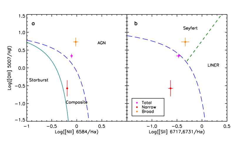
Figure 1: Line ratio diagrams of the core spectrum. In a, the green solid line demarcates the edge of the $z=0$ pure star-formation locus2003MNRAS.346.1055K; in both panels, blue long-dashed lines denote the limits of young star photo-ionization2006MNRAS.372..961K; and in b, the green short-dashed line separates Seyfert galaxies (AGNs) from low-ionization nuclear emission-line regions (LINERs)2006MNRAS.372..961K. Error bars are 1$\sigma$. The red narrow component is consistent with star formation at near-solar metallicity, while the broad, outflowing component is ionized by either an AGN or high-velocity shocks.

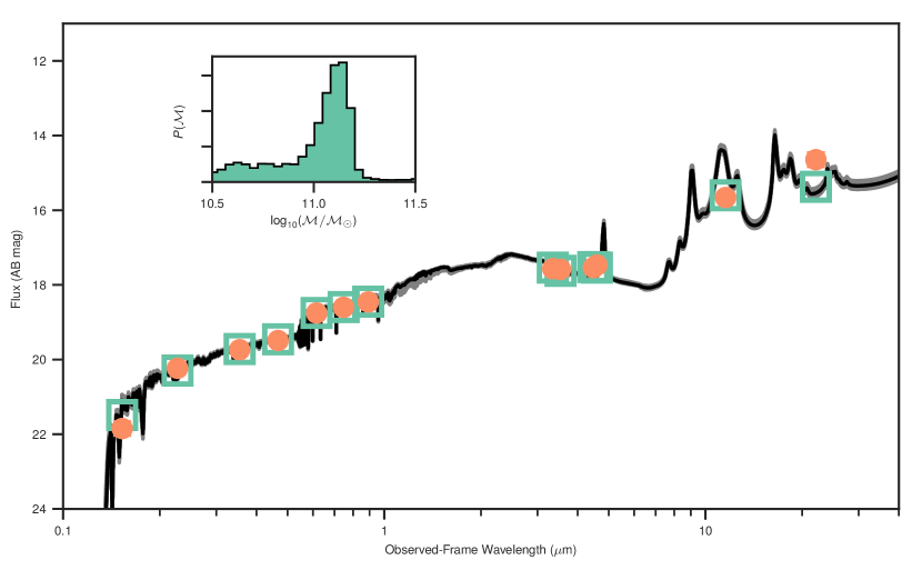
Figure 4: Fit to the ultraviolet-to-mid-infrared spectral energy distribution. The best-fit model and 1$\sigma$ error are shown as a black line and grey shading; observed fluxes with 1$\sigma$ errors (usually smaller than the symbols) are yellow circles; and model fluxes are open cyan boxes. Flux is given in AB magnitudes and observed-frame wavelengths in micrometres. The posterior probability $P(M)$ for stellar mass $M$ is shown in the inset.

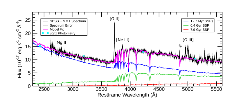
Figure 5: Stellar population model fit. Spectral data from SDSS and the MMT and 1$\sigma$ errors are shown as the black line and grey shading. SDSS $ugriz$ photometry and 1$\sigma$ errors are the cyan squares and grey vertical bars. The best-fit model is a magneta line; the stellar population components summed to produce this model are shown as coloured lines, with ages as shown. SSP, simple stellar population.

The galaxy J211824.06$+$001729.4 that we study here, which we call Makani (Hawai’ian for ‘wind’), is an example of a merger of two galaxies hosting a galactic wind thought to be powered by extreme star-formation surface density2012ApJ…755L..26D. At redshift $z=0.459$, Makani is a compact but massive galaxy, with log$(M_{\star}/M_{\odot})=11.1(\pm 0.2$), where $M_{\star}$ and $M_{\odot}$ are the stellar and solar masses, respectively (Extended Data Fig. 4). Our Hubble Space Telescope imaging analysis reveals a highly peaked stellar core (radius 400 pc) framed by two tidal tails of 10–15 kpc so that half of the galaxy’s light extends to about 2.5 kpc (ref. 2014MNRAS.441.3417S; Fig. 1). Its stellar populations include old (more than a billion years, Gyr), medium-aged (0.4 Gyr), and young ($<$7 million years, Myr) components (Extended Data Fig. 5), with a current star-formation rate of 100–200M_⊙ yr^-1. It may contain a dust-obscured accreting supermassive black hole, or active galactic nucleus (AGN), on the basis of its X-ray luminosity of log$L(2-10\,\mathrm{keV})=42.5^{+0.4}_{-0.6}$ erg s^-1 (ref. 2014MNRAS.441.3417S), its mid-infrared slope, and the presence of highly ionized gas like [Ne 5] at wavelength $\lambda=3426$ Å (log$L=40.6^{+0.1}_{-0.2}$ erg s^-1). However, any AGN is not currently energetically dominant2012ApJ…755L..26D,2014MNRAS.441.3417S or radio-loud (G. C. Petter et al., manuscript in preparation) and the data could be explained by star formation and shocks. Extremely high-density star formation, like that found in Makani, is capable of powering fast winds, independent of an AGN2012ApJ…755L..26D.

To study the spatial extent of its outflow, we observed Makani with the Keck Cosmic Web Imager (KCWI)2018ApJ…864…93M. The emission from the [O 2] lines at $\lambda=3726$ Å and 3729 Å in these data reveals a nebula with approximate mirror symmetry around the north-south and east-west axes, extending to radii of 50 kpc north and south of the galaxy nucleus, and 40 kpc east and west (Fig. 1). Its morphology resembles that of a limb-brightened, bipolar bubble, similar to those seen in other galactic winds1998ApJ…493..129S,2015ApJ…800…45H but on a much larger scale. This nebula is remarkable in the context of other [O 2] emitters. Its area of 4,900 kpc² (136 arcsec² above a 5$\sigma$ surface brightness limit per spaxel (spectral pixel) of 5$\times$10^-18 erg s^-1 cm^-2 arcsec^-2) makes it the largest [O 2] nebula detected around a single galaxy in the field2015ApJ…799..205B, 2017ApJ…841…93Y or in galaxy groups2018AA…609A..40E,2018ApJ…869L…1J. Its [O 2] luminosity of 3.3$\times$10⁴² erg s^-1 is several times the break in the galaxy luminosity function, $L_{*}$, at $z\approx 0.45$ (ref. 2009ApJ…701…86Z). Its rest-frame equivalent width (40 Å), half-light radius (17 kpc), and maximum radial extent (50 kpc) put it at the top end of [O 2] emitters at $z\leq 0.6$ and radio galaxy nebulae2015ApJ…799..205B,2012MNRAS.427.2401K, perhaps indicative of the unusual nature of this nebula as a giant galactic wind.

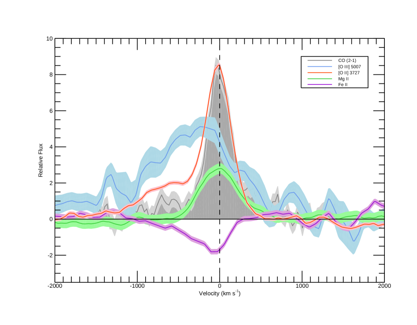
Figure 2: Comparison of velocity profiles among gas phases. Tracers are shown as coloured lines, while the CO(2–1) profile is shaded in grey. The data are smoothed by thjree pixels and the coloured shadings indicate 1$\sigma$ errors on the line fluxes. The ultraviolet-optical nebular lines are shown with the correct relative fluxes (uncorrected for reddening in the host galaxy), while the CO(2-1) line is arbitrarily scaled. The spatially integrated velocity profiles probe different gas phases and spatial scales but show remarkable overall consistency.

Based on its light distribution alone, the hourglass shape of the nebula strongly suggests a bipolar galactic wind emerging from its host galaxy. The spatially-resolved gas kinematics confirm this impression and separate the wind cleanly into an outer region with low-velocity gas only and an inner region containing both low- and high-velocity gas (Fig. 2). The outer region with lower velocities spans radii 20–50 kpc, while the high-velocity gas is concentrated within a radius of about 10 kpc. We call these two wind components, and the associated starbursts that are thought to have produced them, episodes I (0.4 Gyr ago) and II (7 Myr ago). We sort spaxels by the average maximum blueshifted velocity of $\langle v_{98\%}\rangle=-700$ km s^-1, though sorting by velocity dispersion $\sigma$ produces similar results. Episode I then has gas with maximum blueshifted velocities between $-100$ and $-700$ km s^-1 while episode II has a high-velocity tail of gas to $v_{98\%}=-2,100$ km s^-1. Timescale arguments further support the existence of two starburst-driven wind episodes. In the 0.4 Gyr since the episode I starburst, a constant-velocity wind must have travelled at 120 km s^-1 to reach the edge of the nebula (50 kpc); representative velocities at the nebula outskirts are in fact 100–200 km s^-1. In the 7 Myr since the most recent starburst episode began, the speed required to reach the edge of the bulk of the episode II wind (10 kpc) is 1,400 km s^-1, which is also a typical maximum velocity in the inner nebula. The lack of high-velocity redshifted gas in episode II may be due to dust in the outflow blocking the far side of the wind, while the lack of high-velocity gas in the episode I wind is probably due to the dispersal of high-velocity gas to radii exceeding 50 kpc over 0.4 Gyr or the deceleration of the outflow as predicted by models2018MNRAS.481.1873L. Episode I gas also forms the telltale hourglass shape and has higher typical velocity dispersions (200 km s^-1) than expected for tidal features or gravitational motions at large radii 2018AA…618A..94P.

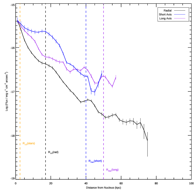
Figure 3: [O 2] spatial profiles. Profiles are averaged and then plotted versus distance from the galaxy nucleus along circular radii (black); the short axis of the nebula, or east-to-west axis (blue); and the long axis of the nebula, or north-to-south axis (purple). The averages are taken in directions perpendicular to these: in azimuth around the nucleus; along the long axis; and along the short axis, respectively. The short and long axis profiles are shifted upward in flux so that the three profiles match in the lowest distance bin. Errors are standard errors of the mean. Plotted as dashed lines are the stellar half-light radius (orange), the [O 2] half-light radius within 50 kpc (black), and the [O 2] maximum radius along the short and long axes (blue and purple).

We find two other gas phases that we associate with the episode II (recent, inner) outflow. Using the Atacama Large Millimeter Array (ALMA), we detect molecular gas traced by CO(2–1) emission that is outflowing in a compact form, both blueshifted at -500 to -1,500 km s^-1and redshifted at 500–1,500 km s^-1, from the nucleus 10 kpc northward (Fig. 3d). This gas is clearly part of episode II, given its high velocity and compact scale. Lower-velocity molecular gas, at $|v|<500\,\mathrm{km\,s^{-1}}$ and radius $r<20$ kpc (Fig. 3c), is also likely to be part of the outflow because it is much more extended than the stellar disk and correlates spatially with extended, outflowing ionized gas. It may be gas from episode II that has decelerated after reaching scales of the order of 10 kpc. Using resonant line emission from Mg 2 at $\lambda=2796$ Å and 2803 Å, we also detect neutral gas of temperature $T\approx 10^{4}$ K in the velocity range $\pm$500 km s^-1 (Fig. 3b). This emission correlates with some regions of faint, extended CO and [O 2] emission. Although these velocities are modest, resonant emission on 10-kpc scales has so far been detected only in galactic winds, and because of strong radiation transfer effects such emission is not highly shifted from the redshift of the Makani galaxy’s centre of mass2011ApJ…728…55R,2011ApJ…734…24P. Blueshifted Fe 2 absorption is detected in the nuclear spectrum (Extended Data Fig. 2), but tracing its physical extent requires deeper observations.

Estimates of the mass contained within the wind would complete its portrait. However, the mass of the ionized gas is uncertain without spatially resolved recombination line measurements. Bootstrapping from single-aperture H$\alpha$ and H$\beta$ measurements, we estimate $6(^{+6}_{-3})\times 10^{8}(200\,\mathrm{cm}^{-3}/\mathrm{n_{e}})$$M_{\odot}$ of ionized gas in the nebula, with unquantified systematic errors (electron density $n_{e}$ and ionization state) likely exceeding the measurement error. Although it is confined to the inner 10 kpc, the mass of the molecular gas in the $|v|=500\text{--}1500$ km s^-1 flow (that is, episode II) is substantial ($2.4^{+0.6}_{-0.6}\times 10^{9}$$M_{\odot}$), with four times as much in the more extended $\pm$500 km s^-1 component. The ionized gas plus molecular wind thus contains 1–10% of the galaxy’s baryonic mass, a fraction that will be even larger when all phases are accounted for. The resulting mass flow rate for the molecular episode II component is $dM/dt\approx Mv/r=245$M_⊙ yr^-1 for $v=1,000$ km s^-1 and $r=10$ kpc, which is roughly one to two times the star-formation rate. This is consistent with molecular outflow rates2014Natur.516…68G,2018ApJ…864L…1G from other compact starburst mergers at $z>0.5$.

The huge, metal-enriched outflows in Makani – a key component of the host galaxy’s dynamically and chemically evolving circumgalactic medium (CGM) – are consistent with the types of star-formation or AGN-driven winds that populate and enrich the CGM in theoretical models2018MNRAS.481.1873L,2018MNRAS.475.1160H. A model galaxy forming stars at 100M_⊙ yr^-1 in a baryonic halo of $2\times 10^{11}$$M_{\odot}$ and supernova-driven winds propelling gas with initial velocity 1,000 km s^-1 produce a 10⁹$M_{\odot}$ (or 10¹⁰$M_{\odot}$) shell at $r\approx 10$ kpc (or 100 kpc) in $t\approx 10$ Myr (or 400 Myr), with velocities at this time of order 1,000 km s^-1 (100 km s^-1)2018MNRAS.481.1873L. These numbers bear a striking resemblance to the observations in the context of the two-episode outflow we propose. The wind will continue to expand, diffuse, and virialize over longer timescales, as this nebula is denser and more structured than virialized CGM gas2014ApJ…792….8W,2018MNRAS.475.1160H and has reached perhaps only about 10% of the virial radius2010ApJ…717..379B of a log$(M_{\star}/M_{\odot})=11.1$ galaxy at $z=0.46$.

The size of this wind makes it the one of the largest wide-angle, galaxy-scale outflows yet observed, with scales much larger than in other compact or high-$z$ starbursts2014Natur.516…68G,2018ApJ…864L…1G,2017Natur.548..430F. The morphology and velocity of the wind in the Teacup AGN make it a cousin of Makani, but on scales five to ten times smaller2015ApJ…800…45H. Though the Teacup also hosts diffuse gas over 100 kpc scales, this gas has a different physical origin than does the gas in Makani2018MNRAS.474.2302V. The most comparable system may be a merger with compact star formation at a cosmic distance ten times closer than Makani. NGC 6240 ($z=0.04$) has an ionized outflow that reaches a 40-kpc radius2016ApJ…820…48Y. However, the outflow size relative to the stellar half-light radius (inside which half of the galaxy’s starlight resides) is only $r/r_{*,1/2}\approx 4$ in NGC 6240 (ref. 2013ApJ…768..102K), versus $r/r_{*,1/2}>20$ in Makani, and much of the NGC 6240 nebula coincides with stellar tidal features, unlike Makani. Furthermore, the H$\alpha$ luminosity of the NGC 6240 nebula is four times smaller than in Makani if the core H$\alpha$ emission follows the oxygen emission at a constant [O 2]/H$\alpha$ line ratio.

With a maximum extent of more than twenty times the stellar half-light radius, the oxygen nebula observed here has propagated well into the galaxy halo, placing it solidly in the CGM. The cool gas and metals in the flow are thus contributing to the buildup and enrichment of the CGM. This cool gas can be propelled by hot gas, radiation pressure or cosmic rays. The classic model of hot gas acceleration faces the problem that cold clouds may be destroyed during acceleration. These clouds may simply reform after being shredded and mixed in the hot wind2016MNRAS.455.1830T or the clouds may survive the acceleration through fast radiative cooling2018MNRAS.480L.111G. The mixing layers in shredded clouds can also cool hot gas from the halo or CGM, enhancing the amount of cool gas injected into the CGM2018MNRAS.480L.111G. If the cool outflow is accelerated by a hot wind, the existence of [O 2]-emitting gas at all radii argues for either cloud reformation on very short timescales or for cloud survival (coupled with enhancement from hot gas). The outflow we observe is thus feeding the CGM by directly depositing gas from the galaxy or by entraining and cooling hot halo and circumgalactic gas.

Connecting the CGM with ongoing galactic winds has been challenging because of the lack of clear evidence for such winds on large enough scales. Previous evidence came from theory2013MNRAS.430.1548H,2013MNRAS.432…89F and the statistical characteristics of the CGM as measured from single quasar absorption lines over large galaxy populations2011Sci…334..948T,2014ApJ…792….8W. We have now observed a single galaxy, with all lines of sight accounted for, whose wind has entered the CGM. Our measurement provides one of the first direct windows into the dynamically and chemically evolving, multiphase CGM being created around a massive galaxy.

hizeaj2118

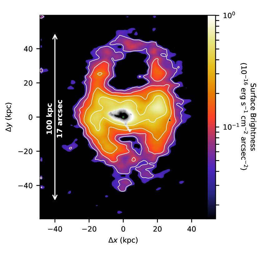
Figure 1: The giant galactic wind surrounding the massive, compact galaxy Makani, observed by emission from the [O 2] line at $\lambda$=3726 Å and 3729 Å. The colour scale and white contours show observed-frame surface brightness, and the axes are labeled in kiloparsecs from the galaxy nucleus. Contours are 2–16% of peak flux, spaced by factors of 2. A rest-frame $V$-band image of the galaxy (Hubble Space Telescope/WFC3 F814W filter) is superimposed on the center of the [O 2] image taken with KCWI at the Keck II telescope. The small circle at the centre illustrates the radius of the compact core (400 pc). North is up and east is to the left.

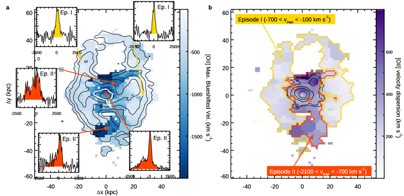
Figure 2: Velocity maps of the galactic wind. The velocities are from fits to Voronoi-binned [O 2] data and are calculated from the red side of the cumulative velocity distribution function to specified percentiles as maximum blueshifted velocity $v_{\mathrm{max}}\equiv v_{98\%}=v_{50\%}-2\sigma$ (a) and velocity dispersion $\sigma\equiv(v_{34\%}-v_{68\%})/2$ (b). In a, the blue colour denotes velocity. The insets show the deblended and stacked [O 2] doublet versus velocity; these highlight representative bins for each star formation or outflow episode. The black line is the continuum-subtracted spectrum, and the yellow or red filled profile is the emission line model. The colour denotes whether the spaxel is part of episode I (yellow) or episode II (red). The black contours are as in Fig. 1, and the white Hubble Space Telescope contour represents 1% of the peak stellar continuum flux, accentuating the extended diffuse stellar emission from tidal forces in the merger. In b, the purple colour denotes velocity dispersion and the yellow and red contours outline regions of specified $v_{\mathrm{max}}=v_{98\%}$ to delineate episodes I and II. The spatial separation of the episodes is also reflected in the $\sigma$ map. The black contours in b outline the inner concentration of ionized gas at velocities $-1,500$ to $-500$ km s^-1 (Fig. 3d). We securely detect high-velocity [O 2] beyond this inner region through Voronoi binning.

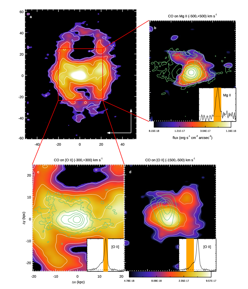
Figure 3: Comparison of the ionized, neutral atomic and molecular phases of the galactic winds. The [O 2] map from Fig. 1 is replicated in a, with the north and east directions indicated in the lower right. In b, a zoomed-in view of the inner 40 kpc, molecular gas in restored CO(2–1) (green contours) is plotted on top of Mg 2 emission (colour, with white contours) in the same velocity range ($-$500 to $+$500 km s^-1). Panel c compares the low-velocity molecular (restored CO, green contours) and ionized gas ([O 2], colour and white contours) over the same velocities ($-$300 to $+$300 km s^-1). The CO contours are 0.09, 0.14, 0.28, 0.5, 0.8 and 1.2 mJy per beam. Panel d is the high-velocity molecular gas (tapered, bottom right, contours of 0.08, 0.11, 0.122, 0.132, and 0.14 mJy per beam) on an [O 2] channel map showing the brightest regions of high-velocity ionized gas, both over $-$1,500 to $-$500 km s^-1. In each zoom box, the inset spectrum is a plot of spatially integrated optical line flux versus velocity ($-$2,500 to $+$2,500 km s^-1), with the linemap velocity range highlighted in orange.

0.1 KCWI observations and data analysis.

SDSS J211824.06$+$001729.4 was originally selected as an intermediate-redshift starburst galaxy with broad but spatially unresolved line emission2012ApJ…755L..26D,2014MNRAS.441.3417S, part of a population known to host strong outflows2007ApJ…663L..77T. We observed it with KCWI on the Keck II telescope on 6 November 2018 UT (Universal Time) for 40 min. We employed the blue low-dispersion (BL) grating and medium slicer with KCWI, yielding a resolution of 2.5 Å and wavelength coverage of 3435–5525 Å. We chose a central wavelength of 4500 Å and detector binning of 2$\times$2. Conditions were photometric, with 0.6^′′ seeing. Two exposures were dithered 0.35^′′ along slices to subsample the long spatial dimension of the output spaxels (0.69^′′$\times$0.29^′′). The field of view of the reduced data cube is 15.4^′′$\times$19.4^′′.

We reduced the data using the KCWI data reduction pipeline and the IFSRED library2014ascl.soft09004R. As the default scattered light subtraction in the pipeline leaves visible residuals, we use a routine (IFSR_KCWISCATSUB) to subtract scattered light by summing the data in 100-pixel increments along columns (parallel to the dispersion direction) and fitting the least contaminated inter-slice regions along rows (parallel to the spatial direction) with low-order polynomials. The default wavelength calibration also produces large root-mean-square (r.m.s.) residuals because of a mismatch with the pipeline thorium-argon (ThAr) atlas, so we extract a representative spectrum from our data and find its wavelength solution using IDENTIFY in PyRAF (www.stsci.edu/institute/software_hardware/pyraf). 16/20 lines in the 3500–4000 Å and 5000–5600 Å ranges are from Th; the other 38 lines (including most of the brightest lines) are from Ar. The resulting r.m.s. residual is 0.18 Å. We then input this calibrated spectrum as the atlas into the pipeline, yielding a 0.07 Å r.m.s.. Following the pipeline stages, we resample the data (IFSR_KCWIRESAMPLE) onto a 0.29^′′$\times$0.29^′′ spaxel grid; align the two exposures by fitting the galaxy centroid (IFSR_PEAK); and mosaic the data (IFSR_MOSAIC). The resulting stacked and resampled field of view at 5000 Å is 53$\times$67 spaxels. The reconstructed KCWI continuum image (rest-frame near-ultraviolet) is consistent with the Hubble Space Telescope WFC3/F814W image (rest-frame $V$) when convolved with a 15-pixel Gaussian kernel to match the measured seeing. Finally, we sum the nebula’s core emission in a 3.0^′′ circular aperture to match the Sloan Digital Sky Survey (SDSS)2000AJ….120.1579Y spectrum.

We created initial [O 2] linemaps by integrating over [O 2] and subtracting nearby continuum windows on either side. The wavelength interval of each map is calculated from the doublet average wavelength at a given velocity. We then used $\pm$300 km s^-1 flux and error maps to create Voronoi bins (where the velocity applies to the centroid of the [O 2] doublet; the doublet lines are 2.6 Å apart, which corresponds to 200 km s^-1). The IDL (www.harrisgeospatial.com/Software-Technology/IDL) routine VORONOI_2D_BINNING2003MNRAS.342..345C is used to construct the bins, with a target signal-to-noise ratio of 10 and a threshold signal-to-noise ratio of 1. We fit the core spectrum, the full data cube, and the Voronoi binned data cube with IFSFIT2014ascl.soft09005R. Because very few strong stellar lines arise in our spectra (rest frame 2350–3790 Å), we use a scaled continuum derived from the fit to the rest-frame 2550–5600 Å spectrum2014MNRAS.441.3417S (see below). We fit two velocity components to the [O 2] and [Ne 5] lines. If any component falls below 2$\sigma$ in a spaxel, the spectrum is re-fit with fewer components. Allowing the [O 2] line ratio to float freely in the narrow component of the core spectrum results in an [O 2]3729 Å/[O 2]3726 Å ratio of 1.2 (corresponding to $\mathrm{n_{e}}\approx 200$ cm^-3), while the broad component ratio is unconstrained. We thus fix the [O 2] ratio to 1.2 in all fits. In the core spectrum, Mg 1 2852 Å, Mg 2 2796, 2803 Å, and Fe 2* 2612, 2626 Å are tied to the same velocity and width and fitted with a single component. The continuum fits to each spaxel are used to subtract the stellar continuum around [O 2] or Mg 2 to produce the linemaps shown in Figs. 1–3. The [O 2] linemaps have a limiting 1$\sigma$ surface brightness per pixel of 1.0$\times 10^{-18}$ erg s^-1 cm^-2 arcsec^-2. For display purposes only, these maps are interpolated to a grid ten times finer and the $\pm$300 km s^-1 maps are clipped at 1.5% of peak flux (or 4$\sigma$).

The core spectrum yields detections of [O 2], [Ne 5] 3426 Å, Mg 1 2852 Å, Mg 2 2796, 2803 Å, and Fe 2* 2612, 2626 Å in emission, and Fe 2 2586 Å in absorption. The emission lines break into two distinct components: a narrow feature at the systemic velocity of the host galaxy ($z=0.45916$; $\sigma=143$ km s^-1 in [O 2], 197 km s^-1 in Mg and Fe emission) and a broad, blueshifted feature that is outflowing ($z=0.45736,~{}v=-540\,\mathrm{km\,s^{-1}},~{}\sigma=500\,\mathrm{km\,s^{-1}}$ in [O 2]; $z=0.45666,~{}v=-750\,\mathrm{km\,s^{-1}},~{}\sigma=392\,\mathrm{km\,s^{-1}}$ in [Ne 5]). We correct upward spatially-integrated line fluxes and luminosities for a Galactic extinction of $A_{V}=0.2075$ (ref. 2011ApJ…737..103S), which corresponds to a 22% correction at [O 2]. We use the 2018 Planck cosmology2018arXiv180706209P to calculate luminosity and angular size distances. The spatially-integrated [O 2] flux is $4.0(\pm 0.2)\times 10^{-15}$ erg s^-1 cm^-2. From the core spectrum we measure a Mg 2 flux of $2.3(\pm 0.1)\times 10^{-16}$ erg s^-1 cm^-2, which corresponds to a rest-frame equivalent width 2.3 Å and a luminosity of $1.5\times 10^{41}$ erg s^-1. The [Ne 5] line flux is $4.3(\pm 1.2)\times 10^{-17}$ erg s^-1 cm^-2.

0.2 Ionized and neutral gas properties.

We parameterize the velocity distribution of the [O 2]-emitting gas in each spaxel using the cumulative velocity distribution function (CVDF). In spaxels where only one component is fitted, this is a Gaussian; for two components, the CVDF is the sum of two independent Gaussians. We use the 50th and 98th percentile of the CVDF ($v_{50\%}$ and $v_{98\%}$, as measured from the red side of the line) to represent the mean and most blueshifted (’maximum’) velocities. We define the width of the CVDF as $\sigma\equiv(v_{34\%}-v_{68\%})/2$, which for a single component is the usual Gaussian $\sigma$.

We combine our KCWI data with two other spectra to constrain the integrated gas excitation, reddening, and gas mass. The first is the SDSS spectrum that, along with [O 2], covers the [Ne 3] 3869 Å, H$\beta$, and [O 3] 4959 Å, 5007 Å emission lines. The second is a spectrum acquired with Keck/NIRSPEC, which covers the H$\alpha$, [N 2] 6548 Å, 6583 Å, and [S 2] 6717 Å, 6731 Å lines. The latter was observed with a 0.76^′′-wide slit at a position angle of 83^∘ east of north. We scale the NIRSPEC data to match the SDSS spectrum where they overlap and correct for Galactic extinction as above. Because of the lower signal-to-noise ratio in these spectra compared to the KCWI spectrum, we fix the velocities and linewidths of each emission line using the fit to the KCWI core spectrum. We measure an H$\alpha$ flux of $1.9(\pm 0.1)\times 10^{-15}$ erg s cm^-2 and an extinction of $E(B-V)=0.4(\pm 0.2)$ from the Balmer decrement. We then scale this flux upward to account for the entire nebula, since the [O 2] flux within the SDSS aperture is 24% of the total. Using the estimated gas density of 200 cm^-3 from the [O 2] flux ratio and correcting upward for extinction by a factor of four yields an ionized gas mass of $6(^{+6}_{-3})\times 10^{8}(200~{}\mathrm{cm}^{-3}/\mathrm{n_{e}})$$M_{\odot}$. The extinction uncertainty drives the 50% error, but unquantified systemic uncertainties in the electron density and [O 2]/H$\alpha$ line ratio (because we do not spatially resolve these quantities) are likely to be larger than this.

We show rest-frame optical line flux ratios from the unresolved NIRSPEC and SDSS spectra in Extended Data Fig. 1. The narrow component is consistent with photo-ionization by young stars and a near-solar metallicity, while the broad component is consistent with photo-ionization by an AGN2004ApJS..153…75G with ionization parameter $U\approx-2$ or shock ionization2008ApJS..178…20A with a velocity of at least 300–400 km s^-1. The higher excitation of the broad, outflowing component is also illustrated in the increasing [O 3]/[O 2] ratio with increasing blueshift (Extended Data Fig. 2). Besides the ionized gas lines, Extended Data Fig. 2 shows the absorption-line outflow in Fe 2 2586 Å; the corresponding Mg 2 emission that is systemic with a slight red wing (typical for the emission component of a resonant-line profile in a neutral outflow but without the usual absorption)2011ApJ…728…55R,2011ApJ…734…24P; and the broad, high-velocity wings of the CO(2–1) profile.

Other high-ionization lines arise in the observed-frame optical part of the spectrum. Notably, the [Ne 5] emission is spatially unresolved and found only in the outflowing component, with $v_{98\%}=1,500$ km s^-1. Whereas [Ne 5] is typically used as an AGN indicator2010A&A…519A..92G, its (extincted) luminosity in Makani, $3.6(\pm 1.0)\times 10^{40}$ erg s^-1, is three times lower than the average for typical [Ne 5] emitters detected at $z=0.6\text{--}1.2$ (ref. 2018AA…620A.193V); it may therefore be emitted in shocks2000MNRAS.311…23B,2008ApJS..178…20A. The line ratios in the broad component of the core KCWI and SDSS spectra of log([Ne 5]/[Ne 3] 3869 Å) $=-0.77^{+0.13}_{-0.20}$, log([O 2]/[O 3]) $=-0.11^{+0.04}_{-0.05}$, log([Ne 5]/[O 2]) $=-1.07^{+0.11}_{-0.15}$, and log(He 2 4686 Å/H$\beta$) $<-0.87^{+0.39}$ are also consistent with either AGN photo-ionization2004ApJS..153…75G or ionization in shocks with velocities1998ApJ…493..571A,2008ApJS..178…20A,2016MNRAS.455.2242R of at least 300–400 km s^-1.

0.3 ALMA observations, data reduction and analysis.

Makani was observed by the ALMA 12-m array as part of projects 2016.1.01072.S and 2017.1.01318.S on 11 March 2017, 10 April 2018 and 15 December 2017 in antenna configurations C40-1 (baselines 15–287 m) and C43–3 (baselines 15–500 m) and C43–6 (baselines 15–2517 m) respectively. We used the Band 4 receivers with a representative frequency of 158.01 GHz to detect CO(2–1) at the redshift of the target. The total integration time on source was 212 min. The average precipitable water vapour column during observations was approximately 2.5 mm and the average system temperature was approximately 75 K. The atmospheric, bandpass, pointing, phase and flux calibrators included the sources J2148+0657, J2134-0153 and Neptune.

We use the quality-checked ALMA pipeline-calibrated products, concatenating the observations into a single measurement set. We image the data using CASA (version 5.1.0-74), producing three versions of the data cube: naturally weighted, 1^′′ tapered and 0.6^′′ restored. The latter uses a circular Gaussian restoring beam with a full-width at half-maximum (FWHM) of 0.6^′′ to match the seeing of the KCWI data. We produce a tapered image in order to maximise sensitivity to potentially extended but weak CO emission around the target. We produce clean cubes by first generating dirty cubes and assess the r.m.s. noise per channel in each version. This value is then used in an iterative cleaning step (CASA clean) where we set a cleaning threshold of 3$\sigma$, chosen to maintain a balance between producing a clean image while ensuring real faint extended structure is not removed. We use multi-scale cleaning with scales of 0^′′, 0.4^′′, 0.8^′′ and 1.6^′′. The FWHM of the synthesized clean beams in the naturally weighted and tapered images are $0.39\mbox{${}^{\prime\prime}$}{}\times 0.31\mbox{${}^{\prime\prime}$}{}$ (position angle ${\rm PA}=-73^{\circ}$ east of north) and $1.15\mbox{${}^{\prime\prime}$}{}\times 1.08\mbox{${}^{\prime\prime}$}{}$ (${\rm PA}=-79^{\circ}$) respectively. The beam-restored image by definition has a circular beam of FWHM 0.6^′′. We produce data cubes with a spectral resolution of 30 km s^-1 (16 MHz), and image the full spectral coverage including basebands placed to measure continuum emission at 2 mm in line-free regions. The r.m.s. (1$\sigma$) noise per 30 km s^-1 channel in the natural, tapered and restored cubes is 0.13 mJy beam^-1, 0.20 mJy beam^-1 and 0.15 mJy beam^-1 respectively.

After examining the cubes and extracting spectra, we detect a weak 2 mm continuum component to the observed emission: averaged over 143.5–146.5 GHz, with a total $S_{\rm 2\,mm}=26(\pm 10)$ mJy. By collapsing the cube over this frequency range we construct a continuum image that is subtracted from the channels spanning the CO(2–1) line. CO(2–1) emission is observed out to a high velocity of $v=\pm 1500$ km s^-1 in the total spectrum, similar to the maximum velocities in the [O ii] nebula. Therefore, to measure the line luminosity we first average the tapered cube over $v=\pm 1500$ km s^-1 and define a 3$\sigma$ mask for the source extent, based on the noise in the channel-averaged map. This mask is used to integrate the spectrum, measuring $S\Delta V$ across different velocity ranges. We define a second mask where regions with signal exceeding 15$\sigma$ in the collapsed tapered image are excluded, eliminating the contribution from the bright core and eastern tidal arm. The rationale for this is to provide an estimate of the CO emission associated with extended (possibly outflowing) material.

Line luminosities are calculated in the conventional radio units of K km s^-1 pc² as $L^{\prime}=3.25\times 10^{7}D_{L}^{2}(1+z)^{-1}\nu_{\rm rest}^{-2}S\Delta V$, where $D_{L}$ is the luminosity distance in Mpc, $\nu_{\rm rest}$ is the rest-frame frequency of the line in GHz and $S\Delta V$ is the integrated line flux in Jy km s^-1. CO line luminosities are converted to estimates of the molecular gas mas through $M_{\rm H_{2}}=\alpha L^{\prime}$. As in previous works2014Natur.516…68G, we adopt $\alpha=0.34M_{\odot}\,({\rm K\,\mathrm{km\,s^{-1}}\,pc^{2}})^{-1}$, lower than both the standard Galactic and ULIRG conversionsbecause high-velocity extended and/or CO emission might be optically thin if it is tracing molecular gas in a turbulent outflow2013Natur.499..450B. This provides a conservative estimate of the molecular gas mass.

0.4 Size measurements.

A Sérsic fit to the Hubble Space Telescope image of Makani yields an effective radius $R_{e}=2.24$ kpc for a Sérsic index of $n=4$2014MNRAS.441.3417S. For a pure Sérsic profile, $R_{e}$ is equivalent to the stellar half-light radius $r_{*,1/2}$, or the radius within which half of the stellar light arises2005PASA…22..118G. The substantial extended, asymmetric tidal structure in a merger like Makani will affect the determination of any Sérsic component, although in this case it appears not to be a large effect; a direct measure of the half-light radius from integration of the stellar light yields $r_{*,1/2}\approx 2.75$ kpc. We take the average of these estimates, 2.5 kpc, as the half-light radius.

Makani has a peaked core that is well interior of the half-light radius. An estimate of its size is the radial width at half-maximum of the radial light profile. This measure yields a core radius of 400 pc, within which 10% of the galaxy’s stellar light resides. This radius is comparable to other starbursts and post-starbursts without extended tidal structure2014MNRAS.441.3417S.

For comparison, Extended Data Fig. 3 shows the radial profile of the [O 2] nebula, determined from azimuthal averages over pixels in bins of radial width 2 kpc. Integrating over the nebula from the centre outward as a fraction of the total flux within 50 kpc yields a half-light radius in [O 2] of 17 kpc. The short (east-to-west) and long (north-to-south) axis profiles, averaged in the direction perpendicular to each profile over bins 2 kpc wide, decrease less steeply, with maximum nuclear distances of about 40 and 50 kpc along the short and long axes, respectively. When doubled, these yield the quoted size of 100 kpc$\times$80 kpc. These measurements approach the size of the KCWI field of view, implying the nebula could be larger.

0.5 Stellar mass estimation.

We estimate the stellar mass of Makani using the Bayesian stellar population synthesis modeling code Prospector2017ApJ…837..170L and the Flexible Stellar Population Synthesis (FSPS)2009ApJ…699..486C,2010ascl.soft10043C models (Extended Data Fig. 4). We assemble the spectral energy distribution at rest-frame wavelengths between 0.1 $\mu$m and 15 $\mu$m from the Galaxy Evolution Explorer2007ApJS..173..682M, the SDSS2000AJ….120.1579Y, the Spitzer Space Telescope2004ApJS..154….1W and the Wide-field Infrared Survey Explorer (WISE)2016AJ….151…36L. We adopt a Salpeter initial mass function from the range (0.1–100)$M_{\odot}$ and assume a ’delayed $\tau$’ backbone star-formation history ($\tau$ is the e-folding star-formation timescale) with a late-time burst of star formation superposed. We assume a power-law dust attenuation curve (proportional to $\lambda^{-0.7}$) and allow differential attenuation between the light from young stars relative to the diffuse interstellar medium2000ApJ…539..718C. Finally, we compute the infrared spectrum using energy balance arguments and basic assumptions about the re-radiated infrared spectrum2007ApJ…657..810D. The median value of the marginalized posterior probability for stellar mass is $\mathrm{log}(M_{*}/M_{\odot})=11.07$ with an interquartile range of 10.98–11.14. To account for systematic uncertainties in the star-formation history and other prior parameters we adopt an average stellar mass and uncertainty of $\mathrm{log}(M_{*}/M_{\odot})=11.1(\pm 0.2)$.

We assume that the mid-infrared dust emission in Makani arises from star formation in order to fit the spectral energy distribution. WISE mid-infrared colours—$\mathrm{W1}-\mathrm{W2}=0.74(\pm 0.03)$ and $\mathrm{W2}-\mathrm{W3}=3.64(\pm 0.08$), in Vega magnitudes2016AJ….151…36L,2012ApJ…753…30S—place this galaxy in a region occupied partly by starbursts, but also characteristic of obscured AGN in merging galaxies2017ApJ…848..126S,2018MNRAS.478.3056B. The present data do not distinguish between these possibilities.

0.6 Stellar continuum modeling.

To obtain the best constraints on the young stellar populations in Makani we fit its rest-frame ultraviolet-optical spectrum with stellar population synthesis models. This fitting is very sensitive to both the quality of the spectrophotometry and the strong stellar absorption lines in the 3700–5000 Å range. Since the KCWI spectrum does not extend redwards of restframe 3800 Å, we use a spectrum obtained with the Blue Channel Spectrograph on the MMT with a 1^′′ slit2014MNRAS.441.3417S. To further extend the wavelength coverage, we join the MMT and SDSS spectra near 4600 Å. These spectra have similar spectral resolutions ($R\approx 1500$). The combined spectrum (Extended Data Fig. 5) matches the SDSS $ugriz$ photometry well, indicating good spectrophotometric calibration.

We fit the MMT+SDSS spectrum with a combination of simple stellar population models and the Salim attenuation curve2018ApJ…859…11S. We use FSPS to generate simple stellar populations with Padova 2008 isochrones, a Salpeter initial mass function, and a new theoretical stellar library C3K (C. Conroy et al., manuscript in preparation) with a resolution of $R\approx 10,000$. We utilize solar-metallicity simple stellar population templates with 42 ages spanning 1 Myr to 7.9 Gyr. We perform the fit with the Penalized Pixel-Fitting (pPXF) code2004PASP..116..138C,2017MNRAS.466..798C. Because the galaxy is very compact and much of its dust is likely to be in the outflow, we require all stellar populations to share the same attenuation. The best fit model has $z=0.4590$, a stellar velocity dispersion $\sigma=170$ km s^-1, and $E(B-V)=0.19$. The spectrum is dominated by a mixture of young and intermediate age stellar populations, with approximately 50% of the continuum emission at rest-frame 5500 Å contributed by populations less than 7 Myr old. An additional 40% comes from a 0.4-Gyr-old stellar population. This implies two major starburst episodes, with the 0.4-Gyr burst perhaps corresponding to the first passage of the merger and the recent burst to the final coalescence. The 10-Myr-averaged star-formation rate inferred from the simple stellar population modelling is 175M_⊙ yr^-1, after converting to a Chabrier initial mass function2003ApJ…586L.133C.

0.7 Data Availability

Raw data generated at the Keck Observatory are available at the Keck Observatory Archive (koa.ipac.caltech.edu) following the standard 18-month proprietary period after the date of observation. This paper makes use of the ALMA data ADS/JAO.ALMA#2016.1.01072.S and ADS/JAO.ALMA#2017.1.01318.S, which are available at the ALMA Science Archive (almascience.nrao.edu/aq/). Some of the data presented here were obtained from the SDSS (www.sdss.org). The Hubble Space Telescope observations described here were obtained from the Hubble Legacy Archive (hla.stsci.edu). Derived data supporting the findings of this study are available from the corresponding author upon request.

hizeaj2118

We thank M. Gronke for comments on the manuscript and C. Conroy for providing the C3K models before publication. D.S.N.R. was supported in part by the J. Lester Crain Chair of Physics at Rhodes College. J.E.G. is supported by the Royal Society. This material is based upon work supported by the National Science Foundation (NSF) under a collaborative grant (AST-1814233, 1813299, 1813365, 1814159 and 1813702). We acknowledge support from NASA award number SOF-06-0191 issued by the Universities Space Research Association. Some of the data presented herein were obtained at the W. M. Keck Observatory, which is operated as a scientific partnership among the California Institute of Technology, the University of California and NASA. The Observatory was made possible by the generous financial support of the W. M. Keck Foundation. The authors wish to recognize and acknowledge the very significant cultural role and reverence that the summit of Mauna Kea has always had within the indigenous Hawaiian community. We are most fortunate to have the opportunity to conduct observations from this mountain. ALMA is a partnership of the European Southern Observatory (ESO, representing its member states), NSF (USA) and the National Institutes of Natural Sciences (Japan), together with the National Research Council (Canada), the Ministry of Science and Technology and Academia Sinica Institute of Astronomy and Astrophysics (Taiwan), and the Korea Astronomy and Space Science Institute (Republic of Korea), in cooperation with the Republic of Chile. The Joint ALMA Observatory is operated by ESO, the Associated Universities, Inc. (AUI) / National Radio Astronomy Observatory (NRAO) and the National Astronomical Observatory of Japan. NRAO is a facility of the NSF operated under cooperative agreement by AUI. The Hubble Legacy Archive is a collaboration between the Space Telescope Science Institute (STScI/NASA), the Space Telescope European Coordinating Facility (ST-ECF/ESA) and the Canadian Astronomy Data Centre (CADC/NRC/CSA). Some of the data presented here were obtained at the MMT Observatory, a joint facility of the University of Arizona and the Smithsonian Institution. Funding for the SDSS and SDSS-II has been provided by the Alfred P. Sloan Foundation, the Participating Institutions, the NSF, the US Department of Energy, NASA, the Japanese Monbukagakusho, the Max Planck Society, and the Higher Education Funding Council for England. The SDSS is managed by the Astrophysical Research Consortium for the Participating Institutions. The Participating Institutions are the American Museum of Natural History, Astrophysical Institute Potsdam, University of Basel, University of Cambridge, Case Western Reserve University, University of Chicago, Drexel University, Fermilab, the Institute for Advanced Study, the Japan Participation Group, Johns Hopkins University, the Joint Institute for Nuclear Astrophysics, the Kavli Institute for Particle Astrophysics and Cosmology, the Korean Scientist Group, the Chinese Academy of Sciences (LAMOST), Los Alamos National Laboratory, the Max-Planck-Institute for Astronomy (MPIA), the Max-Planck-Institute for Astrophysics (MPA), New Mexico State University, Ohio State University, University of Pittsburgh, University of Portsmouth, Princeton University, the United States Naval Observatory, and the University of Washington.

A.C. and J.E.G. conceived the observations of a sample developed by C.T. A.C., G.L., and D.S.N.R performed the KCWI observations, and J.E.G. led the ALMA data acquisition. D.S.N.R. led data reduction and analysis of the KCWI data, while J.E.G. did so for the ALMA data. C.T. and E.R.G. fitted ancillary spectra. D.S.N.R. wrote the manuscript, with contributions from A.C. throughout, J.E.G. contributed to the section on ALMA observations, A.M.D.-S. and J.M. contributed to the section on stellar mass, and C.T. contributed to the section on stellar populations. D.S.N.R., G.L., E.R.G., J.M., and C.T. produced the figures, with A.C. and J.E.G. contributing to their design. J.M. performed the spectral energy distribution modelling, and P.H.S. handled the structural analysis of the Hubble Space Telescope data. All coauthors provided critical feedback to the text and helped shape the manuscript.