Adaptive Sampling Quasi-Newton Methods for Derivative-Free Stochastic Optimization

Abstract

We consider stochastic zero-order optimization problems, which arise in settings from simulation optimization to reinforcement learning. We propose an adaptive sampling quasi-Newton method where we estimate the gradients of a stochastic function using finite differences within a common random number framework. We employ modified versions of a norm test and an inner product quasi-Newton test to control the sample sizes used in the stochastic approximations. We provide preliminary numerical experiments to illustrate potential performance benefits of the proposed method.

1 Introduction

We consider unconstrained stochastic optimization problems of the form

$$\min_{x\in\Re^{d}}F(x)=E_{\zeta}\left[f(x,\zeta)\right],$$ (1)

where one has access only to a zero-order oracle (i.e., a black-box procedure that outputs realizations of the stochastic function values $f(x,\zeta)$ and cannot access explicit estimates of the gradient $\nabla_{x}f(x,\zeta)$). Such stochastic optimization problems arise in a plethora of science and engineering applications, from simulation optimization [4, 9, 11, 15] to reinforcement learning [3, 13, 17]. Several methods have been proposed to solve such “derivative-free” problems [1, 12].

We propose finite-difference stochastic quasi-Newton methods for solving (1) by exploiting common random number (CRN) evaluations of $f$. The CRN setting allows us to define subsampled gradient estimators

$$\left[\nabla F^{\textrm{FD}}_{i}(x)\right]_{j} := \frac{f(x+\nu e_{j},\zeta_{i})-f(x,\zeta_{i})}{\nu},\;j=1,\ldots,d$$ (2)

$$\nabla F^{\textrm{FD}}_{S_{k}}(x) := \frac{1}{|S_{k}|}\sum_{\zeta_{i}\in S_{k}}\nabla F_{i}^{\textrm{FD}}(x),$$ (3)

which employ forward differences for the i.i.d. samples of $\zeta$ in the set $S_{k}$ and whereby the parameter $\nu$ needs to account only for numerical errors. This gradient estimation has two sources of error: error due to the finite-difference approximation and error due to the stochastic approximation. The error due to stochastic approximation depends on the number of samples $|S_{k}|$ used in the estimation. Using too few samples affects the stability of a method using the estimates; using a large number of samples results in computational inefficiency. For settings where gradient information is available, researchers have developed practical tests to adaptively increase the sample sizes used in the stochastic approximations and have supported these tests with global convergence results [5, 6, 7, 16]. In this paper we modify these tests to address the challenges associated with the finite-difference approximation errors, and we demonstrate the resulting method on simple test problems.

2 A Derivative-Free Stochastic Quasi-Newton Algorithm

The update form of a finite-difference, derivative-free stochastic quasi-Newton method is given by

$$x_{k+1}=x_{k}-\alpha_{k}H_{k}\nabla F_{S_{k}}^{\rm FD}(x_{k}),$$ (4)

where $\alpha_{k}>0$ is the steplength, $H_{k}$ is a positive-definite quasi-Newton matrix, and $\nabla F^{\textrm{FD}}_{S_{k}}(x_{k})$ is the (e.g., forward) finite-difference subsampled (or batch) gradient estimate defined by (3). We propose to control the sample sizes $|S_{k}|$ over the course of optimization to achieve fast convergence by using two different strategies adapted to the setting where no gradient information is available.

Norm test.

The first test is based on the norm condition [7, 10]:

$$\mathbb{E}_{S_{k}}[\|\nabla F^{\textrm{FD}}_{S_{k}}(x_{k})-\nabla F(x_{k})\|^{2}]\leq\theta^{2}\|\nabla F(x_{k})\|^{2},$$ (5)

which is used for controlling the sample sizes in subsampled gradient methods. We note that the finite-difference approximation error (first pair of terms) in $\nabla F^{\textrm{FD}}_{S_{k}}(x_{k})-\nabla F(x_{k})=\nabla F^{\textrm{FD}}_{S_{k}}(x_{k})-\nabla F_{S_{k}}(x_{k})+\nabla F_{S_{k}}(x_{k})-\nabla F(x_{k})$ is nonzero and can be upper bounded (independent of $S_{k}$) for any function $f(\cdot,\zeta)$ with $L$-Lipschitz continuous gradients:

$$\|\nabla F^{\textrm{FD}}_{S_{k}}(x_{k})-\nabla F_{S_{k}}(x_{k})\|^{2} \leq\left(\tfrac{L\nu\sqrt{d}}{2}\right)^{2},\qquad\mbox{where }\nabla F_{S_{k}}(x_{k}):=\tfrac{\sum_{\zeta_{i}\in S_{k}}\nabla_{x}f(x_{k},\zeta_{i})}{|S_{k}|};$$ (6)

the proof is given in the supplementary material. Therefore, one cannot always satisfy (5); moreover, satisfying (5) might be too restrictive. Instead, we propose to look at the norm condition based on the finite-difference subsampled gradient estimators. That is, we use the condition

$$\mathbb{E}_{S_{k}}[\|\nabla F^{\textrm{FD}}_{S_{k}}(x_{k})-\nabla F^{\textrm{FD}}(x_{k})\|^{2}]\leq\theta^{2}\|\nabla F^{\textrm{FD}}(x_{k})\|^{2},\quad\nabla F^{\textrm{FD}}(x_{k}):=\left[\tfrac{F(x_{k}+\nu e_{j})-F(x_{k})}{\nu}\right]_{j=1}^{d},$$ (7)

for which $\mathbb{E}_{S_{k}}[\nabla F^{\textrm{FD}}_{S_{k}}(x_{k})]=\nabla F^{\textrm{FD}}(x_{k})$ and which corresponds to a norm condition where the right-hand side of (5) is relaxed. The left-hand side of (7) is difficult to compute but can be bounded by the true variance of individual finite-difference gradient estimators; this results in

$$\frac{\mathbb{E}_{i}[\|\nabla F^{\textrm{FD}}_{i}(x_{k})-\nabla F^{\textrm{FD}}(x_{k})\|^{2}]}{|S_{k}|}\leq\theta^{2}\|\nabla F^{\textrm{FD}}(x_{k})\|^{2}.$$ (8)

Approximating the true expected gradient and variance with sample gradient and variance estimates, respectively, yields the practical finite-difference norm test:

$$\frac{\tfrac{1}{|S_{k}^{v}|-1}\sum_{\zeta_{i}\in S_{k}^{v}}\|\nabla F_{i}^{\textrm{FD}}(x_{k})-\nabla F_{S_{k}}^{\textrm{FD}}(x_{k})\|^{2}}{|S_{k}|}\leq\theta^{2}\|\nabla F_{S_{k}}^{\textrm{FD}}(x_{k})\|^{2},$$ (9)

where $S_{k}^{v}\subseteq S_{k}$ is a subset of the current sample (batch). In our algorithm, we test condition (9); whenever it is not satisfied, we control $|S_{k}|$ such that the condition is satisfied.

Inner product quasi-Newton test.

The norm condition controls the variance in the gradient estimation and does not utilize observed quasi-Newton information to control the sample sizes. Recently, Bollapragada et al. [6] proposed to control the sample sizes used in the gradient estimation by ensuring that the stochastic quasi-Newton directions make an acute angle with the true quasi-Newton direction with high probability. That is,

$$(H_{k}\nabla F_{S_{k}}^{\textrm{FD}}(x_{k}))^{T}(H_{k}\nabla F(x_{k}))>0$$ (10)

holds with high probability. This condition can be satisfied in expectation at points that are sufficiently far away from the stationary points; that is, for points $x_{k}$ such that $\|\nabla F(x_{k})\|>\tfrac{\lambda_{\max}(H_{k})L\nu\sqrt{d}}{2\lambda_{\min}(H_{k})}$, where $\lambda_{\max}(H_{k})$ and $\lambda_{\min}(H_{k})>0$, are the largest and smallest eigenvalues of $H_{k}$, respectively (see supplementary material). Hence, the condition (10) can be satisfied with high probability at points $x_{k}$ that are sufficiently far away from being stationary points. We must control the variance in the left-hand side of (10) to achieve this objective. We note that the quantity $H_{k}\nabla F(x_{k})$ cannot be computed directly; however, it can be approximated by $H_{k}\nabla F^{\textrm{FD}}(x_{k})$. The condition is given as

$$\mathbb{E}_{S_{k}}\left[\left((H_{k}\nabla F_{S_{k}}^{\textrm{FD}}(x_{k}))^{T}(H_{k}\nabla F^{\textrm{FD}}(x_{k}))-\left\|H_{k}\nabla F^{\textrm{FD}}(x_{k})\right\|^{2}\right)^{2}\right] \leq\theta^{2}\|H_{k}\nabla F^{\textrm{FD}}(x_{k})\|^{4},$$ (11)

where $\mathbb{E}_{S_{k}}\left[H_{k}\nabla F_{S_{k}}^{\textrm{FD}}(x_{k})\right]=H_{k}\nabla F^{\textrm{FD}}(x_{k})$. The left-hand side of (11) can be bounded by the true variance, as done before. Therefore, the following condition is sufficient for ensuring that (11) holds:

$$\frac{\mathbb{E}_{i}\left[\left((H_{k}\nabla F_{i}^{\textrm{FD}}(x_{k}))^{T}(H_{k}\nabla F^{\textrm{FD}}(x_{k}))-\|H_{k}\nabla F^{\textrm{FD}}(x_{k})\|^{2}\right)^{2}\right]}{|S_{k}|} \leq\theta^{2}\|H_{k}\nabla F^{\textrm{FD}}(x_{k})\|^{4}.$$ (12)

Approximating the true expected gradient and variance with sample gradient and variance estimates results in the practical finite-difference inner product quasi-Newton test:

$$\frac{\tfrac{1}{|S_{k}^{v}|-1}\sum_{\zeta_{i}\in S_{k}^{v}}\left((H_{k}\nabla F_{S_{k}}^{\textrm{FD}}(x_{k}))^{T}H_{k}\nabla F_{i}^{\textrm{FD}}(x_{k})-\|H_{k}\nabla F^{\textrm{FD}}_{S_{k}}\|^{2}\right)^{2}}{|S_{k}|}\leq\theta^{2}\|H_{k}\nabla F_{S_{k}}^{\textrm{FD}}(x_{k})\|^{4},$$ (13)

where $S_{k}^{v}\subseteq S_{k}$ is a subset of the current sample (batch).This variance computation requires only one additional Hessian-vector product (i.e., the product of $H_{k}$ with $H_{k}\nabla F_{S_{k}}^{\textrm{FD}}(x_{k})$). In our algorithm, we test the condition (13); whenever it is not satisfied, we control $|S_{k}|$ to satisfy the condition.

Finite-difference parameter and steplength selection.

We select the finite-difference parameter $\nu$ by minimizing an upper bound on the error in the gradient approximation. Assuming that numerical errors in computing $f(x,\zeta)$ are uniformly bounded by $\epsilon_{m}$ yields the parameter value $\nu^{*}:=2\sqrt{\tfrac{\epsilon_{m}}{L}}.$ This finite-difference parameter is analogous to the one derived in [14], which depends on the variance in stochastic noise; however, in the CRN setting we need to account only for numerical errors.

We employ a stochastic line search to choose the steplength $\alpha_{k}$ by using a sufficient decrease condition based on the sampled function values. In particular, we would like $\alpha_{k}$ to satisfy

$$F_{S_{k}}\left(x_{k}-\alpha_{k}H_{k}\nabla F_{S_{k}}^{\textrm{FD}}(x_{k})\right)\leq F_{S_{k}}(x_{k})-c_{1}\alpha_{k}(\nabla F_{S_{k}}^{\textrm{FD}}(x_{k}))^{T}H_{k}\nabla F_{S_{k}}^{\textrm{FD}}(x_{k}),$$ (14)

where $F_{S_{k}}(x_{k})=\tfrac{1}{|S_{k}|}\sum_{\zeta_{i}\in S_{k}}f(x_{k},\zeta_{i})$ and $c_{1}\in(0,1)$ is a user-specified parameter. We employ a backtracking procedure wherein a trial $\alpha_{k}$ that does not satisfy (14) is reduced by a fixed fraction $\tau<1$ (i.e., $\alpha_{k}\leftarrow\tau\alpha_{k}$). One cannot always satisfy (14), since the quasi-Newton direction $-H_{k}\nabla F_{S_{k}}^{\textrm{FD}}(x_{k})$ may not be a descent direction for the sampled function $F_{S_{k}}$ at $x_{k}$. Intuitively, at points where the error in the sample gradient estimation error $\nabla F_{S_{k}}^{\textrm{FD}}(x_{k})-\nabla F_{S_{k}}(x_{k})$ dominates the sample gradient itself, measured in terms of the matrix norm $\|\cdot\|_{H_{k}}$, this condition may not be satisfied, and the line search fails. In practice, stochastic line search failure is an indication that the method has converged to a neighborhood of a solution for the sampled function $F_{S_{k}}$, and the solution cannot be further improved. Therefore, one can use the line search failure as an early stopping criterion.

We also note that because of the stochasticity in the function values, it is not guaranteed that a decrease in stochastic function realizations can ensure decrease in the true function. A conservative strategy to address this issue is to choose the initial trial steplength to be small enough such that the increase in function values (when the stochastic approximations are not good) is controlled. Following the strategy proposed in [6], we derive a heuristic to choose the initial steplength as

$$\hat{\alpha}_{k}=\left(1+\frac{\operatorname{Var}_{\zeta_{i}\in S_{k}^{v}}\left(\nabla F_{i}^{FD}(x_{k})\right)}{|S_{k}|\|\nabla F_{S_{k}}^{\textrm{FD}}(x_{k})\|^{2}}\right)^{-1},$$ (15)

where $\operatorname{Var}_{\zeta_{i}\in S_{k}^{v}}\left(\nabla F_{i}^{FD}(x_{k})\right):=\tfrac{\sum_{i\in S_{k}^{v}}\|\nabla F_{i}^{\textrm{FD}}(x_{k})-\nabla F_{S_{k}}^{\textrm{FD}}(x_{k})\|^{2}}{|S_{k}^{v}|-1}$ is the sample variance used in (9).

Stable quasi-Newton update.

In BFGS and L-BFGS methods, the inverse Hessian approximation is updated by using the formulae

$$H_{k+1} =V_{k}^{T}H_{k}V_{k}+\rho_{k}s_{k}s_{k}^{T},\qquad\rho_{k}=(y_{k}^{T}s_{k})^{-1},\qquad V_{k}=I-\rho_{k}y_{k}s_{k}^{T},$$ (16)

where $s_{k}=x_{k+1}-x_{k}$ and $y_{k}$ is the difference in the gradients at $x_{k+1}$ and $x_{k}$. In stochastic settings, several recent works [2, 6, 18] define $y_{k}$ as the difference in gradients measured on the same sample $S_{k}$ to ensure stability in the quasi-Newton approximation. We follow the same approach and define

$$y_{k}:=\nabla F_{S_{k}}^{\textrm{FD}}(x_{k+1})-\nabla F_{S_{k}}^{\textrm{FD}}(x_{k}).$$ (17)

However, even though computing gradient differences on common sample sets can improve stability, the curvature pair $(y_{k},s_{k})$ still may not satisfy the condition $y_{k}^{T}s_{k}>0$ required to ensure positive definiteness of the quasi-Newton matrix. Therefore, in our tests we skip the quasi-Newton update if the condition $y_{k}^{T}s_{k}>\beta\|s_{k}\|^{2}$ is not satisfied with $\beta=10^{-2}$.

Convergence results.

We leave to future work the settings under which one can establish global convergence results to a neighborhood of an optimal solution for the proposed methods.

3 Numerical Experiments

As a demonstration, we conducted preliminary numerical experiments on stochastic nonlinear least-squares problems based on a mapping $\phi:{\mathbb{R}}^{d}\rightarrow{\mathbb{R}}^{p}$ affected by two forms of stochastic noise:

$$f_{\rm rel}(x,\zeta):=\frac{1}{1+\sigma^{2}}\sum_{j=1}^{p}\phi^{2}_{j}(x)(1+\zeta_{j})^{2}\qquad\mbox{and}\qquad f_{\rm abs}(x,\zeta):=\sum_{j=1}^{p}(\phi_{j}(x)+\zeta_{j})^{2}-\sigma^{2},$$ (18)

where $\zeta\sim\mathcal{N}(0,\sigma^{2}I_{p})$ and $\mathbb{E}_{\zeta}[f(x,\zeta)]=\sum_{j=1}^{p}\phi^{2}_{j}(x)$. In both cases, the function $f(\cdot,\zeta)$ and the expected function $E_{\zeta}[f(\cdot,\zeta)]$ are twice continuously differentiable. Here we report results only for $\phi$ defined by the Chebyquad function from [8] with $d=30$, $p=45$, and an approximate noise-free value $F^{*}=0.0174$.

We implemented two variants, “FD-Norm” and “FD-IPQN”, of the proposed algorithm using L-BFGS with $|S_{k}|$ chosen based on either (9) or (13), respectively. We also implemented a finite-difference stochastic gradient method (“FD-SG”) $x_{k+1}=x_{k}-\alpha\nabla_{S_{k}}^{FD}(x_{k})$, where $\nabla F_{S_{k}}^{FD}(x_{k})$ is defined in (3) and $|S_{k}|=|S_{0}|$. We report results for the best version of FD-SG based on tuning the constant steplength for each problem (e.g., considering $\alpha_{0}=2^{j}$, for $j\in\{-20,-19,\ldots,9,10\}$). We use the initial sample $|S_{0}|=64$ for larger variance ($\sigma=10^{-3}$) problems and $|S_{0}|=2$ for smaller variance problems ($\sigma=10^{-5}$) in all the methods.

Figure 1 measures the error in the function, $F(x)-F^{*}$, in terms of the total (i.e., including those in the gradient estimates, curvature pair updates, and line search) number of evaluations of $f(x,\zeta)$. The results show that both variants of our finite-difference quasi-Newton method are more efficient than the tuned finite-difference stochastic gradient method. Furthermore, the stochastic gradient method converged to a significantly larger neighborhood of the solution as compared with the quasi-Newton variants. No significant difference in performance was observed between the norm test and inner product quasi-Newton test. These preliminary numerical results show that the modified tests have potential for stochastic problems where the CRN approach is feasible.

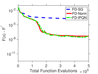
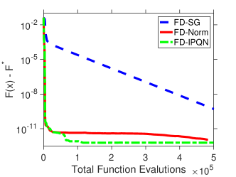
Figure 1: Chebyquad function results for a single run: Using $f_{\rm abs}$ (left column) and $f_{\rm rel}$ (right column) with $\sigma=10^{-3}$ (top row) and $\sigma=10^{-5}$ (bottom row).

Acknowledgments

This material was based upon work supported by the U.S. Department of Energy, Office of Science, Office of Advanced Scientific Computing Research, applied mathematics and SciDAC programs under Contract No. DE-AC02-06CH11357.

Supplementary Material

Finite-difference approximation error.

For any $\nu>0$ and any function $f(\cdot,\zeta)$ with $L$-Lipschitz continuous gradients, we have that

$$\|\nabla F^{\textrm{FD}}_{S_{k}}(x_{k})-\nabla F_{S_{k}}(x_{k})\|^{2} =\sum_{j=1}^{d}\left(\frac{1}{|S_{k}|}\sum_{\zeta_{i}\in S_{k}}\left(\frac{f(x_{k}+\nu e_{j},\zeta_{i})-f(x_{k},\zeta_{i})}{\nu}-\left[\nabla_{x}f(x_{k},\zeta_{i})\right]_{j}\right)\right)^{2}$$

$$\leq\sum_{j=1}^{d}\frac{1}{|S_{k}|}\sum_{\zeta_{i}\in S_{k}}\left(\frac{f(x_{k}+\nu e_{j},\zeta_{i})-f(x_{k},\zeta_{i})}{\nu}-\left[\nabla_{x}f(x_{k},\zeta_{i})\right]_{j}\right)^{2}$$

$$\leq\sum_{j=1}^{d}\frac{1}{|S_{k}|}\sum_{\zeta_{i}\in S_{k}}\left(\frac{L\nu}{2}\right)^{2}=\left(\frac{L\nu}{2}\right)^{2}d,$$

where the first equality is by the definitions of $\nabla F_{S_{k}}^{\textrm{FD}}(x_{k})$ and $\nabla F_{S_{k}}(x_{k})=\frac{1}{|S_{k}|}\sum_{\zeta_{i}\in S_{k}}\nabla_{x}f(x,\zeta_{i})$. The first inequality is due to the fact that $(a_{1}+a_{2}+\cdots+a_{n})^{2}\leq n(a_{1}^{2}+a_{2}^{2}+\cdots+a_{n}^{2})$, and the second inequality is due to

$$f(y,\zeta)\leq f(x,\zeta)+(y-x)^{T}\nabla_{x}f(x,\zeta)+\frac{L}{2}\|y-x\|^{2},\quad\forall x,y\in{\mathbb{R}}^{d}.$$

In a similar manner, we can show that, for the true gradients, the error due to finite-difference approximation is bounded. That is,

$$\|\nabla F^{\textrm{FD}}(x_{k})-\nabla F(x_{k})\|^{2} =\sum_{j=1}^{d}\left(\frac{F(x+\nu e_{j})-F(x)}{\nu}-\left[\nabla F(x_{k})\right]_{j}\right)^{2}$$

$$\leq\left(\frac{L\nu}{2}\right)^{2}d.$$ (19)

Inner product quasi-Newton expected condition.

Consider the following:

$$\mathbb{E}_{S_{k}}[(H_{k}\nabla F_{S_{k}}^{\textrm{FD}}(x_{k}))^{T}(H_{k}\nabla F(x_{k}))] =(H_{k}\nabla F^{\textrm{FD}}(x_{k}))^{T}(H_{k}\nabla F(x_{k}))$$

$$=(H_{k}(\nabla F^{\textrm{FD}}(x_{k})-\nabla F(x_{k})))^{T}(H_{k}\nabla F(x_{k}))+\|H_{k}\nabla F(x_{k})\|^{2},$$

where we used

$$\mathbb{E}_{S_{k}}[\nabla F^{\textrm{FD}}_{S_{k}}(x_{k})]=\mathbb{E}_{S_{k}}\left[\frac{1}{|S_{k}|}\sum_{\zeta_{i}\in S_{k}}\left[\frac{f(x_{k}+\nu e_{j},\zeta_{i})-f(x_{k},\zeta_{i})}{\nu}\right]_{j=1}^{d}\right]=\nabla F^{\textrm{FD}}(x_{k}),$$

and we have,

$$(H_{k}(\nabla F^{\textrm{FD}}(x_{k}) -\nabla F(x_{k})))^{T}(H_{k}\nabla F(x_{k}))$$

$$\leq\|H_{k}\nabla F(x_{k})\|\|H_{k}\|\|\nabla F^{\textrm{FD}}(x_{k})-\nabla F(x_{k})\|$$

$$\leq\|H_{k}\nabla F(x_{k})\|\|H_{k}\|\frac{L\nu\sqrt{d}}{2},$$

where the last inequality is due to (19). Therefore,

$$\mathbb{E}_{S_{k}}[(H_{k}\nabla F_{S_{k}}^{\textrm{FD}}(x_{k}))^{T}(H_{k}\nabla F(x_{k}))] \geq\|H_{k}\nabla F(x_{k})\|^{2}-\|H_{k}\nabla F(x_{k})\|\|H_{k}\|\frac{L\nu\sqrt{d}}{2}$$

$$\geq\|H_{k}\nabla F(x_{k})\|\left(\|H_{k}\nabla F(x_{k})\|-\|H_{k}\|\frac{L\nu\sqrt{d}}{2}\right).$$

For any $x_{k}$ such that $\|\nabla F(x_{k})\|>\frac{\lambda_{\max}(H_{k})L\nu\sqrt{d}}{2\lambda_{\min}(H_{k})}$, where $\lambda_{\max}(H_{k}),\lambda_{\min}(H_{k})>0$ are the largest and smallest eigenvalues of $H_{k}$, respectively, it thus follows that

$$\mathbb{E}_{S_{k}}\left[(H_{k}\nabla F_{S_{k}}^{\textrm{FD}}(x_{k}))^{T}(H_{k}\nabla F(x_{k}))\right]>0.$$

Numerical experiments setup.

In the tests of the proposed algorithm, we use $\theta=0.9$, finite-difference parameter $\nu=10^{-8}$, L-BFGS memory parameter $m=10$, and line search parameters ($c_{1}=10^{-4}$, $\tau=0.5$). None of these parameters have been tuned to the problems being considered.

The submitted manuscript has been created by UChicago Argonne, LLC, Operator of Argonne National Laboratory (“Argonne”). Argonne, a U.S. Department of Energy Office of Science laboratory, is operated under Contract No. DE-AC02-06CH11357. The U.S. Government retains for itself, and others acting on its behalf, a paid-up nonexclusive, irrevocable worldwide license in said article to reproduce, prepare derivative works, distribute copies to the public, and perform publicly and display publicly, by or on behalf of the Government. The Department of Energy will provide public access to these results of federally sponsored research in accordance with the DOE Public Access Plan. http://energy.gov/downloads/doe-public-access-plan.

References

• Audet and Hare [2017] C. Audet and W. L. Hare. Derivative-Free and Blackbox Optimization. Springer, 2017. doi: 10.1007/978-3-319-68913-5.
• Berahas et al. [2016] A. S. Berahas, J. Nocedal, and M. Takác. A multi-batch L-BFGS method for machine learning. In Advances in Neural Information Processing Systems, pages 1055–1063, 2016.
• Bertsekas [2019] D. P. Bertsekas. Reinforcement Learning and Optimal Control. Athena Scientific, 2019.
• Blanchet et al. [2019] J. Blanchet, C. Cartis, M. Menickelly, and K. Scheinberg. Convergence rate analysis of a stochastic trust region method via submartingales. INFORMS Journal on Optimization, 2019. URL https://arxiv.org/abs/1609.07428. To appear.
• Bollapragada et al. [2018a] R. Bollapragada, R. Byrd, and J. Nocedal. Adaptive sampling strategies for stochastic optimization. SIAM Journal on Optimization, 28(4):3312–3343, 2018a.
• Bollapragada et al. [2018b] R. Bollapragada, J. Nocedal, D. Mudigere, H. Shi, and P. Tang. A progressive batching l-BFGS method for machine learning. In Proceedings of the 35th International Conference on Machine Learning, volume 80 of Proceedings of Machine Learning Research, pages 620–629, 2018b.
• Byrd et al. [2012] R. H. Byrd, G. M. Chin, J. Nocedal, and Y. Wu. Sample size selection in optimization methods for machine learning. Mathematical Programming, 134(1):127–155, 2012.
• Fletcher [1965] R. Fletcher. Function minimization without evaluating derivatives – a review. The Computer Journal, 8:33–41, 1965. doi: 10.1093/comjnl/8.1.33.
• Fu et al. [2005] M. C. Fu, F. W. Glover, and J. April. Simulation optimization: A review, new developments, and applications. In Proceedings of the Winter Simulation Conference. IEEE, 2005. doi: 10.1109/wsc.2005.1574242.
• Hashemi et al. [2014] F. S. Hashemi, S. Ghosh, and R. Pasupathy. On adaptive sampling rules for stochastic recursions. In Proceedings of the Winter Simulation Conference 2014, pages 3959–3970. IEEE, 2014.
• Kim et al. [2015] S. Kim, R. Pasupathy, and S. G. Henderson. A guide to sample average approximation. In M. Fu, editor, Handbook of Simulation Optimization, volume 216 of International Series in Operations Research & Management Science, pages 207–243. Springer, 2015. doi: 10.1007/978-1-4939-1384-8_8.
• Larson et al. [2019] J. Larson, M. Menickelly, and S. M. Wild. Derivative-free optimization methods. Acta Numerica, 28:287–404, 2019. doi: 10.1017/s0962492919000060.
• Mania et al. [2018] H. Mania, A. Guy, and B. Recht. Simple random search of static linear policies is competitive for reinforcement learning. In Advances in Neural Information Processing Systems 31, pages 1800–1809. Curran Associates, Inc., 2018.
• Moré and Wild [2012] J. J. Moré and S. M. Wild. Estimating derivatives of noisy simulations. ACM Transactions on Mathematical Software, 38(3):19:1–19:21, 2012. doi: 10.1145/2168773.2168777.
• Pasupathy and Ghosh [2013] R. Pasupathy and S. Ghosh. Simulation optimization: A concise overview and implementation guide. In Theory Driven by Influential Applications, pages 122–150. INFORMS, 2013. doi: 10.1287/educ.2013.0118.
• Pasupathy et al. [2018] R. Pasupathy, P. Glynn, S. Ghosh, and F. S. Hashemi. On sampling rates in simulation-based recursions. SIAM Journal on Optimization, 28(1):45–73, 2018.
• Salimans et al. [2017] T. Salimans, J. Ho, X. Chen, S. Sidor, and I. Sutskever. Evolution strategies as a scalable alternative to reinforcement learning. Technical Report 1703.03864, ArXiv, 2017. URL https://arxiv.org/abs/1703.03864.
• Schraudolph et al. [2007] N. N. Schraudolph, J. Yu, and S. Günter. A stochastic quasi-Newton method for online convex optimization. In International Conference on Artificial Intelligence and Statistics, pages 436–443, 2007.