High Energy Photon Collider

Abstract

We discuss a high-energy photon linear collider (HE PLC) based on the $e^{+}e^{-}\,$  linear collider with cms electron energy $2E=1\div 2$ TeV (JLC, CLIC,…). This energy region was previously considered hopeless for experiment. On the contrary, the present study leads to a rather optimistic conclusions. We compare properties of HE PLC with those of the usually discussed standard PLC with $E\approx 250$ GeV. We show that at the optimal choice of laser the high-energy $\gamma\gamma\,$luminosity integral is about 1/5, and the maximum luminosity is about 1/4 from similar values for the standard PLC. For this choice, the laser flash energy and laser-optical system should be approximately the same as those prepared for the standard PLC. The photon spectrum of HE PLC is much more monochromatic than that in the standard PLC, it is concentrated near the high-energy limit with an energy spread of about 5%. It will be well separated from the low energy part.

1 Introduction

Two photon processes – virtual vs real photons.

A process belonging to the class of what is now called two-photon was first considered in 1934. This was the production of $e^{+}e^{-}\,$ pairs in the collision of ultrarelativistic charged particles, $A_{1}A_{2}\to A_{1}A_{2}+X$ with $X=\mbox{$e^{+}e^{-}\,$}$ [1]. Next 35 years different authors considered similar processes with $X=\mu^{+}\mu^{-}$, $X=\pi^{+}\pi^{-}$ (point-like), $X=\pi^{0}$ (see references in review [2]). In 1970, it was shown that observing the processes $A_{1}A_{2}\ toA_{1}A_{2}+X$ at colliders (primarily at $e^{+}e^{-}\,$colliders) will allow us to study the processes $\mbox{$\gamma\gamma\,$}\to X$ with two quasi-real photons at very high energies [3] (and a little later [4]).

The general description of such processes given in the review [2] is relevant till now. The collision of particles $A_{i}$ with mass $M_{i}$, electric charge $Z_{i}e$ and energy $E_{i}$ produces two virtual (quasi-real) photons with energies $\omega_{i}$. Their fluxes (per initial particle $A_{i}$) are

$$f(\omega_{i})d\omega_{i}\approx\dfrac{{Z_{i}\alpha}}{{\pi}}\,g_{i}(\omega_{i}/E_{i})\,\dfrac{{d\omega_{i}}}{{\omega_{i}}}\,L_{i}\;\theta(L_{i})\,,\quad L_{i}\approx\ln\left(\lambda_{q}^{2}(E_{i}/M_{i})^{2}/\omega_{i}^{2}\right)\,,$$

where the form of the function $g_{i}(x)\leqslant 1$ and the parameter $\lambda_{q}$ depend on the type of collided particle $A_{i}$ and on the properties of the system $X$. Thus, the experiments with quasi-real photons became a natural part of the collider experiments (see, for example, [5]). They made important additions to our knowledge of the resonances and details of hadron physics. However, they are not competitive with the studies of New Physics on $e^{+}e^{-}\,$and $pp$ colliders. Indeed, in the high-energy part the luminosity of virtual photon collisions is 3-5 orders of magnitude lower than that of the base $e^{+}e^{-}\,$or $pp$ collider. For a collision of heavy nuclei (RHIC, LHC), the effective energy spectrum of virtual photons is limited from above and difficulties with the signature of $\gamma\gamma\,$events are added. Therefore, studying the effects of New Physics is very difficult or impossible in collision of virtual photons at all these colliders.

Quite different approach allowing to obtain $\gamma\gamma\,$collisions with the real photons and to use them for study the phenomena of New Physics was developed in 1981 [6] when discussing the potential of $e^{+}e^{-}\,$linear colliders (with electron energies $E$). In these colliders, each electron bunch is used only once. Therefore, one can try to convert a significant fraction of incident electrons into photons with energy $\omega\sim E$ so that the resulting $\gamma\gamma\,$collisions compete with the main $e^{+}e^{-}\,$collision in both the collision energy and luminosity.

Photon Colliders with real photons – PLC.

This option – Photon Linear Collider (PLC) was proposed by our group [6] as a specific mode of future $e^{+}e^{-}\,$ linear collider (LC) [7]-[11]. PLC will be useful both for clarifying the results obtained at the hadron collider (LHC type) or $e^{+}e^{-}\,$colliders – linear (ILC, CLIC,…) or circular (FCC-ee, CEPC,…) – and for solving New Physics problems that are inaccessible or very difficult to study at these colliders

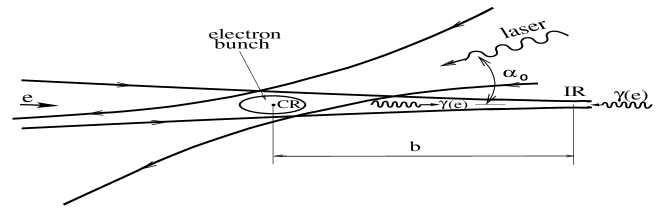
Figure 1: Scheme of PLC

The well-known scheme of   PLC is shown in fig. 1. At conversion region $CR$ preceding the interaction region $IR$, electron ($e^{-}$ or $e^{+}$) beam of the basic LC meets the photon flash from the powerful laser. The Compton backscattering of laser photons on electrons from LC produces high energy photons. With the suitable choice of laser one can obtain photon beams with the photon energies close to that of the initial electron. These photons are focused in the interaction region at the approximately the same spot, as it was expected for electrons without laser conversion. As a result, the $\gamma\gamma\,$ or $e\gamma\,$ collisions under interest occur in the interaction region. The ratio of number of high energy photons to that of electrons – the conversion coefficient $k\sim 1$, for the standard PLC $k\approx 1-1/e\approx 0.63$ typically. Numerous studies of PLC (see, for example, [7], [8]) are developing many new technical details, but all of them keep the initial scheme fig. 1.

Main properties of the basic Compton process are determined by the parameter

$$x=4E\omega_{0}/m_{e}^{2}\,,$$ (1)

where $E$ is the electron beam energy and $\omega_{0}$ – the laser photon energy. (To simplify text, we set $\alpha_{0}$ in Fig. 1 to be zero.)

The most suitable modern lasers with neodymium glass or garnet allow to realize such scheme in its pure form only for the electron beam energy $E\leqslant 270$ GeV (first stage of ILC). For $x>2(1+\sqrt{2})\approx 4.8$ (at $E>270$ GeV using the same laser) some of produced high energy photons die out, producing $e^{+}e^{-}\,$pairs in the collisions with laser photons from the tail of laser flash. This fact was treated as limiting for realization of PLC based on LC with higher electron energy [6]). To overcome this difficulty, two alternatives were discussed:

$\triangledown$ to use a new laser with lower photon energy;

$\triangledown$ to use existing lasers and accept a reduction in $\gamma\gamma\,$ luminosity.

$\triangledown$ For the first alternative, the results of [6] are applicable. Only for each new energy of electrons a new laser is needed, and such lasers with the necessary parameters do not exist.

$\triangledown$ We consider the second alternative, following the idea that it is important to generate clean photon collisions even at the expense of some reduction in luminosity.
This opportunity was mention in papers [12, 13] but the detailed analysis of processes appeared at $x>4.8$, optimization of condition for $e\to\gamma$ conversion and influence of these new processes for properties of obtained $\gamma\gamma\,$collider were absent in literature. And these problems are the main subject of the present paper.

We will show that in this approach at electron beam energy up to 1 TeV one can obtain reasonable high energy luminosity with the very narrow energy distribution. The laser system developed for PLC at the first stage of LC (for standard PLC) can be applied here with the minimal variations (obliged mainly by change of the initial electron beam). To reach luminosity close to the best possible one, the necessary laser flash energy should be enhanced by about 50% only.

The organization of text is following. Sections 2 and 3 are introductory. In the sect. 2 we summarize main assumptions, technical points and notations. Sect. 3 is devoted to the description of customary facts related to PLC at $x<4.8$ with examples for the case $x=4.5$.

After that in the main body of the paper we consider cases with $x=9$ and 18 which correspond to the initial electron beam energy 500 GeV and 1000 GeV (ILC, CLIC), and present some examples for $x=100$ (the electron beam energy 5 TeV) – sect. 4. We consider the high energy part of spectra, which is well separated from their low energy part. We start this description from the discussion of process $\gamma\gamma_{o}\to\mbox{$e^{+}e^{-}\,$}$ (“killing process”) in the conversion region (see notations below). This process is absent at lower energies considered in earlier papers, i.e. at $x<4.8$. After a brief discussion of the basic Compton effect at $x>4.8$ (sect. 4.2), we present equations for balance of photons, produced in the Compton process and disappeared in the the conversion region due to killing processes – sect. 4.3.

Next point is the optimal choice of the laser flash energy which correspond to the choice of the optical length for the laser flash. This choice is provided the maximal number of photons for physical studies under interest (sect. 5). The sect. 6 contains main results of the paper – the description of high energy luminosity spectra for $e\gamma\,$ and $\gamma\gamma\,$ collisions.

Summary (sect. 7) presents a brief description of the obtained results. In this respect it is interesting to note the following fact. It is natural to expect that the shape of the resulting photon spectrum will differ markedly from that of the basic Compton effect. To our surprise, the difference was not very large if we use a reasonable choice of the polarization for the initial beams. It is due to fact that the effects of the energy dependence are compensated by changing the polarization.

In Appendix A.1 we discuss case of “bad” choice of initial polarization. In Appendix A.2, we show that the HE PLC studies with linear polarization of high energy photons are practically impossible. Most important background is discussed in Appendix A.3. In Appendix B we briefly discusses New Physics problems that cannot be studied using LHC and $e^{+}e^{-}\,$colliders and which can be studied using HE PLC.

2 Introduction. Technical

The principal assumptions and notations.

For definiteness, we consider as a basic the $e^{-}e^{-}$ LC (not $e^{+}e^{-}$). We consider the effects of high photon density in the conversion region (nonlinear QED effects) to be negligible.
Notations.

• $\gamma_{o}$, $\omega_{o}$, $\lambda_{o}$ – the laser photon, its energy and helicity;

• $e_{o}$, $E$, $\lambda_{e}$ – the initial electron, its energy and helicity ($2|\lambda_{e}|\leqslant 1$);

• $\gamma$, $\omega$, $\lambda$ – the produced photon, its energy and helicity;

• $\sigma_{0}=\pi r_{e}^{2}=\;2.5\cdot 10^{-25}\;\mbox{cm}^{2}$;

• $b$ – the distance between the conversion region $CR$ and the interaction region $IR$ (Fig. 1);

• $\Lambda_{C}=2\lambda_{e}\lambda_{o}$ – ”polarization of the process”;

• $y=\omega/E$ – relative photon energy;

• $y_{M}=x/(x+1)$ – maximal value of $y$ at given $x$;

• $w_{\gamma\gamma}=\dfrac{{\sqrt{4\omega_{1}\omega_{2}}}}{{2E}}\equiv\sqrt{y_{1}y_{2}}\leqslant y_{M}$ and $w_{e\gamma}=\dfrac{{\sqrt{4E\omega_{1}}}}{{2E}}\equiv\sqrt{y_{1}}\leqslant\sqrt{y_{M}}$ – ratios of the $\gamma\gamma\,$  and $e\gamma\,$ cms energies to $\sqrt{s}=2E$.

We consider relative luminosities $\cal L$, and high energy luminosity integral

$$\begin{gathered}L_{exp}(w)={\cal L}(w)\cdot L_{geom},\\ {\cal L}_{h.e.}=\!\!\int\limits_{y_{min}}^{1}\!\!{\cal L}(w)dw\;\;\left(w=w_{e\gamma}\;\;or\;\;w_{\gamma\gamma}\right).\end{gathered}$$ (2)

The quantity $y_{min}$ here is the position of a minimum in the energy distribution of Compton photons at $x>3$ and $\Lambda_{C}\approx-1$, it depends on $x$ – see (9) and Table 3. (The choice of this quantity does not require high accuracy, since the number of Compton photons at $y\approx y_{min}$ is small.)

Here $L_{geom}$ is luminosity of the $e^{-}e^{-}$ collider prepared for $\gamma\gamma\,$ mode. In a nominal ILC option, i.e. at the electron beam energy of 250 GeV, the geometric luminosity can reach $L_{geom}=12\cdot 10^{34}$ cm^-2s^-1 which is about 4 times greater then the anticipated $e^{+}e^{-}\,$luminosity.

All numerical calculations are carried out for the case of a ”good” polarization of collided electrons and photons $\Lambda_{C}\approx-1$, in two versions: $\Lambda_{C}=-1$ and $\Lambda_{C}=-0.86$ (more realistic case).

We distinguish luminosities $L_{I}$ with different total helicity$I=|\lambda_{1}-\lambda_{2}|$ of initial state, that are ($L_{1/2}$ and $L_{3/2}$ for $e\gamma\,$collisions) and ($L_{0}$ and $L_{2}$ for $\gamma\gamma\,$ collisions). We find that one of these helicities dominates in the most important and useful high energy part of the luminosity spectrum. Therefore, below we discuss total luminosity (sum over both final helicities) and present fraction of final state, giving smallest contribution into luminosity. Trivial change of sign of helicity of one electron and laser beam allows produce states with total helicity 2 instead 0 – for $\gamma\gamma\,$ collisions and 3/2 instead of 1/2 – for $e\gamma\,$collisions.

$\bullet$ The obtained luminosity spectra can be treated as the sum of two separate distributions.

$\triangledown$ We are only interested in the high-energy part of the luminosity spectrum. It is formed by photons obtained in the basic Compton process (5a), some of these photons die in the processes (5c). An important feature of the Compton effect for $x>3$ is as follows: with a suitable polarization of the colliding electrons and laser light, the high-energy part of the resulting photon spectrum is well separated from the low-energy part, and this separation is enhanced with increasing electron energy $E$. The dependence of details of experimental device can be eliminated from description of this part [14] – see discussion around Eq. (12).

$\triangledown$ The low-energy part of photon spectra is formed by low energy photons from the basic Compton process (5a) and photons from the scattering of laser photons from the tail of the laser bunch (i) on electron after the first Compton process (5b) or (ii) on positrons or electrons produced in the killing process (LABEL:parasitic). The shape of the energy distribution in this region depends on details of the experimental device.

$\bullet$ Below, the laser bunch is assumed to be wide enough so that a change in its density inside the electron bunch can be neglected.

The optical length of the laser bunch for electrons is expressed via the longitudinal density of photons $n_{L}$ in flash (that is via the laser bunch energy $A$ divided to its effective transverse cross section $S_{L}$) and the total cross section of the Compton scattering $\sigma_{C}(x,\Lambda_{C})$:

$$z=\dfrac{{A}}{{\omega_{o}S_{L}}}\,\sigma_{C}(x,\Lambda_{C})\equiv\dfrac{{A}}{{A_{0}}}\dfrac{{\sigma_{C}(x,\Lambda_{C})}}{{\sigma_{C}(x\!=\!4.5,\Lambda_{C}\!=\!-1)}}\,.$$ (3)

In the last form of this equation we introduce $A_{0}$ – the laser flash energy, necessary to obtain $z=1$ at $x=4.5$, $\Lambda_{C}=-1$.

When the electrons traverse the laser beam, their number decreases as

$$n_{e}(z)=n_{eo}e^{-z}\,.$$ (4)

$x$	4.5	9	18	100
$\Lambda_{C}\!=\!-1$	0.73	0.45	0.26	0.056
$\Lambda_{C}=1$	0.85	0.63	0.44	0.145

Table 1: Compton cross section $\sigma_{C}/\sigma_{0}$ at different $x$ and polarizations

$\bullet$ For the most suitable modern laser with $\omega_{o}=1.17$ eV at$E=250$ GeV we have $x=4.5$. For the next stages of LC projects with $E=500$ GeV and $1000$ GeV we have $x=9$ and $x=18$ respectively. The process (5c), killing high energy photons, is switched on at ${x>2(1+\sqrt{2})\approx 4.8}$.

Processes in the conversion region.

Let us list processes in the conversion region:

$$e_{o}\gamma_{o}\to e\gamma\; \mbox{\it basic Compton process};$$ (5a)

$$e\gamma_{o}\to e\gamma\;;$$ rescattering (5b)

$$\gamma\gamma_{o}\to\mbox{$e^{+}e^{-}\,$}; \mbox{\it killing process};$$ (5c)

$$e^{\pm}\gamma_{o}\to e^{\pm}\gamma\;;$$ (5d)

$$e_{o}\gamma_{o}\to e\mbox{$e^{+}e^{-}\,$}\; \mbox{\it Bethe-Heitler process}\,.$$ (5e)

$\bullet$   The Bethe-Heitler process (5e), switching on at $x=8$, is the process of the next order in $\alpha$ but its cross section does not decrease with growth of energy, in contrast to the Compton process:

$\sigma_{BH}=(28/9\pi)\alpha\sigma_{0}(\ln x-109/42)\;\;$ at $x\gg 1$.

$x$	30	100	300
$\Lambda_{C}=-1$	0.96	0.80	0.47
$\Lambda_{C}=1$	0.97	0.88	0.62

Table 2: Factor $K_{BH}$

Because of this process, the yield of high-energy photons decreases by the factor

$$K_{BH}=\dfrac{{\sigma_{C}(x)}}{{\sigma_{C}(x)+\sigma_{BH}(x)}}\,,$$ (6)

and the $\gamma\gamma\,$ luminosity reduces by the factor $K_{BH}^{2}$. The numerical values of this factor are presented in the Table 2. It shows that the Bethe-Heitler mechanism is negligible at $x<100$, the reduction of the photon yield becomes unacceptably large at $x>300$.

3 Basics

Before main discussion, we repeat some basic points from papers [6] in the form, suitable for description of high energy part of spectra at large $x$, with addition of some details which were not discussed previously.

In this section numerical examples are given for the standard case $x=4.5$, which is close to the upper limit of validity in previous studies. The photon energy is kinematically bounded from above by quantity $y_{M}=x/(x+1)$. For $x=4.5$ we have $y\leqslant y_{M}=0.82$.

The total cross section of Compton effect is well known (Table 1):

$$\begin{gathered}\sigma_{C}=\dfrac{{2\sigma_{0}}}{{x}}\left[F(x)+\Lambda_{C}T(x)\right],\\ F(x)\!=\!\left(1-\dfrac{{4}}{{x}}\!-\!\dfrac{{8}}{{x^{2}}}\right)\ln(x+1)\!+\!\dfrac{{1}}{{2}}\!+\!\dfrac{{8}}{{x}}\!-\!\dfrac{{1}}{{2(x+1)^{2}}},\\ T(x)\!=\!\left(1\!+\!\dfrac{{2}}{{x}}\right)\ln(x+1)\!-\!\dfrac{{5}}{{2}}\!+\!\dfrac{{1}}{{x+1}}\!-\!\dfrac{{1}}{{2(x+1)^{2}}}.\end{gathered}$$ (7)

The photon energy distribution at $E\gg\omega_{o}$ is given by
($r=\dfrac{{y}}{{x(1-y)}}\leqslant 1$)

$$\begin{gathered}f(x,y)\!\equiv\!\dfrac{{1}}{{\sigma_{C}}}\,\dfrac{{d\sigma_{C}}}{{dy}}=\dfrac{{U(x,y)}}{{F(x)+\Lambda_{C}T(x)}}\equiv\\ \!\equiv\!\dfrac{{\left[\dfrac{{1}}{{1-y}}\!+\!1\!-\!y\!-\!4r(1\!-\!r)\!-\!\Lambda_{C}\,xr(2\!-\!y)\,(2r\!-\!1)\right]}}{{F(x)+\Lambda_{C}T(x)}}.\end{gathered}$$ (8)

Figure 2: Photon energy spectrum $f(x,y)$ at $x=4.5$, $\Lambda_{C}=-1$ (solid) and $\Lambda_{C}=1$ (dotted)

The shape of this distribution depends strongly on both $x$ and polarization of process. At $\Lambda_{C}\approx-1$, the photon spectrum grows up to its upper boundary $y=y_{M}$, at $\Lambda_{C}\approx 1$ this spectrum is much more flat (Fig. 2).

At $x>3$ and $\Lambda_{C}\approx-1$ the high energy part of this distribution is concentrated in the narrow strip below upper limit, contained more than one half produced photons. We characterize this peak by its lower boundary $y_{min}$ and sharpness parameter $\tau$ – see Table 3

$$\begin{gathered}\mbox{\it definition of $y_{min}$:}\;\;\quad\int\limits_{y_{min}}^{y_{M}}f(x,y)dy\approx 0.55;\\ f(x,y\leqslant y_{min})\ll f(x,y_{M})\,;\\ \mbox{\it definition of $\tau$:}\quad f(x,y=y_{M}(1-\tau))=\dfrac{{1}}{{2}}\cdot f(x,y_{M})\,.\end{gathered}$$ (9)

x	4.5	9	18	100
$y_{min}$	0.6	0.7	0.75	0.94
$\tau$		0.036	0.022

Table 3: Properties of high energy peak at $\Lambda_{C}\approx-1$

The mean circular polarization (helicity) of the produced photon is

$$\begin{gathered}\lambda_{C}(y)=\\ =\dfrac{{-\lambda_{o}(2r\!-\!1)[(1-y)^{-1}\!+\!1-\!y]\!+\!2\lambda_{e}xr[1\!+\!(1\!-\!y)(2r\!-\!1)^{2}]}}{{U(x,y)}}.\end{gathered}$$ (10a)

At $$\lambda_{o}=\pm 1$$, this equation is simplified:

$$\!\!\lambda_{C}(y)\!=\!-\!\lambda_{o}\left[(2r\!-\!\!1)\!+\!\dfrac{{\left[(2r-1)-\Lambda_{C}xr\right]4r(1-r)}}{{U(x,y)}}\right]\!.$$ (10b)

The photons of highest energies are well polarized with the same direction of spin as laser photons, i. e. $\lambda_{C}(y=y_{M})=-\lambda_{o}$.

The photons of maximal energy move in the direction of the initial electron. With decreasing of the photon energy its escape angle grows as

$$\theta(y)=\dfrac{{m}}{{E}}\;\sqrt{x+1}\;\sqrt{\dfrac{{y_{M}}}{{y}}-1}.$$ (11)

The $\gamma\gamma\,$ or  $e\gamma\,$ luminosities are given by convolution of high energy photon spectrum with spectrum of collided photon or electron taking into account the mentioned spread of photons at the way from the conversion region $CR$ to the interaction region $IR$. Owing to the angular spread (11), at this way more soft photons spread for more wide area, and collide more rare, as a result, their contribution to luminosity decreases. Therefore, with the growth of the distance $b$ between the conversion region $CR$ and the interaction region $IR$ luminosity decreases but monochromaticity improves. At $y>y_{M}/\sqrt{2}$  these effects are described with good accuracy by a single parameter – as for round beam [14]

$$\rho^{2}=\left(\dfrac{{b}}{{(E/m_{e})\sigma_{x}}}\right)^{2}+\left(\dfrac{{b}}{{(E/m_{e})\sigma_{y}}}\right)^{2}\,.$$ (12)

(Here $\sigma_{x}$ and $\sigma_{y}$ are semiaxes of ellipse, described initial electron beam in the would be interaction point. In this approximation, the discussed luminosities are expressed via distributions in the photon energy [6]:

$$\dfrac{{dL_{\gamma e}^{\lambda}}}{{dy}}=n_{e}n_{\lambda}(y,z)e^{-\dfrac{{\rho^{2}\phi^{2}}}{{2}}}\,\quad\left(\phi_{a}=\sqrt{y_{M}/y_{a}-1}\right);$$ (13)

$$\!\!\!\!\dfrac{{dL_{\gamma\gamma}^{2,\lambda_{1}\lambda_{2}}}}{{dy_{1}dy_{2}}}\!=\!n_{\lambda_{1}}(y_{1},z)n_{\lambda_{2}}(y_{2},z)I_{0}(\rho^{2}\phi_{1}\phi_{2})e^{-\,\dfrac{{\rho^{2}(\phi_{1}^{2}+\phi_{2}^{2})}}{{2}}}\,.$$ (14)

Here $I_{0}(z)$ is the modified Bessel function. The distributions over the center of mass energy $w$ are obtained by the substitution$w=\sqrt{y}$  for $e\gamma\,$ luminosity or $w=\sqrt{y_{1}y_{2}}$ with simple integration, for $\gamma\gamma\,$ luminosity.

At $x\leqslant 4.8$ each missed electron produces the photon. Therefore at $z=1$ and $\rho=0$   total $e\gamma\,$ and $\gamma\gamma\,$ luminosities are

$${\cal L}_{e\gamma}=(1-1/e)=0.63\,,\qquad{\cal L}_{\gamma\gamma}=(1-1/e)^{2}=0.4.$$ (15)

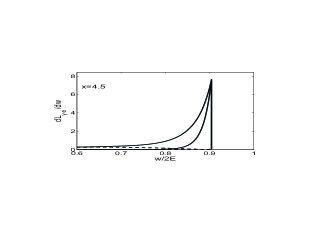
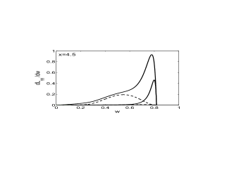
Figure 3: Luminosity spectra $dL/dw$ at $x=4.5$, $\Lambda_{C}=-1$, $z=1$ for $\rho=1$ (up) and $\rho=5$ (down) – solid lines, dotted lines – similar distributions at $\rho=1$ for final states with total helicity $3/2$ for $e\gamma\,$ collisions (left) and total helicity 2 for $\gamma\gamma\,$ collisions ( right).

Fig. 3 and first lines of Tables 5, 6 represent $\gamma\gamma\,$  and  $e\gamma\,$ luminosity distributions in their cms energy at $\Lambda_{C}=-1$, $z=1$ for $\rho=1$ and 5.

At $\Lambda_{C}=-1$ and $\rho\geqslant 1$, the main part of calculated luminosity is concentrated at $w>0.6$ (in particular, the $e\gamma\,$ luminosity spectrum at $y>0.6$ contains about 2/3 of produced photons). The relative values of luminosity with total helicity 2 for $\gamma\gamma\,$ collisions and luminosity with total helicity 3/2 for $e\gamma\,$ collisions are small and decrease quickly with growth of $\rho$, it means that the colliding photons become practically monochromatic in their polarization.

Therefore, we describe the luminosity distribution by three parameters:
1) the integral ${\cal{L}}_{h.e.}$ (2),
2) the relative value of contribution with total helicity 2 or $3/2$,
3) position of maximum $w_{M}$ in summary luminosity and corresponding maximal value $L(w_{M})$. (For $e\gamma\,$ collisions peak is disposed at the maximal value of $w=\sqrt{y_{M}}$, and $L(w_{M})$ is independent on $\rho$).

4 At $\boldsymbol{x\geqslant 4.8}$

In principle, all processes (5) should be taken into account. Only two of them, basic Compton effect (5a) (discussed in previous section) and killing process (5c) take part in formation of high energy part of photon spectrum under interest. The process (LABEL:parasitic) adds low energy photons like the process (5b). The contribution of these processes into high energy part of photon spectrum is small at considered moderate conversion coefficients.

4.1 Killing process (5c)

The killing process describes the disappearance of a Compton high-energy photon in its collision with a laser photon from the tail of a bunch, generating $e^{+}e^{-}\,$ pair, it switches on at $x\approx 4.8$. For the photon with energy $yE$ the squared cms energy for process is $w^{2}_{k}=4\omega\omega_{o}/m_{e}^{2}=xy>4$. Its cross section is

$$\begin{gathered}\sigma_{kill}(w^{2}_{k},\lambda_{o}\lambda)=\dfrac{{4\sigma_{0}}}{{w^{2}}}\Phi_{\mbox{$\gamma\gamma\,$}}(w^{2}_{k},\lambda_{o}\lambda)\,,\\ \Phi_{\mbox{$\gamma\gamma\,$}}(w^{2}_{k},\lambda_{o}\lambda)=\left(1+\dfrac{{4}}{{w^{2}_{k}}}-\dfrac{{8}}{{w^{4}_{k}}}\right)L-\\ -\left(1+\dfrac{{4}}{{w^{2}_{k}}}\right)v-\lambda_{o}\lambda(L\!-\!3v),\\ v=\sqrt{1-4/w^{2}_{k}\;},\quad L=2\ln\left(\dfrac{{w_{k}}}{{2}}(1+v)\right);\\ w^{2}_{k}=\dfrac{{4\omega_{o}\omega}}{{m_{e}^{2}}}\equiv xy\,.\end{gathered}$$ (16)

Note that

$$\begin{gathered}\dfrac{{\sigma_{kill}(\lambda_{o}\lambda>0)}}{{\sigma_{kill}(\lambda_{o}\lambda<0)}}>1\;\;\mbox{at}\;\;w^{2}_{k}<15;\\ \dfrac{{\sigma_{kill}(\lambda_{o}\lambda>0)}}{{\sigma_{kill}(\lambda_{o}\lambda<0)}}<1\;\;\mbox{at}\;\;w^{2}_{k}>15.\end{gathered}$$ (17)

4.2 Basic spectra

The photon energy spectra for the basic Compton backscattering (8) at $x=9$ is shown in Fig. 4 – left.

It is clearly seen that this spectrum for $\Lambda_{C}=-1$ is concentrated near the high energy limit strongly then the corresponding spectrum for $x=4.5$ in Fig. 2.

At $x=18$ similar calculations show that the spectrum is concentrated in the narrow strip $0.85<y\equiv\omega/E<0.95$. At $\Lambda_{C}=1$ these spectra are much more uniform, without the big peak at high energies.

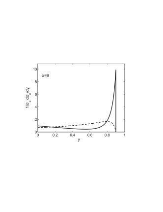
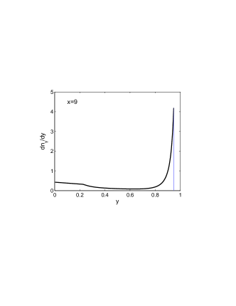
Figure 4: The case $x=9$. Left – Compton spectrum of photons. Solid line corresponds to $\Lambda_{C}=-1$, dashed line – to $\Lambda_{C}=1$. Right – photon energy spectrum reduced by killing process at $\Lambda_{C}=-1$, $z=0.7$

4.3 Equations

The balance of high energy photons is given by their production in the Compton process (5a) and their disappearance at the production of $e^{+}e^{-}\,$ pairs in the collision of these photons with residual laser photon (killing process (5c)).

Let us denote by $n_{\gamma}(y,z,\lambda)$ the flux of photons (per 1 electron) with the energy $yE$ and polarization $\lambda$ after travelling inside the laser beam with the optical length $z$. It is useful for calculations to decompose this photon flux to the sum of fluxes of right polarized photons $n_{(\gamma+)}(y,z)$ and left polarized photons $n_{(\gamma-)}(y,z)$ so that the total photon flux $n_{\gamma}(y,z)$ and its average polarization $\lambda$ are

$$\begin{gathered}n_{\gamma}(y,z)=n_{(\gamma+)}(y,z)+n_{(\gamma-)}(y,z),\\ \langle\lambda(y,z)\rangle=\dfrac{{n_{(\gamma+)}(y,z)-n_{(\gamma-)}(y,z)}}{{n_{(\gamma+)}(y,z)+n_{(\gamma-)}(y,z)}}\,.\end{gathered}$$ (18)

Naturally, $\langle\lambda(y,z\to 0)\rangle\to\Lambda_{C}(y)$ from (10).

The variation of these fluxes during the travelling inside the laser bunch is described by equations

$$\begin{gathered}\dfrac{{dn_{(\gamma\pm)}(y,z)}}{{dz}}=\\ \!=\!\dfrac{{1}}{{2}}\left(1\pm\Lambda_{C}(y)\right)f(x,y)n_{e}(z)\!-\!n_{(\gamma\pm)}\dfrac{{\sigma_{kill}(xy,\pm\lambda_{o})}}{{\sigma_{C}(x)}}.\end{gathered}$$ (19)

The number of photons and their mean polarization are expressed via subsidiary quantities $\nu_{\pm}$:

$$\begin{array}[]{c}n_{\gamma}(y,z)=f(x,y)\nu(z,y),\\ \nu(z,y)=\nu_{+}(z,y)+\nu_{-}(z,y),\quad\langle\lambda\rangle=\dfrac{{\nu_{+}(z,y)\!-\!\nu_{-}(z,y)}}{{\nu(z,y)}}.\end{array}$$

The equation (19) is easily solved:

$$\begin{gathered}n_{(\gamma\pm)}(y,z)=f(x,y)n_{e0}\nu_{\pm}(y,z);\\ \mbox{where}\;\;\nu_{\pm}(y,z)=\dfrac{{\left(1\pm\Lambda_{C}(y)\right)}}{{2}}\cdot\dfrac{{e^{-\zeta_{\pm}z}-e^{-z}}}{{1-\zeta_{\pm}}};\\ \zeta_{\pm}=\dfrac{{\sigma_{kill}(xy,\pm\lambda_{o})}}{{\sigma_{C}(x)}}\,.\end{gathered}$$ (20)

It is useful for future discussions to define in addition ratio of number of killed photons to the number of photons, prepared for the $\gamma\gamma\,$ collisions, $r_{K}(y,z)$ – see Table 4.

In Fig.  4 we compare photon energy spectrum for the pure Compton effect (left plot) and after travelling inside the laser bunch with $z=0.7$ (right plot). One can see at the right plot that (1) the shape of the high-energy part of the spectrum reproduces approximately that for the pure Compton effect; (2) in the middle part of spectrum the killing process leads to relative decrease of spectrum; (3) the part of spectrum, correspondent to $xy<4$ is relatively enhanced, since at these $xy$ the killing process is absent.

5 Optimization

At $x<4.8$, the growth of the optical length results in monotonous increase of number of photons (with the simultaneous growth of background). On the contrary, at $x>4.8$, the killing process stops this increase and even kills all high energy photons at extremely large $z$. The dependence $n(y,z)$ on $z$ has maximum at some $z=z_{m}(y)$, which can be treated as the optimal value of $z$. However, what value of $y$ should we use?

The simplest approach is to consider this balance only for high energy photons, at $y=y_{M}$ [12]. We find it more reasonable to consider for this goal the $z$-dependence of entire luminosity within its high energy peak ${\cal L}_{h.e.}$ (2), (9), Table 3.

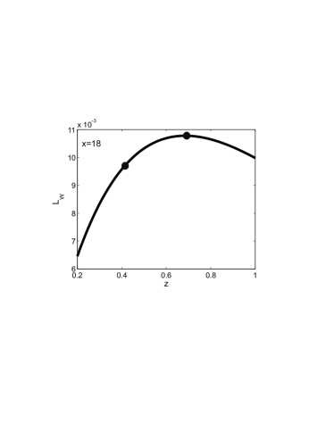
Figure 5: The $\gamma\gamma\,$ luminosity integral ${\cal L}_{h.e.}$ in dependence on $z$, for $\rho=1$, $\Lambda_{C}=-1$. Dots correspond $z_{m}$ and $z_{0.9}$.

The typical dependence of luminosity ${\cal L}_{h.e.}$ on $z$ is shown in Fig. 5. The curves at another $x$ and $\rho$ have similar form. The optimal value of the laser optical length are given by the position of a maximum at these curves, $z_{m}$ They are shown in the table 4. We find numerically that the dependence of $z_{m}$ on $\rho$ is negligibly weak.

The curves like Fig. 5 are very flat near maximum. Therefore, value $z_{0.9}(x)<z_{m}(x)$, provided luminosity which is 10% lower than maximal one, is noticeably less than $z_{m}$. In the table 4 we present for $\Lambda_{C}=-1$
(i) values $z_{m}$ and $z_{0.9}$;
(ii) laser flush energies (3) required to obtain either maximal luminosity $A(z_{m})$ or 90%  of this luminosity $A(z_{0.9})$ (in terms of the laser flush energy $A_{0}$, required to obtain $z=1$ at $x=4.5$);
(iii) the proportion of killed photons among all photons born in the basic Compton effect (at $y=y_{M}$) $r_{K}(z,y)$.

x	$y_{min}$	z	$r_{K}(z,y_{M})$	$A(z)/A_{0}$
9	0.7	$z_{m}=0.704$	0.22	1.15
		$z_{0.9}=0.49$	0.13	0.8
18	0.75	$z_{m}=0.609$	0.43	1.7
		$z_{0.9}=0.418$	0.28	1.17
100	0.94	$z_{m}=0.48$		6.3
		$z_{0.9}=0.32$		4.2

Table 4: Optical lengths $z_{m}$ and $z_{0.9}$, fraction of killed photons and necessary laser flash energy at these $z$ for $\Lambda_{C}=-1$

6 Luminosity distributions

Now we consider luminosity spectra for optimal $z=z_{m}$. The examples of these spectra for $\gamma\gamma\,$ and $e\gamma\,$ luminosities at $x=18$, $\Lambda_{C}=-1$ for $\rho=1$ and 5 are shown in Fig. 6. The curves for other $x$ and $\rho$ have similar form.

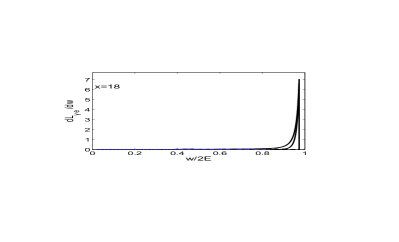
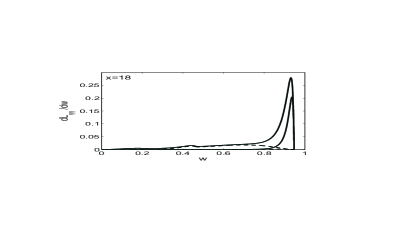
Figure 6: Luminosity spectra $dL/dw$ at $x=18$, $\Lambda_{C}=-1$, $z=1$ for $\rho=1$ (up) and $\rho=5$ (down) – solid lines; dotted lines – similar distributions for final states with total helicity $3/2$ ($\gamma e$  collisions) or 2 ($\gamma\gamma\,$ collisions).

$\bullet$ The table 5 represent main properties of high energy peaks in the $\gamma\gamma\,$  luminosity spectra at $x=9,\,18$ for $\Lambda_{C}=-1$ and $\Lambda_{C}=-0.86$ at optimal $z=z_{m}$. Lines for $x=4.5$, $z=1$ and $x=100$, $z=z_{m}$ are presented for comparison. Here
${\cal L}_{h.e.}$ — total luminosity of the high energy peak (2), Table 3,
$L_{m}=L(w_{M})$ – maximal differential luminosity,
$w_{M}$ – position of maximum in luminosity,
$w_{\pm}$ – solutions of equation $L(w_{\pm})=L(w_{M})/2$,
$\gamma_{w}=(w_{+}-w_{-})/w_{M}$ – relative width of obtained peak.
$L_{2}/L$ – fraction of non-leading total helicity 2.

$\rho$	$\Lambda_{C}$	${\cal L}_{h.e.}$	$L_{2}/L$	$L_{m}$	$w_{M}$	$w_{-}$	$w_{+}$	$\gamma_{w}$
$\mbox{$\gamma\gamma\,$}:\qquad x=4.5,\qquad z=1,\;\;$
$\begin{array}[]{c}1\\ \\ 5\end{array}$	$\begin{array}[]{c}-1\\ -0.86\\ \hline\cr-1\\ -0.86\end{array}$	$\begin{array}[]{c}0.121\\ 0.114\\ 0.031\\ 0.0275\end{array}$	$\begin{array}[]{c}0.143\\ 0.215\\ 0.041\\ 0.086\end{array}$	$\begin{array}[]{c}0.933\\ 0.82\\ 0.464\\ 0.40\end{array}$	$\begin{array}[]{c}0.779\\ 0.778\\ 0.799\\ 0.7985\end{array}$	$\begin{array}[]{c}0.689\\ 0.672\\ 0.760\\ 0.0758\end{array}$	$\begin{array}[]{c}0.89\\ 0.809\\ 0.814\\ 0.813\end{array}$	$\begin{array}[]{c}0.154\\ 0.177\\ 0.067\\ 0.069\end{array}$
$\mbox{$\gamma\gamma\,$}:\qquad x=9,\qquad z=z_{m}=0.704,\;\;$
$\begin{array}[]{c}1\\ \\ 5\end{array}$	$\begin{array}[]{c}-1\\ -0.86\\ \hline\cr-1\\ -0.86\end{array}$	$\begin{array}[]{c}0.0214\\ 0.0201\\ 0.0072\\ 0.064\end{array}$	$\begin{array}[]{c}0.079\\ 0.164\\ 0.021\\ 0.074\end{array}$	$\begin{array}[]{c}0.222\\ 0.195\\ 0.137\\ 0.118\end{array}$	$\begin{array}[]{c}0.872\\ 0.871\\ 0.885\\ 0.885\end{array}$	$\begin{array}[]{c}0.814\\ 0.806\\ 0.854\\ 0.852\end{array}$	$\begin{array}[]{c}0.894\\ 0.894\\ 0.896\\ 0.896\end{array}$	$\begin{array}[]{c}0.092\\ 0.100\\ 0.048\\ 0.050\end{array}$
$\mbox{$\gamma\gamma\,$}:\qquad x=18,\qquad z=z_{m}=0.609,\;\;$
$\begin{array}[]{c}1\\ 5\end{array}$	$\begin{array}[]{c}-1\\ -0.86\\ \hline\cr-1\\ -0.86\end{array}$	$\begin{array}[]{c}0.0178\\ 0.0178\\ 0.0074\\ 0.069\end{array}$	$\begin{array}[]{c}0.089\\ 0.228\\ 0.021\\ 0.144\end{array}$	$\begin{array}[]{c}0.2615\\ 0.229\\ 0.190\\ 0.164\end{array}$	$\begin{array}[]{c}0.9317\\ 0.931\\ 0.9365\\ 0.936\end{array}$	$\begin{array}[]{c}0.8932\\ 0.886\\ 0.9138\\ 0.912\end{array}$	$\begin{array}[]{c}0.9436\\ 0.09436\\ 0.9447\\ 0.09447\end{array}$	$\begin{array}[]{c}0.054\\ 0.062\\ 0.033\\ 0.035\end{array}$
$\mbox{$\gamma\gamma\,$}:\qquad x=100,\qquad z=z_{m}=0.477,\;\;$
$\begin{array}[]{c}1\\ 5\end{array}$	-1	$\begin{array}[]{c}0.0093\\ 0.0070\end{array}$	$\begin{array}[]{c}0.017\\ 0.009\end{array}$	$\begin{array}[]{c}0.527\\ 0.519\end{array}$	$\begin{array}[]{c}0.9867\\ 0.9867\end{array}$	$\begin{array}[]{c}0.9771\\ 0.9793\end{array}$	$\begin{array}[]{c}0.9890\\ 0.9890\end{array}$	$\begin{array}[]{c}0.012\\ 0.0097\end{array}$

Table 5: Properties of high energy $\gamma\gamma\,$ luminosity for different $x$ and $\Lambda_{C}$.

The specific features of these distributions at $x=9,\,18$ are following:

• Luminosity within peak at $\rho=1$ is about 2% from $L_{geom}$, about ($5.5\div 7$) times less than that for $x=4.5$.

• Peaked differential luminosity $L_{m}$ at $\rho=1$ is about 1/4 from that for $x=4.5$.

• Both integrated luminosity and its peak value decrease with the growth of $\rho$, but slower than at $x=4.5$.

$\bullet$ The table 6 shows similar properties for the high energy peak in the $e\gamma\,$ luminosity spectra for ideal case $\Lambda_{C}=-1$ with three changes: $L_{2}\to L_{3/2}$, $w_{+}\equiv w_{M}=\sqrt{y_{M}}$, $\gamma_{w}=1-w_{-}/w_{M}$.

$\rho$	${\cal L}_{h.e.}$	$L_{m}$	$L_{3/2}/L$	$\gamma_{w}$	${\cal L}(W)$	$L_{m}$	$L_{3/2}/L$	$\gamma_{w}$
$x=4.5,\qquad z=1,\qquad w_{M}=0.9045$
$\begin{array}[]{c}1\\ 5\end{array}$	$\begin{array}[]{c}0.38\\ 0.143\end{array}$	7.626	$\begin{array}[]{c}0.135\\ 0.007\end{array}$	$\begin{array}[]{c}0.0296\\ 0.0141\end{array}$	$\begin{array}[]{c}0.372\\ 0.134\end{array}$	7.034	$\begin{array}[]{c}0.182\\ 0.079\end{array}$	$\begin{array}[]{c}0.031\\ 0.014\end{array}$
	$\Lambda_{C}=-1$				$\Lambda_{C}=-0.86$
$x=9,\qquad z=0.7047,\qquad w_{M}=0.949$
$\begin{array}[]{c}1\\ 5\end{array}$	$\begin{array}[]{c}0.153\\ 0.074\end{array}$	4.837	$\begin{array}[]{c}0.069\\ 0.05\end{array}$	$\begin{array}[]{c}0.0176\\ 0.0105\end{array}$	$\begin{array}[]{c}0.149\\ 0.068\end{array}$	4.32	$\begin{array}[]{c}0.116\\ 0.063\end{array}$	$\begin{array}[]{c}0.018\\ 0.011\end{array}$
	$\Lambda_{C}=-1$				$\Lambda_{C}=-0.86$
$x=18,\qquad z=0.609,\qquad w_{M}=0.973$
$\begin{array}[]{c}1\\ 5\end{array}$	$\begin{array}[]{c}0.136\\ 0.08\end{array}$	7.015	$\begin{array}[]{c}0.0625\\ 0.0059\end{array}$	$\begin{array}[]{c}0.0098\\ 0.0070\end{array}$	$\begin{array}[]{c}0.138\\ 0.076\end{array}$	6.439	$\begin{array}[]{c}0.12\\ 0.077\end{array}$	$\begin{array}[]{c}0.01\\ 0.007\end{array}$
	$\Lambda_{C}=-1$				$\Lambda_{C}=-0.86$
$x=100,\qquad z=0.477,\qquad w_{M}=0.995$
$\begin{array}[]{c}1\\ 5\end{array}$	$\begin{array}[]{c}0.099\\ 0.083\end{array}$	22.905	$\begin{array}[]{c}0.0086\\ 0.0042\end{array}$	$\begin{array}[]{c}0.002\\ 0.0018\end{array}$	$\begin{array}[]{c}0.1085\\ 0.088\end{array}$	21.905	$\begin{array}[]{c}0.108\\ 0.103\end{array}$	$\begin{array}[]{c}0.002\\ 0.0018\end{array}$
	$\Lambda_{C}=-1$				$\Lambda_{C}=-0.86$

Table 6: Properties of high energy    $e\gamma\,$ luminosity for different $x$ and $\Lambda_{C}$.

The specific features of these distributions at $x=9,\,18$ are following

• Luminosity within peak at $\rho=1$ is about 15% from $L_{geom}$, about 2.5 times less than that for $x=4.5$ (for $e\gamma\,$). It decreases with the growth of $\rho$.

• Peaked differential luminosity $L_{m}$ is independent on $\rho$, it is of the same order of value as that for $x=4.5$.

$\bullet$ The features which are common for $\gamma\gamma\,$ and $e\gamma\,$ mode:

• The rapidity of produced $e\gamma\,$and $\gamma\gamma\,$systems relative to the rest frame of collider is contained within a narrow interval, determined by the spread of photon energies within high-energy peak (9),

  $$\eta_{e\gamma}\in\left(\dfrac{{1}}{{2(x+1)}},\;\dfrac{{1}}{{2(x+1)}}+\bar{\tau}\right),\;\;|\eta_{\gamma\gamma}|\leqslant\bar{\tau},\;\;with\;\;\bar{\tau}\approx\dfrac{{\tau}}{{2}}\,.$$ (21)

• Photons within considered peak are well polarized. The ratio of smaller luminosity ${\cal L}_{2}$ or ${\cal L}_{3/2}$ to the total one is small.

• At higher $\rho$ the collisions are more monochromatic in both energy and polarization (at $\rho=5$ the contribution $L_{2}$ (or ${\cal L}_{3/2}$) disappears practically).

• The energy distributions of luminosity are very narrow, for $\gamma\gamma\,$ collisions the peak widthes $\gamma_{w}$ are comparable with those for basic $e^{+}e^{-}\,$ mode, taking into account initial state radiation (ISR) and beamstrahlung (BS). For $e\gamma\,$ collisions these distributions are more monochromatic than basic $e^{+}e^{-}\,$ collisions, taking in account ISR and BS.

• The non-ideal polarization of the initial electron $2\lambda_{e}=-0.86$ instead of -1 reduces quality of spectrum not very strong.

7 Summary

1. LC with the electron beam energy $E\leqslant 1000$ TeV allows to construct the high energy photon collider (HE PLC) using the same lasers and optical systems as those designed for construction PLC at $E\leqslant 250$ GeV.

2. In contrast with the well described case $x<4.8$, the increase of the laser flash energy above the optimal value results not in increase, but decrease of high energy $\gamma\gamma\,$ or $e\gamma\,$ luminosity.

3. In HE PLC with the electron beam energy $E=1$ TeV, the maximal photon energy is $\omega_{m}=0.95$ TeV ($\sqrt{s_{\mbox{$\gamma\gamma\,$}}}\approx 1.9$ TeV), the $\gamma\gamma\,$ luminosity distribution is concentrated near the upper boundary with a spread of 5%, in addition, almost all photons have the same helicity (+1 or -1 – in accordance with the experimentalist choice). The total luminosity integral for this high energy part of spectrum is about $0.02L_{geom}$ (annual $>10$ fb^-1), that is only 5 times less than that for the standard case $E=250$ GeV ($\sqrt{s_{\mbox{$\gamma\gamma\,$}}}\approx 0.4$ TeV). Recall that in the standard case the spread of effective $\gamma\gamma\,$ masses is much wider. Maximal $\gamma\gamma\,$ luminosity of this HE PLC is more than 25% from that for the standard case $E=250$ GeV. The necessary laser flash energy is $(1.7\div 1.2)A_{0}$, where $A_{0}$ is that for standard case $E=250$ GeV.

4. The discussed values of luminosity show that the number of events of interest per bunch crossing is much less than 1. Therefore, signal and background events will be observed separately.

5. The low-energy part of the photon spectrum includes photons from all mechanisms (5), as well as the equivalent photons from $e^{-}e^{-}$ scattering and photons from radiation in focusing systems of LC, etc. It is highly dependent on the details of the experimental device. The corresponding luminosity integral can be quite large [16]. This part of spectrum can be used for more traditional tasks similar to those in the hadron collider (see for example [17]).

Appendix A Some backgrounds and related problems

A.1 The case of ”bad” initial helicity $\Lambda_{C}\approx 1$

At $\Lambda_{C}=1$ the photon spectrum in the main Compton process is much flatter than in the ”good” case $\Lambda_{C}=-1$, see fig. 4. Therefore, in estimates of integrated luminosity (2) one should use lower value $y_{min}=0.6$. Optimum optical length in this case is higher than that for the ”good” case $\Lambda_{C}=-1$, in particular, $z_{m}(x=18,\,\Lambda_{C}=1)=0.827$ and $z_{m}(x=100,\,\Lambda_{C}=1)=1.07$ for $x=100$. This requires a laser flash energy that is not much higher than that for the good case , $A=1.43A_{0}$ for $x=18$ and $A=5.4A_{0}$ for $x=100$.

The more important difference is the shape of the luminosity spectrum. This spectrum is much flatter than shown in Fig. 6. Its smoothed maximum is shifted to much smaller values of $w$. Here simple one-parametric description of beam collisions (12)-(14) become invalid, details of device construction are essential. In this case, the high-energy and low-energy parts of the luminosity spectrum are practically not separated.

With the growth of distance $b$ (fig. 1) the low-energy part of luminosity disappears, the residual peak gives much lower integrated luminosity than that at $\Lambda_{C}\approx-1$.

A.2 The linear polarization of high energy photon

The linear polarization of high energy photon is expressed via linear polarization of the laser photon $P_{\ell 0}$ by well known ratio $(N/D)$ (see [6]), in which $|N|\leqslant|2P_{\ell 0}|$ and $D\propto f(x,y)$. To reach maximal high energy luminosity in the entire spectrum, the denominator $D$ should be large. Therefore, the linear polarization of photon can be only small in the cases with relatively high $\gamma\gamma\,$luminosity. One cannot hope to study its effects in the considered HE PLC.

A.3 Collisions of positrons with electrons of the opposite beam

Collisions of positrons from killing process with electrons of the opposite beam result in physical states similar to those produced in $\gamma\gamma\,$collisions. It will be the main background for HE PLC.

General. According to Table 4, at $x=18$ and $z=z_{m}$ the number of killed photons producing high energy $e^{+}e^{-}\,$ pairs is less than 3/4 from the number of operative photons. This ratio decreases at lower $x$. Only one half from these photons produces high energy positrons. Therefore the luminosity of these collisions${\cal L}_{b}(\mbox{$e^{+}e^{-}\,$})\lesssim(1.5\div 2.5){\cal L}(\mbox{$\gamma\gamma\,$})$.

$\lozenge$ The use the optical length $z_{0.9}$ instead of the optimal one $z_{m}$ reduces number of positrons and ${\cal L}_{b}(\mbox{$e^{+}e^{-}\,$})$ by half or even more with a small change in $L_{\mbox{$\gamma\gamma\,$}}$.

Distribution of positrons etc. The details of luminosity distribution of these $e^{+}e^{-}\,$collisions differ strongly from those for $\gamma\gamma\,$collisions of main interest. To see these details we discuss the energy distribution of positrons, produced in collision of the laser photon with the high energy photon having energy $\omega=Ey$ and polarization $\lambda$. We use notations (16) and denote the positron energy $E_{+}=y_{+}\omega$. First of all, recall the kinematic variables:

$$w^{2}=sy\geqslant 4,\quad v=\sqrt{1-4/w^{2}},\quad\dfrac{{1+v}}{{2}}\geqslant y_{+}\geqslant\dfrac{{1-v}}{{2}},$$ (22a)

therefore,

$$\begin{gathered}y_{+}\leqslant 0.77\to E_{+}\leqslant 0.693E\;\;at\;\;x=9,\\ y_{+}\leqslant 0.888\to E_{+}\leqslant 0.841\;\;at\;\;x=18\,.\end{gathered}$$ (22b)

As a result, the rapidity of system produced in these $e^{+}e^{-}\,$collision is

$$\eta_{\mbox{$e^{+}e^{-}\,$}}(x=9)\geqslant 0.153,\qquad\eta_{\mbox{$e^{+}e^{-}\,$}}(x=18)\geqslant 0.08.$$ (23)

These values don’t intersect with the possible rapidity interval for $\gamma\gamma\,$ system (21), (9). Therefore, the $e^{+}e^{-}\,$and $\gamma\gamma\,$ events are clearly distinguishable in the case of observation of all reaction products.

In general, a more detailed description is desirable. The energy distribution of positrons produced in the $\gamma_{o}\gamma$ collision is

$$\begin{gathered}\dfrac{{dn_{+}(y_{+};w^{2},\lambda\lambda_{o})}}{{dy_{+}}}=\dfrac{{(u-2)(1+c\lambda_{o}\lambda)+s^{2}}}{{\Phi_{\mbox{$\gamma\gamma\,$}}(w^{2},\lambda_{o}\lambda)}};\\ u=\dfrac{{1}}{{y_{+}(1-y_{+})}},\quad c=2\dfrac{{u}}{{w^{2}}}-1,\quad s^{2}=1-c^{2}\,.\end{gathered}$$ (24)

For the highest positron energy $c=1$, and we have $dn=0$ (at$\lambda_{o}\lambda=-1$). This equality $dn=0$ corresponds to the fact that the angular momentum conservation forbids production of positrons (or electrons) in the forward direction. It means that the physical flux of positrons is limited even stronger than that given by Eq. (22).

Except mentioned endpoints, distribution (24) changes weakly in the whole interval of $y_{+}$ variation. Therefore, the $e^{+}e^{-}\,$luminosity is widely distributed over entire range of its possible variation. As a result, the differential luminosity $dL/dw_{\mbox{$e^{+}e^{-}\,$}}\ll dL/dw_{\mbox{$\gamma\gamma\,$}}^{peak}$.

Difference in the produced sets of particles. In addition to the difference in the distribution of luminosity of $\gamma\gamma\,$ and $e^{+}e^{-}\,$collisions we enumerate some characteristic differences in the produced systems for identical energy.

1. With the growth of energy all cross sections in $e^{+}e^{-}\,$mode decrease as $1/s$. In the $\gamma\gamma\,$mode cross sections of many processes don’t decrease.

2. In the $e^{+}e^{-}\,$mode most of processes are annihilation ones (via $\gamma$ or $Z$ intermediate states). Products of reaction in such processes have wide angular distribution. In the $\gamma\gamma\,$mode the essential part of produced particles moves along the collision axis, small transverse momenta are favorable.

Appendix B Some physical problems for HE PLC

We expect that LHC and $e^{+}e^{-}$ LC will give us many new results. Certainly, HE PLC complements these results and improve precision of some fundamental parameters. If some new particles would be discovered, HE PLC will also allow to improve the precision of their parameters. We will list here only problems for which the HE PLC can provide fundamentally new information that cannot be reduced to a simple refinement of the results obtained at the LHC and $e^{+}e^{-}\,$ LC (see for example [17]), [7, 10, 11]).

$\bullet$ Beyond Standard Model. In the extended Higgs sector one can realizes scenario, in which the observed Higgs boson $h$ is the SM-like (aligned) particle, while model contains others scalars which interact strongly. It was discussed earlier (for a minimal SM with one Higgs field) that physics of such strongly interacting Higgs sector can be similar to a low-energy pion physics. Such a system may have resonances like $\sigma$, $\rho$, $f$ with spin 0, 1 and 2 (by estimates, with mass $M\lesssim 1-2$ TeV). High monochromaticity of HE PLC allows to observe these resonance states with spin 0 or 2 in $\gamma\gamma\,$ mode.

In the same manner one can observe excited electrons with spin 1/2 or 3/2 in $e\gamma\,$ mode.

$\bullet$ Gauge boson physics.

The SM electroweak theory is checked now at the tree level for simplest processes and at the 1-loop level for $Z$-peak. The opportunity to test effects of this model for more complex processes and for loop corrections beyond $Z$-peak looks very significant . HE PLC provide us with a unique opportunity to study these problems.

$\triangledown$ Processes  $\gamma\gamma\to WW$, $e\gamma\to\nu W$ have huge cross sections, at large $s$ we have

$$\sigma(\gamma\gamma\to WW)\equiv\sigma_{V}=8\pi\alpha^{2}/M_{W}^{2}\approx 86~{}pb\,,$$ (25a)

$$\sigma(e\gamma\to\nu W)\approx\left(\dfrac{{1}}{{2}}-\lambda_{e}\right)\sigma_{V}\,,$$ (25b)

$$\sigma(\gamma\gamma\to ZZ)\sim\alpha^{2}\sigma_{V}\sim(1\div 10)~{}fb\,.$$ (25c)

Therefore the measurement of these processes allows us to test the detailed structure of the electroweak theory with an accuracy about 0.1% (1-loop and partially 2-loop). To describe properly these results with such an accuracy, one should solve the fundamental QFT problem on the perturbation theory with unstable particles. With such precision, the sensitivity to possible anomalous interactions (operators of higher dimension) – that is, to the signals of BSM physics – will be enhanced [15]. In this connection, we may mention the $\mbox{$\gamma\gamma\,$}\to ZZ$ process, for which only a rough estimate of the cross section is presented. This is the first well-measurable process with variable energy, obliged by only loop contributions.

$\triangledown$ Processes with multiple production of gauge bosons at HE PLC have relatively large cross sections, being sensitive to the details of gauge boson interactions (which cannot be seen in another way) and possible anomalous interactions. Nothing similar can be offered by other colliders. The relatively large values of the cross sections are due to the contribution of the diagrams with the exchange of vector bosons in the $t-$ channel, which does not decrease with increasing $s$ [18]. Moreover, at a sufficient distance from the reaction threshold, these cross sections grow logarithmically with factors $L\approx\ln(s/m_{e}^{2})$ for photon exchange or $\ell\approx\ln(s/M_{W}^{2})$ for $W(Z)$ exchange :

$$\begin{gathered}\sigma(\mbox{$e\gamma\,$}\to eWW)\sim\alpha\sigma_{W}L\,,\quad\sigma(\mbox{$e\gamma\,$}\to eWWZ)\sim\alpha^{2}\sigma_{W}L\ell\,,\\ \sigma(\mbox{$e\gamma\,$}\to\nu WW)\sim\alpha\sigma_{W}\ell\,,\quad\sigma(\mbox{$\gamma\gamma\,$}\to ZWW)\sim\alpha\sigma_{W}\ell\,,\\ \sigma(\mbox{$e\gamma\,$}\to\nu WWW)\sim\dfrac{{\sigma(\mbox{$\gamma\gamma\,$}\to WWZZ)}}{{\sin^{2}\theta_{W}}}\sim\alpha^{2}\sigma_{W}\ell^{2}\,,\\ \sigma(\mbox{$\gamma\gamma\,$}\to WWWW)\sim\alpha^{2}\sigma_{W}\ell^{2}\,.\end{gathered}$$ (26)

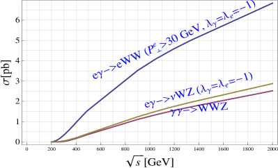
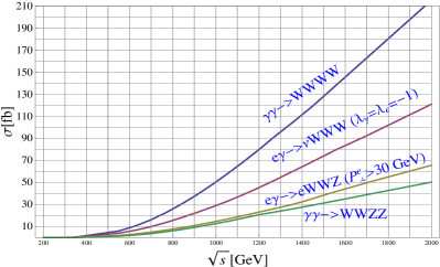
Figure 7: Cross sections for multiple production of gauge bosons, calculated with CalcHEP.

These cross sections are shown in Fig. 7. For processes $\mbox{$e\gamma\,$}\to eWW$, $\mbox{$e\gamma\,$}\to eWWZ$ we present cross sections for well observable transverse momenta of electrons ($p_{\bot e}>30$ GeV). Studying the dependence of these cross sections on the electron transverse momentum will allow to measure the electromagnetic form factor $W$ in the processes$\gamma\gamma^{*}\to WW$, $\to WWZ$ and separate the contribution of processes $Z^{*}\gamma\to WW$, $Z^{*}\gamma\to WWZ$ (at $p_{\bot e}>30$ GeV). The study of process $\mbox{$e\gamma\,$}\to\nu WZ$ allows to extract first information about subprocess $W^{*}\gamma\to WZ$.

$\bullet$ Hadron physics and QCD. Our understanding of hadron physics is twofold. We believe that we understand basic theory – QCD with its asymptotic freedom. However, the results of calculations in QCD can be applied to the description of data only with the aid some phenomenological assumptions (often verified by long practice). It results in badly controlled uncertainties in the description of data.

$\triangledown$ PLC is to some extent the hadronic machine with more pure initial state than LHC. Therefore, PLC can be used also for detailed study of high energy QCD processes like diffraction, total cross sections, odderon, etc. The results of such experiments can be confronted to theory with much lower uncertainty than the corresponding ones at the LHC.

$\triangledown$ The study of the photon structure function $W_{\gamma}$ (in $e\gamma\,$ mode) provides a unique test of QCD. This function can be written as the sum of point-like $W_{\gamma}^{pl}$ and hadronic $W_{\gamma}^{h}$ contributions. The hadronic part is similar to that for proton and it describes with similar phenomenology. In contrast, the point-like contribution $W_{\gamma}^{pl}$ is described without phenomenological parameters [19]. The ratio $W_{\gamma}^{h}/W_{\gamma}^{pl}$ decreases with $Q^{2}$ roughly as $(\ln Q^{2})^{-1/3}$. In the range of parameters accessible today the hadronic contribution dominates. With the growth of $Q^{2}$ at $e\gamma\,$ HE PLC the point-like part becomes dominant.

References

- [1] L.D. Landau, E.M. Lifshitz, Sow. Phys. 6 (1934) 244
- [2] V.M. Budnev, I.F. Ginzburg, G.V. Meledin and V.G. Serbo, Phys. Rep. 15C (1975) 181.
- [3] V.E. Balakin, V.M. Budnev, I.F. Ginzburg, Pis’ma ZhetF 11 (1970) 559 (ZhETF Lett. 11 (1970) 388); V.M. Budnev, I.F. Ginzburg, Phys. Lett. 37B (1971) 320; Sov. Yad. Fiz. 13 (1971) 353.
- [4] S. Brodsky, T. Kinoshita, H. Terazawa, Phys. Rev. Lett. 25 (1970) 972.
- [5] D. d’Enterria et al. PHOTON-2017 conference proceedings, arXiv:1812.08166
- [6] I.F. Ginzburg, G.L. Kotkin, V.G. Serbo and V.I. Telnov, ZhETF Pis’ma. 34 (1981) 514; Nucl. Instr. and Methods in Physics Research (NIMR) 205 (1983) 47; I.F. Ginzburg, G.L. Kotkin, S.L. Panfil, V.G. Serbo and V.I. Telnov, NIMR 219 (1983) 5.
- [7] B. Badelek et al. Int. J. Mod. Phys. A 19 (2004) 5097-5186; R.D. Heuer, … TESLA Technical Design Report, p. III DESY 2001-011, TESLA Report 2001-23, TESLA FEL 2001-05 (2001) p. 1–192 hep-ph/0106315; B.Badelek, … TESLA Technical Design Report, p. VI, chap.1 DESY 2001-011, TESLA Report 2001-23, TESLA FEL 2001-05 (2001) hep-ex/0108012, p.1-98; International Linear Collider. Technical Design report (2007-2010-2013); M. Harrison, M. Ross, N. Walker, ArXiv:1308.3726 [hep-ph]
- [8] V.I. Telnov. Nuclear and Particle Physics Proceedings 273 275 (2016) 219 224.
- [9] V.I. Telnov. ArXiv:1801.10471
- [10] P. Bambade et al. ArXiv:1903.01629 [hep-ex]
- [11] CLIC and CLICdp collaborations, CERN Yellow Rep. Monogr. 1802 (2018); CLIC and CLICdp Collaborations, A. Robson et al. ArXiv:1812.07987 [physics.acc-ph]; P. Roloff et al. ArXiv:1812.07986 [hep-ex]; J. de Blas et al. ArXiv:1812.02093 [hep-ph].
- [12] V.I. Telnov, NIMR A 472 (2001) 280-290.
- [13] I.F. Ginzburg, G.L. Kotkin. Photon 2009 (2009); I.F. Ginzburg. ArXiv:0912.4841 [hep-ph].
- [14] I.F. Ginzburg, G.L. Kotkin, Eur. Phys. J. C 13 (2000) 295
- [15] I.F. Ginzburg, G.L. Kotkin, S.L. Panfil, V.G. Serbo. Nucl. Phys. B 228 (1983) 285 – 300. (E: B 243 (1984) 550).
- [16] V.I. Telnov (2013), private communication.
- [17] A. Abada et al.,Eur. Phys. J. C79 (2019) 474
- [18] I.F. Ginzburg, V.A.Ilyin, A.E.Pukhov, V.G.Serbo, S.A.Shichanin. Rus. Yad. Fiz. 56 (1993) 57–63.
- [19] E. Witten. Nucl. Phys. B 120 (1977) 189.