A Distributed Model-Free Algorithm for Multi-hop Ride-sharing using Deep Reinforcement Learning

Abstract

The growth of autonomous vehicles, ridesharing systems, and self driving technology will bring a shift in the way ride hailing platforms plan out their services. However, these advances in technology coupled with road congestion, environmental concerns, fuel usage, vehicles emissions, and the high cost of the vehicle usage have brought more attention to better utilize the use of vehicles and their capacities. In this paper, we propose a novel multi-hop ride-sharing (MHRS) algorithm that uses deep reinforcement learning to learn optimal vehicle dispatch and matching decisions by interacting with the external environment. By allowing customers to transfer between vehicles, i.e., ride with one vehicle for sometime and then transfer to another one, MHRS helps in attaining 30% lower cost and 20% more efficient utilization of fleets, as compared to the ride-sharing algorithms. This flexibility of multi-hop feature gives a seamless experience to customers and ride-sharing companies, and thus improves ride-sharing services.

I Introduction

I-A Motivation

As the adoption of autonomous vehicles becomes more widespread, the need for ride-sharing and carpooling transportation will become even more prominent. Autonomous driving could lead to fewer accidents, fewer traffic deaths, greater energy efficiency, and lower insurance premiums [2, 3, 4]. It is estimated that savings with autonomous vehicles for the United States alone will be around $1.3 trillion [5]. Carmakers race to develop self-driving cars to use in fleets of robo-taxis to tap into the potentially lucrative new market. While ride-sharing (joint travel of two or more passengers in a single vehicle) has long been a common way to share the costs and reduce the congestion, it remains a nook transportation option with limited route choice and sparse schedules (only few rides per route). This work explores the benefits of allowing customers to transfer between vehicles to further improve the ride-sharing services.

Multi-hop ride-sharing (MHRS) plays a crucial role in revolutionizing the transport experience in ride-sharing and logistics transportation [6, 7, 8]. With the advancement of self-driving vehicle technology and proliferation of ride-sharing apps (e.g., Uber and Lyft), optimal distributed dispatching of vehicles is essential to minimize the supply-demand mismatch, reduce the waiting time of customers, reduce the travel cost, and utilize the fleet effectively. Also, multi-hop ride-sharing is a more competitive and reliable mode of transportation in terms of time and cost when compared with other modes of transport such as trains and buses [9, 10]. However, hopping and dispatch decisions over a large city for carpooling requires instantaneous decisions for thousands of drivers to serve the ride requests over an uncertain future-demand. Moreover, the dispatch decision for each vehicle could be time consuming, exacerbating the uncertainty of the optimization over a dynamically changing demand. We note that vehicle can only be dispatched if it is not fully occupied, and the travel time of a passenger, if any, within the vehicle should be minimized. Thus, the dispatch decision depends on the future potential trip requests which are uncertain in nature. Yet, realistic models are necessary to assess the trade-offs between possibly conflicting interests, minimizing the un-served ride requests, waiting time per request, total trip times of passengers, and the total trip distance of every vehicle.

One of the necessary components for a successful dynamic MHRS system is an efficient optimization techniques that matches drivers and riders in real-time. However, the majority of work in this domain (e.g., [11, 12, 13]) requires pre-specified model for demand prediction, user’s utilities for waiting times and travel times, and cost functions governing the cars’ total trip distance. These impact the decisions of route planning for the vehicles in real-time. Thus, a model based approach is unable to consider all the intricacies involved in the optimization problem. Further, a distributed algorithm is preferable where each vehicle can take its own decision without coordinating with the others. This paper aims to consider a model-free distributed approach for ride-sharing with carpooling with possible passenger transfer from one vehicle to another one. Our approach can adapt to the changing distributions of customer arrivals, the changing distributions of the active vehicles, the vehicles’ locations, and user’s valuations for the total travel time. The tools from deep reinforcement learning [14] are used for this dynamic modeling, where the vehicle dispatching is dynamically learned using the deep neural network, based on which the action is chosen with the Q-learning strategy.

I-B Related Work

Multi-hop ride-sharing poses myriad challenges that need to be addressed for efficient ride platforms services [6, 7, 15]. While fleet management and ride-sharing problems have been widely studied, most of the approaches in the literature are model-based, see [16, 17, 18, 19, 20, 8, 21] and the references therein. In such models, pickup request locations, travel time, demand prediction, route decisions, and destinations are assumed to follow certain distributions and then propose dispatching policies that would improve the performance [22, 23]. Using realistic data from ride-sharing services, the authors in [24] have modeled the customer requests and their variations over service area using a graph. The temporal/spatial variability of ride requests and the potentials for ride-pooling are captured. In [25], a matching algorithm based on the utility of the desired user is proposed. However, the proposed approach is a model-based that lacks adaptability and thus becomes impractical when the number of vehicles is very large, which is the scenario in our setting.

Recently, different approaches for dispatching vehicles and allocating transportation resources in modern cities are investigated. In [17], an optimal policy for autonomous vehicles is proposed, which considers both global service fairness and future costs. Yet, idle driving distance and real-time GPS information are not considered. In [26, 27], scheduling temporal-based methods are developed to reduce costs of idle cruising, however, the proposed algorithm does not utilize the real-time location information. Minimizing the total customer waiting time by concurrently dispatching multiple taxis and allowing taxis to exchange their booking assignments is investigated in [28]. Several studies in the literature, e.g., [29, 30, 31, 32], have shown that learning from past taxi data is possible. Thus, taxi fleet management and minimizing both waiting-time for passengers and idle-time for drivers can be obtained. In [31], authors used DQN for dynamic fleet management. Using realistic data, distributed DQN based approaches have shown to outperform the centralized solutions. This work is extended to accommodate the ride-sharing scenarios in [33]. In this paper, we generalize these models and consider a multi-hop ride-sharing system where a rider can reach a destination via a number of transfers (hops) and at the same time one or more passengers can share a single vehicle. With MHRS, the availability and range of the rideshare service increase, and also the total travelled vehicular miles can decrease.

I-C Our Contribution

In this paper, we propose a distributed model-free multi-hop ride-sharing algorithm for (i) dispatching vehicles to locations where future demand is anticipated, and (ii) matching vehicles to customers. We provide an optimized framework for vehicle dispatching that adopts deep reinforcement learning to learn the optimal policies for each vehicle individually by interacting with the external environment. Our approach allows customers to have one (or more) hops along the way to the destination. We note that customers who accept to have hop(s) along their paths to destination may experience a slightly longer time than direct path. However, this incurred time could be compensated by giving incentives to the customers (e.g., lower payment rate) to opt for the carpooling with multi-hop. Our results show a small increase in the total trip times as compared to the rid-sharing scenario (see Figure 1 and its description for further details).

Different from the majority of existing model-based approaches, we do not need to accurately model the system (so we call it model-free), rather, we use deep reinforcement learning technique in which each vehicle solves its own double deep Q-network (DDQN) problem in a distributed manner without coordination with cars in its vicinity. By doing so, a significant reduction in the complexity is obtained. To the best of our knowledge, this work is the first to cast the MHRS problem to a reinforcement learning problem. We aim to optimally dispatch the vehicles to different locations in a service area as to minimize a set of performance metrics including customers waiting time, extra travel time due to participating in MHRS and idle driving costs. Using real-world dataset of taxi trip records in New York City, our extensive simulation results show that, with the same overhead time as DeepPool [33], i.e., model-free algorithm for ride-sharing, passengers can complete their trips with $\sim 30\%$ lower costs. Further, MHRS can achieve upto $\sim 99\%$ accept rates, and thus minimizes the supply-demand mismatch. In addition, MHRS algorithm also helps reduce both waiting time and (idle) cruising time by $\sim 40\%$, with $\sim 20\%$ better utilization rate of vehicles.

I-D Organization

This paper is organized as follows. Section II explains the problem and present an example for MHRS and distinguishes it from ridesharing problem. In addition, the used notations and performance metrics used in this paper are briefly explained. Section III explains the proposed MHRS framework and describes the main components in the system design. In addition, a distributed version of our algorithm is further presented in this section. Section IV presents the simulator design and the evaluation results. It also highlights the main findings out of this work. Section V concludes the paper and gives possible venues for promising directions and future research.

II Problem Statement

We consider a MHRS scenario where customers can complete their trips in multiple hops. We develop an algorithm that dispatches vehicles to either pick-up passengers from their pickup and/or hop locations or to serve potential customers in the dispatched zones. The vehicle location, capacity, next destination, and number of passengers, etc. can be tracked in real time, thanks to mobile internet technologies. Without loss of generality, we consider the New York City area as our area of operation. The area is divided into multiple non-overlapping zones (or regions), each of which is $1$ square mile. This allows to discretize the area of operation and thus makes the action space (i.e, where to dispatch the vehicles) tractable.

II-A Multi-hop Example

Consider a simple multi-hop ride-sharing scenario as depicted in Figure 1. In this figure, both Rider $1$ and Rider $2$ want to go to the Central Park, NY. However, Rider $1$ and Rider $2$ are in different zones. Rider $1$ is in zone $A$, while Rider $2$ is in zone $C$. Since zone $B$ lies along the route of both Riders, Zone $B$ can be a hop zone, where one vehicle (say Vehicle $1$) can drop its passenger and join the another vehicle (Vehicle $2$). Here, Rider $1$ initially gets into the nearest vehicle (Vehicle $1$) and Rider 2 gets into Vehicle $2$. Vehicle $1$ drops rider 1 at zone $B$. As Vehicle $2$ reaches the hop zone (zone $B$), it picks up Rider $1$ and drops both at their destination, i.e., Central Park. As shown in the figure, $x$ represents the distance between zone $A$ and zone $B$, $y$ represents the distance between zone $B$ and Central Park, and $z$ is the distance between zone $B$ and zone $C$. We define the effective distance of Vehicle $2$, $D_{2}$, which gives the effective distance traveled by Vehicle $2$, as follows:

$$D_{2}=\frac{z+y+y}{z+y}=1+\frac{y}{z+y}$$ (1)

Thus, effective distance is formally defined as the ratio of total distance covered if no hoping and sharing was allowed to the total distance covered when hoping and sharing is allowed. We note that efficient packing of vehicles allows for less distance traveled by the vehicles in completing service of same number of requests. The multi hop scenario shown in Figure 1 reduces the traffic that goes from Zone $B$ to the Central Park. Further, MHRS allows vehicles to be free more frequently and thus can improve the accept rate of ride requests as in our example Vehicle $1$ is free after dropping Rider $1$ and can serve new customers accordingly.

Figure 1: A schematic illustrating the MHRS in a simple ride matching scenario. There are two vehicles (Vehicle $1$ and Vehicle $2$) and two ride requests (Ride $1$ and Ride $2$) at zones $A$ and $B$, respectively. Zone $B$ repesents at ”hop” zone where one passenger changes/transfers to another vehicle in zone $B$.

Figure 2: A schematic to illustrate the multi hop ride-sharing routing in a region graph, consisting of 13 regions, $A$ to $M$. There are five ride requests and four vehicles. The locations of both customers and vehicles are shown in the figure above. The zone ’F’ (colored in blue with a square shape) is the hop zone. The red dotted line shows the path of Vehicle 2 and green dotted line shows the path of Vehicle 3 in the multi-hop ride-sharing scenario.

II-B MHRS, Ride-sharing, and No-ride-sharing Scenarios

Figure 2 highlights the differences between different scenarios include: ride-sharing with multi-hop, ride-sharing with no-hops, and the case where only one rider per vehicle is allowed (no ride-sharing case). The figure shows the locations of vehicles and the passengers at a given time. Riders 1, 4 and 5 want to go to the Central Park, NY, while Riders 2 and 3 want to go to the Times Square, NY. There can be a scenario where Vehicle 2 takes Rider 1, and Vehicle 3 takes Rider 4 to the Central park. Further, vehicle 1 takes Rider 2 and Vehicle 4 takes Rider 3 to Times Square. In this case, no ride-sharing is involved and thus four vehicles are used to serve part of the demand. Since no more vehicles are available, Rider 5 request deemed rejected. We now consider a scenario where Vehicle 2 can serve Rider 1 (due to its proximity to Rider 1) and Vehicle 3 serves Riders 4 and 5. Vehicle 1 serves Rider 2 and Vehicle 4 serves Rider 3. In this case, ride-sharing allows efficient use of vehicles, thus no request is rejected. Still, there is a room for improvement through multi-hop ride-sharing. In such settings, Vehicle 2 picks-up Rider 1 from zone $D$ and drops Rider 1 at zone $F$ (i.e., a hop zone). Then, Vehicle 3 takes Rider 1, Rider 4 and Rider 5 to the Central Park (see the green dashed-line in Figure 2). In addition, Vehicle 2 moves from zone $F$ to zone $E$ to pick up Rider 2 and then picks up Rider 3 a long its way to the Times square, NY (the red dotted-line in Figure 2). In this case, only 2 vehicles are used to fulfill the demand. We note that under MHRS scenario, the non-used vehicles (Vehicle $1$ and Vehicle $4$) are free and able to serve other customers and thus improve the acceptance rate of ride-sharing systems.

From the proceeding discussion, we observe that MHRS leads to better utilization of vehicles, reduced travel cost due to sharing the cost by passengers, and reduced traffic congestion since less number of vehicles are used to serve the user’s demand. Since traffic is reduced, pollution could be also mitigated. Moreover, since fewer number of vehicles are used, the incurred fuel cost is reduced, which results in less cost for customers.

II-C Model Parameters and Notation

We use the following notations in our paper to define state, supply and demand. We use $i\in\{1,2,3,\ldots,M\}$ for the zones. The number of vehicles is taken as $N$. We optimize the multi hop system on $T$ time slots, where one time slot has length $\Delta t$. The vehicles take decisions at each time slot $\tau=t_{0},t_{0}+1,t_{0}+2,\cdots,t_{0}+T$, where $t_{0}$ is the current time slot. Let the number of available vehicles at region $i$ at time slot $t$ be ${v}_{t,i}$. A vehicle is marked as available if at least one of its seats is vacant. A vehicle is marked unavailable if it is completely full or does not consider taking an extra passenger. We can only dispatch those vehicles which are available. Vehicle $v$ has a maximum capacity of $C_{v}$ passengers. We take the number of requests at zone $i$ at time $t$ as ${d}_{t,i}$. $d_{t,\widetilde{t},i}$ is the number of vehicles that are not available at time $t$ but will drop-off a passenger(s) at zone $i$ and then become available at $\widetilde{t}$. We can estimate the $d_{t,\widetilde{t},i}$ using the estimated time of arrival (ETA) model [33]. We use $\bm{X}_{t}=\{\bm{x}_{t,1},\bm{x}_{t,2},\ldots,\bm{x}_{t,N}\}$ to denote the vehicles status at time $t$. $\bm{x}_{t,k}$ is a vector which consists of the current zone of vehicle $k$, available vacant seats, the time at which a passenger is picked up, and destination zone of each passenger. Using this information, we can also predict the time slot at which the unavailable vehicle $v$ will be available, $d_{t,\widetilde{t},i}$. Thus, for a set of dispatch actions at time $t$, we can predict the number of vehicles in each zone for $T$ time slots ahead, denoted by $\bm{V}_{t:t+T}$. We use ${hop}_{l,i,p}$ to denote the passenger $l$ hopped down at zone $i$, and $p$ denotes the $p^{th}$ hop of the passenger. We can improve upon our dispatching policies by estimating the demand in every zone through historical weekly/daily distribution of trips across zones [34]. We use $\bm{D}_{t:T}=\left(\overline{\bm{d}}_{t},\ldots,\overline{\bm{d}}_{t+T}\right)$ to denote the predicted future demand from time $t_{0}$ to time $t+T$ at each zone. Combining this data, the environment state at time $t$ can be written as $\bm{s}_{t}=\left(\bm{X}_{t},\bm{V}_{t:t+T},\bm{D}_{t:t+T}\right)$. Note that when a passenger’s request is accepted, we will append the user’s expected pick-up time, the source, and destination to $\bm{s}_{t}$.

II-D Objective

The objective of this paper is to optimally dispatch the vehicles to various locations and achieve these motives: a) ensure minimum waiting-time and dispatch/idle time for passengers and vehicles, respectively, b) minimize the gap between the supply and demand, c) minimize the number of used vehicles to serve the demand, d) minimize the number of hops (or transfers) for customers e) minimize the extra travel time for a customer for a given trip due to hops, and f) minimize the fuel consumption for each vehicle.

The metrics mentioned above will be explained in detail mathematically in the subsequent sections. We can associate different weights with these metrics. These weights help in deciding which metrics should be given more importance over others. For example, we can assign more weight to accept rate if we want to ensure high overall accept rate for the trips.

For every time step, the agent takes an action, in our case the vehicles choose to be dispatched to the zones where future demand is anticipated. The agent (i.e., vehicle) receives a reward based on the action taken. Ideally, the agent takes the actions that would maximize its expected discounted future reward, i.e.,

$$\sum_{k=t}^{\infty}\eta^{k-t}\bm{r}_{k}(\bm{a}_{t},\bm{s}_{t}),$$ (2)

where $\eta<1$ is a time discounting factor. In the context of this paper, the reward $\bm{r}_{k}(.)$ is defined as a weighted sum of different performance components that best capture the motive of our system as mentioned above. Since the number of vehicles is limited, it is likely that some rides may not be served, so we minimize the supply and demand gap. Since we want to motivate sharing and hopping but, at the same time, do not want the customer to have a bad experience, we minimize the overhead time and the number of hops per customer. In addition, we aim to minimize the wait time and idle cruising time to promote effective utilization of vehicles and smooth ride experience for the customer. The agent takes an action $\bm{a}_{t}$ based on the environment state $\bm{s}_{t}$ and receives the corresponding reward $\bm{r}_{t}$.

III Multi-Hop Ride-Sharing Framework Design

In this section, we present our framework to solve the MHRS problem. We propose a distributed model-free approach using DDQN, where the agent learns the best actions based on the reward it receives from the environment. It should be noted that the agent here refers to the vehicles, and our algorithm learns the optimal policy for each vehicle independently.

III-A Reward

The first component of the reward is to minimize the gap between the supply and demand for the agents/vehicles. Let $\bm{v}_{t,i}$ denote the number of available vehicles at time $t$ at zone $i$. Supply demand difference within time $t$ at zone $i$ can be written as $(\bm{v}_{t,i}-\bm{\overline{d}}_{t,i})$, i.e.,

$$\text{diff}^{(D)}_{t}=\sum_{i=1}^{M}\left(\overline{\bm{d}}_{t,i}-\bm{v}_{t,i}\right)^{+}$$ (3)

where $(.)^{+}=\text{max(0,.)}$. The second component of the reward is to minimize the dispatch time for the vehicles. Vehicles can be dispatched in two cases, either to serve a new request or to move to locations where a high demand is anticipated in the future. We note that only available vehicles can be dispatched. Dispatch time refers to the estimated travel time to go from the current zone to a particular zone, say zone $j$, i.e., $h^{n}_{t,j}$ if the vehicle $n$ is dispatched to zone $j$. Thus, for all available vehicles within time $t$, we wish to minimize the total dispatch time, $T^{(D)}_{t}$,

$$T^{(D)}_{t}=\sum_{n=1}^{N}\sum_{j=1}^{M}h^{n}_{t,j}u^{n}_{t,j}$$ (4)

where $u^{n}_{t,j}=1$ only if vehicle $n$ is dispatched to zone $j$ at time $t$. We seek to minimize the dispatch time sine drivers are consuming fuel without gaining revenue. Next, we want to minimize the extra travel time for every passenger (the third component). For vehicle $n$, rider $\ell$, at time $t$, we need to minimize $\delta_{t,n,\ell}=t^{\prime}+t_{t,n,\ell}^{(a)}-t_{n,\ell}^{(m)}$, where $t_{t,n,\ell}^{(a)}$ is the updated time the vehicle will take to drop off passenger $\ell$ because of change in route and/or addition of a rider from the time $t$. $t_{t,n,\ell}^{(m)}$ is the travel time that would have been taken if the passenger $\ell$ would not have shared the vehicle with any other passenger. Also, $t^{\prime}$ is the time elapsed after the user $\ell$ has requested its ride. Therefore, we can write

$$\bm{\Delta}_{t}=\sum_{n=1}^{N}\sum_{\ell=1}^{U_{n}}\delta_{t,n,\ell}$$ (5)

To ensure that the passengers do not have to go through any inconvenience (e.g., many hops a long the way to destination) in order to complete their trips, we minimize the number of hops a passenger has to make to complete the trip. Recall that $hop_{\ell,i,p}$ denote the passenger $\ell$ hopped down at zone $i$, and $p$ denotes the $p^{th}$ hop of the passenger $\ell$. Then,

$${H}_{\ell}=\sum_{i=1}^{M}\sum_{p=1}^{P}hop_{\ell,i,p}$$ (6)

Hence, the sum over all passengers $\ell$ at time $t$, gives the total number of hops of all customers at instant $t$, i.e., $\bm{H}_{t}=\sum_{\ell}H_{\ell}$. Lastly, the number of vehicles at any time $\bm{e}_{t}$ needs to be optimized to better utilize the vehicles usage (i.e., available resources), this can be written as

$$\bm{e}_{t}=\sum_{n=1}^{N}[\max\{\bm{e}_{t,n}-\bm{e}_{t-1,n},0\}]$$ (7)

where $e_{t,n}$ shows whether a vehicle has been occupied. We want to minimize the number of vehicles in the fleet that change their status from being inactive to active. This would ensure that the vehicles in the fleet are utilized efficiently. This would help in reducing the idle cruising time of the vehicles, hence would lead to better vehicle utilization.

Now that we have obtained our main objective equations, we can define the accumulated reward equation, for all vehicles, at time $t$ as follows:

$$\overline{r}_{t}=-[\beta_{1}\text{diff}^{(D)}_{t}+\beta_{2}T^{(D)}_{t}+\beta_{3}\bm{\Delta}_{t}+\beta_{4}\bm{e}_{t}+\beta_{5}\bm{H}_{t}]$$ (8)

The minus sign indicates we want to minimize those terms, and $\beta_{1},\beta_{2},\beta_{3},\beta_{4},\beta_{5}$ are weights and can be changed based on any specific objective we want to meet. For example, $\beta_{i}$ could be the cost per measure unit, e.g., cost per second. Moreover, we can increase $\beta_{4}$ if we decide our main goal to minimize the size of the fleet. Also, $\beta_{i},\forall i$, can be vehicle dependent (i.e., $\beta_{i,n},\forall i,n$) where each vehicle can choose its weights based on the drivers preference. We note that the reward is not an explicit function of the action. Through the model free approach, we learn the optimal relationship between action and reward by our algorithm.

We note that equation (8) gives the accumulated reward of all vehicles at time $t$ in a centralized manner. To solve the problem in a distributed fashion where each vehicle solves its own DDQN individually, we need to write the reward (and its related components) of every vehicle independent of other vehicles. In the next section, we provide the reward expression for each vehicle individually and show that by summing over all vehicles the total reward function is analogous to the objective function described in Section III.

III-B Distributed MHRS Framework

We build a simulator to train and evaluate our framework. We assume that a central unit is responsible for maintaining the states of all vehicles, e.g., current locations, destinations, occupancy state, etc. These states are updated in every time step based on the dispatching and assignments decisions. When needed, a vehicle $n$ communicates with the central unit to either request new information of other vehicles or update its own status. The goal of our distributed MHRS policy is to learn the optimal dispatch actions for each vehicle individually. Towards that goal, at every time slot $t$, vehicles decide $sequentially$ the next step (which zone to go) taking into consideration the locations of all other nearby vehicles in its vicinity. However, their current actions do not anticipate the future actions of other vehicles. We note that it is unlikely for two (or more) drivers to take actions at the same exact time since drivers know the location updates of other vehicles in real time, through the GPS for example. The advantage of MHRS policy stems from the fact that each vehicle can take its own decision without coordination with other vehicles. Next, we explain the state, reward and action.

III-B1 State

The state variables capture the environment status and thus affect the reward feedback of different actions. The state at time $t$ is captured by a three tuple $t$: $\left(\bm{X}_{t},\bm{V}_{t:t+T},\bm{D}_{t:t+T}\right)$. These elements are combined in one vector denoted as $\bm{s}_{t}$. When a set of new ride requests are generated, the MHRS engine updates its own data to keep track the environment status. The three-tuple state variables in $\bm{s}_{t}$ are pushed as an input to the neural network input layer to make a certain decision.

III-B2 Action

We denote the action of vehicle $n$ by $\bm{a}_{t,n}$. This action consists of two components –1) if the vehicle is partially filled it decides whether to serve the existing passengers or to accept new customer, and ii) if it decides to serve a new customer or the vehicle is totally empty, it decides the zone it should head (or hop) to at time slot $t$, which we denote by $u_{t,n,i}$. Here, $u_{t,n,i}=1$ if the vehicle decides to serve a new customer and/or head to zone $i$, otherwise it is $0$. Note that if vehicle $n$ is full it can not serve any additional customer. In contrast, if a vehicle decides to serve current customers, it opts the shortest optimal route for reaching the destinations of the users.

III-B3 Reward

We now represent the reward fully, and the weights which we put towards each component of the reward function for each vehicle if it is not full. The reward $r_{t,n}$ for vehicle $n$ at time slot $t$ in this case is given by

$$r_{t,n} =r(\bm{s}_{t,n},\bm{a}_{t,n})$$

$$=\beta_{1}b_{t,n}-\beta_{2}c_{t,n}-\beta_{3}\sum_{\ell=1}^{U_{n}}\delta_{t,n,\ell}$$

$$-\beta_{4}\max\{e_{t,n}-e_{t-1,n},0\}-\beta_{5}\underset{\ell\in\mathcal{L}_{t,n}}{\text{max}}\{\bm{H}_{\ell}\}$$ (9)

where $\beta_{i}$ is the weight for component $i$ in the reward expression. Note that $\bm{H}_{t,n}=\underset{\ell\in\mathcal{L}_{t,n}}{\text{max}}\{\bm{H}_{\ell}\}$. Further, $b_{t,n}$ denotes the number of customers served by vehicle $n$ at time $t$ while $c_{t,n}$ denotes the time taken by vehicle $n$ to hop or take a detour to pick up extra customers if the vehicle has available seats. $\delta_{t,n,\ell}$ denotes the additional time vehicle $n$ takes because of carpooling compared to the scenario if the vehicle would have served customer $\ell$ solely without any carpooling and/or hoping. Note that while taking the decision, the vehicle $n$ exactly knows the destination of the passenger. Note that when a user is added, the route is updated for dropping the passengers. $U_{n}$ is the total number of chosen customers for pooling at vehicle $n$ till time $t$. $\mathcal{L}_{t,n}$ contains the set of all customers assigned to vehicle $n$ at instant $t$. Note that both $U_{n}$ and $\mathcal{L}_{t,n}$ are not known a priori and will be adapted dynamically in the MHRS policy. These two quantities will also vary as the passengers being picked or dropped by the vehicle $n$. The last term captures the vehicle status where $e_{t,n}$ is set to one if empty vehicle $n$ becomes occupied (even if by one passenger), however, if an already occupied vehicles takes a new customer it is $0$. The intuition behind this reward term is that if an already occupied vehicle serves a new user, the congestion cost and fuel cost will be less rather than an empty vehicle serves the user. Note that if we make both $\beta_{3}$ and $\beta_{5}$ very large, we resort to the scenario where there is no carpooling. Since high $\beta_{3}$ indicates that passengers will not prefer detours to serve another passenger. Thus, the setting becomes similar to the one in [31]. Moreover, by setting $\beta_{5}$ to a very large value, our MHRS algorithm will resort to that of ride-sharing with no passenger transfer capability, which is similar to the algorithm presented in [33].

III-C Selection of Hop Zones

Hop zones are the zones where customers hop down from a vehicle and wait for the next vehicle to complete the rest of their trips. We start by dividing the city into 212 x 219 square grids. To run our DDQN algorithm, we further combine grids to form a new map of 41 x 43 square grids, preventing our action space from exploding. Every third intersection of zones in the horizontal and vertical direction is considered a hop zone. Since we want to make sure that the hop zones are in the busy area of the city and are not too closely placed, we consider only the zones with at least 10 ride requests in the day. Through this method, we obtain 148 hop zones in the whole New York city.

III-D MHRS Algorithm Description

In this section, we explain our proposed algorithm for MHRS in detail. The full algorithm is shown in Algorithm 1. We first construct the state vector $\bm{\varOmega}_{t,n}$, using the ride requests and available vehicles, which are extracted from real records (line 1). Then, we initialize the number of vehicles and generate some ride requests in each time step based on the real record in the dataset (see lines 2 to 5). Next, the agent determines the actions $\bm{a}_{t}$ using our MHRS algorithm and matches the vehicle to the appropriate ride request (or requests), lines 6 to 14. Every vehicle $n$ selects the action that maximizes its own reward, i.e., taking the argmax of the DDQN-network output. The output of the DDQN are the Q-values corresponding to every possible movement, while the input is the environment status governed by the vector $\bm{s}_{t}$. Note that each vehicle updates its status at the agent based on the chosen action (line 15). We note that the updates are performed sequentially so that vehicles can take other vehicles’ actions into account when making their own decisions. Nonetheless, each vehicle does not anticipate the future actions of other vehicles, thus limiting the coordination among them. Then, the vehicles traverse to the dispatched locations using the shortest path in the road network graph. The dispatched vehicles travel to target locations within the time estimated by our model (Section IV-B), see lines 18 to 23. The extra travel time $\delta_{t,n}$ and hop counter $H_{t,n}$ are updated as needed (lines 19-25).

Algorithm 1 MHRS Algorithm

1:Form a state vector $\bm{\varOmega}_{t,n}=\left(\bm{X}_{t},\bm{V}_{t:t+T},\bm{D}_{t:t+T}\right)$.

2:Initialize vehicles states $\bm{X}_{0}$ as location of first $N$ requests.

3:for $t\in$ Total time do

4:     Get all ride requests at time $t$

5:     Group all the requests assigned to the same hop zone

6:     for Each request group in time slot $t$ do

7:         Match a vehicle $n$ to serve the requests

8:         Update the vehicle capacity

9:         Update the pickup and destination for hop trips

10:         Calculate wait time and the number of passengers

11:         without any hops

12:         Calculate the dispatch time using ETA model

13:         Update the state vector $\bm{\varOmega}_{t,n}$.

14:     end for

15:     Send the state vector $\bm{\varOmega}_{t}$ to the Q network.

16:     Get the best dispatch action $\bm{a}_{t}$ for each agent from

17:     the network.

18:     for  all the available vehicles $n\in\bm{a}_{t}$  do

19:         Update $\bm{H}_{t,n}$, if needed, and update the current

20:         location of vehicle

21:         Find the shortest path to every dispatch location

22:         for every vehicle $n$.

23:         Estimate the travel time using the ETA model

24:         Update $\delta_{t,n}$, if needed, and generate the trajectory

25:         of vehicle $n$.

26:     end for

27:     Update the state vector $\bm{\varOmega}_{t+1}$.

28:end for

IV Simulator Setup and Evaluation

IV-A Setup and Initialization

Through extensive simulations, we show how MHRS algorithm works in real time scenario as compared to ride-sharing [33] and no ride-sharing [31] scenarios. We trained our algorithm using real world taxi trips in New York City for May 2016. Then, we tested our algorithm using the trip records of the first two weeks of June 2016 data. We divide the New York city into grids of size $41\times 43$, each grid has a an area of 800 x 800 m².

To initialize the environment, we run the simulation for $20$ minutes without dispatching the vehicles. Further, we set the number of vehicles to $N=5000$. The initial locations of these vehicles correspond to the first $5000$ ride requests. We set the maximum horizon to $T=30$ step and $\Delta t=1$ minute. We breakdown the reward and investigate the performance of the different policies. Further, unless otherwise stated, we set $\beta_{1}=5$, $\beta_{2}=1$, $\beta_{3}=3.5$, $\beta_{4}=0.05$, and $\beta_{5}=2$.

Recall that the reward function is composed of five different metrics, which we seek to minimize: (i) mismatch between supply and demand, (ii) dispatch time for vehicles, (iii) extra travel time because of ride-sharing and/or detouring for hops, (iv) number of used vehicles (resources), and finally (v) number of hops per customer. We note that the supply-demand mismatch is reflected in our simulation through the accept rate metric. This metric is computed as the number of ride accepts divided by the total number of requests per day. Recall that a request is deemed rejected if there is no vehicle in a range of $5km^{2}$, or no vehicle is available to serve the request. Also, the metric of idle time represents the time at which a vehicle is not occupied while still incurring gasoline cost and not gaining revenue. In addition, the waiting time is composed of two sub-components: the time from the ride request till the time at which the vehicle arrives to pick up the customer and the incurred wait time in hop zone(s), if any. Below, we explain our models to estimate the time of arrival, demand and our proposed DDQN architecture.

IV-B Estimated Time of Arrival (ETA) and Demand Prediction

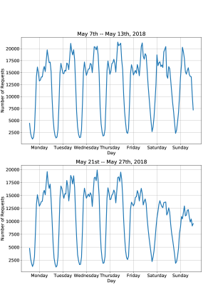
Figure 3: Demand pattern for two weeks in May 2018.

We use the New York City taxi data set [35] to build the ETA and demand prediction models. In the ETA model, we want to predict the expected travel time between two zones (two pairs of latitudes and longitudes). We split our data into 70% train and 30% test. We use day of week, latitude, longitude and time of days as our predictor variables and use random forest to predict the ETA. We obtain a root mean squared error (RMSE) of 3.4 on the test data.

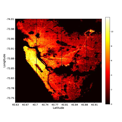
Figure 4: Demand Heat Map in New York City

For the demand prediction model, we predict the expected number of requests in a given zone for $15$ and $30$ minutes ahead. We plot in Figure 3 the weekly number of ride requests for two different weeks: May 7th-May 14th and May 21st-May 27th. We observe that both two weeks data exhibits the same daily behavior. In particular, both datasets experience daily periodicity with lower demand on the weekend, and thus the demand has a daily/weekly pattern that can be predicted. In Figure 4 we show the demand pattern in the form of a heat map. The New York city is plotted in the form of a rectangular grid of size 212 x 219. The brightest areas on the heat map, yellow zones, belong to the Manhattan area, where the trip demands are very high throughout the day.

We use convolutional neural networks for our demand predictions. The input to the network is 2 planes of 212 x 219. Each grid in the planes represents the ride request in that zone for the previous 2 time steps. In the network, we have 16 of 5x5 filters, 32 of 3x3 filters and finally one 1x1 filter. The output is a plane of 212x219, with each grid in the plane representing the demand in that zone in the next 30 minutes. The output of the demand prediction model will be used in the state in our model free algorithm. It should be further noted that we are not explicitly learning the transition probabilities from one state to another, which makes our approach model free.

IV-C Deep Q-Network Architecture

For the DDQN, we divide the New York City area map to obtain 41 x 43 grids. We do so to limit the action space of vehicles to $7$ grids vertically and horizontally. Thus the action space for each vehicle is 15 x 15 grid around its present location. The input to the deep Q network is the state of vehicles, supply and demand. Specifically, it consists of predicted requests in the next 15 minutes obtained from demand model, current location of each vehicle, future location of each vehicle in the next 15, and 30 minutes. The network architecture consists of 16 convolution layers of 5 x 5, 32 convolution layer of 3 x 3, 64 convolution layer of 3 x 3, 16 convolution layer of 1 x 1. All convolution layers have a rectifier non linearity activation. The output of the deep Q network is 15x 15 Q values, where each value corresponds to the reward a vehicle could get if dispatched to that particular zone.

Reinforcement learning becomes unstable for non linear approximations, hence we use experience replay to overcome this issue. We define a new parameter, $\alpha$ to address this issue. We memorize the experiences and randomly sample from these experiences to avoid correlation between immediate actions and experiences. The value of $\alpha$ is an indication of how frequently the target Q values are updated, indicating how much the agents are learning from their past experiences. In our case, we have taken $\alpha$ as 0.9

IV-D Evaluation and Results

We compare the results of our MHRS algorithm with two scenarios: no ride-sharing (No-RS) and ride-sharing (RS). No-RS means the vehicles are dispatched using DDQN policies but only one rider can occupy a vehicle at any given time. This policy is akin to that in [31], which we refer in our simulation comparisons as ”MOVI”. For the RS case, in addition to DDQN dispatch policies, more than one passenger can be assigned to one vehicle but no multi-hop is performed. This policy is proposed in [33], so-called DeepPool. In our MHRS policy, ridesharing is allowed and passengers could complete their trips in more than one hop.

Unless otherwise stated, we set up the simulator with 5000 vehicles. The time step was taken as one minute and the agents were trained on data of one month duration and tested on data of two weeks (first two weeks of June 2016). The initial location of the vehicles are corresponding to the locations of the first 5000 trips.

Figure 5: Accept rate versus the average number of hops.

Figure 6: Effective distance ratio versus number of hops.

Figure 7: Average idle time per request for different accept rate.

Figure 8: Average wait time per request for different accept rate.

Figure 9: Average used vehicles for different accept rate.

Figure 10: Average idle time for different number of vehicles.

Figure 7 plots the average accept rate versus the number of hops. We change the parameter $\beta_{5}$ to show the effect of hops on the accept rate. The values of $\beta_{5}$ used are - $2$, $1.9$, $1.8$, $1.7$, $1.6$, $1.5$ and $1.4$. Note that if a passenger is dropped at a hop zone and not served in $\delta_{t,n,\ell}$, this passenger request is deemed rejected. Since DeepPool and MOVI are not function of the number of hops, both have fixed acceptance rates at $0.95$ and $0.92$, respectively. We note that by $1.40$ hops, only $40\%$ of the total trips have $2$ hops. While the accept rate decreases as number of hops increases, our MHRS approach still performs the best as compared to both DeepPool and MOVI. This decrease of accept rate is due to the possibility for our algorithm to fail serving some of the passengers at the hop zones. In addition, some passengers complete their trips in more than one hop, thus making some vehicles available at the hop zones. Hence, vehicles get free more often as compared to when they had to travel long distances in one trip.

Figure 7 shows the effective distance ratio of vehicles (defined in (1)) versus the number of hops. We change the parameter $\beta_{5}$ to show the effect of hops on the effective distance. The values of $\beta_{5}$ used are - $2$, $1.9$, $1.8$, $1.7$ and $1.6$. Increasing effective distance with number of hops suggests that the vehicle is more efficiently packed as number of hops increases. Since only one passenger is assigned to a vehicle in MOVI, its effective distance is 1. It is evident that MHRS is efficient as compared to DeepPool since the former achieves better overall utilization of vehicles even when the number of hops is close to 1.

Figures 7, 10 and 10 plot the idle time, wait time and number of vehicles used respectively for different accept rates. We change the values of $\beta_{1}$ to obtain the figures. The values of $\beta_{1}$ used are - $5$, $7$, $8$, $9$ and $10$.

The idle time per vehicle is captured in Figure 7. Idle time is defined as total time when the cars are not serving any request divided by the total number of requests. This metric gives an indication on how much time a vehicle is burning extra fuel without serving any customer or gaining revenue. Clearly, MHRS leads to a significant decrease in the idle cruising time of vehicles. Small idle time would encourage incessant revenue generation for the taxi provider firms as well as quick fulfillment of customer demands (This can also be inferred from Figure 7).

Figure 10 shows that the wait time decreases as the accept rate increases. Wait time is defined as the average difference between the time of request for a passenger and the time when the passenger starts his/her ride. MHRS outperforms DeepPool and MOVI, and thus suggesting more than one hop allows customers to have sufficient vehicles in their vicinity and hence less waiting time on average. The number of used vehicles for different accept rate is shown in Figure 10. The number of used vehicles is defined as the average number of vehicles used to fulfill the requests. We note that MHRS needs fewer number fo vehicles as compared to DeepPool and MOVI. This indicates that MHRS contributes towards reduced fuel consumption and less traffic. Further, it leads not only to a constant circulation of supply but also helps in minimizing the fleet size and maintenance cost.

Figure 11: Average accept rate for different number of vehicles.

Figure 12: Distribution of customer trips with and without hops for our proposed MHRS algorithm.

The effect of varying the number of vehicles on waiting time and idle time is captured in Figures 10 and 11. We only change the number of vehicles and set our parameters as - $\beta_{1}=5$, $\beta_{2}=1$, $\beta_{3}=3.5$, $\beta_{4}=0.05$, and $\beta_{5}=2$. Intuitively, as the number of vehicles increases, the idle time increases since more vehicles will compete the existing passengers and further cruise searching for potential customers. However, our approach of MHRS still achieves the lowest idle time even in the regime of low number of vehicle. While DeepPool allows pooling customers together, it remains a nook option with limited route choice and few rides per route can be pooled. This highlights the importance of allowing customers to transfer vehicles to further improve the quality of experience of passengers.

Figure 11 plots the accept rate for different number of vehicles. The gain of the MHRS over both DeepPool and MOVI policies is remarkable even for low number of vehicles, which highlights the benefits of ride-sharing with passenger transfer capabilities in meeting customer demand at small travel time overhead. We observe that both DeepPool and MOVI achieve higher accept rate as the number of vehicle increase. This is because more vehicles can be dispatched. Further, DeepPool algorithm can serve more customers using a single car by better utilizing the passengers proximity. However, this comes at an additional increased in the idle time of vehicles as depicted in Figure 10. By allowing passengers transfer, vehicles can pool even more customers which results in increasing the accept rate of passengers.

The distribution of customer trips that encounter hops/transfers during their paths to destination is shown in Figure 12. This figure also shows the total number of customer trips without hops (i.e., total number of passenger trips that reach their destinations using a single vehicle). We can see that approximately $50\%$ of the total trips involve customer transfers. By seeing this figure along with Figures 7–7, we conclude that most of the passengers experience only one transfer/hop at most. Hence, with only one transfer (going from one direct trip to two hops) on $50\%$ of the total trips, we notice significant reductions in customers waiting times, vehicle idle times, and the total number of used vehicle. This shows that it would be sufficient to search only for one transfer since shared rides with two (or more) hops does not give significantly better performance, on an average.

V Conclusion and Future Work

We have looked at the problem of multi-hop ride-sharing, where passengers can be dropped one or more times before reaching their destinations. We have proposed an efficient distributed model-free algorithm for dispatching and matching policies where reinforcement learning techniques are used to to learn the optimal decisions for each vehicle individually. We have observed better accept rates, more efficient utilization of vehicles, a constant revenue cycle and reduced prices for customers. Further, we have seen a significant improvement in waiting time, idle time, and the number of used vehicles when going from one hop to two hops, but we have not seen any considerable changes when further increasing the hop count. This indicates that searching for shared rides with three (or more) hops does not give significantly better results, on an average. Surprisingly, a negligible improvement is noticed for more than two hops.

As a future research, utilizing the interaction between vehicles in a multi-agent reinforcement learning settings is a nice future direction. Further, optimal incentive techniques to influence passengers to opt for the MHRS is another promising research area. Lastly, as a promising alternative to the inefficient traditional package delivery techniques, MHRS systems represent a potential delivery capability through ridesharing within an urban environment. By allowing the passengers and the packages with similar itineraries and time schedules to share one vehicle, the delivery cost and time can be reduced significantly.

References

- [1] A. Singh, A. O. Al-Abbasi, and V. Aggarwal, “A reinforcement learning based algorithm for multi-hop ride-sharing: Model-free approach,” in Neural Information Processing Systems (Neurips) Workshop, Dec 2019.
- [2] T. Litman, Autonomous vehicle implementation predictions. Victoria Transport Policy Institute Victoria, Canada, 2017.
- [3] J. M. Anderson, K. Nidhi, K. D. Stanley, P. Sorensen, C. Samaras, and O. A. Oluwatola, Autonomous vehicle technology: A guide for policymakers. Rand Corporation, 2014.
- [4] P.-L. Blyth, M. N. Mladenovic, B. A. Nardi, H. R. Ekbia, and N. M. Su, “Expanding the design horizon for self-driving vehicles: Distributing benefits and burdens,” IEEE Technology and Society Magazine, vol. 35, no. 3, pp. 44–49, 2016.
- [5] A. Kearney, “How automakers can survive the self-driving era,” Retrieved November, vol. 14, p. 2017, 2016.
- [6] F. Drews and D. Luxen, “Multi-hop ride sharing,” in Sixth annual symposium on combinatorial search, 2013.
- [7] T. Teubner and C. M. Flath, “The economics of multi-hop ride sharing,” Business & Information Systems Engineering, vol. 57, no. 5, pp. 311–324, 2015.
- [8] Y. Chen, D. Guo, M. Xu, G. Tang, T. Zhou, and B. Ren, “Pptaxi: Non-stop package delivery via multi-hop ridesharing,” IEEE Transactions on Mobile Computing, 2019.
- [9] B. Coltin and M. Veloso, “Ridesharing with passenger transfers,” in 2014 IEEE/RSJ International Conference on Intelligent Robots and Systems. IEEE, 2014, pp. 3278–3283.
- [10] T. Teubner and C. M. Flath, “The economics of multi-hop ride sharing,” Business & Information Systems Engineering, vol. 57, no. 5, pp. 311–324, Oct 2015.
- [11] M. Zhu, X.-Y. Liu, F. Tang, M. Qiu, R. Shen, W. W. Shu, and M.-Y. Wu, “Public vehicles for future urban transportation.” IEEE Trans. Intelligent Transportation Systems, vol. 17, no. 12, pp. 3344–3353, 2016.
- [12] N. Agatz, A. Erera, M. Savelsbergh, and X. Wang, “Optimization for dynamic ride-sharing: A review,” European Journal of Operational Research, vol. 223, no. 2, pp. 295–303, 2012.
- [13] B. N. Greenwood and S. Wattal, “Show me the way to go home: An empirical investigation of ride-sharing and alcohol related motor vehicle fatalities.” MIS quarterly, vol. 41, no. 1, pp. 163–187, 2017.
- [14] V. Mnih, K. Kavukcuoglu, D. Silver, A. A. Rusu, J. Veness, M. G. Bellemare, A. Graves, M. Riedmiller, A. K. Fidjeland, G. Ostrovski et al., “Human-level control through deep reinforcement learning,” Nature, vol. 518, no. 7540, p. 529, 2015.
- [15] K. M. H. Sonet, M. M. Rahman, S. R. Mehedy, and R. M. Rahman, “Shary: a dynamic ridesharing and carpooling solution using advanced optimised algorithm,” International Journal of Knowledge Engineering and Data Mining, vol. 6, no. 1, pp. 1–31, 2019.
- [16] H. Zheng and J. Wu, “Online to offline business: urban taxi dispatching with passenger-driver matching stability,” in Distributed Computing Systems (ICDCS), 2017 IEEE 37th International Conference on. IEEE, 2017, pp. 816–825.
- [17] R. Zhang and M. Pavone, “Control of robotic mobility-on-demand systems: a queueing-theoretical perspective,” The International Journal of Robotics Research, vol. 35, no. 1-3, pp. 186–203, 2016.
- [18] S. Ma, Y. Zheng, and O. Wolfson, “Real-time city-scale taxi ridesharing,” IEEE Transactions on Knowledge and Data Engineering, vol. 27, no. 7, pp. 1782–1795, 2015.
- [19] R. Gopalakrishnan, K. Mukherjee, and T. Tulabandhula, “The costs and benefits of sharing: Sequential individual rationality and sequential fairness,” arXiv preprint arXiv:1607.07306, 2016.
- [20] X. Bei and S. Zhang, “Algorithms for trip-vehicle assignment in ride-sharing,” in Thirty-Second AAAI Conference on Artificial Intelligence, 2018.
- [21] N. Masoud and R. Jayakrishnan, “A decomposition algorithm to solve the multi-hop peer-to-peer ride-matching problem,” Transportation Research Part B: Methodological, vol. 99, pp. 1–29, 2017.
- [22] B. Coltin, “Multi-agent pickup and delivery planning with transfers,” 2014.
- [23] B. J. Coltin and M. Veloso, “Towards ridesharing with passenger transfers,” in Proceedings of the 2013 international conference on Autonomous agents and multi-agent systems. International Foundation for Autonomous Agents and Multiagent Systems, 2013, pp. 1299–1300.
- [24] A. Jauhri, B. Foo, J. Berclaz, C. C. Hu, R. Grzeszczuk, V. Parameswaran, and J. P. Shen, “Space-time graph modeling of ride requests based on real-world data,” in Workshops at the Thirty-First AAAI Conference on Artificial Intelligence, 2017.
- [25] V. M. de Lira, V. C. Times, C. Renso, and S. Rinzivillo, “Comewithme: An activity-oriented carpooling approach,” in 2015 IEEE 18th International Conference on Intelligent Transportation Systems. IEEE, 2015, pp. 2574–2579.
- [26] J. Yang, P. Jaillet, and H. Mahmassani, “Real-time multivehicle truckload pickup and delivery problems,” Transportation Science, vol. 38, no. 2, pp. 135–148, 2004.
- [27] D. Bertsimas, P. Jaillet, and S. Martin, “Online vehicle routing: The edge of optimization in large-scale applications,” Operations Research, 2019.
- [28] K. T. Seow, N. H. Dang, and D.-H. Lee, “A collaborative multiagent taxi-dispatch system,” IEEE Transactions on Automation Science and Engineering, vol. 7, no. 3, pp. 607–616, 2010.
- [29] F. Miao, S. Han, S. Lin, J. A. Stankovic, D. Zhang, S. Munir, H. Huang, T. He, and G. J. Pappas, “Taxi dispatch with real-time sensing data in metropolitan areas: A receding horizon control approach,” IEEE Transactions on Automation Science and Engineering, vol. 13, no. 2, pp. 463–478, 2016.
- [30] D. Zhang, T. He, S. Lin, S. Munir, and J. A. Stankovic, “Taxi-passenger-demand modeling based on big data from a roving sensor network,” IEEE Transactions on Big Data, vol. 3, no. 3, pp. 362–374, 2017.
- [31] T. Oda and C. Joe-Wong, “Movi: A model-free approach to dynamic fleet management,” in IEEE INFOCOM 2018-IEEE Conference on Computer Communications. IEEE, 2018, pp. 2708–2716.
- [32] T. Oda and Y. Tachibana, “Distributed fleet control with maximum entropy deep reinforcement learning,” in NIPS 2018 Workshop MLITS, 2018.
- [33] A. Alabbasi, A. Ghosh, and V. Aggarwal, “DeepPool: Distributed model-free algorithm for ride-sharing using deep reinforcement learning,” IEEE Trans. Intelligent Transportation Systems (to appear), 2019.
- [34] D. C. Wyld, M. A. Jones, and J. W. Totten, “Where is my suitcase? rfid and airline customer service,” Marketing Intelligence & Planning, vol. 23, no. 4, pp. 382–394, 2005.
- [35] NYC, “NYC Taxi & Limousine Commission-Trip Record Data- NYC.gov,” www.nyc.gov, 2018.