Portfolio Optimization with Expectile and Omega Functions

Abstract.

This paper proves equivalences of portfolio optimization problems with negative expectile and omega ratio. We derive subgradients for the negative expectile as a function of the portfolio from a known dual representation of expectile and general theory about subgradients of risk measures. We also give an elementary derivation of the gradient of negative expectile under some assumptions and provide an example where negative expectile is demonstrably not differentiable. We conducted a case study and solved portfolio optimization problems with negative expectile objective and constraint.

©2019 IEEE. Personal use of this material is permitted. Permission from IEEE must be obtained for all other uses, in any current or future media, including reprinting/republishing this material for advertising or promotional purposes, creating new collective works, for resale or redistribution to servers or lists, or reuse of any copyrighted component of this work in other works.

1. Introduction

In this paper, portfolio optimization is the task of maximizing the expected return of a portfolio subject to the risk of the portfolio not exceeding a prespecified level. Formally, let $\xi=(\xi_{1},\dots,\xi_{n})$ be a vector containing random variables representing the returns of $n$ financial instruments. Let $x=(x_{1},\dots,x_{n})\in\mathbb{R}^{n}$. The random return of the portfolio is given by $\xi^{\intercal}x$. The decision variable $x_{i}$ represents position being invested in the $i$-th instrument. Let us denote the risk measure of interest by $R$. We investigate two single-stage stochastic optimization problems,

$$\max E[\xi^{\intercal}x]\quad\text{subject to}\quad R(\xi^{\intercal}x)\leq b,\ x\in V\in\mathbb{R}^{n}\;\text{ and}$$

$$\min R(\xi^{\intercal}x)\quad\text{subject to}\quad E[\xi^{\intercal}x]\geq r,\ x\in V\in\mathbb{R}^{n}\;,$$

where $V\in\mathbb{R}^{n}$ is a convex set of feasible portfolios.

This paper considers two closely related risk measures, negative expectile and omega. Expectiles are asymmetric generalizations of expected value introduced by newey1987asymmetric and defined by (3). When $q\leq\frac{1}{2}$, negative level-$q$ expectiles satisfy the conditions of a coherent risk measure in the sense of artzner1999coherent. Section 4 of this paper shows that for $q<\frac{1}{2}$ the level-$q$ negative expectile is strictly expectation bounded (i.e. averse) as defined by rockafellar2006generalized. Moreover, negative expectile is elicitable, that is there exists a consistent way of comparing the quality of procedures that predict its value [ZiegelZiegel2016]. Indeed, Bellini2019 have suggested a procedure for testing the accuracy of an expectile forecasting model. A conditional version of expectile naturally generalizing conditional expectation has also been developed BELLINI2018117.

In addition to this list of desirable theoretical properties, bellini2017risk offer the following intuitive motivation for the use of negative expectile as a measure of risk for portfolio optimization. Value at risk is a commonly used risk measure and can be given by (1) employing the concept of acceptance sets. The same reformulation can be given to negative expectile as in (2).

(1) $$\text{VaR}_{\alpha}(X)=\inf\{m\in\mathbb{R}\ |\ P(X+m>0)\geq\frac{1-\alpha}{\alpha}P(X+m\leq 0)\}$$

(2) $$R_{q}(X)=\inf\{m\in\mathbb{R}\ |\ E[(X+m)_{+}]\geq\frac{1-q}{q}E[(X+m)_{-}]\}$$

So if VaR represents the smallest amount we need to add to the random return such that the probability of a gain is $(1-\alpha)/\alpha$ times greater than the probability of a loss, then negative expectile represents the smallest amount we need to add such that the expected gains are $(1-q)/q$ times greater than the expected losses.

Property (2) of the negative expectile has a clear relationship to the ratio of expected over-performance to expected under-performance relative to a constant benchmark $B$. This quantity is denoted $\Omega_{B}$ and was introduced by keating2002universal,

$$\Omega_{B}(X)=\frac{E[(X-B)_{+}]}{E[(X-B)_{-}]}.$$

Choosing portfolio weights to maximize omega is a non-convex problem kane2009optimizing. mausser2006optimising reduce the omega maximization problem to a linear programming problem in the case that the optimal portfolio has an expected return exceeding the benchmark. The case study “Omega Portfolio Rebalancing” [Omega Case StudyOmega Case Study] reduces omega optimization to maximization of expected return with a convex constraint on a partial moment. This case study posted data for a test problem (provided by a mutual fund) and codes in Text, MATLAB, and R formats. In other work, kapsos2014optimizing show that the omega maximization problem can be reformulated equivalently as a quasi-convex optimization problem. Section 3 shows equivalence of expectile and omega portfolio optimization problems. The relation of expectile to omega has also been explored by Bellini2018 where they define a stochastic order based on expectile and show its equivalence to the same inequality holding for omega at every benchmark.

jakobsons2016 provides three linear programming formulations for portfolio optimization with an expectile objective when asset returns have a finite, discrete distribution. In the case of a large number of scenarios, convex programming has a significant advantage compared to linear programming. While the set of constraints for linear programming may grow infeasibly large, the convex formulation need only compute a subgradient. To this end, we deduce a formula for subgradients of negative expectile in Section 4 by combining a known dual representation of expectile bellini2014generalized and general theory about subgradients of risk measures rockafellar2006optimality. Section 6 provides numerical results with Portfolio Safeguard subroutines calculating negative expectile and subgradient in order to solve portfolio optimization problems with a convex programming approach. Section 5 provides an elementary derivation of the gradient of negative expectile as a function of the portfolio and ends with an example where the negative expectile is demonstrably not differentiable.

2. Background

This paper considers a general probability space $(\mathcal{A},\mathcal{F},P)$, unless specified otherwise. In some application-focused derivations, it is noted that the space is assumed to be finite. Inequalities between random variables are meant almost surely. Expectiles are generalizations of expected value introduced by newey1987asymmetric. Let $X$ belong to the space $\mathcal{L}^{2}(\mathcal{A})$ of random variables with finite second moment. The level-$q$ expectile of $X$ is denoted $e_{q}(X)$ and defined according to (3), where $x_{+}=\max(x,0)$ and $x_{-}=\max(-x,0)$.

(3) $$e_{q}(X)=\operatorname{argmin}_{m\in\mathbb{R}}\ qE[(X-m)_{+}^{2}]+(1-q)E[(X-m)_{-}^{2}],\ q\in(0,1)\;.$$

newey1987asymmetric showed that $m=e_{q}(X)$ is the unique solution of the following equation (4),

(4) $$qE[(X-m)_{+}]-(1-q)E[(X-m)_{-}]=0\;.$$

We take this as an alternative definition of expectile that extends to $\mathcal{L}^{1}(\mathcal{A})$, the space of random variables with finite first moment. For calculating expectiles, it is enough to assume the existence of the first moment. We make use of the following lemma throughout the paper.

Lemma 1.

If $0<q<1$, then $qE[(X-m)_{+}]-(1-q)E[(X-m)_{-}]$ is strictly decreasing in $m$.

Proof.

If $m<n$, then $(X-m)>(X-n)$ which implies $E[(X-m)_{+}]\geq E[(X-n)_{+}]$ and $E[(X-m)_{-}]\leq E[(X-n)_{-}]$. If both inequalities are equalities then

$$E[X-m]=E[(X-m)_{+}]-E[(X-m)_{-}]=E[(X-n)_{+}]-E[(X-n)_{-}]=E[X-n]$$

This is a contradiction, so either $E[(X-m)_{+}]>E[(X-n)_{+}]$ or $E[(X-m)_{-}]<E[(X-n)_{-}]$, from which the result follows since $q,(1-q)>0$. ∎

We define $R_{q}(X)=-e_{q}(X)$ for some fixed $q$. bellini2014generalized have shown that for $q\leq\frac{1}{2}$, $R_{q}(X)$ satisfies the following axioms of a coherent risk measure.

1. $R_{q}(X+C)=R_{q}(X)-C$ for all $X$ and constants $C$,

2. $R_{q}(0)=0$, and $R_{q}(\lambda X)=\lambda R_{q}(X)$ for all $X$ and $\lambda>0$,

3. $R_{q}(X+Y)\leq R_{q}(X)+R_{q}(Y)$ for all $X,Y$,

4. $R_{q}(X)\leq R_{q}(Y)$ when $X\geq Y$ almost surely.

In this paper, we consider $X=\xi^{\intercal}x$, where $\xi=(\xi_{1},\dots,\xi_{n})$ is a vector containing random variables representing the returns of $n$ financial instruments and the decision variable $x_{i}$ represents position being invested in the $i$-th instrument. We denote by $V\in\mathbb{R}^{n}$ a convex set of feasible portfolios. Section 6 presents the Case Study with

$$V=\{x\,|\,x\geq 0,\ 1^{\intercal}x=1,\,x\in\mathbb{R}^{n}\}\,.$$

Let us denote $\rho_{q}(x)=R_{q}(\xi^{\intercal}x)$ and $\phi_{B}(x)=\Omega_{B}(\xi^{\intercal}x)$. We are interested in the following portfolio optimization problems,

$$(P1,\rho_{q},b) \quad\quad\quad\max E[\xi^{\intercal}x] \text{ s.t.}\quad\rho_{q}(x)\leq b,\ x\in V$$

$$(P1,\phi_{B},v) \quad\quad\quad\max E[\xi^{\intercal}x] \text{ s.t.}\quad\phi_{B}(x)\geq v,\ x\in V$$

$$(P2,\rho_{q},r) \quad\quad\quad\min\rho_{q}(x) \text{ s.t.}\quad E[\xi^{\intercal}x]\geq r,\ x\in V$$

$$(P2,\phi_{B},r) \quad\quad\quad\max\phi_{B}(x) \text{ s.t.}\quad E[\xi^{\intercal}x]\geq r,\ x\in V$$

3. Portfolio Optimization Problems with Expectile and Omega Functions

This section shows that the portfolio optimization problems with expectile and omega functions are equivalent and generate the same optimal portfolios. Expectile and omega are inverse functions in the sense of Proposition 2; see also $(6)$ in Bellini2018.

In this section, we restrict our attention to $z>1$ because in this case $R_{(1+z)^{-1}}$ is a coherent, strictly expectation bounded risk measure. When $E[(X-B)_{+}]>E[(X-B)_{-}]=0$, we define $\Omega_{B}(X)=\infty$.

Proposition 2.

Suppose $1<z<\infty$. Then

$$\Omega_{B}(X)=z\iff R_{(1+z)^{-1}}(X)=-B\text{ and }X\neq B\;.$$

Proof.

Define $q=(1+z)^{-1}$.

$$\Omega_{B}(X)=\frac{E[(X-B)_{+}]}{E[(X-B)_{-}]}=z=\frac{1-q}{q} \iff$$

$$qE[(X-B)_{+}]-(1-q)E[(X-B)_{-}]=0,\;X\neq B \iff$$

$$e_{q}(X)=B,\;X\neq B \iff R_{(1+z)^{-1}}(X)=-B,\;X\neq B\qed$$

Constraints for expectile and omega are equivalent in the following sense.

Proposition 3.

Suppose $1<z<\infty$, then

$$\{X\,|\,\Omega_{B}(X)\geq z\,\text{ or }\,X=B\}\;=\;\{X\,|\,R_{(1+z)^{-1}}(X)\leq-B\}\;.$$

Proof.

Define $q=(1+z)^{-1}$. We begin by showing the first set includes in the second one. If $X=B$, then by translation invariance, $R_{q}(X)=-B$. Suppose $\Omega_{B}(X)\geq z$ and $X\neq B$. If $\Omega_{B}(X)$ is infinite, then $E[(X-B)_{+}]>E[(X-B)_{-}]=0$. If $\Omega_{B}(X)$ is finite, then

$$\frac{E[(X-B)_{+}]}{E[(X-B)_{-}]}=\Omega_{B}(X)\geq z=\frac{1-q}{q}.$$

Note that whether $\Omega_{B}(X)$ is finite or infinite,

$$qE[(X-B)_{+}]-(1-q)E[(X-B)_{-}]\geq 0\;.$$

Since $qE[(X+R_{q}(X))_{+}]-(1-q)E[(X+R_{q}(X))_{-}]=0$ by (4), we have $R_{q}(X)\leq-B$ by Lemma 1.

We now show that the second set includes in the first one. Suppose $R_{q}(X)\leq-B$. Equation (5) follows from the first order condition of expectile (4) and Lemma 1.

$$qE[(X+R_{q}(X))_{+}]-(1-q)E[(X+R_{q}(X))_{-}] =0\Longrightarrow$$

(5) $$qE[(X-B)_{+}]-(1-q)E[(X-B)_{-}] \geq 0$$

If $X=B$, the statement is shown. If $X\neq B$, either $E[(X-B)_{+}]$ or $E[(X-B)_{-}]$ is nonzero. $E[(X-B)_{+}]=0$ contradicts (5), so $E[(X-B)_{+}]>E[(X-B)_{-}]$, which in conjunction with (5) implies $\Omega_{B}(X)\geq z$. ∎

Let $\mathcal{X}$ be a feasible set of random variables and $X\in\mathcal{X}$. Consider the following optimization problems in the space of random variables with omega and negative expectile constraints.

$$(P1,R_{(1+z)^{-1}},-B) \quad\quad\quad\quad\max E[X] \text{ s.t.}\quad R_{(1+z)^{-1}}(X)\leq-B,\;X\in\mathcal{X}$$

$$(P1,\Omega_{B},z) \quad\quad\quad\quad\max E[X] \text{ s.t.}\quad\Omega_{B}(X)\geq z,\;X\in\mathcal{X}$$

The following corollary shows that problems $(P1,R_{(1+z)^{-1}},-B)$ and $(P1,\Omega_{B},z)$ with expectile and omega constraints are equivalent.

Corollary 4.

Suppose $z>1$, and there exists $X_{0}\in\mathcal{X}$ such that $\Omega_{B}(X_{0})\geq z$. Then the problems $(P1,R_{(1+z)^{-1}},-B)$ and $(P1,\Omega_{B},z)$ are equivalent, i.e. their optimal solution sets and objective values coincide.

Proof.

$\Omega_{B}(X_{0})\geq z>1$ implies that $E[(X_{0}-B)_{+}]>E[(X_{0}-B)_{-}]$, which in turn implies $E[X_{0}]>B$. By Proposition 3, $\Omega_{B}(X_{0})\geq z$ implies $R_{(1+z)^{-1}}(X_{0})\leq-B$. Hence, for both optimization problems in question, the optimal objective value is strictly larger than $B$ and replacing $\mathcal{X}$ with $\mathcal{X}\setminus B$ does not affect the optimal solution sets or objective values. The corollary now follows directly from Proposition 3. ∎

Further we prove two propositions showing the relation of the following optimization problems $(P2,R_{(1+z)^{-1}},r)$ and $(P2,\Omega_{B},r)$ with percentile and omega objectives.

$$(P2,R_{(1+z)^{-1}},r) \quad\quad\quad\quad\min R_{(1+z)^{-1}}(X) \text{ s.t.}\quad E[X]\geq r,\ X\in\mathcal{X}$$

$$(P2,\Omega_{B},r) \quad\quad\quad\quad\max\Omega_{B}(X) \text{ s.t.}\quad E[X]\geq r,\ X\in\mathcal{X}$$

Proposition 5.

Let $z>1$ and $X_{0}\in\mathcal{X}$ be an optimal solution of the optimization problem $(P2,R_{(1+z)^{-1}},r)$. If $X_{0}$ is non-constant, then $X_{0}$ is an optimal solution of the optimization problem $(P2,\Omega_{-R_{(1+z)^{-1}}(X_{0})},r)$.

Proof.

Define $B=-R_{(1+z)^{-1}}(X_{0})$. $X_{0}$ is non-constant and $R_{(1+z)^{-1}}(X_{0})=-B$ so by Proposition 2, $\Omega_{B}(X_{0})=z$. Suppose by contradiction that there exists $X_{1}\in\mathcal{X}$ such that $E[X_{1}]\geq r$ and $\Omega_{B}(X_{1})>\Omega_{B}(X_{0})$.

If $\Omega_{B}(X_{1})$ is infinite, then $E[(X_{1}-B)_{+}]>E[(X_{1}-B)_{-}]=0$. This implies by the first order condition of expectiles (4) that $R_{(1+z)^{-1}}(X_{1})<-B$, contradicting the optimality of $X_{0}$ as a solution of $(P2,R_{(1+z)^{-1}},r)$.

We now assume $\Omega_{B}(X_{1})<\infty$ and introduce the following notation,

$$z=\Omega_{B}(X_{0}),\ z^{\prime}=\Omega_{B}(X_{1}),\ q=(1+z)^{-1},\ q^{\prime}=(1+z^{\prime})^{-1}\;.$$

Note that $z^{\prime}>z$ by assumption and consequently $q>q^{\prime}$. By Proposition 2, we have $R_{q}(X_{0})=R_{q^{\prime}}(X_{1})=-B$ and $X_{1}\neq-B$. The first order condition of level-$q^{\prime}$ expectile implies

$$q^{\prime}E[(X_{1}+R_{q^{\prime}}(X_{1}))_{+}]-(1-q^{\prime})E[(X_{1}+R_{q^{\prime}}(X_{1}))_{-}]=0.$$

Substituting $-B$ for $R_{q^{\prime}}(X_{1})$ gives

(6) $$q^{\prime}E[(X_{1}-B)_{+}]-(1-q^{\prime})E[(X_{1}-B)_{-}]=0.$$

Equation (6) implies the following equation (7), since $q>q^{\prime}$ and $X_{1}\neq B$.

(7) $$qE[(X_{1}-B)_{+}]-(1-q)E[(X_{1}-B)_{-}]>0$$

Applying the first order condition for level-$q$ expectile gives the next equation (8).

(8) $$qE[(X_{1}+R_{q}(X_{1}))_{+}]-(1-q)E[(X_{1}+R_{q}(X_{1}))_{-}]=0$$

Together, (7) and (8) imply that $-B>R_{q}(X_{1})$, which contradicts the optimality of $X_{0}$ as a solution of $(P2,R_{(1+z)^{-1}},r)$. ∎

Proposition 6.

Let $X_{0}\in\mathcal{X}$ be an optimal solution of the optimization problem $(P2,\Omega_{B},r)$. If $\Omega_{B}(X_{0})$ is finite, then $X_{0}$ is an optimal solution of the optimization problem $(P2,R_{(1+\Omega_{B}(X_{0}))^{-1}},r)$.

Proof.

Define $q=(1+\Omega_{B}(X_{0}))^{-1}$ and suppose by contradiction there exists $X_{1}\in\mathcal{X}$ such that $E[X_{1}]\geq r$ and $R_{q}(X_{1})<R_{q}(X_{0})$. The first order condition of level-$q$ expectile (4) gives (9), which implies (10) since $R_{q}(X_{1})<R_{q}(X_{0})$.

(9) $$qE[(X_{1}+R_{q}(X_{1}))_{+}]-(1-q)E[(X_{1}+R_{q}(X_{1}))_{-}] =0\;,$$

(10) $$qE[(X_{1}+R_{q}(X_{0}))_{+}]-(1-q)E[(X_{1}+R_{q}(X_{0}))_{-}] >0\;.$$

By Proposition 2, we have that $R_{q}(X_{0})=-B$, which implies

(11) $$qE[(X_{1}-B)_{+}]-(1-q)E[(X_{1}-B)_{-}]>0\;.$$

Equation (11) in turn implies the following equation (12), which is a contradiction to the optimality of $X_{0}$ as a solution of $(P2,\Omega_{B},r)$.

(12) $$\Omega_{B}(X_{1})=\frac{E[(X_{1}-B)_{+}]}{E[(X_{1}-B)_{-}]}>\frac{1-q}{q}=\Omega_{B}(X_{0})\;.\qed$$

Corollary 4 and Propositions 5, 6 show that the same set of solutions (efficient frontier) can be generated by varying parameters in problems $(P1,R_{(1+z)^{-1}},-B)$, $(P1,\Omega_{B},z)$, $(P2,R_{(1+z)^{-1}},r)$, $(P2,\Omega_{B},r)$.

Corollary 4 is valid for optimal portfolios found with the problems $(P1,\rho_{(1+z)^{-1}},-B)$ and $(P1,\phi_{B},z)$.

Corollary 7.

If $z>1$ and there exists $x_{0}\in V$ such that $\phi_{B}(x_{0})\geq z$, then problems $(P1,\rho_{(1+z)^{-1}},-B)$ and $(P1,\phi_{B},z)$ are equivalent, i.e., their optimal solution sets and objective values coincide.

Similar corollaries follow from Propositions 5 and 6.

Corollary 8.

Let $z>1$ and $x_{0}\in V$ be an optimal solution of the optimization problem $(P2,\rho_{(1+z)^{-1}},r)$. If $\xi^{T}x_{0}$ is non-constant, then $x_{0}$ is an optimal solution of the optimization problem $(P2,\phi_{-\rho_{(1+z)^{-1}}(x_{0})},r)$.

Corollary 9.

Let $x_{0}\in V$ be an optimal solution of the optimization problem $(P2,\phi_{B},r)$. If $\phi_{B}(x_{0})$ is finite, then $x_{0}$ is an optimal solution of the optimization problem $(P2,\rho_{(1+\phi_{B}(x_{0}))^{-1}},r)$.

4. Subgradient of $\rho_{q}(x)$

The function $\rho_{q}(x)=R_{q}(\xi^{\intercal}x)$ is convex in $x$ for $q\leq\frac{1}{2}$. This section presents a formula for subgradients of the convex function $\rho_{q}(x)$ when $q<\frac{1}{2}$. The subgradient formula can be used for implementation of the convex programming algorithms for minimization of $\rho_{q}(x)$.

Lemma 10.

Suppose $q<\frac{1}{2}$. Then $R_{q}(X)>E[-X]$ for all non-constant $X\in L^{1}(\mathcal{A})$, i.e. $R_{q}(X)$ is strictly expectation bounded as defined in rockafellar2006generalized.

Proof.

Since $0=E[X-E[X]]=E[(X-E[X])_{+}]-E[(X-E[X])_{-}]$, we have

$$\frac{1}{2}E[(X-E[X])_{+}]-\frac{1}{2}E[(X-E[X])_{-}]=0.$$

Since $X$ is non-constant, $E[(X-E[X])_{+}]$ and $E[(X-E[X])_{-}]$ are positive. Moreover, the assumption that $q<\frac{1}{2}$ implies

$$qE[(X-E[X])_{+}]-(1-q)E[(X-E[X])_{-}]<0.$$

The expression $qE[(X-m)_{+})]-(1-q)E[(X-m)_{-}]$ is non-increasing in $m$ and equals $0$ when $m=e_{q}(X)$. Hence, $e_{q}(X)<E[X]$ which implies $R_{q}(X)=-e_{q}(X)>E[-X]$. ∎

bellini2014generalized provide the following dual representation of $R_{q}(X)$.

$$R_{q}(X) =-\inf_{Q\in\mathcal{Q}}E[XQ],$$

$$\mathcal{Q} =\left\{Q\in L^{\infty}:Q>0\ a.s.,\ E[Q]=1,\ \frac{\text{ess sup}(Q)}{\text{ess inf}(Q)}\leq\frac{1-q}{q}\right\}$$

Because $R_{q}$ is strictly expectation bounded, $D_{q}(X)=R_{q}(X)+E[X]$ is a deviation measure in the sense of rockafellar2006generalized. Applying Proposition 1 of rockafellar2006optimality to $D_{q}(X)$ leads to

$$\partial R_{q}(X)=-\text{argmin}_{Q\in\mathcal{Q}}E[XQ].$$

The following proposition is modified from bellini2014generalized. Let us denote

$$\nu_{t}(X)=q1_{\{X>e_{q}(X)\}}+(1-q)1_{\{X<e_{q}(X)\}}+t1_{\{X=e_{q}(X)\}}\;.$$

Proposition 11 (bellini2014generalized).

For all $t\in[q,1-q]$,

$$-Q_{t}=-\frac{\nu_{t}(X)}{E[\nu_{t}(X)]}$$

is an element of $\partial R_{q}(X)$.

Proof.

First note that $Q_{t}\in\mathcal{Q}$, so to show $Q_{t}\in\partial R_{q}(X)$ it suffices to show $E[XQ_{t}]=e_{q}(X)$.

$$E[XQ_{t}] =$$

$$\frac{E[qX1_{\{X>e_{q}(X)\}}+(1-q)X1_{\{X<e_{q}(X)\}}+tX1_{\{X=e_{q}(X)\}}]}{E[q1_{\{X>e_{q}(X)\}}+(1-q)1_{\{X<e_{q}(X)\}}+t1_{\{X=e_{q}(X)\}}]} =$$

$$e_{q}(X)+\frac{E[q(X-e_{q}(X))1_{\{X>e_{q}(X)\}}+(1-q)(X-e_{q}(X))1_{\{X<e_{q}(X)\}}]}{E[q1_{\{X>e_{q}(X)\}}+(1-q)1_{\{X<e_{q}(X)\}}+t1_{\{X=e_{q}(X)\}}]} =e_{q}(X)$$

The numerator of the second term in the penultimate step is $0$ because of the first order condition of expectile (4). ∎

In Section 6, we solve portfolio optimization problems with a constraint on $\rho_{q}(x)$. The following lemma furnishes a map from the subdifferential of $R_{q}(X)$ to that of $\rho_{q}(x)$. We note that these optimization problems could alternatively be solved with convex programming approaches using the subdifferential of $R_{q}(X)$ and the theory of rockafellar2006optimality.

Lemma 12.

If $Y\in\partial R_{q}(\xi^{\intercal}x)$, then $(E[\xi_{1}Y],\dots,E[\xi_{n}Y])\in\partial\rho_{q}(x)$.

Proof.

$$\rho_{q}(z)-\rho_{q}(x)=R_{q}(\xi^{\intercal}z)-R_{q}(\xi^{\intercal}x)\geq E[(\xi^{\intercal}z-\xi^{\intercal}x)Y]=\sum_{i=1}^{n}(z_{i}-x_{i})E[\xi_{i}Y]=\langle(E[\xi_{1}Y],\dots,E[\xi_{n}Y]),z-x\rangle\qed$$

The following proposition provides a collection of subgradients for $\rho_{q}(x)$.

Proposition 13.

The following is a subgradient of $\rho_{q}(x)$ at $x$ for every $t\in[q,1-q]$,

$$g_{t}=-\frac{E[\xi\,\nu_{t}(\xi^{\intercal}x)]}{E[\nu_{t}(\xi^{\intercal}x)]}\;.$$

Proof.

Apply Lemma 12 to $-Q_{t}$ from Proposition 11. ∎

5. Derivative of $\rho_{q}(\xi^{\intercal}x)$ for Discrete Distribution

In this section and in the following Case Study in Section 6 we assume that the random vector $\xi$ follows a discrete distribution. We derive subgradient formula for $\rho_{q}(x)$ in this special case. These results are used for the implementation of optimization algorithms.

5.1. Notation

Let $\xi$ be a random vector with finitely many outcomes $\xi^{1},\dots,\xi^{J}$ with corresponding probabilities $p_{j}>0$. For any $x\in\mathbb{R}^{n}$ define $P_{x}$, $N_{x}$, and $Z_{x}$ as follows.

$$P_{x}=\{j\ |\ \xi^{j\intercal}x+\rho_{q}(x)>0\},\quad N_{x}=\{j\ |\ \xi^{j\intercal}x+\rho_{q}(x)<0\},\quad Z_{x}=\{j\ |\ \xi^{j\intercal}x+\rho_{q}(x)=0\}$$

The following proposition provides a collection of subgradients for $\rho_{q}(x)$.

Proposition 14.

The following is a subgradient of $\rho_{q}(x)$ at $x$ for every $t\in[q,1-q]$.

$$g_{t}=-\frac{q\sum_{j\in P_{x}}p_{j}\xi^{j}+(1-q)\sum_{j\in N_{x}}p_{j}\xi^{j}+t\sum_{j\in Z_{x}}p_{j}\xi^{j}}{q\sum_{j\in P_{x}}p_{j}+(1-q)\sum_{j\in N_{x}}p_{j}+t\sum_{j\in Z_{x}}p_{j}}\;.$$

Proof.

Apply Proposition 13. ∎

5.2. Partial Derivative of $\rho_{q}(x)$ when $Z_{x}=\emptyset$

This section again derives the gradient formula for discrete distributions without using Proposition 14. This is done for illustrative purposes to show that the result can be obtained directly without using the sophisticated dual representation concept. In the following, we use the fact that $R_{q}(X)$ can be defined as the unique solution to $qE[(X+m)_{+})]-(1-q)E[(X+m)_{-}]=0$.

Proposition 15.

Suppose $Z_{x}=\emptyset$. Then there exists an open neighborhood $U$ of $x$ such that for every $y\in U$,

$$\rho_{q}(y)=-\frac{q\sum_{j\in P_{x}}p_{j}\xi^{j\intercal}y+(1-q)\sum_{j\in N_{x}}p_{j}\xi^{j\intercal}y}{q(\sum_{j\in P_{x}}p_{j})+(1-q)(\sum_{j\in N_{x}}p_{j})}.$$

Proof.

By assumption, $P_{x}\sqcup N_{x}=\{1,\dots,J\}$, and by the definition of $\rho_{q}(x)$, we have

$$q\sum_{j\in P_{x}}p_{j}(\xi^{j\intercal}x+\rho_{q}(x))+(1-q)\sum_{j\in N_{x}}p_{j}(\xi^{j\intercal}x+\rho_{q}(x))=0.$$

After rearrangement, we have

$$\rho_{q}(x)=-\frac{q\sum_{j\in P_{x}}p_{j}\xi^{j\intercal}x+(1-q)\sum_{j\in N_{x}}p_{j}\xi^{j\intercal}x}{q(\sum_{j\in P_{x}}p_{j})+(1-q)(\sum_{j\in N_{x}}p_{j})}.$$

Note that $\rho_{q}(x)$ is convex and thus continuous. Choose open neighborhoods $U$ of $x$ and $V$ of $\rho_{q}(x)$ such that

1. $\{j\ |\ \xi^{j\intercal}y+m>0\}=P_{x}$ for every $(y,m)\in U\times V$,

2. $\{j\ |\ \xi^{j\intercal}y+m<0\}=N_{x}$ for every $(y,m)\in U\times V$,

3. $-\frac{q\sum_{j\in P_{x}}p_{j}\xi^{j\intercal}y+(1-q)\sum_{j\in N_{x}}p_{j}\xi^{j\intercal}y}{q(\sum_{j\in P_{x}}p_{j})+(1-q)(\sum_{j\in N_{x}}p_{j})}\in V$ for every $y\in U$.

Let $y$ be an element of $U$.

$$-\frac{q\sum_{j\in P_{x}}p_{j}\xi^{j\intercal}y+(1-q)\sum_{j\in N_{x}}p_{j}\xi^{j\intercal}y}{q(\sum_{j\in P_{x}}p_{j})+(1-q)(\sum_{j\in N_{x}}p_{j})} =m\iff$$

$$q\sum_{j\in P_{x}}p_{j}(\xi^{j\intercal}y+m)+(1-q)\sum_{j\in N_{x}}p_{j}(\xi^{j\intercal}y+m) =0\iff$$

$$q\sum_{\{j\ |\ \xi^{j\intercal}y+m>0\}}p_{j}(\xi^{j\intercal}y+m)+(1-q)\sum_{\{j\ |\ \xi^{j\intercal}y+m<0\}}p_{j}(\xi^{j\intercal}y+m) =0\iff$$

$$qE[(\xi^{j\intercal}y+m)_{+})]-(1-q)E[(\xi^{j\intercal}y+m)_{-}] =0$$

Hence, $m=\rho_{q}(y)$. ∎

Corollary 16.

Suppose $Z_{x}=\emptyset$. Then

$$\frac{\partial\rho_{q}}{\partial x_{i}}(x)=-\frac{q\sum_{j\in P_{x}}p_{j}\xi^{j}_{i}+(1-q)\sum_{j\in N_{x}}p_{j}\xi^{j}_{i}}{q(\sum_{j\in P_{x}}p_{j})+(1-q)(\sum_{j\in N_{x}}p_{j})}\;.$$

Note that $\rho_{q}(x)$ need not be differentiable when $Z_{x}\neq\emptyset$. As an example, suppose $n=2$ and $\xi$ is uniformly distributed over $\{(0,0),(\frac{1}{6},\frac{1}{3}),(1,1)\}$. Let $q=\frac{1}{4}$ and $x=(1,1)$. One can easily check that $\rho_{q}(x)=-\frac{1}{2}$. However, $\lim_{h\to 0^{+}}(\rho(x+he_{1})-\rho(x))/h=-\frac{3}{14}$ while $\lim_{h\to 0^{-}}(\rho(x+he_{1})-\rho(x))/h=-\frac{7}{30}$, so $\frac{\partial\rho_{q}}{\partial x_{1}}$ doesn’t exist at $x=(1,1)$.

6. Case Study

The codes, data, and solution results for the first case study are available at “Portfolio Optimization with Expectiles” [Expectiles Case StudyExpectiles Case Study]. We solved the problem in a MATLAB environment using the Portfolio Safeguard (PSG) optimization software. PSG has both linear and convex programming algorithms. Convex programming is preferable for the cases with a large number of scenarios.

First, we consider the following single-stage stochastic optimization problem.

$$\max E[\xi^{\intercal}x]\quad\text{ s.t.}\quad\rho_{q}(x)\leq b,\ x\geq 0,\ 1^{\intercal}x=1\;.$$

Here $\xi=(\xi_{1},\xi_{2},\xi_{3},\xi_{4})$ is a discrete, uniform random vector with $10,000$ outcomes and $q=0.05$. An optimal solution for each $b$ in a given range was computed by supplying PSG with subroutines calculating the value and a subgradient of $\rho_{q}$ at any decision vector $x$.

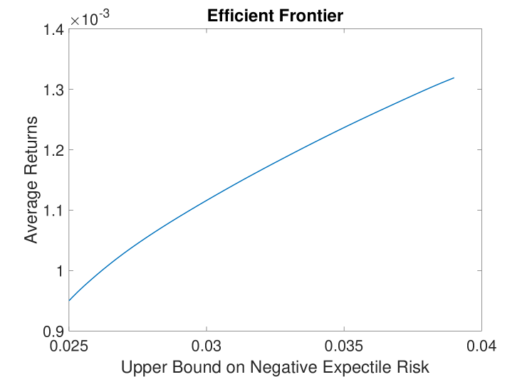
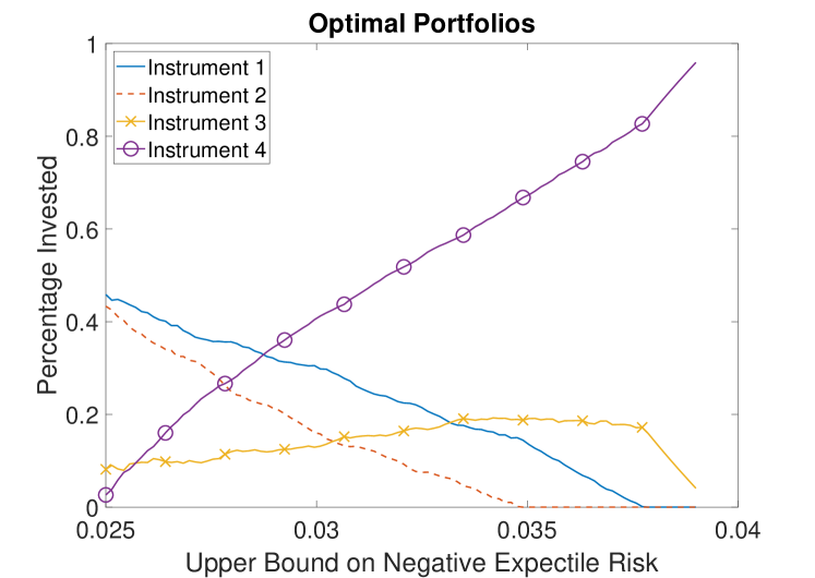
Figure 1. The expected returns of the optimal solution for a range of values of $b$, and the evolution of the optimal portfolio as the constraint on negative expectile risk is loosened.

Figure 1 shows that when the upper bound on negative expectile risk is small, the optimal portfolio is a roughly even mixture of $\xi_{1}$ and $\xi_{2}$. However, as the constraint is loosened, the portfolio gradually shifts to being concentrated in $\xi_{4}$. This indicates that $\xi_{4}$ has the highest expected returns, while also carrying the most risk.

We also consider the problem of minimizing risk with expected returns bounded from below.

$$\min\rho_{q}(x)\quad\text{ s.t}\quad E[\xi^{\intercal}x]\geq r,\ x\geq 0,\ 1^{\intercal}x=1\;.$$

The efficient frontier in Figure 2 shows that until we require an average return of more than $9\times 10^{-4}$, the negative expectile risk of the optimal portfolio is constant. This suggests that in practice a lower bound greater than $9\times 10^{-4}$ may be reasonable. Figure 2 shows that when the constraint on average return is small, the optimal portfolio is an even mix of $\xi_{1}$ and $\xi_{2}$. However, as the constraint on average return increases, the portfolio shifts to the riskier $\xi_{4}$.

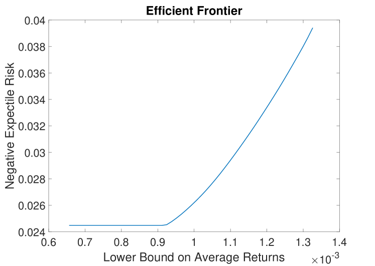
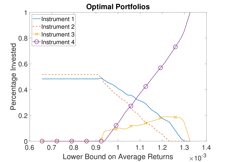
Figure 2. The negative expectile risk of the optimal solution for a range of values of $r$, and the evolution of the optimal portfolio as the constraint on average returns increases.

Lastly, we compare our results with those from the case study “Basic CVaR Optimization Problem, Beyond Black-Litterman” [CVaR Case StudyCVaR Case Study] which uses the same data.

$$\min\text{CVaR}_{0.95}(-\xi^{T}x)\quad\text{ s.t.}\quad E[\xi^{\intercal}x]\geq 0.00105,\ x\geq 0,\ 1^{\intercal}x=1\;.$$

The optimal solution is given by $x=(0.3669,0.2574,0.1304,0.2454)$, which has an average return of $0.00105$ and $\text{CVaR}_{0.95}(-\xi^{T}x)=0.054853$. The optimal solution with the same expected return constraint but minimizing negative expectile is given by $(x=0.357588,0.278139,0.103928,0.260346)$, which has an average return of $0.00105$ and $\rho_{q}(x)=0.027668$.

We also conducted experiments using data from the case study “Omega Portfolio Rebalancing” [Omega Case StudyOmega Case Study]. The first experiment is a numerical test of Corollary 8. We set $z=19$ such that $q=(1+z)^{-1}=0.05$ and solved $(P2,\rho_{(1+z)^{-1}},r)$ for values of $r$ between $10^{-5}$ and $3\times 10^{-4}$. For each $r$ and its corresponding optimal portfolio $x_{0}$, we then solved $(P2,\phi_{-\rho_{(1+z)^{-1}}(x_{0})},r)$ and obtained an optimal portfolio $x_{1}$. According to Corollary 8, if $z>1$, an optimal solution $x_{0}$ of $(P2,\rho_{(1+z)^{-1}},r)$ is also optimal for $(P2,\phi_{-\rho_{(1+z)^{-1}}(x_{0})},r)$ as long as $\xi^{T}x_{0}$ is non-constant. Indeed, this result is supported by the experiment because for each $r$, the portfolios $x_{0}$ and $x_{1}$ were essentially equal. The largest difference in the percentage invested in any instrument between $x_{0}$ and $x_{1}$ was $0.017\%$ over all $r$ tested. We repeated the experiment with the dataset with $10,000$ scenarios from the previous case study and obtained similar results. We remark that the linear programming formulation of omega maximization due to mausser2006optimising took approximately $10$ seconds with this larger dataset while omega maximization with the convex programming approach afforded by PSG took approximately $0.5$ seconds.

We also used this data to compare negative expectile to CVaR and VaR. For a range of values of $r$ between $10^{-5}$ and $3\times 10^{-4}$, we solved the following optimization problems for $q=0.05$ and $\alpha=0.95$.

$$\min\rho_{q}(\xi^{T}x),\ CVaR_{\alpha}(-\xi^{T}x),\ \text{or }VaR_{\alpha}(-\xi^{T}x)\quad\text{ s.t}\quad E[\xi^{\intercal}x]\geq r,\ x\geq 0,\ 1^{\intercal}x=1.$$

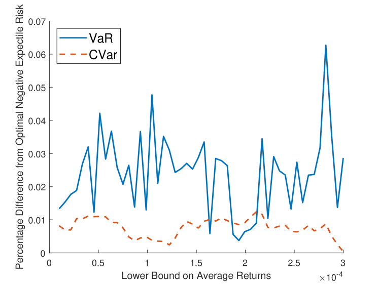
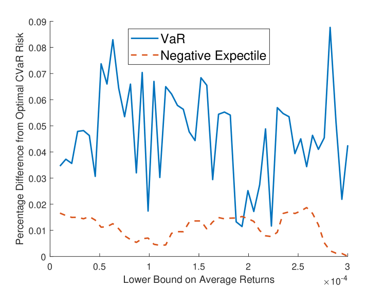
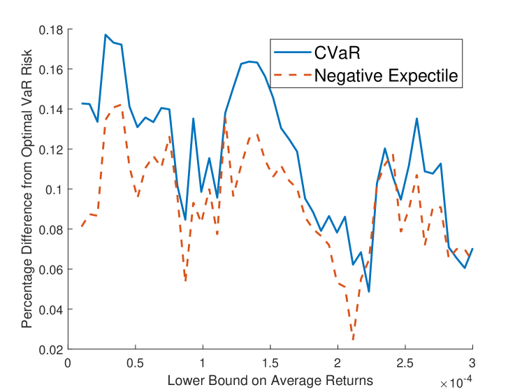
Figure 3. The relative difference between negative expectile, CVaR, and VaR of optimal portfolios.

For each $r$, we obtained an optimal solution for each risk measure and computed the value of this solution with respect to the other two risk measures. Figure 3 plots the relative differences. For example, the first plot shows the negative expectile risk of the optimal VaR and CVaR portfolios for a range of values of $r$. The plots show that the CVaR of the optimal expectile solution and the negative expectile of the optimal CVaR solution are both nearly optimal while the VaRs of the optimal CVaR and expectile solutions are considerably larger. Hence, this experiment suggests that CVaR and negative expectile may be more similar to each other than either is to VaR.

7. Conclusion

This paper considered the optimization problems of maximizing a portfolio’s expected returns with an upper bound constraint on negative expectile risk or minimizing a portfolio’s negative expectile risk with a lower bound constraint on expected returns. We proved equivalences between both of these problems and omega ratio optimization problems in Section 3 by using the inverse relationship between expectile and the omega ratio described in Proposition 2. In order to solve expectile portfolio optimization problems using convex programming in Section 6, we derived a subgradient for $\rho_{q}(x)$, the negative level-$q$ expectile risk of a portfolio $x$. This was done in Section 4 by applying the theory of rockafellar2006optimality to the dual representation of negative expectile due to bellini2014generalized and again in Section 5 by an elementary argument. In Section 6, we also conducted a numerical test of an equivalence between expectile and omega ratio optimization and performed a comparison of negative expectile to two other popular risk measures, VaR and CVaR.

References

- [\citeauthoryearArtzner, Delbaen, Eber, and HeathArtzner et al.1999] Artzner, P., F. Delbaen, J.-M. Eber, and D. Heath (1999). Coherent measures of risk. Mathematical Finance 9(3), 203–228.
- [\citeauthoryearBellini and BernardinoBellini and Bernardino2017] Bellini, F. and E. D. Bernardino (2017). Risk management with expectiles. The European Journal of Finance 23(6), 487–506.
- [\citeauthoryearBellini, Bignozzi, and PuccettiBellini et al.2018] Bellini, F., V. Bignozzi, and G. Puccetti (2018). Conditional expectiles, time consistency and mixture convexity properties. Insurance: Mathematics and Economics 82, 117 – 123.
- [\citeauthoryearBellini, Klar, and MüllerBellini et al.2018] Bellini, F., B. Klar, and A. Müller (2018). Expectiles, omega ratios and stochastic ordering. Methodology and Computing in Applied Probability 20(3), 855–873.
- [\citeauthoryearBellini, Klar, Müller, and GianinBellini et al.2014] Bellini, F., B. Klar, A. Müller, and E. R. Gianin (2014). Generalized quantiles as risk measures. Insurance: Mathematics and Economics 54, 41 – 48.
- [\citeauthoryearBellini, Negri, and PyatkovaBellini et al.2019] Bellini, F., I. Negri, and M. Pyatkova (2019). Backtesting VaR and expectiles with realized scores. Statistical Methods & Applications 28(1), 119–142.
- [\citeauthoryearCVaR Case StudyCVaR Case Study] CVaR Case Study. Case study: Basic CVaR optimization problem, beyond Black-Litterman. https://www.ise.ufl.edu/uryasev/research/testproblems/financial_engineering/basic-cvar-optimization-problem-beyond-black-litterman/. Accessed:2019-6-28.
- [\citeauthoryearExpectiles Case StudyExpectiles Case Study] Expectiles Case Study. Case study: Portfolio optimization with expectiles. https://www.ise.ufl.edu/uryasev/research/testproblems/financial_engineering/case-study-portfolio-optimization-with-expectiles/. Accessed:2019-6-28.
- [\citeauthoryearJakobsonsJakobsons2016] Jakobsons, E. (2016). Scenario aggregation method for portfolio expectile optimization. Statistics & Risk Modeling 33.
- [\citeauthoryearKane, Bartholomew-Biggs, Cross, and DewarKane et al.2009] Kane, S. J., M. C. Bartholomew-Biggs, M. Cross, and M. Dewar (2009). Optimizing omega. Journal of Global Optimization 45(1), 153–167.
- [\citeauthoryearKapsos, Zymler, Christofides, and RustemKapsos et al.2014] Kapsos, M., S. Zymler, N. Christofides, and B. Rustem (2014). Optimizing the omega ratio using linear programming. The Journal of Computational Finance 17(4), 49–57.
- [\citeauthoryearKeating and ShadwickKeating and Shadwick2002] Keating, C. and W. Shadwick (2002). A universal performance measure. Journal of Performance Measurement 6.
- [\citeauthoryearMausser, Saunders, and SecoMausser et al.2006] Mausser, H., D. Saunders, and L. Seco (2006). Optimising omega. Risk 19(11), 88.
- [\citeauthoryearNewey and PowellNewey and Powell1987] Newey, W. K. and J. L. Powell (1987). Asymmetric least squares estimation and testing. Econometrica 55(4), 819–847.
- [\citeauthoryearOmega Case StudyOmega Case Study] Omega Case Study. Case study: Omega portfolio rebalancing. https://www.ise.ufl.edu/uryasev/research/testproblems/financial_engineering/omega-portfolio-rebalancing/. Accessed:2019-6-28.
- [\citeauthoryearRockafellar, Uryasev, and ZabarankinRockafellar et al.2006a] Rockafellar, R. T., S. Uryasev, and M. Zabarankin (2006a). Generalized deviations in risk analysis. Finance and Stochastics 10(1), 51–74.
- [\citeauthoryearRockafellar, Uryasev, and ZabarankinRockafellar et al.2006b] Rockafellar, R. T., S. Uryasev, and M. Zabarankin (2006b). Optimality conditions in portfolio analysis with general deviation measures. Mathematical Programming 108(2), 515–540.
- [\citeauthoryearZiegelZiegel2016] Ziegel, J. F. (2016). Coherence and elicitability. Mathematical Finance 26(4), 901–918.