Constrained polynomial likelihoodthanks: We are grateful to Don Andrews, Oleg Bondarenko, Albina Danilova, Marc Van Uffelen, and participants at the 2021 SoFiE Conference (San Diego), 2021 Brazilian Meeting of Finance, Lunchtime Workshop at Boston University, and the Remote Seminar Series on Computational Economics and Finance for helpful comments. Paul Schneider gratefully acknowledges the SNF grant 100018_189086 “Scenarios”.

Caio Almeida   Ricardo Masini   Paul Schneider calmeida@princeton.edu, Department of Economics and BCF, Princeton University, Princeton, NJ 08544, USA.rmasini@ucdavis.edu, UC Davis, Davis, CA 95616, USA.paul.schneider@usi.ch, USI Lugano and SFI, Lugano, 6900, Switzerland.
Abstract

We develop a non-negative polynomial minimum-norm likelihood ratio (PLR) of two distributions of which only moments are known. The sample PLR converges to the unknown population PLR under mild conditions. The methodology allows for additional shape restrictions, as we illustrate with two empirical applications. The first develops a PLR for the unknown transition density of a jump-diffusion process, while the second extracts a positive density directly from option prices. In both cases, we show the importance of implementing the non-negativity restriction.

Keywords: Likelihood ratio, positive polynomial

1 Introduction

In Hilbert spaces, orthogonality and minimum-norm problems are tightly related. As a consequence, orthogonal polynomials have a prominent role in minimum-norm approximation of unknown likelihood ratios and numeric integration. However, extant approaches based on orthogonality only do not preserve important properties of the approximated objects. In this paper, we develop projections of likelihood ratios onto positive polynomials, thus preserving positivity, and if desired, additional structural constraints.

The literature considers approximations of likelihood ratios with orthogonal polynomials foremost due to the link between polynomials and the possibility of expressing moments of a distribution as expectations of polynomials (Aït-Sahalia, 2002; Filipović et al., 2013; Kato and Kuriki, 2013; Renner and Schmedders, 2015). While many other approaches exist in the literature to approximate likelihood ratios,111The literature on density approximations ranges from saddlepoint approximations (Aït-Sahalia and Yu, 2006), small time expansions (Yu, 2007), to simulation-based methods (Mijatović and Schneider, 2010; Giesecke and Schwenkler, 2018) to cite a small subset of the econometrics and statistics literature. In machine learning, starting from Berlinet and Thomas-Agnan (2004) a sequence of papers embeds distributions in Reproducing Kernel Hilbert Spaces (Song et al., 2009; Grünewälder et al., 2012; Park and Muandet, 2020; Klebanov et al., 2020), as well as likelihood ratios (Schuster et al., 2020). While some of the aforementioned papers preserve positivity and normalization of distributions, they do not provide the flexibility to include additional shape constraints. polynomials are a natural choice, as moments are known for many models such as the large affine class (Duffie et al., 2003). Moreover, under mild technical conditions, polynomials generate weighted L2superscript𝐿2L^{2} spaces that arise naturally when working with expectations and sample averages. In our paper, we work with positive polynomials with the smallest modification to the extant expansions mentioned above.222More generally, we operate within the generic Hilbert space problem  minimize gg, subject to (g,f)C,fformulae-sequence𝑔 minimize norm𝑔 subject to 𝑔𝑓𝐶𝑓\displaystyle\underset{g\in\mathcal{H}}{\text{ minimize }}\left\|g\right\|,\text{ subject to }(g,f)\in C,\,f\in\mathcal{H} where C𝐶C is a convex set, and \mathcal{H} is a Hilbert space along with its inner product (,)(\cdot,\cdot), encompassing function approximation, interpolation, and many other applications. In this paper, we specialize in likelihood ratios with probabilistic models in mind.

Our framework, rooted in Grenander (1981) sieve estimation, is built upon several steps. First, we consider the conventional projection of a likelihood ratio on polynomials. Through an optimization problem, we then obtain our polynomial minimum-norm likelihood ratio (PLR) as the sum of this element, and the minimum-norm polynomial that guarantees pointwise positivity. We show that this optimization problem, if feasible, has the PLR as its unique solution, and subsequently prove consistency of the PLR based on sample moments. Importantly, these coefficients of the PLR can be obtained rapidly as the solution of a conic optimization program, allowing also for additional constraints that can modify the shape of the PLR.

The sieves literature nonparametrically approximates a function using a sequence of finite-dimensional spaces and corresponding basis functions, such as polynomials, splines, wavelets, and trigonometric functions, that grow with the sample size to asymptotically eliminate the bias in the estimation process (see Chen (2007)). In contrast, we opt to keep the degree of the PLR polynomial fixed, approximating the pseudo-true likelihood with (potential) bias. Our motivation stems from the fact that preserving positivity is more important when a finite sample size caps the maximum degree of the PLR than in a limiting large sample/large polynomial degree environment, where the estimated PLR would converge to its positive population counterpart.

A related literature beginning with Hansen and Scheinkman (2009) emphasizes the importance of positive eigenfunctions in asset pricing problems333Hansen and Scheinkman (2009) propose an operator approach to study the long-run risk-return trade-off properties of Stochastic Discount Factors (SDFs) in Markovian environments by solving a Perron-Frobenious eigenfunction problem. The SDF is decomposed into a permanent (martingale) and a transitory component (see Alvarez and Jermann (2005)). Ross (2015) uses the Perron-Frobenious approach to recover investors’ beliefs, i.e., subjective probabilities under rational expectations. Borovička et al. (2016) discuss the conditions under which the probability recovered with Perron-Frobenious coincides with the actual probabilities of investors under rational expectations. Christensen (2017) proposes using Sieves to empirically identify this SDF decomposition, establishing the asymptotic theory for Perron-Frobenious eigenfunction and eigenvalue estimators. A non-exhaustive list of additional papers on the SDF decomposition and on recovery probabilities include Chabi-Yo and Bakshi (2012), Chabi-Yo et al. (2015), Backus et al. (2014), Qin and Linetsky (2016), and Qin and Linetsky (2017).. Preserving positivity is fundamental in such problems, for instance, in Christensen (2017), who provide Hermite polynomial approximations for estimating a nonparametric decomposition of the Stochastic Discount Factor in transitory and permanent components. In this context, our methodology could be used to guarantee a non-negative approximation to the positive eigenfunctions that define the SDF decomposition in finite samples where a projection on polynomials is not guaranteed to preserve positivity.

We illustrate the usefulness of PLR with two simple applications. In the first, we expand the likelihood ratio of the transition density of a continuous-time jump-diffusion process with respect to a Gamma density.444When expanding a transition density it is necessary to choose an appropriate auxiliary density function on the same support. For positive support, the Gamma distribution is suited (see Filipović et al. (2013)). While the conventional orthogonal polynomial approach produces an approximation that is negative close to zero, our PLR is non-negative everywhere and thus can be readily used in any context that crucially relies on the structural properties, normalization, and positivity, of probability measures, such as accept-reject sampling or Bayesian modeling.

In our second application, we subsequently investigate how to extract probability densities directly from option prices. This is particularly interesting in the context of pricing exotic and/or over-the-counter derivatives based on the probability density extracted from vanilla observed option prices. We illustrate this procedure in a controlled environment with a bivariate continuous-time jump-diffusion process from Duffie et al. (2000). Our experiments reveal how the positivity of the PLR crucially translates into meaningful estimates of positive probability densities, rather than projections of densities that do not share basic defining properties of probability measures.

The paper is organized as follows. In Section 2.1 we develop the necessary notation. The traditional approach to minimum-norm expansions appears in Section 2.2 for reference. In Section 2.3 we propose modifications to the standard program to ensure positivity. Section 2.4 shows the uniqueness, consistency, and rate of convergence of the polynomial coefficients defining the PLR. Applications are presented in Sections 3.1 (density approximations), and 3.2 (option pricing). Section 4 concludes. In the Appendix, we review sum-of-squares (s.o.s.) polynomials and include the proofs for the theoretical results.

2 Constrained polynomial likelihood

2.1 Set-up and notation

Denoting by 𝒫𝒫\mathcal{P} a probability measure on Dd𝐷superscript𝑑D\subseteq\mathbb{R}^{d}, let L𝒫2superscriptsubscript𝐿𝒫2L_{\mathcal{P}}^{2} be the equivalence class of functions f:D:𝑓maps-to𝐷f:D\mapsto\mathbb{\mathbb{R}} such that Df2(t)𝑑𝒫(t)<subscript𝐷superscript𝑓2𝑡differential-d𝒫𝑡\int_{D}f^{2}(t)d\mathcal{P}(t)<\infty with inner product

(f,g)=Df(t)g(t)𝑑𝒫(t),f,gL𝒫2,t:=[t1,,td],formulae-sequence𝑓𝑔subscript𝐷𝑓𝑡𝑔𝑡differential-d𝒫𝑡𝑓formulae-sequence𝑔subscriptsuperscript𝐿2𝒫assign𝑡subscript𝑡1subscript𝑡𝑑\begin{split}(f,g)=\int_{D}{f(t)g(t)d\mathcal{P}(t)},\,f,g\in L^{2}_{\mathcal{P}},\,t:=[t_{1},\ldots,t_{d}],\end{split} (1)

where we allow in subsequent sections to extend the inner product to act element-wise on matrices.

Denote by [t]delimited-[]𝑡\mathbb{R}[t] the ring of square-integrable polynomials on dsuperscript𝑑\mathbb{R}^{d}, and by [t]nsubscriptdelimited-[]𝑡𝑛\mathbb{R}[t]_{n} the subset of polynomials ξ[t]𝜉delimited-[]𝑡\xi\in\mathbb{R}[t] with deg(ξ)ndegree𝜉𝑛\deg(\xi)\leq n. Denote further by P𝒫,nsubscript𝑃𝒫𝑛P_{\mathcal{P},n} the set of polynomials [t]nsubscriptdelimited-[]𝑡𝑛\mathbb{R}[t]_{n} endowed with inner product (1), a finite-dimensional Hilbert space.

From the standard canonical monomial basis of P𝒫,nsubscript𝑃𝒫𝑛P_{\mathcal{P},n} we denote

𝝉n(t):=[1,t1,,td,t12,t1t2,,td2,,t1n,t1n1t2,,tdn],assignsubscript𝝉𝑛𝑡superscript1subscript𝑡1subscript𝑡𝑑superscriptsubscript𝑡12subscript𝑡1subscript𝑡2superscriptsubscript𝑡𝑑2superscriptsubscript𝑡1𝑛superscriptsubscript𝑡1𝑛1subscript𝑡2superscriptsubscript𝑡𝑑𝑛top\bm{\tau}_{n}(t):=[1,t_{1},\ldots,t_{d},t_{1}^{2},t_{1}t_{2},\ldots,t_{d}^{2},\ldots,t_{1}^{n},t_{1}^{n-1}t_{2},\ldots,t_{d}^{n}]^{\top}, (2)

as well as multi-index powers t𝜷:=t1β1tdβdassignsuperscript𝑡𝜷superscriptsubscript𝑡1subscript𝛽1superscriptsubscript𝑡𝑑subscript𝛽𝑑t^{\bm{\beta}}:=t_{1}^{\beta_{1}}\cdots t_{d}^{\beta_{d}} for 𝜷0d𝜷subscriptsuperscript𝑑0\bm{\beta}\in\mathbb{N}^{d}_{0}, where the length of the multi-index is |𝜷|=β1++βd𝜷subscript𝛽1subscript𝛽𝑑\lvert\bm{\beta}\rvert=\beta_{1}+\cdots+\beta_{d} .

There are (n+dd)binomial𝑛𝑑𝑑\binom{n+d}{d} elements in the monomial basis, and we denote by α0,,αNsubscript𝛼0subscript𝛼𝑁\alpha_{0},\ldots,\alpha_{N}, with N=(n+dd)1𝑁binomial𝑛𝑑𝑑1N=\binom{n+d}{d}-1, the multi-indices corresponding to their order of appearance in (2). For example, the second element is t𝜶1=t1α11tdα1d=t11t20td0=t1superscript𝑡subscript𝜶1superscriptsubscript𝑡1subscript𝛼11superscriptsubscript𝑡𝑑subscript𝛼1𝑑superscriptsubscript𝑡11superscriptsubscript𝑡20superscriptsubscript𝑡𝑑0subscript𝑡1t^{\bm{\alpha}_{1}}=t_{1}^{\alpha_{11}}\cdots t_{d}^{\alpha_{1d}}=t_{1}^{1}t_{2}^{0}\cdots t_{d}^{0}=t_{1}. Any polynomial ξnP𝒫,nsubscript𝜉𝑛subscript𝑃𝒫𝑛\xi_{n}\in P_{\mathcal{P},n} can be written as ξn=𝒙𝝉nsubscript𝜉𝑛superscript𝒙topsubscript𝝉𝑛\xi_{n}=\bm{x}^{\top}\bm{\tau}_{n}, where 𝒙N+1𝒙superscript𝑁1\bm{x}\in\mathbb{R}^{N+1} is a coefficient vector.

With projections on positive polynomials in mind, we parameterize a particularly tractable cone Mn(D)P𝒫,nsubscript𝑀𝑛𝐷subscript𝑃𝒫𝑛M_{n}(D)\subset P_{\mathcal{P},n} of positive polynomials as follows.

Definition 2.1 (Positive s.o.s. polynomials).

Let S+q,qsuperscriptsubscript𝑆𝑞𝑞S_{+}^{q},q\in\mathbb{N} denote the set of symmetric positive semidefinite (p.s.d.) matrices of dimension q𝑞q. We denote by Mn(D)subscript𝑀𝑛𝐷M_{n}(D) the set of positive polynomials ξn(t)=𝒙𝝉n(t)0,tDformulae-sequencesubscript𝜉𝑛𝑡superscript𝒙topsubscript𝝉𝑛𝑡0for-all𝑡𝐷\xi_{n}(t)=\bm{x}^{\top}\bm{\tau}_{n}(t)\geq 0,\forall t\in D for matrices 𝑽S+qV𝑽superscriptsubscript𝑆subscript𝑞𝑉\bm{V}\in S_{+}^{q_{V}} and 𝑾S+qW𝑾superscriptsubscript𝑆subscript𝑞𝑊\bm{W}\in S_{+}^{q_{W}} on a case-by-case basis.

  1. 1.

    Case D=d𝐷superscript𝑑D=\mathbb{R}^{d}: ξn(t)=𝝉n/2(t)𝑽𝝉n/2(t),subscript𝜉𝑛𝑡superscriptsubscript𝝉𝑛2top𝑡𝑽subscript𝝉𝑛2𝑡\xi_{n}(t)=\bm{\tau}_{n/2}^{\top}(t)\,\bm{V}\,\bm{\tau}_{n/2}(t),

  2. 2.

    Case D=+𝐷subscriptD=\mathbb{R}_{+}: ξn(t)=𝝉n/2(t)𝑽𝝉n/2(t)+t(𝝉n/21(t)𝑾𝝉n/21(t)),subscript𝜉𝑛𝑡superscriptsubscript𝝉𝑛2top𝑡𝑽subscript𝝉𝑛2𝑡𝑡superscriptsubscript𝝉𝑛21top𝑡𝑾subscript𝝉𝑛21𝑡\xi_{n}(t)=\bm{\tau}_{n/2}^{\top}(t)\,\bm{V}\,\bm{\tau}_{n/2}(t)+t\left(\bm{\tau}_{n/2-1}^{\top}(t)\,\bm{W}\,\bm{\tau}_{n/2-1}(t)\right),,

  3. 3.

    Case D=[a,b]𝐷𝑎𝑏D=[a,b]: ξn(t)=𝝉n/2(t)𝑽𝝉n/2(t)+(bt)(ta)(𝝉n/21(t)𝑾𝝉n/21(t)).subscript𝜉𝑛𝑡superscriptsubscript𝝉𝑛2top𝑡𝑽subscript𝝉𝑛2𝑡𝑏𝑡𝑡𝑎superscriptsubscript𝝉𝑛21top𝑡𝑾subscript𝝉𝑛21𝑡\xi_{n}(t)=\bm{\tau}_{n/2}^{\top}(t)\,\bm{V}\,\bm{\tau}_{n/2}(t)+(b-t)(t-a)\left(\bm{\tau}_{n/2-1}^{\top}(t)\,\bm{W}\,\bm{\tau}_{n/2-1}(t)\right).

By collecting coefficients in the relation above, we can identify a linear relation 𝒙=T(𝑽,𝑾)𝒙𝑇𝑽𝑾\bm{x}=T(\bm{V},\bm{W}) between the coefficient vector 𝒙𝒙\bm{x} of a positive polynomial in Mn(D)subscript𝑀𝑛𝐷M_{n}(D) to elements of the symmetric positive semidefinite (p.s.d.) matrices 𝑽𝑽\bm{V} and 𝑾𝑾\bm{W}, whose dimensions are qV=(n/2+dd)subscript𝑞𝑉binomial𝑛2𝑑𝑑q_{V}=\binom{n/2+d}{d} and qW=0subscript𝑞𝑊0q_{W}=0 in the first case, and qV=(n/2+11)subscript𝑞𝑉binomial𝑛211q_{V}=\binom{n/2+1}{1} and qW=(n/21)subscript𝑞𝑊binomial𝑛21q_{W}=\binom{n/2}{1} in the latter two cases. As outlined in Appendix A, Definition 2.1 characterizes the set of positive polynomials in the univariate case, but it is only sufficient in the multivariate case, for which positive polynomials exist that are not sums of squares. As the benefit of the above s.o.s. parameterization, positive polynomials can be modellied through semidefinite programming. Without further modifications, the linear transformation T𝑇T is not a bijection in general, however, as the following example shows.

Example 1 (Selection matrices).

Suppose that n=4𝑛4n=4, and D=𝐷D=\mathbb{R}. Then positivity requires

𝝉4(t)𝒙=𝝉2(t)𝑽𝝉2(t)=tr(𝑽𝝉2(t)𝝉2(t))=tr([V11V21V31V21V22V32V31V32V33][1tt2tt2t3t2t3t4]).superscriptsubscript𝝉4top𝑡𝒙superscriptsubscript𝝉2top𝑡𝑽subscript𝝉2𝑡tr𝑽subscript𝝉2𝑡superscriptsubscript𝝉2top𝑡trmatrixsubscript𝑉11subscript𝑉21subscript𝑉31subscript𝑉21subscript𝑉22subscript𝑉32subscript𝑉31subscript𝑉32subscript𝑉33matrix1𝑡superscript𝑡2𝑡superscript𝑡2superscript𝑡3superscript𝑡2superscript𝑡3superscript𝑡4\bm{\tau}_{4}^{\top}(t)\bm{x}=\bm{\tau}_{2}^{\top}(t)\,\bm{V}\,\bm{\tau}_{2}(t)=\operatorname{tr}\left(\bm{V}\bm{\tau}_{2}(t)\bm{\tau}_{2}^{\top}(t)\right)=\operatorname{tr}\left(\begin{bmatrix}V_{11}&V_{21}&V_{31}\\ V_{21}&V_{22}&V_{32}\\ V_{31}&V_{32}&V_{33}\end{bmatrix}\begin{bmatrix}1&t&t^{2}\\ t&t^{2}&t^{3}\\ t^{2}&t^{3}&t^{4}\end{bmatrix}\right).

Collecting coefficients, we can thus express the selection matrices as

𝑽0=[100000000],𝑽1=[010100000],𝑽2=[001010100],𝑽3=[000001010],𝑽4=[000000001],formulae-sequencesubscript𝑽0matrix100000000formulae-sequencesubscript𝑽1matrix010100000formulae-sequencesubscript𝑽2matrix001010100formulae-sequencesubscript𝑽3matrix000001010subscript𝑽4matrix000000001\bm{V}_{0}=\begin{bmatrix}1&0&0\\ 0&0&0\\ 0&0&0\end{bmatrix},\bm{V}_{1}=\begin{bmatrix}0&1&0\\ 1&0&0\\ 0&0&0\end{bmatrix},\bm{V}_{2}=\begin{bmatrix}0&0&1\\ 0&1&0\\ 1&0&0\end{bmatrix},\bm{V}_{3}=\begin{bmatrix}0&0&0\\ 0&0&1\\ 0&1&0\end{bmatrix},\bm{V}_{4}=\begin{bmatrix}0&0&0\\ 0&0&0\\ 0&0&1\end{bmatrix},

such that [x0,x1,x2,x3,x4]=T(𝑽)=[tr(𝑽𝑽i)]i=04=[V11,2V21,V22+2V31,2V32,V33].subscript𝑥0subscript𝑥1subscript𝑥2subscript𝑥3subscript𝑥4superscript𝑇top𝑽superscriptsubscriptdelimited-[]tr𝑽subscript𝑽𝑖𝑖04subscript𝑉112subscript𝑉21subscript𝑉222subscript𝑉312subscript𝑉32subscript𝑉33[x_{0},x_{1},x_{2},x_{3},x_{4}]=T^{\top}(\bm{V})=[\operatorname{tr}\left(\bm{V}\bm{V}_{i}\right)]_{i=0}^{4}=[V_{11},2V_{21},V_{22}+2V_{31},2V_{32},V_{33}].

Before presenting the full type of problems we are intending to solve on Mn(D)subscript𝑀𝑛𝐷M_{n}(D), we briefly review projections of Radon-Nikodym derivatives on polynomials through equality-constrained minimum-norm problems. While this problem is standard, and its solution is well-known, it helps inform the optimization program for the shape-constrained version in the subsequent section.

2.2 Minimum-norm likelihood ratio projection

For projections in L2subscriptsuperscript𝐿2L^{2}_{\mathbb{P}}, with or without shape constraints, the Gram matrix

𝑯n:=(𝝉n,𝝉n)=[μ0,0𝒫μ0,1𝒫μ0,N𝒫μ1,0𝒫μ1,1𝒫μ1,N𝒫μN,0𝒫μN,1𝒫μN,N𝒫], with μi,j𝒫:=Dtαi+αj𝑑𝒫(t)formulae-sequenceassignsubscript𝑯𝑛subscript𝝉𝑛superscriptsubscript𝝉𝑛topmatrixsuperscriptsubscript𝜇00𝒫superscriptsubscript𝜇01𝒫superscriptsubscript𝜇0𝑁𝒫superscriptsubscript𝜇10𝒫superscriptsubscript𝜇11𝒫superscriptsubscript𝜇1𝑁𝒫superscriptsubscript𝜇𝑁0𝒫superscriptsubscript𝜇𝑁1𝒫superscriptsubscript𝜇𝑁𝑁𝒫assign with superscriptsubscript𝜇𝑖𝑗𝒫subscript𝐷superscript𝑡subscript𝛼𝑖subscript𝛼𝑗differential-d𝒫𝑡\bm{H}_{n}:=(\bm{\tau}_{n},\bm{\tau}_{n}^{\top})=\begin{bmatrix}\mu_{0,0}^{\mathcal{P}}&\mu_{0,1}^{\mathcal{P}}&\cdots&\mu_{0,N}^{\mathcal{P}}\\ \mu_{1,0}^{\mathcal{P}}&\mu_{1,1}^{\mathcal{P}}&\cdots&\mu_{1,N}^{\mathcal{P}}\\ \vdots&\vdots&\ddots&\vdots\\ \mu_{N,0}^{\mathcal{P}}&\mu_{N,1}^{\mathcal{P}}&\cdots&\mu_{N,N}^{\mathcal{P}}\end{bmatrix},\text{ with }\mu_{i,j}^{\mathcal{P}}:=\int_{D}t^{\alpha_{i}+\alpha_{j}}d\mathcal{P}(t) (3)

features prominently. Our first assumption regarding this symmetric and positive semidefinite matrix greatly simplifies further analysis. It is mild, easily checked, and ensures in particular that the inverse of the Gram matrix 𝑯1superscript𝑯1\bm{H}^{-1} is readily available, greatly facilitating the analysis below.

Assumption 2.2 (Rank of 𝑯nsubscript𝑯𝑛\bm{H}_{n}).

Gram matrix 𝑯nsubscript𝑯𝑛\bm{H}_{n}’s smallest eigenvalue λmin(𝑯n)>0subscript𝜆subscript𝑯𝑛0\lambda_{\min}(\bm{H}_{n})>0.

We are particularly interested in projections on polynomials of the Radon-Nikodym derivative of a probability measure 𝒬𝒬\mathcal{Q} on D𝐷D that is absolutely continuous with respect to 𝒫𝒫\mathcal{P}. Finding the minimum-norm such projection on polynomials, where 𝒬𝒬\mathcal{Q} is only known from its moment vector 𝝁𝒬:=[μ0𝒬,,μN𝒬]assignsubscript𝝁𝒬superscriptsuperscriptsubscript𝜇0𝒬superscriptsubscript𝜇𝑁𝒬top\bm{\mu}_{\mathcal{Q}}:=[\mu_{0}^{\mathcal{Q}},\ldots,\mu_{N}^{\mathcal{Q}}]^{\top} with μi𝒬:=Dtαi𝑑𝒬(t)assignsuperscriptsubscript𝜇𝑖𝒬subscript𝐷superscript𝑡subscript𝛼𝑖differential-d𝒬𝑡\mu_{i}^{\mathcal{Q}}:=\int_{D}t^{\alpha_{i}}d\mathcal{Q}(t), solves the equivalent problems (Luenberger, 1997)

minimize ξnP𝒫,nd𝒬d𝒫ξn2subscript𝜉𝑛subscript𝑃𝒫𝑛minimize superscriptnorm𝑑𝒬𝑑𝒫subscript𝜉𝑛2\underset{\xi_{n}\in P_{\mathcal{P},n}}{\text{minimize }}\left\|\frac{d\mathcal{Q}}{d\mathcal{P}}-\xi_{n}\right\|^{2}

\Leftrightarrow minimize 𝒙N𝑯n1/2𝒙22,subject to 𝑯n𝒙=𝝁𝒬,𝒙superscript𝑁minimize superscriptsubscriptdelimited-∥∥superscriptsubscript𝑯𝑛12𝒙22subject to subscript𝑯𝑛𝒙subscript𝝁𝒬\begin{split}\underset{\bm{x}\in\mathbb{R}^{N}}{\text{minimize }}&\left\|\bm{H}_{n}^{1/2}\,\bm{x}\right\|_{2}^{2},\,\text{subject to }\\ \bm{H}_{n}\bm{x}&=\bm{\mu}_{\mathcal{Q}},\\ \end{split} (4) where 𝑯n1/2superscriptsubscript𝑯𝑛12\bm{H}_{n}^{1/2} denotes the Cholesky factor of 𝑯nsubscript𝑯𝑛\bm{H}_{n}. The well-known solution to problem (4) is

ξn(t):=𝝁𝒬𝑯n1𝝉n(t).assignsuperscriptsubscript𝜉𝑛𝑡superscriptsubscript𝝁𝒬topsuperscriptsubscript𝑯𝑛1subscript𝝉𝑛𝑡\xi_{n}^{\star}(t):=\bm{\mu}_{\mathcal{Q}}^{\top}\bm{H}_{n}^{-1}\bm{\tau}_{n}(t). (5)

On P𝒫,nsubscript𝑃𝒫𝑛P_{\mathcal{P},n}, the projection of a Radon-Nikodym derivative on polynomials evidently corresponds to moment-matching. However, there is no mechanism that ensures to maintain the structural properties of Radon-Nikodym derivatives – normalization and positivity – in the projection.

To project on positive polynomials, with Mn(D)subscript𝑀𝑛𝐷M_{n}(D) not being a linear space, using it as a hypothesis space requires additional considerations. In the next section, we, therefore, introduce an optimization program akin to (4), where membership to Mn(D)subscript𝑀𝑛𝐷M_{n}(D) is implemented as a conic constraint. The formulation as an optimization program additionally allows to generalize the equality constraints in Section 2.2 to inequalities, and to add further restrictions, as demanded by each application.

2.3 Constrained minimum-norm likelihood ratio projection

In this section, we introduce a minimization program that accommodates the constraints in (4) as a special case and includes additionally the conic constraint ξnMn(D)subscript𝜉𝑛subscript𝑀𝑛𝐷\xi_{n}\in M_{n}(D) from Definition 2.1.

minimizeξnMn(D)ξn2, subject to (ξn,fi)=ci,i=1,,m, and (ξn,gj)dj,j=1,,l,formulae-sequencesubscript𝜉𝑛subscript𝑀𝑛𝐷minimizesuperscriptdelimited-∥∥subscript𝜉𝑛2 subject to subscript𝜉𝑛subscript𝑓𝑖subscript𝑐𝑖formulae-sequence𝑖1𝑚formulae-sequence and subscript𝜉𝑛subscript𝑔𝑗subscript𝑑𝑗𝑗1𝑙\begin{split}\underset{\xi_{n}\in M_{n}(D)}{\text{minimize}}&\left\|\xi_{n}\right\|^{2},\text{ subject to }\\ (\xi_{n},f_{i})&=c_{i},\,i=1,\ldots,m,\text{ and }(\xi_{n},g_{j})\leq d_{j},\,j=1,\ldots,l,\end{split} (6)

where f1,,fm,g1,,glL𝒫2subscript𝑓1subscript𝑓𝑚subscript𝑔1subscript𝑔𝑙subscriptsuperscript𝐿2𝒫f_{1},\ldots,f_{m},g_{1},\ldots,g_{l}\in L^{2}_{\mathcal{P}} are linearly independent functions generating the subspace K:=[f1,,fm,g1,,gl]assign𝐾subscript𝑓1subscript𝑓𝑚subscript𝑔1subscript𝑔𝑙K:=[f_{1},\ldots,f_{m},g_{1},\ldots,g_{l}]. While in general KP𝒫,n𝐾subscript𝑃𝒫𝑛K\varsubsetneq P_{\mathcal{P},n}, we nevertheless routinely set f1=1subscript𝑓11f_{1}=1, so that with (ξn,f1)=1subscript𝜉𝑛subscript𝑓11(\xi_{n},f_{1})=1, ξnsubscript𝜉𝑛\xi_{n} represents a normalized and positive likelihood ratio with respect to a probability distribution 𝒫𝒫\mathcal{P}. Together with the additional constraints it therefore is a constrained polynomial likelihood ratio (PLR). Note that the constraint ξnMn(D)subscript𝜉𝑛subscript𝑀𝑛𝐷\xi_{n}\in M_{n}(D) ensures pointwise positivity. This is important for evaluating the PLR with any argument while maintaining positivity, as for instance in out-of-sample exercises or simulations.

It is easy to construct an example for which program (6) is infeasible. The constraint (ξn,1)=1subscript𝜉𝑛11(\xi_{n},1)=-1 can not be satisfied by any non-negative polynomial ξnsubscript𝜉𝑛\xi_{n}, with 𝒫𝒫\mathcal{P} being a probability measure. Apart from such cases, the feasibility of (6) becomes more likely, the higher the order of ξnsubscript𝜉𝑛\xi_{n}, increasing the number of coefficients. In light of this observation, denoting by K~={𝒙N+1:{(ξn,fi)=ci}{i=1,,m}, and {(ξn,gj)dj}{j=1,,l}}~𝐾conditional-set𝒙superscript𝑁1subscriptsubscript𝜉𝑛subscript𝑓𝑖subscript𝑐𝑖𝑖1𝑚 and subscriptsubscript𝜉𝑛subscript𝑔𝑗subscript𝑑𝑗𝑗1𝑙\tilde{K}=\{\bm{x}\in\mathbb{R}^{N+1}:\{(\xi_{n},f_{i})=c_{i}\}_{\{i=1,\ldots,m\}},\text{ and }\{(\xi_{n},g_{j})\leq d_{j}\}_{\{j=1,\ldots,l\}}\} the feasible set of program (6), we state our second assertion.

Assumption 2.3 (Feasibility).

There exists n𝑛n\in\mathbb{N} such that K~~𝐾\tilde{K} has non-empty interior.

In the next section, we discuss a generic solution algorithm to the optimization problem (6), and show the consistency of the solution in the case when the inner product (1) is estimated from sample averages.

2.4 Properties of solutions on P𝒫,nsubscript𝑃𝒫𝑛P_{\mathcal{P},n} and Mn(D)subscript𝑀𝑛𝐷M_{n}(D)

The present section discusses the properties of the solution to program (6).

2.4.1 Uniqueness of the primal optimization problem

As a first step, we argue the uniqueness of the solution to program (6), if the constraints are feasible, as a standard result in finite-dimensional convex optimization. To develop a solution, we first exploit that we work in a finite-dimensional Hilbert space of polynomials, which allows us to express the functional inequalities as matrix equations. The (in)equalities in Eq. (6) are linear in ξnsubscript𝜉𝑛\xi_{n}, and defining 𝒄:=[c1,,cm],𝒅:=[d1,,dl],𝒇:=[f1,,fm]formulae-sequenceassign𝒄superscriptsubscript𝑐1subscript𝑐𝑚topformulae-sequenceassign𝒅superscriptsubscript𝑑1subscript𝑑𝑙topassign𝒇superscriptsubscript𝑓1subscript𝑓𝑚top\bm{c}:=[c_{1},\ldots,c_{m}]^{\top},\,\bm{d}:=[d_{1},\ldots,d_{l}]^{\top},\,\bm{f}:=[f_{1},\ldots,f_{m}]^{\top}, and 𝒈:=[g1,,gl]assign𝒈superscriptsubscript𝑔1subscript𝑔𝑙top\bm{g}:=[g_{1},\ldots,g_{l}]^{\top}, we can express them as

(ξn,𝒇)=𝑭n𝒙=𝒄, and (ξn,𝒈)=𝑮n𝒙𝒅.formulae-sequencesubscript𝜉𝑛𝒇subscript𝑭𝑛𝒙𝒄 and subscript𝜉𝑛𝒈subscript𝑮𝑛𝒙precedes-or-equals𝒅(\xi_{n},\bm{f})=\bm{F}_{n}\bm{x}=\bm{c},\text{ and }(\xi_{n},\bm{g})=\bm{G}_{n}\bm{x}\preceq\bm{d}. (7)

where precedes-or-equals\preceq represents generalized, conic, inequality, and the inner product is naturally applied element-wise, such that 𝑭nm×N+1subscript𝑭𝑛superscript𝑚𝑁1\bm{F}_{n}\in\mathbb{R}^{m\times N+1} and 𝑮nl×N+1subscript𝑮𝑛superscript𝑙𝑁1\bm{G}_{n}\in\mathbb{R}^{l\times N+1}.

Proposition 2.4.

If Assumptions 2.2 and 2.3 hold, problem (6) has a unique solution from the primal problem

minimize 𝒙N+112𝑯n1/2𝒙22,subject to 𝑭n𝒙=𝒄,𝑮n𝒙𝒅,𝒙=T(𝑽,𝑾);𝑽S+mV,𝑾S+mW,formulae-sequence𝒙superscript𝑁1minimize 12superscriptsubscriptdelimited-∥∥superscriptsubscript𝑯𝑛12𝒙22subject to subscript𝑭𝑛𝒙𝒄formulae-sequenceprecedes-or-equalssubscript𝑮𝑛𝒙𝒅formulae-sequence𝒙𝑇𝑽𝑾formulae-sequence𝑽superscriptsubscript𝑆subscript𝑚𝑉𝑾superscriptsubscript𝑆subscript𝑚𝑊\begin{split}\underset{\bm{x}\in\mathbb{R}^{N+1}}{\text{minimize }}&\quad\frac{1}{2}\left\|\bm{H}_{n}^{1/2}\bm{x}\right\|_{2}^{2},\\ \text{subject to }&\bm{F}_{n}\bm{x}=\bm{c},\,\bm{G}_{n}\bm{x}\preceq\bm{d},\\ \bm{x}&=T(\bm{V},\bm{W});\bm{V}\in S_{+}^{m_{V}},\bm{W}\in S_{+}^{m_{W}},\end{split} (8)

where the linear map T:S+mV×S+mWN+1:𝑇maps-tosuperscriptsubscript𝑆subscript𝑚𝑉superscriptsubscript𝑆subscript𝑚𝑊superscript𝑁1T:S_{+}^{m_{V}}\times S_{+}^{m_{W}}\mapsto\mathbb{R}^{N+1},

T(𝑽,𝑾):=[tr(𝑽0𝑽)+tr(𝑾0𝑾),,tr(𝑽N𝑽)+tr(𝑾N𝑾)],assign𝑇𝑽𝑾superscripttrsubscript𝑽0𝑽trsubscript𝑾0𝑾trsubscript𝑽𝑁𝑽trsubscript𝑾𝑁𝑾topT(\bm{V},\bm{W}):=[\operatorname{tr}(\bm{V}_{0}\bm{V})+\operatorname{tr}(\bm{W}_{0}\bm{W}),\cdots,\operatorname{tr}(\bm{V}_{N}\bm{V})+\operatorname{tr}(\bm{W}_{N}\bm{W})]^{\top}, (9)

for fixed symmetric selection matrices 𝐕0,,𝐕Nsubscript𝐕0subscript𝐕𝑁\bm{V}_{0},\ldots,\bm{V}_{N} and 𝐖0,,𝐖Nsubscript𝐖0subscript𝐖𝑁\bm{W}_{0},\ldots,\bm{W}_{N} of the same dimension as 𝐕𝐕\bm{V} and 𝐖𝐖\bm{W}, respectively. The corresponding dual reads

maximize 𝜼m,𝜺+l,𝝂N+112𝑯n1/2(𝑭n𝜼+𝝂𝑮n𝜺)22𝜺𝒅+𝜼𝒄subject to i=0Nνi𝑽i0,i=0Nνi𝑾i0.formulae-sequencesucceeds-or-equalsformulae-sequence𝜼superscript𝑚formulae-sequence𝜺superscriptsubscript𝑙𝝂superscript𝑁1maximize 12superscriptsubscriptdelimited-∥∥subscriptsuperscript𝑯12𝑛superscriptsubscript𝑭𝑛top𝜼𝝂superscriptsubscript𝑮𝑛top𝜺22superscript𝜺top𝒅superscript𝜼top𝒄subject to superscriptsubscript𝑖0𝑁subscript𝜈𝑖subscript𝑽𝑖0succeeds-or-equalssuperscriptsubscript𝑖0𝑁subscript𝜈𝑖subscript𝑾𝑖0\begin{split}\underset{\bm{\eta}\in\mathbb{R}^{m},\bm{\varepsilon}\in\mathbb{R}_{+}^{l},\bm{\nu}\in\mathbb{R}^{N+1}}{\text{maximize }}&-\frac{1}{2}\|\bm{H}^{-1/2}_{n}(\bm{F}_{n}^{\top}\bm{\eta}+\bm{\nu}-\bm{G}_{n}^{\top}\bm{\varepsilon})\|_{2}^{2}-\bm{\varepsilon}^{\top}\bm{d}+\bm{\eta}^{\top}\bm{c}\\ \text{subject to }&\sum_{i=0}^{N}\nu_{i}\bm{V}_{i}\succeq 0,\sum_{i=0}^{N}\nu_{i}\bm{W}_{i}\succeq 0.\end{split} (10)

where the primal and dual solutions are linked as

𝒙0=𝑯n1(𝑭n𝜼0+𝝂0𝑮n𝜺0).subscript𝒙0superscriptsubscript𝑯𝑛1superscriptsubscript𝑭𝑛topsubscript𝜼0subscript𝝂0superscriptsubscript𝑮𝑛topsubscript𝜺0\bm{x}_{0}=\bm{H}_{n}^{-1}(\bm{F}_{n}^{\top}\bm{\eta}_{0}+\bm{\nu}_{0}-\bm{G}_{n}^{\top}\bm{\varepsilon}_{0}). (11)

It is noteworthy that the dual formulation is strictly convex in the sum 𝑭n𝜼+𝝂𝑮n𝜺superscriptsubscript𝑭𝑛top𝜼𝝂superscriptsubscript𝑮𝑛top𝜺\bm{F}_{n}^{\top}\bm{\eta}+\bm{\nu}-\bm{G}_{n}^{\top}\bm{\varepsilon}, rather than in the Lagrange multipliers 𝜼,𝝂,𝜺𝜼𝝂𝜺\bm{\eta},\bm{\nu},\bm{\varepsilon} corresponding to the equality, positivity, and inequality constraints, separately. This observation becomes important for deriving results about the behavior of optimization problems (8) and (10) when the population matrices 𝑭n,𝑮n,𝑯nsubscript𝑭𝑛subscript𝑮𝑛subscript𝑯𝑛\bm{F}_{n},\bm{G}_{n},\bm{H}_{n}, and possibly also 𝒄𝒄\bm{c} and 𝒅𝒅\bm{d} are estimated from data. Conveniently, the ingredients of the program (6) depend entirely and exclusively on expectations induced by 𝒫𝒫\mathcal{P}. This feature is useful in applications where the weight function 𝒫𝒫\mathcal{P} in (1) is unknown, but, for instance, its moments can be estimated.

Furthermore, note that if K𝐾K is generated by polynomials, we have a unique orthogonal decomposition of solution ξn(t)=𝒙0𝝉n(t)subscript𝜉𝑛𝑡superscriptsubscript𝒙0topsubscript𝝉𝑛𝑡\xi_{n}(t)=\bm{x}_{0}^{\top}\bm{\tau}_{n}(t) of program (8) into

ξn=ξnξn,subscript𝜉𝑛direct-sumsuperscriptsubscript𝜉𝑛superscriptsubscript𝜉𝑛\xi_{n}=\xi_{n}^{\star}\oplus\xi_{n}^{\circ}, (12)

where ξnsuperscriptsubscript𝜉𝑛\xi_{n}^{\star} is the minimum-norm polynomial on K𝐾K, and ξnsuperscriptsubscript𝜉𝑛\xi_{n}^{\circ} is the minimum-norm polynomial lifting the solution into Mn(D)subscript𝑀𝑛𝐷M_{n}(D).

2.4.2 Consistency

In this section, we are concerned with the behavior of the optimal coefficients when the inner product can only be evaluated from the sample distribution induced by identically distributed draws x1,,xksubscript𝑥1subscript𝑥𝑘x_{1},\ldots,x_{k} from 𝒫𝒫\mathcal{P}. We derive two types of asymptotic results, the first being a consistency result on the coefficients 𝒙𝒙\bm{x}, and the second being a non-standard result accounting for the non-uniqueness of the arguments that minimize the dual (10).

We first define

f,gk:=1ki=1kf(xi)g(xi) for f,gL𝒫2,formulae-sequenceassignsubscript𝑓𝑔𝑘1𝑘superscriptsubscript𝑖1𝑘𝑓subscript𝑥𝑖𝑔subscript𝑥𝑖 for 𝑓𝑔subscriptsuperscript𝐿2𝒫\langle f,g\rangle_{k}:=\frac{1}{k}\sum_{i=1}^{k}f(x_{i})g(x_{i})\text{ for }f,g\in L^{2}_{\mathcal{P}}, (13)

With the empirical inner product, we can define 𝑯^n,k:=𝝉n,𝝉nkassignsubscript^𝑯𝑛𝑘subscriptsubscript𝝉𝑛superscriptsubscript𝝉𝑛top𝑘\hat{\bm{H}}_{n,k}:=\left\langle\bm{\tau}_{n},\bm{\tau}_{n}^{\top}\right\rangle_{k}, and analogously 𝑭^n,k:=ξn,𝒇kassignsubscript^𝑭𝑛𝑘subscriptsubscript𝜉𝑛𝒇𝑘\hat{\bm{F}}_{n,k}:=\langle\xi_{n},\bm{f}\rangle_{k} and 𝑮^n,k:=ξn,𝒈kassignsubscript^𝑮𝑛𝑘subscriptsubscript𝜉𝑛𝒈𝑘\hat{\bm{G}}_{n,k}:=\langle\xi_{n},\bm{g}\rangle_{k}. Denoting by K~ksubscript~𝐾𝑘\tilde{K}_{k} the feasible set induced by 𝑭^n,k,𝑮^n,ksubscript^𝑭𝑛𝑘subscript^𝑮𝑛𝑘\hat{\bm{F}}_{n,k},\hat{\bm{G}}_{n,k}, and 𝑯^n,ksubscript^𝑯𝑛𝑘\hat{\bm{H}}_{n,k}, we are in the position to introduce the sample versions of problem (6), of its corresponding mixed-conic primal and dual matrix versions (8) and (10), and to establish consistency of the estimators in these problems. Let 𝒙0subscript𝒙0\bm{x}_{0} represent the coefficients of the polynomial ξnsubscript𝜉𝑛\xi_{n}, that are the solution of problem (6) with restrictions based on the population moments {(ξn,fi),(ξn,gj)}subscript𝜉𝑛subscript𝑓𝑖subscript𝜉𝑛subscript𝑔𝑗\{(\xi_{n},f_{i}),(\xi_{n},g_{j})\}, and 𝒙^ksubscript^𝒙𝑘\hat{\bm{x}}_{k} represent the corresponding coefficients from the sample moments {ξn,fik,ξn,gjk},i=1,,m;j=1,,lformulae-sequencesubscriptsubscript𝜉𝑛subscript𝑓𝑖𝑘subscriptsubscript𝜉𝑛subscript𝑔𝑗𝑘𝑖1𝑚𝑗1𝑙\{\langle\xi_{n},f_{i}\rangle_{k},\langle\xi_{n},g_{j}\rangle_{k}\},i=1,\ldots,m;j=1,\ldots,l, with analogous notation for the dual problem.

To provide the two types of consistency results, we introduce the population and sample objective functions

k(𝒙):=𝒙𝑯^n,k𝒙 and 0(𝒙):=𝒙𝑯n𝒙 of the primal problem.assignsubscript𝑘𝒙superscript𝒙topsubscript^𝑯𝑛𝑘𝒙 and subscript0𝒙assignsuperscript𝒙topsubscript𝑯𝑛𝒙 of the primal problem.\mathcal{R}_{k}(\bm{x}):=-\bm{x}^{\top}\hat{\bm{H}}_{n,k}\bm{x}\text{ and }\mathcal{R}_{0}(\bm{x}):=-\bm{x}^{\top}\bm{H}_{n}\bm{x}\text{ of the primal problem.}

To establish consistency of the estimators, as well as statements about their behavior with increasing k𝑘k, we make a (mild) assumption concerning the matrices depending on estimated moments.

Assumption 2.5 (Rate of Convergence).

Let 𝑯^n,ksubscript^𝑯𝑛𝑘\widehat{\bm{H}}_{n,k}, 𝑭^n,ksubscript^𝑭𝑛𝑘\widehat{\bm{F}}_{n,k}, 𝑮^n,ksubscript^𝑮𝑛𝑘\widehat{\bm{G}}_{n,k}, 𝒄^ksubscript^𝒄𝑘\widehat{\bm{c}}_{k} and 𝒅^ksubscript^𝒅𝑘\widehat{\bm{d}}_{k} be estimators of 𝑯nsubscript𝑯𝑛\bm{H}_{n}, 𝑭nsubscript𝑭𝑛\bm{F}_{n}, 𝑮nsubscript𝑮𝑛\bm{G}_{n}, 𝒄𝒄\bm{c} and 𝒅𝒅\bm{d}, respectively. Set 𝒔:=[(vec𝑯n),(vec𝑭n),(vec𝑮n),𝒄,𝒅]assignsuperscript𝒔topsuperscriptvecsubscript𝑯𝑛topsuperscriptvecsubscript𝑭𝑛topsuperscriptvecsubscript𝑮𝑛topsuperscript𝒄topsuperscript𝒅top\bm{s}^{\top}:=[(\text{vec}\ \bm{H}_{n})^{\top},(\text{vec}\ \bm{F}_{n})^{\top},(\text{vec}\ \bm{G}_{n})^{\top},\bm{c}^{\top},\bm{d}^{\top}] and define 𝒔^^𝒔\widehat{\bm{s}} in the same manner. Suppose that 𝒔^𝒔2=O𝒫(rk)subscriptnorm^𝒔𝒔2subscript𝑂𝒫subscript𝑟𝑘\|\widehat{\bm{s}}-\bm{s}\|_{2}=O_{\mathcal{P}}(r_{k}) for some non-negative sequence rk0subscript𝑟𝑘0r_{k}\to 0 as k𝑘k\to\infty.

In most cases, the estimators 𝑯^n,ksubscript^𝑯𝑛𝑘\widehat{\bm{H}}_{n,k}, 𝑭^n,ksubscript^𝑭𝑛𝑘\widehat{\bm{F}}_{n,k}, 𝑮^n,ksubscript^𝑮𝑛𝑘\widehat{\bm{G}}_{n,k}, 𝒄^ksubscript^𝒄𝑘\widehat{\bm{c}}_{k} and 𝒅^ksubscript^𝒅𝑘\widehat{\bm{d}}_{k} will be sample averages. Since we already assume square integrability, the Weak Law of Large numbers will ensure Assumption 2.5 with rk=1/ksubscript𝑟𝑘1𝑘r_{k}=1/\sqrt{k}. Uncorrelatedness of the realizations suffices, but several other forms of weak dependencies could be accommodated such as mixingales and mixing sequences provided that the serial correlation can be controlled. Note that Assumption 2.5 together with Assumption 2.2 also ensures that the symmetric p.s.d. matrix 𝑯^n,ksubscript^𝑯𝑛𝑘\hat{\bm{H}}_{n,k} will be positive definite with high probability for k𝑘k large enough.

Proposition 2.6 (Consistency).

Under Assumptions 2.2, 2.3, and 2.5, 𝐱^k𝒫𝐱0subscript^𝐱𝑘𝒫subscript𝐱0\hat{\bm{x}}_{k}\overset{\mathcal{P}}{\to}\bm{x}_{0} as k𝑘k\to\infty for fixed n𝑛n.

Proposition 2.6 is based on mild assumptions and describes the asymptotic behavior of the estimator of the optimal coefficients 𝒙0subscript𝒙0\bm{x}_{0}. However, it does not account for the p.s.d. matrices 𝚲Vsubscript𝚲𝑉\bm{\Lambda}_{V} and 𝚲Wsubscript𝚲𝑊\bm{\Lambda}_{W}, which appear as Lagrange multipliers of the s.o.s. cones (cf. the Lagrangian in (22)).

To describe the joint behavior of the estimated primal and dual parameters, let 𝜽:=[𝒙,(vec𝑽),(vec𝑾),𝜼,𝜺,𝝂,(vec𝚲V),(vec𝚲W)]Θassignsuperscript𝜽topsuperscript𝒙topsuperscriptvec𝑽topsuperscriptvec𝑾topsuperscript𝜼topsuperscript𝜺topsuperscript𝝂topsuperscriptvecsubscript𝚲𝑉topsuperscriptvecsubscript𝚲𝑊topΘ\bm{\theta}^{\top}:=\big{[}\bm{x}^{\top},(\operatorname{vec}\bm{V})^{\top},(\operatorname{vec}\bm{W})^{\top},\bm{\eta}^{\top},\bm{\varepsilon}^{\top},\bm{\nu}^{\top},(\operatorname{vec}\bm{\Lambda}_{V})^{\top},(\operatorname{vec}\bm{\Lambda}_{W})^{\top}\big{]}\in\Theta where ΘΘ\Theta is the Cartesian product of the domain of each component of 𝜽𝜽\bm{\theta} defined above, and Ψ:Θe:ΨΘsuperscript𝑒\Psi:\Theta\to\mathbb{R}^{e} is given by

Ψ(𝜽):=[𝑯n𝒙𝑭n𝜼+𝑮n𝜺𝝂vec(𝚲Vi=0nνi𝑽i)vec(𝚲Wi=0nνi𝑾i)𝑭n𝒙𝒄𝜺(𝑮n𝒙𝒅)𝒙T(𝑽,𝑾)tr(𝚲V𝑽)tr(𝚲W𝑾)],assignΨ𝜽matrixsubscript𝑯𝑛𝒙subscriptsuperscript𝑭top𝑛𝜼subscriptsuperscript𝑮top𝑛𝜺𝝂vecsubscript𝚲𝑉superscriptsubscript𝑖0𝑛subscript𝜈𝑖subscript𝑽𝑖vecsubscript𝚲𝑊superscriptsubscript𝑖0𝑛subscript𝜈𝑖subscript𝑾𝑖subscript𝑭𝑛𝒙𝒄direct-product𝜺subscript𝑮𝑛𝒙𝒅𝒙𝑇𝑽𝑾trsubscript𝚲𝑉𝑽trsubscript𝚲𝑊𝑾\Psi(\bm{\theta}):=\begin{bmatrix}\bm{H}_{n}\bm{x}-\bm{F}^{\top}_{n}\bm{\eta}+\bm{G}^{\top}_{n}\bm{\varepsilon}-\bm{\nu}\\ \text{vec}(\bm{\Lambda}_{V}-\sum_{i=0}^{n}\nu_{i}\bm{V}_{i})\\ \text{vec}(\bm{\Lambda}_{W}-\sum_{i=0}^{n}\nu_{i}\bm{W}_{i})\\ \bm{F}_{n}\bm{x}-\bm{c}\\ \bm{\varepsilon}\odot(\bm{G}_{n}\bm{x}-\bm{d})\\ \bm{x}-T(\bm{V},\bm{W})\\ \operatorname{tr}(\bm{\Lambda}_{V}\bm{V})\\ \operatorname{tr}(\bm{\Lambda}_{W}\bm{W})\\ \end{bmatrix},

where direct-product\odot denotes the Hadamard product. The solutions to problems (8)–(10) can be characterized by Θ0:={𝜽Θ:Ψ(𝜽)=𝟎}assignsubscriptΘ0conditional-set𝜽ΘΨ𝜽0\Theta_{0}:=\{\bm{\theta}\in\Theta:\Psi(\bm{\theta})=\bm{0}\} due to strong duality. Note that ΨΨ\Psi is closely related to the KKT conditions, in the sense that the first three equations of Ψ(𝜽)=𝟎Ψ𝜽0\Psi(\bm{\theta})=\bm{0} are stationary conditions, and the remaining are non-slackness-type, and primal and dual feasibility conditions.

Since Θ0subscriptΘ0\Theta_{0} is a level set of a continuous function, it is closed. It is also convex as the solution set of a convex optimization problem, but it is not necessarily bounded. However, for optimal 𝒙0N+1subscript𝒙0superscript𝑁1\bm{x}_{0}\in\mathbb{R}^{N+1}, we can regularize such that all other entries are bounded by a (large) constant C>0𝐶0C>0. Take, for instance, Example 1, where x2=V22+2V31subscript𝑥2subscript𝑉222subscript𝑉31x_{2}=V_{22}+2V_{31}. We can impose a large upper bound C𝐶C for the magnitudes of V22subscript𝑉22V_{22} and V31subscript𝑉31V_{31}. Following this principle, we consider only solutions in the compact Θ:=Θ0B¯C(𝟎)assignsubscriptΘsubscriptΘ0subscript¯𝐵𝐶0\Theta_{*}:=\Theta_{0}\cap\bar{B}_{C}(\bm{0}), where B¯C(𝟎)subscript¯𝐵𝐶0\bar{B}_{C}(\bm{0}) denotes the closed ball in ΘΘ\Theta with radius C𝐶C.

Let Ψ^^Ψ\widehat{\Psi} be the sample analogue of the function ΨΨ\Psi, i.e., Ψ^^Ψ\widehat{\Psi} is the function ΨΨ\Psi with 𝑯nsubscript𝑯𝑛\bm{H}_{n}, 𝑭nsubscript𝑭𝑛\bm{F}_{n}, 𝑮nsubscript𝑮𝑛\bm{G}_{n}, 𝒄𝒄\bm{c} and 𝒅𝒅\bm{d} replaced by estimators 𝑯^n,ksubscript^𝑯𝑛𝑘\widehat{\bm{H}}_{n,k}, 𝑭^n,ksubscript^𝑭𝑛𝑘\widehat{\bm{F}}_{n,k}, 𝑮^n,ksubscript^𝑮𝑛𝑘\widehat{\bm{G}}_{n,k}, 𝒄^ksubscript^𝒄𝑘\widehat{\bm{c}}_{k} and 𝒅^ksubscript^𝒅𝑘\widehat{\bm{d}}_{k}, respectively, and define Θ^k:={𝜽B¯C(𝟎):Ψ^(𝜽)δk}assignsubscript^Θ𝑘conditional-set𝜽subscript¯𝐵𝐶0norm^Ψ𝜽subscript𝛿𝑘\widehat{\Theta}_{k}:=\{\bm{\theta}\in\bar{B}_{C}(\bm{0}):\|\widehat{\Psi}(\bm{\theta})\|\leq\delta_{k}\} for some non-negative sequence such that δk0subscript𝛿𝑘0\delta_{k}\to 0 as k𝑘k\to\infty, keeping in mind Assumption 2.5 for the estimators.

Due to the partial identification of all coefficients (except for 𝒙𝒙\bm{x} that is unique), both the estimator Θ^ksubscript^Θ𝑘\widehat{\Theta}_{k} and the parameter of interest ΘsubscriptΘ\Theta_{*} are sets (subsets of ΘΘ\Theta). Therefore, we use the Hausdorff distance defined by a pair of sets of a metric space A,B(M,d)𝐴𝐵𝑀𝑑A,B\subseteq(M,d) as

dH(A,B):=max{supaAinfbBd(a,b),supbBinfaAd(a,b)}.assignsubscript𝑑𝐻𝐴𝐵subscriptsupremum𝑎𝐴subscriptinfimum𝑏𝐵𝑑𝑎𝑏subscriptsupremum𝑏𝐵subscriptinfimum𝑎𝐴𝑑𝑎𝑏d_{H}(A,B):=\max\left\{\sup_{a\in A}\inf_{b\in B}d(a,b),\sup_{b\in B}\inf_{a\in A}d(a,b)\right\}.
Proposition 2.7 (Set rate of convergence).

Under Assumptions 2.3 and 2.5, for every ϵ>0italic-ϵ0\epsilon>0, there are constants Cϵ,Mϵ>0subscript𝐶italic-ϵsubscript𝑀italic-ϵ0C_{\epsilon},M_{\epsilon}>0 such that for every k𝑘k\in\mathbb{N},

𝒫(dH(Θ^k,Θ)Mϵrk)1ϵ,𝒫subscript𝑑𝐻subscript^Θ𝑘subscriptΘsubscript𝑀italic-ϵsubscript𝑟𝑘1italic-ϵ\mathcal{P}(d_{H}(\widehat{\Theta}_{k},\Theta_{*})\leq M_{\epsilon}r_{k})\geq 1-\epsilon,

provided that δk=Crksubscript𝛿𝑘𝐶subscript𝑟𝑘\delta_{k}=Cr_{k} for CCϵ𝐶subscript𝐶italic-ϵC\geq C_{\epsilon} where dHsubscript𝑑𝐻d_{H} is the Hausdorff distance.

Proposition 2.7 above complements Proposition 2.6 by establishing the rate of convergence of Θ^ksubscript^Θ𝑘\widehat{\Theta}_{k} to ΘsubscriptΘ\Theta_{*} as k𝑘k\to\infty in the Hausdorff distance, which coincides with the usual Euclidean distance when both Θ^ksubscript^Θ𝑘\widehat{\Theta}_{k} and ΘsubscriptΘ\Theta_{*} are singletons. In general, we expect rk=1/ksubscript𝑟𝑘1𝑘r_{k}=1/\sqrt{k}, and in that case, Θ^ksubscript^Θ𝑘\widehat{\Theta}_{k} is k𝑘\sqrt{k}-consistent, which implies that 𝒙^k𝒙0=O𝒫(1/k)subscript^𝒙𝑘subscript𝒙0subscript𝑂𝒫1𝑘\widehat{\bm{x}}_{k}-\bm{x}_{0}=O_{\mathcal{P}}(1/\sqrt{k}). From the proof of Proposition 2.7, the following related result follows immediately.

Corollary 1 (Asymptotic coverage).

Under Assumptions 2.3 and 2.5 we have 𝒫(ΘΘ^k)1𝒫subscriptΘsubscript^Θ𝑘1\mathcal{P}(\Theta_{*}\subseteq\widehat{\Theta}_{k})\to 1 provided that δk=O(rklogk)subscript𝛿𝑘𝑂subscript𝑟𝑘𝑘\delta_{k}=O(r_{k}\log k) as k𝑘k\to\infty.

Corollary 1 provides a useful guarantee for the estimated coefficients of the model. It ensures that the (rklogk)subscript𝑟𝑘𝑘(r_{k}\log k)-level set of Ψ^^Ψ\widehat{\Psi} contains the true set ΘsubscriptΘ\Theta_{*} with high probability as k𝑘k increases. Once again, we expect rk=1/ksubscript𝑟𝑘1𝑘r_{k}=1/\sqrt{k}, consequently Θ^ksubscript^Θ𝑘\widehat{\Theta}_{k} is a (nearly parametric rate) confidence set for ΘsubscriptΘ\Theta_{*} with confidence level approaching one as the sample size increases. Note that the log\log term is arbitrary in the sense that any strictly increasing function could replace it without changing the result.

3 Applications

In this section, we present two applications of the PLR developed in this paper. The first, in Section 3.1, approximates the unknown transition density of a jump-diffusion process whose moments are known. The second extracts densities from option prices in Section 3.2. For both applications, both 𝒫𝒫\mathcal{P}, as well as 𝒬𝒬\mathcal{Q} possess Lebesgue densities p𝑝p and q𝑞q, respectively.

3.1 Density expansions

As a natural application and as a continuation of Section 2.2, we investigate here approximations of an unknown distribution 𝒬𝒬\mathcal{Q} given moments μ𝒬:=Dτm𝑑𝒬assignsubscript𝜇𝒬subscript𝐷subscript𝜏𝑚differential-d𝒬\mu_{\mathcal{Q}}:=\int_{D}\tau_{m}d\mathcal{Q}, where we allow for mn𝑚𝑛m\leq n (rather than m=n𝑚𝑛m=n as in Section 2.2). To indicate the dependence of ξnsubscript𝜉𝑛\xi_{n} on the number of monomials spanning K𝐾K, we denote the optimal nlimit-from𝑛n-order polynomial likelihood expansion with moment constraints up to order m𝑚m by ξn(m)(m)subscriptsuperscript𝜉𝑚𝑛𝑚\xi^{(m)}_{n(m)} or more concisely ξn(m)subscriptsuperscript𝜉𝑚𝑛\xi^{(m)}_{n}, where n𝑛n is chosen sufficiently high according to Assumption 2.3. We begin by showing that ξn(m)subscriptsuperscript𝜉𝑚𝑛\xi^{(m)}_{n} converges in L𝒫2subscriptsuperscript𝐿2𝒫L^{2}_{\mathcal{P}} to its unknown counterpart d𝒬d𝒫𝑑𝒬𝑑𝒫\frac{d\mathcal{Q}}{d\mathcal{P}}. For this asymptotic analysis formulated with population moments, we need a technical assumption.555It is important to keep in mind that for fixed n𝑛n the framework from Sections 2.2 and 2.3 is applicable also to distributions with finite moments, but no moment-generating function, like the log-normal distribution. However, for the asymptotic analysis on the polynomial dimension n𝑛n as shown in this section, only 𝒫𝒫\mathcal{P} random variables with a moment-generating function are permissible.

Assumption 3.1 (Polynomial basis).

The ring of polynomials [t]delimited-[]𝑡\mathbb{R}[t] is a basis of L𝒫2subscriptsuperscript𝐿2𝒫L^{2}_{\mathcal{P}}.

Assumption 3.1 is justified in particular for compact state spaces, as well as unbounded state spaces with the tails of p𝑝p decaying sufficiently quickly (Filipović et al., 2013).

Theorem 3.2.

If d𝒬d𝒫L𝒫2𝑑𝒬𝑑𝒫subscriptsuperscript𝐿2𝒫\frac{d\mathcal{Q}}{d\mathcal{P}}\in L^{2}_{\mathcal{P}}, and Assumptions 2.2, 2.3, and 3.1 hold, the non-negative expansion ξn(m)subscriptsuperscript𝜉𝑚𝑛\xi^{(m)}_{n} converges in L𝒫2subscriptsuperscript𝐿2𝒫L^{2}_{\mathcal{P}},

limmd𝒬d𝒫ξn(m)(m)=0.subscript𝑚norm𝑑𝒬𝑑𝒫subscriptsuperscript𝜉𝑚𝑛𝑚0\lim_{m\to\infty}\left\|\frac{d\mathcal{Q}}{d\mathcal{P}}-\xi^{(m)}_{n(m)}\right\|=0. (14)

To put our PLR to work, we now confront our density approximation approach with the one proposed in Filipović et al. (2013, FMS). For this purpose, we consider the basic affine jump diffusion (BAJD) solving the stochastic differential equation

dYt=(κθκYt)dt+σYtdWt+dLt.𝑑subscript𝑌𝑡𝜅𝜃𝜅subscript𝑌𝑡𝑑𝑡𝜎subscript𝑌𝑡𝑑subscript𝑊𝑡𝑑subscript𝐿𝑡dY_{t}=(\kappa\theta-\kappa Y_{t})\,dt+\sigma\sqrt{Y_{t}}dW_{t}+dL_{t}. (15)

where Wtsubscript𝑊𝑡W_{t} is a Brownian motion, the intensity of the compound Poisson process L𝐿L is λ0𝜆0\lambda\geq 0, and the expected jump size of the exponentially distributed jumps is ν0𝜈0\nu\geq 0. The transition density of YΔY0,Δ>0subscript𝑌Δketsubscript𝑌0Δ0Y_{\Delta}\mid Y_{0},\,\Delta>0 is not known in closed form, but its existence is assured if 2κθ>σ22𝜅𝜃superscript𝜎22\kappa\theta>\sigma^{2} (Filipović et al., 2013, Theorem 2) on its domain D=+𝐷subscriptD=\mathbb{R}_{+}. Note that since the BAJD is a polynomial process, its conditional moments μi:=𝔼[YΔiY0]assignsubscript𝜇𝑖𝔼delimited-[]conditionalsuperscriptsubscript𝑌Δ𝑖subscript𝑌0\mu_{i}:=\mathbb{E}\left[Y_{\Delta}^{i}\mid Y_{0}\right] are known in closed form for Δ>0Δ0\Delta>0, however, even though the transition density is not. This process, as well as some of its variations, have been adopted to model the dynamics of stock index prices (Bates (2000)), and to represent the intensity of the first jump to default when pricing CDS options and other related credit derivatives (Brigo and Mercurio (2006)).

In the following, we develop a likelihood ratio tilting a Gamma distribution Γ(1+p~,1)Γ1~𝑝1\Gamma(1+\tilde{p},1) with density p(x;p~)=exxp~Γ[1+p~]𝑝𝑥~𝑝superscript𝑒𝑥superscript𝑥~𝑝Γdelimited-[]1~𝑝p(x;\tilde{p})=\frac{e^{-x}x^{\tilde{p}}}{\Gamma\left[1+\tilde{p}\right]}, where p~=μ12/(μ2μ12)1~𝑝superscriptsubscript𝜇12subscript𝜇2superscriptsubscript𝜇121\tilde{p}=\mu_{1}^{2}/(\mu_{2}-\mu_{1}^{2})-1 and ΓΓ\Gamma denotes the Gamma function. This auxiliary density pertains to the scaled random variable Y¯Δ:=YΔcassignsubscript¯𝑌Δsubscript𝑌Δ𝑐\bar{Y}_{\Delta}:=Y_{\Delta}\cdot c, with c:=μ1μ2μ12assign𝑐subscript𝜇1subscript𝜇2superscriptsubscript𝜇12c:=\frac{\mu_{1}}{\mu_{2}-\mu_{1}^{2}}, so that the object of interest q(m)(y)=ξn(m)(y¯)p(y¯)csuperscript𝑞𝑚𝑦superscriptsubscript𝜉𝑛𝑚¯𝑦𝑝¯𝑦𝑐q^{(m)}(y)=\xi_{n}^{(m)}(\bar{y})p(\bar{y})\cdot c accounting for this change of variables, where the notation ξn(m)(y¯)superscriptsubscript𝜉𝑛𝑚¯𝑦\xi_{n}^{(m)}(\bar{y}) emphasizes the dependence of the PLR on the scaled random variable.

We match moments μ0,,μ5subscript𝜇0subscript𝜇5\mu_{0},\ldots,\mu_{5}, where the choice of m=5𝑚5m=5 is arbitrary, leaving sufficiently many free coefficients (n=8𝑛8n=8) to obtain a PLR. The corresponding program reads

minimizeξ8M8(+)subscript𝜉8subscript𝑀8subscriptminimize\displaystyle\underset{\xi_{8}\in M_{8}(\mathbb{R}_{+})}{\text{minimize }} ξ8,subject tonormsubscript𝜉8subject to\displaystyle\left\|\xi_{8}\right\|,\text{subject to } (ξ8,ti)=μi,i=0,,5,formulae-sequencesubscript𝜉8superscript𝑡𝑖subscript𝜇𝑖𝑖05\displaystyle(\xi_{8},t^{i})=\mu_{i},\,i=0,\ldots,5,

and we denote by ξ8(5)superscriptsubscript𝜉85\xi_{8}^{(5)} the solution to the program above. We confront our PLR approximation with the one proposed in FMS using the same weight function p𝑝p, and matching the same moments μ0,,μ5subscript𝜇0subscript𝜇5\mu_{0},\ldots,\mu_{5}. The corresponding program reads

minimizeη5[t]5subscript𝜂5subscriptdelimited-[]𝑡5minimize\displaystyle\underset{\eta_{5}\in\mathbb{R}[t]_{5}}{\text{minimize }} η5,subject tonormsubscript𝜂5subject to\displaystyle\left\|\eta_{5}\right\|,\text{subject to } (η5,ti)=μi,i=0,,5.formulae-sequencesubscript𝜂5superscript𝑡𝑖subscript𝜇𝑖𝑖05\displaystyle(\eta_{5},t^{i})=\mu_{i},\,i=0,\ldots,5.

and we term its solution η(5)superscript𝜂5\eta^{(5)}. FMS solves the program using the projection theorem via orthogonal polynomials. Ours and their solutions are easily related, as ξn(m)=η(m)subscriptsuperscript𝜉absent𝑚𝑛superscript𝜂𝑚\xi^{\star(m)}_{n}=\eta^{(m)} for every non-negative integer m𝑚m by construction, so that in general ξn(m)=η(m)+ξn(m)subscriptsuperscript𝜉𝑚𝑛superscript𝜂𝑚subscriptsuperscript𝜉absent𝑚𝑛\xi^{(m)}_{n}=\eta^{(m)}+\xi^{\circ(m)}_{n} (cf. decomposition (12)). From elementary arguments, the PLR is farther away in L𝒫2subscriptsuperscript𝐿2𝒫L^{2}_{\mathcal{P}} norm from the true likelihood ratio than the FMS one for every m𝑚m. This is the price of non-negativity, which we will see in our next illustration might be worth paying, depending on the application.

We perform the comparison with the parameters κθ=0.05,κ=1,σ=0.2,λ=1,ν=0.05,y0=0.05formulae-sequence𝜅𝜃0.05formulae-sequence𝜅1formulae-sequence𝜎0.2formulae-sequence𝜆1formulae-sequence𝜈0.05subscript𝑦00.05\kappa\theta=0.05,\kappa=1,\sigma=0.2,\lambda=1,\nu=0.05,y_{0}=0.05, roughly describing the dynamics of a stochastic equity volatility process, with the true transition density obtained numerically from Fourier inversion using the exponentially-affine characteristic function of the BAJD.
22-200222444666888101010121212141414161616181818000.050.050.050.10.10.10.150.150.150.20.20.2Refer to caption

density

y𝑦yexactFMSthis paper
(a) Transition density Δ=3/12Δ312\Delta=3/12
55-500555101010151515202020252525000.050.050.050.10.10.10.150.150.150.20.20.2Refer to caption

density

y𝑦yexactFMSthis paper
(b) Transition density Δ=2/12Δ212\Delta=2/12
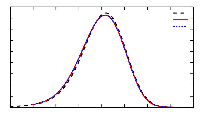
Figure 1: Comparison of density approximations. This figure shows transition density approximations of the Basic Affine Jump-Diffusion (BAJD) solving the stochastic differential equation dYt=(κθκYt)dt+σYtdWt+dLt𝑑subscript𝑌𝑡𝜅𝜃𝜅subscript𝑌𝑡𝑑𝑡𝜎subscript𝑌𝑡𝑑subscript𝑊𝑡𝑑subscript𝐿𝑡dY_{t}=(\kappa\theta-\kappa Y_{t})\,dt+\sigma\sqrt{Y_{t}}dW_{t}+dL_{t}. The parameters used are κθ=0.05,κ=1,σ=0.2,λ=1,ν=0.05,y0=0.05formulae-sequence𝜅𝜃0.05formulae-sequence𝜅1formulae-sequence𝜎0.2formulae-sequence𝜆1formulae-sequence𝜈0.05subscript𝑦00.05\kappa\theta=0.05,\kappa=1,\sigma=0.2,\lambda=1,\nu=0.05,y_{0}=0.05. Panels 1(a) and 1(b) show the approximation for a time span of Δ=3/12Δ312\Delta=3/12, and Δ=2/12Δ212\Delta=2/12, respectively. For both pictures, the exact density is obtained from Fourier inversion, while the density approximation FMS facilitates the approach from Filipović et al. (2013).

Figure 1 shows that the FMS density becomes negative close to zero, the more negative, the smaller ΔΔ\Delta, as Panels 1(a) and 1(b) indicate. Thus, in an application demanding positivity, such as derivatives pricing (Aït-Sahalia (1999)), likelihood ratio tests, or MCMC sampling, it is imperative to use the PLR proposed in this paper, rather than the FMS projections without modifications.

3.2 Distributions from options

Deviations from positivity of probability distributions may have sizable economic ramifications. In this section, we explore PLR in the context of option pricing and the concept of no-arbitrage. The absence of arbitrage, or free lunch, implies that any payoff Xt+Δsubscript𝑋𝑡ΔX_{t+\Delta} has forward price Ft(Xt+Δ)subscript𝐹𝑡subscript𝑋𝑡ΔF_{t}(X_{t+\Delta}), where Ftsubscript𝐹𝑡F_{t} is a linear operator that has a representation in terms of an expectation666We conduct our study in the forward market. Alternatively, in the spot market, we would assume zero interest rates for simplicity.

Ft(Xt+Δ)=𝔼𝒬[Xt+Δ|t],subscript𝐹𝑡subscript𝑋𝑡Δsuperscript𝔼𝒬delimited-[]conditionalsubscript𝑋𝑡Δsubscript𝑡F_{t}(X_{t+\Delta})=\mathbb{E}^{\mathcal{Q}}[X_{t+\Delta}|\mathcal{F}_{t}], (16)

where 𝒬𝒬\mathcal{Q} is a so-called forward measure. As before, we assume in this section that 𝒬𝒬\mathcal{Q} is absolutely continuous with respect to the Lebesgue measure with density q𝑞q (and likewise 𝒫𝒫\mathcal{P} with density p𝑝p). Note that here 𝒫𝒫\mathcal{P} represents an auxiliary possibly misspecified parametric probability measure approximating 𝒬𝒬\mathcal{Q}.

A call option written on the payoff Xt+Δsubscript𝑋𝑡ΔX_{t+\Delta} with strike price K𝐾K pays (Xt+ΔK)+superscriptsubscript𝑋𝑡Δ𝐾(X_{t+\Delta}-K)^{+}, while for puts the payoff is (KXt+Δ)+superscript𝐾subscript𝑋𝑡Δ(K-X_{t+\Delta})^{+}. Given a set 𝒦:={K1,,KΩ}assign𝒦subscript𝐾1subscript𝐾Ω\mathcal{K}:=\{K_{1},\ldots,K_{\Omega}\} of strike prices along with bid-ask spreads, or for simplicity, mid quotes of option forward prices Pt,Δ(K1),,Pt,Δ(Kω),Ct,Δ(Kω+1),,Ct,Δ(KΩ)subscript𝑃𝑡Δsubscript𝐾1subscript𝑃𝑡Δsubscript𝐾𝜔subscript𝐶𝑡Δsubscript𝐾𝜔1subscript𝐶𝑡Δsubscript𝐾ΩP_{t,\Delta}(K_{1}),\ldots,P_{t,\Delta}(K_{\omega}),C_{t,\Delta}(K_{\omega+1}),\ldots,C_{t,\Delta}(K_{\Omega}) of out-of-the-money options (meaning that K1<<KωFt(Xt+Δ)Kω+1<<KΩsubscript𝐾1subscript𝐾𝜔subscript𝐹𝑡subscript𝑋𝑡Δsubscript𝐾𝜔1subscript𝐾ΩK_{1}<\cdots<K_{\omega}\leq F_{t}(X_{t+\Delta})\leq K_{\omega+1}<\cdots<K_{\Omega}), our goal is to find a density q𝑞q that is compatible with these prices. If strike prices were continuously quoted, q𝑞q could be computed from second derivatives of option prices (Breeden and Litzenberger, 1978), but the presence of only a discrete observation 𝒦𝒦\mathcal{K} requires additional considerations to obtain q𝑞q.

Option cross sections are informative financial instruments, as from Carr and Madan (2001), for any twice-differentiable almost-everywhere function f𝑓f, its forward-neutral expectation is a particular option portfolio,

𝔼𝒬[f(Xt+Δ)|t]=0Ft(Xt+Δ)f′′(K)Pt,Δ(K)𝑑K+Ft(Xt+Δ)f′′(K)Ct,Δ(K)𝑑K,superscript𝔼𝒬delimited-[]conditional𝑓subscript𝑋𝑡Δsubscript𝑡superscriptsubscript0subscript𝐹𝑡subscript𝑋𝑡Δsuperscript𝑓′′𝐾subscript𝑃𝑡Δ𝐾differential-d𝐾superscriptsubscriptsubscript𝐹𝑡subscript𝑋𝑡Δsuperscript𝑓′′𝐾subscript𝐶𝑡Δ𝐾differential-d𝐾\mathbb{E}^{\mathcal{Q}}[f(X_{t+\Delta})|\mathcal{F}_{t}]=\int_{0}^{F_{t}(X_{t+\Delta})}f^{\prime\prime}(K)P_{t,\Delta}(K)dK+\int_{F_{t}(X_{t+\Delta})}^{\infty}f^{\prime\prime}(K)C_{t,\Delta}(K)dK, (17)

so that, for instance, forward-neutral moments can be approximated from observed option cross sections. We will use formula (17) to compute μi𝒬:=𝔼𝒬[(logXt+Δ)i|t]assignsuperscriptsubscript𝜇𝑖𝒬superscript𝔼𝒬delimited-[]conditionalsuperscriptsubscript𝑋𝑡Δ𝑖subscript𝑡\mu_{i}^{\mathcal{Q}}:=\mathbb{E}^{\mathcal{Q}}[(\log X_{t+\Delta})^{i}|\mathcal{F}_{t}] and σ𝒬:=μ2𝒬μ1𝒬assignsuperscript𝜎𝒬superscriptsubscript𝜇2𝒬superscriptsubscript𝜇1𝒬\sigma^{\mathcal{Q}}:=\sqrt{\mu_{2}^{\mathcal{Q}}-\mu_{1}^{\mathcal{Q}}} to define

Y:=logXt+ΔFt(Xt+Δ)μ1𝒬σ𝒬, and similarly w:=logKFt(Xt+Δ)μ1𝒬σ𝒬.formulae-sequenceassign𝑌subscript𝑋𝑡Δsubscript𝐹𝑡subscript𝑋𝑡Δsuperscriptsubscript𝜇1𝒬superscript𝜎𝒬assign and similarly 𝑤𝐾subscript𝐹𝑡subscript𝑋𝑡Δsuperscriptsubscript𝜇1𝒬superscript𝜎𝒬Y:=\frac{\log\frac{X_{t+\Delta}}{F_{t}(X_{t+\Delta})}-\mu_{1}^{\mathcal{Q}}}{\sigma^{\mathcal{Q}}},\text{ and similarly }w:=\frac{\log\frac{K}{F_{t}(X_{t+\Delta})}-\mu_{1}^{\mathcal{Q}}}{\sigma^{\mathcal{Q}}}. (18)

From this change of variables, forward option prices can be written as

Pt,Δ(K)=𝔼𝒬[(KXt+Δ)+]=eμ1𝒬Ft(Xt+Δ)logw(eσ𝒬weσ𝒬y)q~(y)𝑑y, andCt,Δ(K)=𝔼𝒬[(Xt+ΔK)+]=eμ1𝒬Ft(Xt+Δ)logw(eσ𝒬yeσ𝒬w)q~(y)𝑑y,formulae-sequencesubscript𝑃𝑡Δ𝐾superscript𝔼𝒬delimited-[]superscript𝐾subscript𝑋𝑡Δsuperscript𝑒superscriptsubscript𝜇1𝒬subscript𝐹𝑡subscript𝑋𝑡Δsuperscriptsubscript𝑤superscript𝑒superscript𝜎𝒬𝑤superscript𝑒superscript𝜎𝒬𝑦~𝑞𝑦differential-d𝑦 andsubscript𝐶𝑡Δ𝐾superscript𝔼𝒬delimited-[]superscriptsubscript𝑋𝑡Δ𝐾superscript𝑒superscriptsubscript𝜇1𝒬subscript𝐹𝑡subscript𝑋𝑡Δsuperscriptsubscript𝑤superscript𝑒superscript𝜎𝒬𝑦superscript𝑒superscript𝜎𝒬𝑤~𝑞𝑦differential-d𝑦\begin{split}P_{t,\Delta}(K)&=\mathbb{E}^{\mathcal{Q}}[(K-X_{t+\Delta})^{+}]=e^{\mu_{1}^{\mathcal{Q}}}F_{t}(X_{t+\Delta})\int_{-\infty}^{\log w}(e^{\sigma^{\mathcal{Q}}w}-e^{\sigma^{\mathcal{Q}}y})\tilde{q}(y)dy,\text{ and}\\ C_{t,\Delta}(K)&=\mathbb{E}^{\mathcal{Q}}[(X_{t+\Delta}-K)^{+}]=e^{\mu_{1}^{\mathcal{Q}}}F_{t}(X_{t+\Delta})\int_{\log w}^{\infty}(e^{\sigma^{\mathcal{Q}}y}-e^{\sigma^{\mathcal{Q}}w})\tilde{q}(y)dy,\end{split} (19)

where the density q~~𝑞\tilde{q} pertains to Y𝑌Y. From q~~𝑞\tilde{q}, we can recover the original density q𝑞q, the object of interest, from

q(x)=1xσQq~(logxFt(Xt+Δ)μ1QσQ).𝑞𝑥1𝑥superscript𝜎𝑄~𝑞𝑥subscript𝐹𝑡subscript𝑋𝑡Δsuperscriptsubscript𝜇1𝑄superscript𝜎𝑄q(x)=\frac{1}{x\,\sigma^{Q}}\tilde{q}\left(\frac{\log\frac{x}{F_{t}(X_{t+\Delta})}-\mu_{1}^{Q}}{\sigma^{Q}}\right).

The above centering and scaling facilitate the object of interest

ξn=q~pL𝒫2,subscript𝜉𝑛~𝑞𝑝subscriptsuperscript𝐿2𝒫\xi_{n}=\frac{\tilde{q}}{p}\in L^{2}_{\mathcal{P}},

such that the options are priced, and martingale and normalization restrictions, are satisfied. In terms of the auxiliary density p𝑝p, the martingale and density normalization restrictions that should be satisfied under the forward measure read

1=eμ1QeσQyξn(y)p(y)𝑑y, and 1=ξn(y)p(y)𝑑y, respectively.formulae-sequence1superscript𝑒superscriptsubscript𝜇1𝑄superscriptsubscriptsuperscript𝑒superscript𝜎𝑄𝑦subscript𝜉𝑛𝑦𝑝𝑦differential-d𝑦 and 1superscriptsubscriptsubscript𝜉𝑛𝑦𝑝𝑦differential-d𝑦 respectively\displaystyle 1=e^{\mu_{1}^{Q}}\int_{-\infty}^{\infty}e^{\sigma^{Q}y}\xi_{n}(y)p(y)dy,\text{ and }1=\int_{-\infty}^{\infty}\xi_{n}(y)p(y)dy,\text{ respectively}.

In the context of fat-tailed forward-neutral q~~𝑞\tilde{q} densities, the choice of the auxiliary density p𝑝p becomes particularly important. Lee (2004) investigates the tail of the distribution of forward-neutral log returns showing that it is exponential, and therefore ticker than the Gaussian tail. Thus, in the context of option pricing, the absolute continuity of p𝑝p with respect to q~~𝑞\tilde{q} puts strong restrictions on the choice of p𝑝p, excluding in particular the normal distribution, as its tails are too thin.

From these considerations, we solve the problem using the generalized hyperbolic distribution (Barndorff-Nielsen and Halgreen, 1977) as auxiliary density p𝑝p. The generalized hyperbolic distribution has four parameters. We choose the parameters to fit the first four moments of Y𝑌Y, such that μ1𝒬~=0,μ2𝒬~=1,μ3𝒬~,μ4𝒬~formulae-sequencesubscriptsuperscript𝜇~𝒬10subscriptsuperscript𝜇~𝒬21subscriptsuperscript𝜇~𝒬3subscriptsuperscript𝜇~𝒬4\mu^{\tilde{\mathcal{Q}}}_{1}=0,\mu^{\tilde{\mathcal{Q}}}_{2}=1,\mu^{\tilde{\mathcal{Q}}}_{3},\mu^{\tilde{\mathcal{Q}}}_{4}. These moments can be computed either from a model under consideration, or using formula (17) with observed option prices. Importantly, the generalized hyperbolic distribution features exponential tails, such that the approximation in L𝒫2subscriptsuperscript𝐿2𝒫L^{2}_{\mathcal{P}} is meaningful. In particular, for the parameterizations used below, the tails of the generalized hyperbolic distribution satisfy the L𝒫2subscriptsuperscript𝐿2𝒫L^{2}_{\mathcal{P}} integrability condition.

Specializing program (6) for the task of extracting a density from option prices, we

minimize ξnMn(D)ξn2, subject to (ξn,1)=1,(ξn,eμ1QeσQY)=1,1ε(ξn,eμ1QFt(Xt+Δ)(eσQwjeσQY)+PΔ(Kj))1+ε,j=1,,ω1ε(ξn,eμ1QFt(Xt+Δ)(eσQYeσQwj)+CΔ(Kj))1+ε,j=ω+1,,Ωformulae-sequencesubscript𝜉𝑛subscript𝑀𝑛𝐷minimize superscriptdelimited-∥∥subscript𝜉𝑛2 subject to subscript𝜉𝑛11formulae-sequencesubscript𝜉𝑛superscript𝑒superscriptsubscript𝜇1𝑄superscript𝑒superscript𝜎𝑄𝑌11𝜀subscript𝜉𝑛superscript𝑒superscriptsubscript𝜇1𝑄subscript𝐹𝑡subscript𝑋𝑡Δsuperscriptsuperscript𝑒superscript𝜎𝑄subscript𝑤𝑗superscript𝑒superscript𝜎𝑄𝑌subscript𝑃Δsubscript𝐾𝑗1𝜀formulae-sequence𝑗1𝜔1𝜀subscript𝜉𝑛superscript𝑒superscriptsubscript𝜇1𝑄subscript𝐹𝑡subscript𝑋𝑡Δsuperscriptsuperscript𝑒superscript𝜎𝑄𝑌superscript𝑒superscript𝜎𝑄subscript𝑤𝑗subscript𝐶Δsubscript𝐾𝑗1𝜀𝑗𝜔1Ω\begin{split}&\underset{\xi_{n}\in M_{n}(D)}{\text{minimize }}\left\|\xi_{n}\right\|^{2},\\ &\text{ subject to }(\xi_{n},1)=1,\,(\xi_{n},e^{\mu_{1}^{Q}}e^{\sigma^{Q}\cdot Y})=1,\\ &1-\varepsilon\leq\left(\xi_{n},\frac{e^{\mu_{1}^{Q}}F_{t}(X_{t+\Delta})(e^{\sigma^{Q}\cdot w_{j}}-e^{\sigma^{Q}\cdot Y})^{+}}{P_{\Delta}(K_{j})}\right)\leq 1+\varepsilon,\,j=1,\ldots,\omega\\ &1-\varepsilon\leq\left(\xi_{n},\frac{e^{\mu_{1}^{Q}}F_{t}(X_{t+\Delta})(e^{\sigma^{Q}\cdot Y}-e^{\sigma^{Q}\cdot w_{j}})^{+}}{C_{\Delta}(K_{j})}\right)\leq 1+\varepsilon,\,j=\omega+1,\ldots,\Omega\end{split} (20)

Tolerance ε>0𝜀0\varepsilon>0 bounds the maximal relative option pricing error from above. Lu and Qu (2021) perform a similar task with polynomials by minimizing the squared pricing errors. Differently from their approach, we obtain a positive density q𝑞q, that furthermore satisfies the martingale restriction (ξn,eμ1QeσQY)=1subscript𝜉𝑛superscript𝑒superscriptsubscript𝜇1𝑄superscript𝑒superscript𝜎𝑄𝑌1(\xi_{n},e^{\mu_{1}^{Q}}e^{\sigma^{Q}\cdot Y})=1. Additionally, the generalized hyperbolic distribution features exponential tails, while Lu and Qu (2021) employ the normal distribution, for which the approximating expansion diverges asymptotically.

We illustrate our approach using the Duffie et al. (2000) double-jump model for logXtsubscript𝑋𝑡\log X_{t}, and its stochastic variance process Vtsubscript𝑉𝑡V_{t} with joint dynamics

d(logXtVt)=(rλ¯μ¯12Vtκv(v¯Vt))dt+Vt(ρ1ρ2σv0)d(W1,tqW2,tq)+dJtQ,𝑑matrixsubscript𝑋𝑡subscript𝑉𝑡matrix𝑟¯𝜆¯𝜇12subscript𝑉𝑡subscript𝜅𝑣¯𝑣subscript𝑉𝑡𝑑𝑡subscript𝑉𝑡matrix𝜌1superscript𝜌2subscript𝜎𝑣0𝑑matrixsubscriptsuperscript𝑊𝑞1𝑡subscriptsuperscript𝑊𝑞2𝑡𝑑subscriptsuperscript𝐽𝑄𝑡d\begin{pmatrix}\log X_{t}\\ V_{t}\end{pmatrix}=\begin{pmatrix}r-\bar{\lambda}\bar{\mu}-\frac{1}{2}V_{t}\\ \kappa_{v}(\bar{v}-V_{t})\end{pmatrix}dt+\sqrt{V_{t}}\begin{pmatrix}\rho&\sqrt{1-\rho^{2}}\\ \sigma_{v}&0\end{pmatrix}d\begin{pmatrix}W^{q}_{1,t}\\ W^{q}_{2,t}\end{pmatrix}+dJ^{Q}_{t}, (21)

where W1,t𝒬,W2,t𝒬subscriptsuperscript𝑊𝒬1𝑡subscriptsuperscript𝑊𝒬2𝑡W^{\mathcal{Q}}_{1,t},W^{\mathcal{Q}}_{2,t} are 𝒬𝒬\mathcal{Q} Brownian motions, and J𝒬superscript𝐽𝒬J^{\mathcal{Q}} is a pure jump process in 2superscript2\mathbb{R}^{2} with constant mean arrival rate λ¯¯𝜆\bar{\lambda}, and μ¯¯𝜇\bar{\mu} is the mean jump size in the logXtsubscript𝑋𝑡\log X_{t} direction under 𝒬𝒬\mathcal{Q}.

For fixed ΔΔ\Delta, the characteristic function of logXt+Δ,Vt+Δ|logXt,Vtsubscript𝑋𝑡Δconditionalsubscript𝑉𝑡Δsubscript𝑋𝑡subscript𝑉𝑡\log X_{t+\Delta},V_{t+\Delta}|\log X_{t},V_{t} is readily available in closed form, such that option prices can be obtained via the dampened transform as proposed by Lee (2004). Using the estimated parameters from Duffie et al. (2000, TABLE I), we consider three scenarios for the value of Vtsubscript𝑉𝑡V_{t}: low (Vt=0.02subscript𝑉𝑡0.02\sqrt{V_{t}}=0.02), medium (Vt=0.087subscript𝑉𝑡0.087\sqrt{V_{t}}=0.087, the value quoted in the original paper), and high (Vt=0.17subscript𝑉𝑡0.17\sqrt{V_{t}}=0.17), and compute the resulting densities with positivity restriction, and without. For both the positive and the unrestricted PLR we find the smallest possible tolerance ε𝜀\varepsilon that makes program (20) feasible through trial and error. This process takes a fraction of a second.
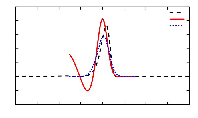
2020-201010-10001010102020203030304040405050500.20.2-0.20.150.15-0.150.10.1-0.10.050.05-0.05000.050.050.050.10.10.10.150.150.150.20.20.2Refer to captiontrueno restr.pos.
(a) Transition density, low volatility
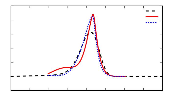
55-5005551010101515152020202525250.20.2-0.20.150.15-0.150.10.1-0.10.050.05-0.05000.050.050.050.10.10.10.150.150.150.20.20.2Refer to captiontrueno restr.pos.
(b) Transition density, medium volatility
001112223334445556667778889990.20.2-0.20.150.15-0.150.10.1-0.10.050.05-0.05000.050.050.050.10.10.10.150.150.150.20.20.2Refer to captiontrueno restr.pos.
(c) Transition density, high volatility
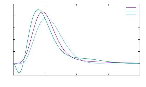
Figure 2: Densities implied from options. The figure shows the true density, the density solving program (20) without (no restr.), and with (pos.) positivity restriction for the Duffie et al. (2000) double-jump model estimated from options. Option data is generated for low (Vt=0.02subscript𝑉𝑡0.02\sqrt{V_{t}}=0.02), medium (Vt=0.087subscript𝑉𝑡0.087\sqrt{V_{t}}=0.087), and high (Vt=0.17subscript𝑉𝑡0.17\sqrt{V_{t}}=0.17) volatility at valuation time. Both types of PLR are computed with polynomial degree n=8𝑛8n=8. In the horizontal axis we observe log returns logXt+ΔXt𝑙𝑜𝑔subscript𝑋𝑡Δsubscript𝑋𝑡log\frac{X_{t+\Delta}}{X_{t}} of the underlying asset.

Figure 2 shows transition densities computed from Fourier inversion of model-implied option prices (true), without (no restr.), and with (pos.) positivity restriction imposed when solving program (20). Panels 2(a) and 2(c) show reasonably accurate q𝑞q densities for the low and high volatility scenarios, while the medium volatility in Panel 2(b) scenario is estimated too peaked. The reason for this is the auxiliary generalized hyperbolic distribution p𝑝p, which despite matching the first four moments of the original distribution q~~𝑞\tilde{q}, features a peak that an order eight polynomial can not tilt sufficiently. Note that the unrestricted transition density achieves large negative values for negative returns close to zero.
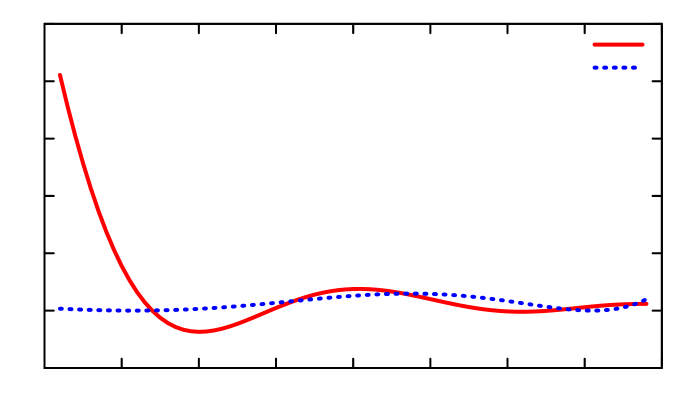
55-5005551010101515152020202525250.080.08-0.080.060.06-0.060.040.04-0.040.020.02-0.02000.020.020.020.040.040.040.060.060.060.080.080.08Refer to captionno restr.pos.
(a) ξnsubscript𝜉𝑛\xi_{n}, low volatility
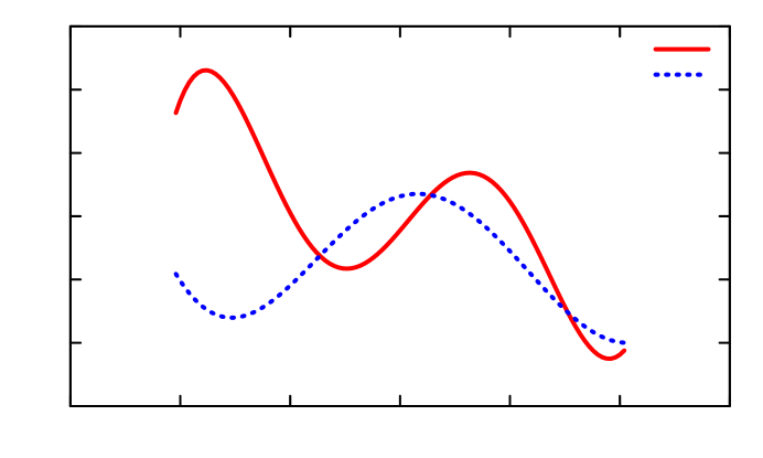
0.50.5-0.5000.50.50.51111.51.51.52222.52.52.50.150.15-0.150.10.1-0.10.050.05-0.05000.050.050.050.10.10.10.150.150.15Refer to captionno restr.pos.
(b) ξnsubscript𝜉𝑛\xi_{n}, medium volatility
0.50.50.50.60.60.60.70.70.70.80.80.80.90.90.91111.11.11.10.20.2-0.20.150.15-0.150.10.1-0.10.050.05-0.05000.050.050.050.10.10.10.150.150.150.20.20.2Refer to captionno restr.pos.
(c) ξnsubscript𝜉𝑛\xi_{n}, high volatility
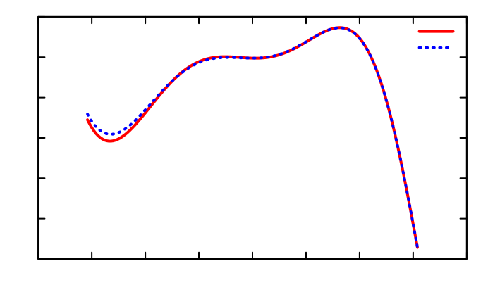
Figure 3: Polynomial tilts. The figure shows the resulting polynomial ξnsubscript𝜉𝑛\xi_{n} from the solution of the program (20) without (no restr.), and with (pos.) positivity restriction for the Duffie et al. (2000) double-jump model estimated from options. Option data is generated for low (Vt=0.02subscript𝑉𝑡0.02\sqrt{V_{t}}=0.02), medium (Vt=0.087subscript𝑉𝑡0.087\sqrt{V_{t}}=0.087), and high (Vt=0.17subscript𝑉𝑡0.17\sqrt{V_{t}}=0.17) volatility at valuation time. Both types of PLR are computed with polynomial degree n=8𝑛8n=8. In the horizontal axis we observe log returns logXt+ΔXt𝑙𝑜𝑔subscript𝑋𝑡Δsubscript𝑋𝑡log\frac{X_{t+\Delta}}{X_{t}} of the underlying asset.

Figure 3 illustrates the stark differences between the unrestricted PLR and the positive one induced by the positivity condition. It also shows that the tilting is moderate in magnitude, thanks to the minimum-norm objective function. The unrestricted ξnsubscript𝜉𝑛\xi_{n}, i.e., the one with no positivity restriction, takes negative values for all scenarios but the high-volatility one and presents an excessive oscillatory behavior when volatility is low or medium.
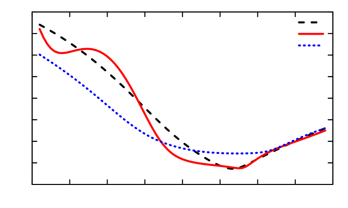
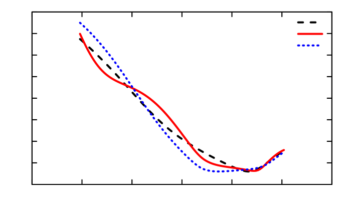
0.020.020.020.040.040.040.060.060.060.080.080.080.10.10.10.120.120.120.140.140.140.160.160.160.180.180.180.080.08-0.080.060.06-0.060.040.04-0.040.020.02-0.02000.020.020.020.040.040.040.060.060.060.080.080.08Refer to captiontrueno restr.pos.
(a) Implied volatility, low volatility
0.060.060.060.080.080.080.10.10.10.120.120.120.140.140.140.160.160.160.180.180.180.20.20.20.220.220.220.150.15-0.150.10.1-0.10.050.05-0.05000.050.050.050.10.10.10.150.150.15Refer to captiontrueno restr.pos.
(b) Implied volatility, medium volatility
0.120.120.120.140.140.140.160.160.160.180.180.180.20.20.20.220.220.220.240.240.240.260.260.260.20.2-0.20.150.15-0.150.10.1-0.10.050.05-0.05000.050.050.050.10.10.10.150.150.150.20.20.2Refer to captiontrueno restr.pos.
(c) Implied volatility, high volatility
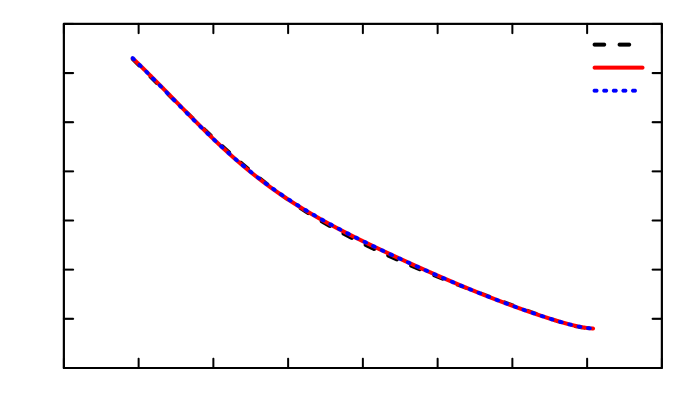
Figure 4: Comparison of implied volatilities. The figure shows Black-Scholes implied volatilities of the option prices generated by the true distribution (true), the density solving program (20) without (no restr.), and with (pos.) positivity restriction for the Duffie et al. (2000) double-jump model estimated from options as a function of log moneyness. Option data is generated for low (Vt=0.02subscript𝑉𝑡0.02\sqrt{V_{t}}=0.02), medium (Vt=0.087subscript𝑉𝑡0.087\sqrt{V_{t}}=0.087), and high (Vt=0.17subscript𝑉𝑡0.17\sqrt{V_{t}}=0.17) volatility at valuation time. Both types of PLR are computed with polynomial degree n=8𝑛8n=8. In the horizontal axis we observe log moneyness logKXt𝑙𝑜𝑔𝐾subscript𝑋𝑡log\frac{K}{X_{t}}.

Figure 4 shows Black-Scholes implied volatilities from the true model, as well as the polynomial approximations. From Panel 4(a) it becomes apparent that the low volatility scenario is the most challenging. In this scenario, OTM call options have low prices dominating the relative pricing error on both polynomial likelihood approximations what forces them to sacrifice part of their ability to price OTM puts. The consequences for the implied volatility curve is that both models underprice puts (negative log-moneyness in the picture) with the unconstrained model having smaller bias and an intermediary region of log-moneyness where it overprices puts. The positive model trades precision to avoid the excessive oscillatory behavior produced by the unconstrained PLR on the implied volatility curve, which comes from the oscillatory behavior of its estimated transition density noted in Figure 2. This excessive oscillatory behavior of implied volatilities also appears in the medium volatility scenario for the unconstrained model, contrasting with well-behaved implied volatilities under positivity constrain. Finally, note that both approximations work quite well in the high volatility scenario.

4 Conclusion

We develop projections of likelihood ratios onto polynomials that preserve positivity. We term them positive polynomial likelihood ratio (PLR). PLR can accommodate shape restrictions, are fast and robust to compute as solutions to conic programs, and come with asymptotic theory for their use with sample moments.

We illustrate PLR with two applications. The first is an approximation of the unknown transition density of a jump-diffusion process. The second construct a density from the observation of option prices only. In both cases, the virtue of positivity of the PLR becomes evident through the positivity of the resulting distributions, that without the restriction, becomes negative and with excessive oscillatory behavior.

PLR lend themselves to nonparametric structurally constrained settings, such as for instance Christensen (2017) discount factor decomposition. We leave this, and related applications to future research.

References

  • Aït-Sahalia [1999] Yacine Aït-Sahalia. Transition densities for interest rate and other nonlinear diffusions. Journal of Finance, 54(4):1361–1395, 1999.
  • Aït-Sahalia [2002] Yacine Aït-Sahalia. Maximum likelihood estimation of discretely-sampled diffusions: a closed-form approximation approach. Econometrica, 70:223–262, 2002.
  • Aït-Sahalia and Yu [2006] Yacine Aït-Sahalia and Jialin Yu. Saddlepoint approximations for continuous-time Markov processes. Journal of Econometrics, 134:507–551, 2006.
  • Alvarez and Jermann [2005] Fernando Alvarez and Urban Jermann. Using asset prices to measure the persistence of the marginal utility of wealth. Econometrica, 73:1977–2016, 2005.
  • Backus et al. [2014] David K. Backus, Mikhail Chernov, and Stanley Zin. Affine term structure models and the forward premium anomaly. Journal of Finance, 69(1):51–99, February 2014.
  • Barndorff-Nielsen and Halgreen [1977] O. Barndorff-Nielsen and C. Halgreen. Infinite divisibility of the hyperbolic and generalized inverse gaussian distributions. Zeitschrift für Wahrscheinlichkeitstheorie und verwandte Gebiete, 38:309–311, 1977.
  • Bates [2000] David S. Bates. Post-’87 crash fears in the s&p 500 futures option market. Journal of Econometrics, 94(1-2):181–238, 2000.
  • Berlinet and Thomas-Agnan [2004] Alain Berlinet and Christine Thomas-Agnan. Reproducing Kernel Hilbert Spaces in Probability and Statistics, pages 1–54. Springer US, Boston, MA, 2004.
  • Borovička et al. [2016] Jaroslav Borovička, Lars Peter Hansen, and José A. Scheinkman. Misspecified recovery. Journal of Finance, 71:2493–2544, 2016.
  • Breeden and Litzenberger [1978] Douglas T. Breeden and Robert H. Litzenberger. Prices of state-contingent claims implicit in option prices. Journal of Business, 51:621–651, 1978.
  • Brigo and Mercurio [2006] Damiano Brigo and Fabio Mercurio. Interest Rate Models: Theory and Practice. With Smile, Inflation and Credit. Springer-Verlag, 2006.
  • Carr and Madan [2001] Peter Carr and Dilip Madan. Towards a theory of volatility trading. Option Pricing, Interest Rates and Risk Management, pages 458–476. Cambridge University Press, New York, 2001.
  • Chabi-Yo and Bakshi [2012] Fousseni Chabi-Yo and Gurdip Bakshi. Variance bounds on the permanent and transitory components of the stochastic discount factor. Journal of Financial Economics, 105(1):191–208, 2012.
  • Chabi-Yo et al. [2015] Fousseni Chabi-Yo, Gurdip Bakshi, and Xiaohui Gao. A recovery that we can trust? deducing and testing the restrictions of the recovery theorem. Working paper, University of Maryland, and Fisher College of Business, 2015.
  • Chen [2007] Xiaohong Chen. Large sample sieve estimation of semi-nonparametric models. Handbook of Econometrics, edited by Heckman, J. and E.E. Leamer, 6(B):5549–5632, 2007.
  • Christensen [2017] Timothy Christensen. Nonparametric stochastic discount factor decomposition. Econometrica, 85(5):1501–1536, 2017.
  • Duffie et al. [2000] Darrell Duffie, Jun Pan, and Kenneth Singleton. Transform analysis and asset pricing for affine jump-diffusions. Econometrica, 68:1343–1376, 2000.
  • Duffie et al. [2003] Darrell Duffie, Damir Filipović, and Walter Schachermayer. Affine processes and applications in finance. Annals of Applied Probability, 13:984–1053, 2003.
  • Filipović et al. [2013] Damir Filipović, Eberhard Mayerhofer, and Paul Schneider. Density approximations for multivariate affine jump-diffusion processes. Journal of Econometrics, 176:93–111, 2013.
  • Giesecke and Schwenkler [2018] Kay Giesecke and Gustavo Schwenkler. Filtered likelihood for point processes. Journal of Econometrics, 204(1):33 – 53, 2018. ISSN 0304-4076.
  • Grenander [1981] U. Grenander. Abstract inference / Ulf Grenander. Wiley New York, 1981. ISBN 0471082678.
  • Grünewälder et al. [2012] Steffen Grünewälder, Guy Lever, Luca Baldassarre, Sam Patterson, Arthur Gretton, and Massimilano Pontil. Conditional mean embeddings as regressors. ICML’12, pages 1803–1810. Omnipress, 2012. ISBN 9781450312851.
  • Hansen and Scheinkman [2009] Lars Peter Hansen and José Scheinkman. Long-term risk: An operator approach. Econometrica, 77:177–234, 2009.
  • Kato and Kuriki [2013] Naohiro Kato and Satoshi Kuriki. Likelihood ratio tests for positivity in polynomial regressions. Journal of Multivariate Analysis, 115:334–346, 2013.
  • Klebanov et al. [2020] Ilja Klebanov, Ingmar Schuster, and T.J. Sullivan. A rigorous theory of conditional mean embeddings. SIAM Journal on Mathematics of Data Science, 2(3):583–606, 2020.
  • Lee [2004] Roger Lee. Option pricing by transform methods: extensions, unification and error control. 7:51–86, 2004.
  • Lu and Qu [2021] Junwen Lu and Zhongjun Qu. Sieve estimation of option-implied state price density. Journal of Econometrics, 224(1):88–112, 2021. ISSN 0304-4076. doi: https://doi.org/10.1016/j.jeconom.2021.03.003. URL https://www.sciencedirect.com/science/article/pii/S0304407621000737. Annals Issue: PI Day.
  • Luenberger [1997] David G. Luenberger. Optimization by Vector Space Methods. John Wiley & Sons, Inc., New York, NY, USA, 1st edition, 1997. ISBN 047118117X.
  • Mijatović and Schneider [2010] Aleksandar Mijatović and Paul Schneider. Globally optimal parameters for non-linear diffusions. Annals of Statistics, 38(1):215–245, 2010.
  • Park and Muandet [2020] Junhyung Park and Krikamol Muandet. A measure-theoretic approach to kernel conditional mean embeddings. Working paper, Max Planck Institute for Intelligent Systems, 2020.
  • Qin and Linetsky [2016] Likuan Qin and Vadim Linetsky. Positive eigenfunctions of Markovian pricing operators: Hansen-Scheinkman factorization, Ross recovery, and long-term pricing. Operations Research, 64:99–117, 2016.
  • Qin and Linetsky [2017] Likuan Qin and Vadim Linetsky. Long-term risk: A martingale approach. Econometrica, 85:299–312, 2017.
  • Renner and Schmedders [2015] Philipp Renner and Karl Schmedders. A polynomial optimization approach to principal-agent problems. Econometrica, 83:729–769, 2015.
  • Ross [2015] Steve Ross. The recovery theorem. Journal of Finance, 70:615–648, 2015.
  • Schmüdgen [2017] Konrad Schmüdgen. The Moment Problem. Graduate Texts in Mathematics. Springer International Publishing, 2017. ISBN 9783319645469.
  • Schuster et al. [2020] Ingmar Schuster, Mattes Mollenhauer, Stefan Klus, and Krikamol Muandet. Kernel conditional density operators. volume 108 of Proceedings of Machine Learning Research, pages 993–1004, Online, 26–28 Aug 2020. PMLR.
  • Song et al. [2009] Le Song, Jonathan Huang, Alex Smola, and Kenji Fukumizu. Hilbert space embeddings of conditional distributions with applications to dynamical systems. In Proceedings of the 26th Annual International Conference on Machine Learning, ICML 2009, pages 961–968, New York, NY, USA, 2009. Association for Computing Machinery. ISBN 9781605585161.
  • Yu [2007] Jialin Yu. Closed-form likelihood estimation of jump-diffusions with an application to the realignment risk of the chinese yuan. Journal of Econometrics, 141:1245–1280, 2007.
\appendixpage

Appendix A Positive polynomials

In this section, we review results in the literature about positive polynomials. In the univariate case, we have

Proposition A1 (Schmüdgen [2017]).

For any positive integer n𝑛n,

  1. 1.

    D=𝐷D=\mathbb{R}: Ωn:=M2n={f2(t)+g2(t):f,g[t]n}assignsubscriptΩ𝑛subscript𝑀2𝑛conditional-setsuperscript𝑓2𝑡superscript𝑔2𝑡𝑓𝑔subscriptdelimited-[]𝑡𝑛\Omega_{n}:=M_{2n}=\left\{f^{2}(t)+g^{2}(t):f,g\in\mathbb{R}[t]_{n}\right\},

  2. 2.

    D=+𝐷subscriptD=\mathbb{R}_{+}: M2n={f(t)+tg(t):fΩn,gΩn1}subscript𝑀2𝑛conditional-set𝑓𝑡𝑡𝑔𝑡formulae-sequence𝑓subscriptΩ𝑛𝑔subscriptΩ𝑛1M_{2n}=\left\{f(t)+tg(t):f\in\Omega_{n},g\in\Omega_{n-1}\right\},

  3. 3.

    D=+𝐷subscriptD=\mathbb{R}_{+}: M2n+1={f(t)+tg(t):f,gΩn}subscript𝑀2𝑛1conditional-set𝑓𝑡𝑡𝑔𝑡𝑓𝑔subscriptΩ𝑛M_{2n+1}=\left\{f(t)+tg(t):f,g\in\Omega_{n}\right\},

  4. 4.

    D=[a,b]𝐷𝑎𝑏D=[a,b]: M2n={f(t)+(bt)(ta)g(t):fΩn,gΩn1}subscript𝑀2𝑛conditional-set𝑓𝑡𝑏𝑡𝑡𝑎𝑔𝑡formulae-sequence𝑓subscriptΩ𝑛𝑔subscriptΩ𝑛1M_{2n}=\left\{f(t)+(b-t)(t-a)g(t):f\in\Omega_{n},g\in\Omega_{n-1}\right\},

  5. 5.

    D=[a,b]𝐷𝑎𝑏D=[a,b]: M2n+1={(bt)f(t)+(ta)g(t):f,gΩn}subscript𝑀2𝑛1conditional-set𝑏𝑡𝑓𝑡𝑡𝑎𝑔𝑡𝑓𝑔subscriptΩ𝑛M_{2n+1}=\left\{(b-t)f(t)+(t-a)g(t):f,g\in\Omega_{n}\right\}.

The set of positive polynomials on any other (continuous) state space can be extracted from Proposition A1 from a change of variables. For instance, D=[a,)𝐷𝑎D=[a,\infty) can be obtained from parameterization (2) above through the change of variables p(ta)𝑝𝑡𝑎p(t-a) for pM2n𝑝subscript𝑀2𝑛p\in M_{2n} on D=+𝐷subscriptD=\mathbb{R}_{+}.

In the multivariate case, nonnegative polynomials exist that are not s.o.s.. Since we merely want to assure non-negativity, and a s.o.s. polynomial is certainly non-negative, it is sufficient for our purpose to work with s.o.s. polynomials. Any such polynomial has a representation as a quadratic form (the proof is in Schmüdgen [2017] for Proposition 13.2).

Proposition A2.

A polynomial ξ2n[t]2nsubscript𝜉2𝑛subscriptdelimited-[]𝑡2𝑛\xi_{2n}\in\mathbb{R}[t]_{2n} is s.o.s. if and only if ξ2n=τn𝐕τn, with 𝐕0.formulae-sequencesubscript𝜉2𝑛superscriptsubscript𝜏𝑛top𝐕subscript𝜏𝑛succeeds-or-equals with 𝐕0\xi_{2n}=\tau_{n}^{\top}\,\bm{V}\,\tau_{n},\text{ with }\bm{V}\succeq 0.

Note that we do not make a distinction between different supports in the multivariate case. Statements A1 and A2 lead to our parameterization 2.1 of the cone of positive polynomials.

Appendix B Proofs

Proposition 2.4

Proof.

For the minimization, it is convenient to use one-half the squared norm as an objective function rather than the norm itself. This does not change the result, since the norm is non-negative, and we can write

ξn2/2=12(ξn,ξn)=12D𝒙𝝉n(t)𝝉n(t)𝒙𝑑𝒫(t)=12𝒙𝑯n𝒙.superscriptnormsubscript𝜉𝑛2212subscript𝜉𝑛subscript𝜉𝑛12subscript𝐷superscript𝒙topsubscript𝝉𝑛𝑡superscriptsubscript𝝉𝑛top𝑡𝒙differential-d𝒫𝑡12superscript𝒙topsubscript𝑯𝑛𝒙\left\|\xi_{n}\right\|^{2}/2=\frac{1}{2}(\xi_{n},\xi_{n})=\frac{1}{2}\int_{D}\bm{x}^{\top}\bm{\tau}_{n}(t)\bm{\tau}_{n}^{\top}(t)\bm{x}\,d\mathcal{P}(t)=\frac{1}{2}\bm{x}^{\top}\bm{H}_{n}\bm{x}.

Together with the constraints in coordinate form and Proposition A2, this yields primal (8) that can be solved as a mixed conic semidefinite program.777We use the Mosek optimizer to solve the program in practice. Since with Assumption 2.2 the objective function is strictly convex, and the constraint set is an intersection of closed convex sets, the solution with Assumption 2.3 is unique in 𝒙𝒙\bm{x}, and strong duality obtains. With strong duality at hand, we next consider the dual form to (8). Furthermore, the cone of symmetric positive semidefinite matrix is self-dual. From these observations, we can write the Lagrangian of system (8) as

(𝒙,𝜼,𝝂,𝜺,𝚲V,𝚲W)𝒙𝜼𝝂𝜺subscript𝚲𝑉subscript𝚲𝑊\displaystyle\mathcal{L}(\bm{x},\bm{\eta},\bm{\nu},\bm{\varepsilon},\bm{\Lambda}_{V},\bm{\Lambda}_{W}) :=12𝒙𝑯n𝒙𝜼(𝑭n𝒙𝒄)𝝂(𝒙T(𝑽,𝑾))assignabsent12superscript𝒙topsubscript𝑯𝑛𝒙superscript𝜼topsubscript𝑭𝑛𝒙𝒄superscript𝝂top𝒙𝑇𝑽𝑾\displaystyle:=\frac{1}{2}\bm{x}^{\top}\bm{H}_{n}\bm{x}-\bm{\eta}^{\top}(\bm{F}_{n}\bm{x}-\bm{c})-\bm{\nu}^{\top}(\bm{x}-T(\bm{V},\bm{W})) (22)
+𝜺(𝑮n𝒙𝒅)tr(𝚲V𝑽)tr(𝚲W𝑾)superscript𝜺topsubscript𝑮𝑛𝒙𝒅trsubscript𝚲𝑉𝑽trsubscript𝚲𝑊𝑾\displaystyle+\bm{\varepsilon}^{\top}(\bm{G}_{n}\bm{x}-\bm{d})-\operatorname{tr}(\bm{\Lambda}_{V}\bm{V})-\operatorname{tr}(\bm{\Lambda}_{W}\bm{W})

for 𝜼m,𝜺+l,𝝂N+1formulae-sequence𝜼superscript𝑚formulae-sequence𝜺superscriptsubscript𝑙𝝂superscript𝑁1\bm{\eta}\in\mathbb{R}^{m},\bm{\varepsilon}\in\mathbb{R}_{+}^{l},\bm{\nu}\in\mathbb{R}^{N+1}, as well as p.s.d. matrices 𝝀V,𝝀Wsubscript𝝀𝑉subscript𝝀𝑊\bm{\lambda}_{V},\bm{\lambda}_{W} of the same dimension as 𝑽𝑽\bm{V} and 𝑾𝑾\bm{W}, respectively. From the first-order condition (on 𝒙𝒙\bm{x}) we can then deduce 𝒙0𝑯n𝜼0𝑭n𝝂0+𝜺0𝑮n=0superscriptsubscript𝒙0topsubscript𝑯𝑛subscriptsuperscript𝜼top0subscript𝑭𝑛subscriptsuperscript𝝂top0subscriptsuperscript𝜺top0subscript𝑮𝑛0\bm{x}_{0}^{\top}\bm{H}_{n}-\bm{\eta}^{\top}_{0}\bm{F}_{n}-\bm{\nu}^{\top}_{0}+\bm{\varepsilon}^{\top}_{0}\bm{G}_{n}=0, and with 𝑯nsubscript𝑯𝑛\bm{H}_{n} invertible from Assumption 2.2, any optimal solution must satisfy (11). The Lagrangian is linear-quadratic in 𝑽𝑽\bm{V} and 𝑾𝑾\bm{W}, and taking matrix derivatives, we therefore have the conditions ν0𝑽0++νN𝑽N=𝚲V0subscript𝜈0subscript𝑽0subscript𝜈𝑁subscript𝑽𝑁subscript𝚲𝑉succeeds-or-equals0\nu_{0}\bm{V}_{0}+\cdots+\nu_{N}\bm{V}_{N}=\bm{\Lambda}_{V}\succeq 0, and analogously ν0𝑾0++νN𝑾N=𝚲W0subscript𝜈0subscript𝑾0subscript𝜈𝑁subscript𝑾𝑁subscript𝚲𝑊succeeds-or-equals0\nu_{0}\bm{W}_{0}+\cdots+\nu_{N}\bm{W}_{N}=\bm{\Lambda}_{W}\succeq 0. Plugging these relations into the Lagrangian yields

g(𝜼,𝝂,𝜺)𝑔𝜼𝝂𝜺\displaystyle g(\bm{\eta},\bm{\nu},\bm{\varepsilon}) =12(𝜼𝑭n+𝝂𝜺𝑮n)𝑯n1(𝑭n𝜼+𝝂𝑮n𝜺)absent12superscript𝜼topsubscript𝑭𝑛superscript𝝂topsuperscript𝜺topsubscript𝑮𝑛superscriptsubscript𝑯𝑛1superscriptsubscript𝑭𝑛top𝜼𝝂superscriptsubscript𝑮𝑛top𝜺\displaystyle=\frac{1}{2}(\bm{\eta}^{\top}\bm{F}_{n}+\bm{\nu}^{\top}-\bm{\varepsilon}^{\top}\bm{G}_{n})\bm{H}_{n}^{-1}(\bm{F}_{n}^{\top}\bm{\eta}+\bm{\nu}-\bm{G}_{n}^{\top}\bm{\varepsilon})
𝜼(𝑭n𝑯n1(𝑭n𝜼+𝝂𝑮n𝜺)𝒄)superscript𝜼topsubscript𝑭𝑛superscriptsubscript𝑯𝑛1superscriptsubscript𝑭𝑛top𝜼𝝂superscriptsubscript𝑮𝑛top𝜺𝒄\displaystyle-\bm{\eta}^{\top}(\bm{F}_{n}\bm{H}_{n}^{-1}(\bm{F}_{n}^{\top}\bm{\eta}+\bm{\nu}-\bm{G}_{n}^{\top}\bm{\varepsilon})-\bm{c})
𝝂𝑯n1(𝑭n𝜼+𝝂𝑮n𝜺)superscript𝝂topsuperscriptsubscript𝑯𝑛1superscriptsubscript𝑭𝑛top𝜼𝝂superscriptsubscript𝑮𝑛top𝜺\displaystyle-\bm{\nu}^{\top}\bm{H}_{n}^{-1}(\bm{F}_{n}^{\top}\bm{\eta}+\bm{\nu}-\bm{G}_{n}^{\top}\bm{\varepsilon})
+𝜺(𝑮n𝑯n1(𝑭n𝜼+𝝂𝑮n𝜺)𝒅).superscript𝜺topsubscript𝑮𝑛superscriptsubscript𝑯𝑛1superscriptsubscript𝑭𝑛top𝜼𝝂superscriptsubscript𝑮𝑛top𝜺𝒅\displaystyle+\bm{\varepsilon}^{\top}(\bm{G}_{n}\bm{H}_{n}^{-1}(\bm{F}_{n}^{\top}\bm{\eta}+\bm{\nu}-\bm{G}_{n}^{\top}\bm{\varepsilon})-\bm{d}).

The objective function in (8) can be obtained by completing the square. ∎

Proposition 2.6

Proof.

In this section, we denote by \|\cdot\| the Euclidean norm for lighter notation (rather than the L𝒫2subscriptsuperscript𝐿2𝒫L^{2}_{\mathcal{P}} norm). For convenience, define k(𝒙):=𝒙𝑯^n,k𝒙assignsubscript𝑘𝒙superscript𝒙topsubscript^𝑯𝑛𝑘𝒙\mathcal{R}_{k}(\bm{x}):=\bm{x}^{\top}\hat{\bm{H}}_{n,k}\bm{x}, 0(𝒙):=𝒙𝑯n𝒙assignsubscript0𝒙superscript𝒙topsubscript𝑯𝑛𝒙\mathcal{R}_{0}(\bm{x}):=\bm{x}^{\top}\bm{H}_{n}\bm{x} and denote by 𝒙0subscript𝒙0\bm{x}_{0} the solution of (8). For a set AN+1𝐴superscript𝑁1A\subseteq\mathbb{R}^{N+1} and 𝒙N+1𝒙superscript𝑁1\bm{x}\in\mathbb{R}^{N+1}, define the distance d(𝒙,A):=inf𝒚A𝒙𝒚assign𝑑𝒙𝐴subscriptinfimum𝒚𝐴norm𝒙𝒚d(\bm{x},A):=\inf_{\bm{y}\in A}\|\bm{x}-\bm{y}\| and the ϵitalic-ϵ\epsilon-enlargement of A𝐴A as Aϵ:={xN+1:d(𝒙,A)ϵ}assignsuperscript𝐴italic-ϵconditional-set𝑥superscript𝑁1𝑑𝒙𝐴italic-ϵA^{\epsilon}:=\{x\in\mathbb{R}^{N+1}:d(\bm{x},A)\leq\epsilon\}. Let 𝒗0subscript𝒗0\bm{v}_{0} denote a vector collecting all the vectorized population quantities (vec𝑯n,vec𝑭n,vecsubscript𝑯𝑛vecsubscript𝑭𝑛\operatorname{vec}\bm{H}_{n},\operatorname{vec}\bm{F}_{n},\ldots ) to be estimated from the data and 𝒗^ksubscript^𝒗𝑘\widehat{\bm{v}}_{k} its respective estimator. Finally For ϵ,ρ>0italic-ϵ𝜌0\epsilon,\rho>0, define the event 𝒜k:={𝒗^k𝒗0ϵ,max(𝒙0,𝒙^k)ρ,supxρ|k(𝒙)0(𝒙)|ϵ}assignsubscript𝒜𝑘formulae-sequencenormsubscript^𝒗𝑘subscript𝒗0italic-ϵformulae-sequencenormsubscript𝒙0normsubscript^𝒙𝑘𝜌subscriptsupremumnorm𝑥𝜌subscript𝑘𝒙subscript0𝒙italic-ϵ\mathcal{A}_{k}:=\{\|\widehat{\bm{v}}_{k}-\bm{v}_{0}\|\leq\epsilon,\max(\|\bm{x}_{0}\|,\|\widehat{\bm{x}}_{k}\|)\leq\rho,\sup_{\bm{\|}x\|\leq\rho}|\mathcal{R}_{k}(\bm{x})-\mathcal{R}_{0}(\bm{x})|\leq\epsilon\}.

We claim that the event 𝒜ksubscript𝒜𝑘\mathcal{A}_{k} implies

  1. (i)

    K~K~kρϵ~𝐾superscriptsubscript~𝐾𝑘𝜌italic-ϵ\tilde{K}\subseteq\tilde{K}_{k}^{\rho\epsilon};

  2. (ii)

    Δϵ:=sup𝒙K~kρϵ,𝒚K~k|k(𝒙)k(𝒚)|2ρ2(𝑯n+ϵ)ϵassignsubscriptΔitalic-ϵsubscriptsupremumformulae-sequence𝒙superscriptsubscript~𝐾𝑘𝜌italic-ϵ𝒚subscript~𝐾𝑘subscript𝑘𝒙subscript𝑘𝒚2superscript𝜌2normsubscript𝑯𝑛italic-ϵitalic-ϵ\Delta_{\epsilon}:=\sup_{\bm{x}\in\widetilde{K}_{k}^{\rho\epsilon},\bm{y}\in\widetilde{K}_{k}}|\mathcal{R}_{k}(\bm{x})-\mathcal{R}_{k}(\bm{y})|\leq 2\rho^{2}(\|\bm{H}_{n}\|+\epsilon)\epsilon for every δ>0𝛿0\delta>0;

  3. (iii)

    0(𝒙^k)0(𝒙0)2[1+ρ2(𝑯n+ϵ)]ϵsubscript0subscript^𝒙𝑘subscript0subscript𝒙02delimited-[]1superscript𝜌2normsubscript𝑯𝑛italic-ϵitalic-ϵ\mathcal{R}_{0}(\widehat{\bm{x}}_{k})-\mathcal{R}_{0}(\bm{x}_{0})\leq 2\left[1+\rho^{2}(\|\bm{H}_{n}\|+\epsilon)\right]\epsilon.

Indeed, for 𝒙K~𝒙~𝐾\bm{x}\in\widetilde{K} we have d(𝒙,K~k)𝒗^k𝒗0𝒙ρϵ𝑑𝒙subscript~𝐾𝑘normsubscript^𝒗𝑘subscript𝒗0norm𝒙𝜌italic-ϵd(\bm{x},\widetilde{K}_{k})\leq\|\widehat{\bm{v}}_{k}-\bm{v}_{0}\|\|\bm{x}\|\leq\rho\epsilon which shows (i). For (ii), we have for 𝒙K~kρϵ𝒙superscriptsubscript~𝐾𝑘𝜌italic-ϵ\bm{x}\in\widetilde{K}_{k}^{\rho\epsilon} and 𝒚K~k𝒚subscript~𝐾𝑘\bm{y}\in\widetilde{K}_{k}

|k(𝒙)k(𝒚)|=|(𝒙+𝒚)𝑯^n,k(𝒙𝒚)|𝒙+𝒚2𝑯^n,k2𝒙𝒚22ρ2𝑯^n,kϵ,subscript𝑘𝒙subscript𝑘𝒚superscript𝒙𝒚topsubscript^𝑯𝑛𝑘𝒙𝒚subscriptnorm𝒙𝒚2subscriptnormsubscript^𝑯𝑛𝑘2subscriptnorm𝒙𝒚22superscript𝜌2normsubscript^𝑯𝑛𝑘italic-ϵ|\mathcal{R}_{k}(\bm{x})-\mathcal{R}_{k}(\bm{y})|=|(\bm{x}+\bm{y})^{\top}\widehat{\bm{H}}_{n,k}(\bm{x}-\bm{y})|\leq\|\bm{x}+\bm{y}\|_{2}\|\widehat{\bm{H}}_{n,k}\|_{2}\|\bm{x}-\bm{y}\|_{2}\leq 2\rho^{2}\|\widehat{\bm{H}}_{n,k}\|\epsilon,

and 𝑯^n,k𝑯n+𝑯^n,k𝑯n𝑯n+𝒗^k𝒗0𝑯n+ϵnormsubscript^𝑯𝑛𝑘normsubscript𝑯𝑛normsubscript^𝑯𝑛𝑘subscript𝑯𝑛normsubscript𝑯𝑛normsubscript^𝒗𝑘subscript𝒗0normsubscript𝑯𝑛italic-ϵ\|\widehat{\bm{H}}_{n,k}\|\leq\|\bm{H}_{n}\|+\|\widehat{\bm{H}}_{n,k}-\bm{H}_{n}\|\leq\|\bm{H}_{n}\|+\|\widehat{\bm{v}}_{k}-\bm{v}_{0}\|\leq\|\bm{H}_{n}\|+\epsilon. Finally, for (iii) we have

0(𝒙^k)0(𝒙0)subscript0subscript^𝒙𝑘subscript0subscript𝒙0\displaystyle\mathcal{R}_{0}(\widehat{\bm{x}}_{k})-\mathcal{R}_{0}(\bm{x}_{0}) =0(𝒙^k)k(𝒙0)+k(𝒙0)0(𝒙0)absentsubscript0subscript^𝒙𝑘subscript𝑘subscript𝒙0subscript𝑘subscript𝒙0subscript0subscript𝒙0\displaystyle=\mathcal{R}_{0}(\widehat{\bm{x}}_{k})-\mathcal{R}_{k}(\bm{x}_{0})+\mathcal{R}_{k}(\bm{x}_{0})-\mathcal{R}_{0}(\bm{x}_{0})
0(𝒙^k)k(𝒙^k)+k(𝒙0)0(𝒙0)+Δϵabsentsubscript0subscript^𝒙𝑘subscript𝑘subscript^𝒙𝑘subscript𝑘subscript𝒙0subscript0subscript𝒙0subscriptΔitalic-ϵ\displaystyle\leq\mathcal{R}_{0}(\widehat{\bm{x}}_{k})-\mathcal{R}_{k}(\widehat{\bm{x}}_{k})+\mathcal{R}_{k}(\bm{x}_{0})-\mathcal{R}_{0}(\bm{x}_{0})+\Delta_{\epsilon}
2[sup𝒙|k(𝒙)0(𝒙)|+ρ2(𝑯n+ϵ)ϵ]absent2delimited-[]subscriptsupremum𝒙subscript𝑘𝒙subscript0𝒙superscript𝜌2normsubscript𝑯𝑛italic-ϵitalic-ϵ\displaystyle\leq 2\left[\sup_{\bm{x}}|\mathcal{R}_{k}(\bm{x})-\mathcal{R}_{0}(\bm{x})|+\rho^{2}(\|\bm{H}_{n}\|+\epsilon)\epsilon\right]
2[1+ρ2(𝑯n+ϵ)]ϵ,absent2delimited-[]1superscript𝜌2normsubscript𝑯𝑛italic-ϵitalic-ϵ\displaystyle\leq 2\left[1+\rho^{2}(\|\bm{H}_{n}\|+\epsilon)\right]\epsilon,

where the first equality follows because k(𝒙0)k(𝒙)subscript𝑘subscript𝒙0subscript𝑘superscript𝒙\mathcal{R}_{k}(\bm{x}_{0})\geq\mathcal{R}_{k}(\bm{x}^{*}) for some 𝒙K~kρϵK~superscript𝒙superscriptsubscript~𝐾𝑘𝜌italic-ϵsuperset-of-or-equals~𝐾\bm{x}^{*}\in\widetilde{K}_{k}^{\rho\epsilon}\supseteq\widetilde{K} by (i); and k(𝒙)k(𝒙~)Δδsubscript𝑘superscript𝒙subscript𝑘~𝒙subscriptΔ𝛿\mathcal{R}_{k}(\bm{x}^{*})\geq\mathcal{R}_{k}(\widetilde{\bm{x}})-\Delta_{\delta} for some 𝒙~K~k~𝒙subscript~𝐾𝑘\widetilde{\bm{x}}\in\widetilde{K}_{k} by (ii). Finally k(𝒙~)k(𝒙^k)subscript𝑘~𝒙subscript𝑘subscript^𝒙𝑘\mathcal{R}_{k}(\widetilde{\bm{x}})\geq\mathcal{R}_{k}(\widehat{\bm{x}}_{k}) by the optimality of 𝒙^ksubscript^𝒙𝑘\widehat{\bm{x}}_{k} for ksubscript𝑘\mathcal{R}_{k} restricted to K~ksubscript~𝐾𝑘\tilde{K}_{k}.

Fix an arbitrary η>0𝜂0\eta>0. Due to the uniqueness of the solution (Proposition 2.4) and continuity of the objective function, the event 𝒙^k𝒙0>ηnormsubscript^𝒙𝑘subscript𝒙0𝜂\|\widehat{\bm{x}}_{k}-\bm{x}_{0}\|>\eta implies that 0(𝒙^k)0(𝒙0)>δsubscript0subscript^𝒙𝑘subscript0subscript𝒙0𝛿\mathcal{R}_{0}(\widehat{\bm{x}}_{k})-\mathcal{R}_{0}(\bm{x}_{0})>\delta for some δ>0𝛿0\delta>0. For any given ρ𝜌\rho we always take ϵitalic-ϵ\epsilon small enough in (iii) to have 0(𝒙^k)0(𝒙0)δsubscript0subscript^𝒙𝑘subscript0subscript𝒙0𝛿\mathcal{R}_{0}(\widehat{\bm{x}}_{k})-\mathcal{R}_{0}(\bm{x}_{0})\leq\delta on 𝒜ksubscript𝒜𝑘\mathcal{A}_{k}. Therefore

𝒫(𝒙^k𝒙02>η)𝒫subscriptnormsubscript^𝒙𝑘subscript𝒙02𝜂\displaystyle\mathcal{P}(\|\widehat{\bm{x}}_{k}-\bm{x}_{0}\|_{2}>\eta) 𝒫(0(𝒙^k)0(𝒙0)>δ)absent𝒫subscript0subscript^𝒙𝑘subscript0subscript𝒙0𝛿\displaystyle\leq\mathcal{P}(\mathcal{R}_{0}(\widehat{\bm{x}}_{k})-\mathcal{R}_{0}(\bm{x}_{0})>\delta)
𝒫({0(𝒙^k)0(𝒙0)>δ}𝒜k)+𝒫(𝒜kc)absent𝒫subscript0subscript^𝒙𝑘subscript0subscript𝒙0𝛿subscript𝒜𝑘𝒫superscriptsubscript𝒜𝑘𝑐\displaystyle\leq\mathcal{P}(\{\mathcal{R}_{0}(\widehat{\bm{x}}_{k})-\mathcal{R}_{0}(\bm{x}_{0})>\delta\}\cap\mathcal{A}_{k})+\mathcal{P}(\mathcal{A}_{k}^{c})
𝒫(𝒗^k𝒗0>ϵ)+𝒫(max(𝒙0,𝒙^k)>ρ)absent𝒫normsubscript^𝒗𝑘subscript𝒗0italic-ϵ𝒫normsubscript𝒙0normsubscript^𝒙𝑘𝜌\displaystyle\leq\mathcal{P}(\|\widehat{\bm{v}}_{k}-\bm{v}_{0}\|>\epsilon)+\mathcal{P}(\max(\|\bm{x}_{0}\|,\|\widehat{\bm{x}}_{k}\|)>\rho)
+𝒫(supxρ|k(𝒙)0(𝒙)|>ϵ).𝒫subscriptsupremumnorm𝑥𝜌subscript𝑘𝒙subscript0𝒙italic-ϵ\displaystyle\qquad+\mathcal{P}(\sup_{\bm{\|}x\|\leq\rho}|\mathcal{R}_{k}(\bm{x})-\mathcal{R}_{0}(\bm{x})|>\epsilon).

The first term in the last expression can be made arbitrarily small by taking k𝑘k large enough by Assumption 2.5. Also, since 0subscript0\mathcal{R}_{0} is strictly convex by Assumption 2.2 and 𝑯^n,k𝑯nsubscript^𝑯𝑛𝑘subscript𝑯𝑛\widehat{\bm{H}}_{n,k}\to\bm{H}_{n} in probability as k𝑘k\to\infty for fixed n𝑛n by Assumption 2.5, have that {k}ksubscriptsubscript𝑘𝑘\{\mathcal{R}_{k}\}_{k} is strongly convex with high probability (for k𝑘k large enough). Therefore there exist a closed all BN+1𝐵superscript𝑁1B\subseteq\mathbb{R}^{N+1} of radius ρ>0𝜌0\rho>0 and N0subscript𝑁0N_{0}\in\mathbb{N} such that 𝒙0,𝒙^kBsubscript𝒙0subscript^𝒙𝑘𝐵\bm{x}_{0},\widehat{\bm{x}}_{k}\in B for all kN0𝑘subscript𝑁0k\geq N_{0} with high probability. Thus the second term can be made arbitrarily small, by taking the radius ρ𝜌\rho large enough. Finally, {k}subscript𝑘\{\mathcal{R}_{k}\} is a sequence of strictly convex functions (with high probability) so it converges to 0subscript0\mathcal{R}_{0} in probability uniformly on a compact set under Assumption 2.5. That concludes the consistency proof. ∎

Proposition 2.7

Proof.

In this section, we denote by \|\cdot\| the Euclidean norm for lighter notation (rather than the L𝒫2subscriptsuperscript𝐿2𝒫L^{2}_{\mathcal{P}} norm). Fix ϵ>0italic-ϵ0\epsilon>0 and pick a compact ΞΘΘ^ΞsubscriptΘ^Θ\varXi\subseteq\Theta_{*}\cup\widehat{\Theta} such that 𝒔^𝒔CΞrknorm^𝒔𝒔subscript𝐶Ξsubscript𝑟𝑘\|\widehat{\bm{s}}-\bm{s}\|\leq C_{\varXi}r_{k} with probability at least 1ϵ1italic-ϵ1-\epsilon. First we note that ΨΨ\Psi uniformly convergent in probability over ΞΘΞΘ\varXi\subseteq\Theta, because

sup𝜽ΞΨ^(𝜽)Ψ(𝜽)C1𝒔^𝒔sup𝜽K𝜽C2𝒔^𝒔Cϵrk.subscriptsupremum𝜽Ξnorm^Ψ𝜽Ψ𝜽subscript𝐶1norm^𝒔𝒔subscriptsupremum𝜽𝐾norm𝜽subscript𝐶2norm^𝒔𝒔subscript𝐶italic-ϵsubscript𝑟𝑘\sup_{\bm{\theta}\in\varXi}\|\widehat{\Psi}(\bm{\theta})-{\Psi}(\bm{\theta})\|\leq C_{1}\|\widehat{\bm{s}}-\bm{s}\|\sup_{\bm{\theta}\in K}\|\bm{\theta}\|\leq C_{2}\|\widehat{\bm{s}}-\bm{s}\|\leq C_{\epsilon}r_{k}.

where C1subscript𝐶1C_{1} is a constant depending on the dimensions N,,m𝑁𝑚N,\ell,m; C2:=C1diam(Ξ)assignsubscript𝐶2subscript𝐶1diamΞC_{2}:=C_{1}\text{diam}(\varXi) and Cϵ:=C2CΞassignsubscript𝐶italic-ϵsubscript𝐶2subscript𝐶ΞC_{\epsilon}:=C_{2}C_{\varXi}. From here on and below are conditioning on the event that {𝒔^𝒔CΞrk}norm^𝒔𝒔subscript𝐶Ξsubscript𝑟𝑘\{\|\widehat{\bm{s}}-\bm{s}\|\leq C_{\varXi}r_{k}\}. For 𝜽Θ𝜽subscriptΘ\bm{\theta}\in\Theta_{*} we have Ψ^(𝜽)=Ψ^(𝜽)Ψ(𝜽)Crknorm^Ψ𝜽norm^Ψ𝜽Ψ𝜽𝐶subscript𝑟𝑘\|\widehat{\Psi}(\bm{\theta})\|=\|\widehat{\Psi}(\bm{\theta})-{\Psi}(\bm{\theta})\|\leq Cr_{k} thus ΘΘ^subscriptΘ^Θ\Theta_{*}\subseteq\widehat{\Theta} provided that δCϵrk𝛿subscript𝐶italic-ϵsubscript𝑟𝑘\delta\geq C_{\epsilon}r_{k}.

Similarly, for 𝜽Θ^𝜽^Θ\bm{\theta}\in\widehat{\Theta} we have Ψ(𝜽)Ψ^(𝜽)Ψ(𝜽)+Ψ(𝜽)Cϵrk+δnormΨ𝜽norm^Ψ𝜽Ψ𝜽normΨ𝜽subscript𝐶italic-ϵsubscript𝑟𝑘𝛿\|\Psi(\bm{\theta})\|\leq\|\widehat{\Psi}(\bm{\theta})-{\Psi}(\bm{\theta})\|+\|\Psi(\bm{\theta})\|\leq C_{\epsilon}r_{k}+\delta. Now, fix η>0𝜂0\eta>0 and let 𝜽Θ^Θη𝜽^ΘsuperscriptsubscriptΘ𝜂\bm{\theta}\in\widehat{\Theta}\setminus\Theta_{*}^{\eta} and 𝜽subscript𝜽\bm{\theta}_{*} be the (unique) point closest to 𝜽𝜽\bm{\theta} that belongs to ΘsubscriptΘ\Theta_{*}. Finally, let 𝜽~~𝜽\widetilde{\bm{\theta}} be the point in the middle of the line segment between 𝜽𝜽\bm{\theta} and 𝜽subscript𝜽\bm{\theta}_{*}. Since 𝜽~Θ~𝜽subscriptΘ\widetilde{\bm{\theta}}\notin\Theta_{*}, we have that Ψ(𝜽~)>0normΨ~𝜽0\|\Psi(\widetilde{\bm{\theta}})\|>0 and Ψ(𝜽~)2C0superscriptnormΨ~𝜽2subscript𝐶0\nabla\|\Psi(\widetilde{\bm{\theta}})\|^{2}\geq C_{0} for some constant C0>0subscript𝐶00C_{0}>0. The last condition holds because Ψ(𝜽)2superscriptnormΨ𝜽2\|\Psi(\bm{\theta})\|^{2} is a differentiable convex non-negative function with minimum when Ψ(𝜽)=0Ψ𝜽0\Psi(\bm{\theta})=0 (equivalently when 𝜽Θ𝜽subscriptΘ\bm{\theta}\in\Theta_{*}). Moreover Ψ(𝜽)=0Ψ𝜽0\Psi(\bm{\theta})=0 if and only if Ψ(𝜽)2=𝟎superscriptnormΨ𝜽20\nabla\|\Psi(\bm{\theta})\|^{2}=\bm{0}. Therefore, 𝜽Θ^Θ𝜽^ΘsubscriptΘ\bm{\theta}\in\widehat{\Theta}\setminus\Theta_{*} implies both Ψ(𝜽)>0normΨ𝜽0\|\Psi(\bm{\theta})\|>0 and Ψ(𝜽)𝟎normΨ𝜽0\nabla\|\Psi(\bm{\theta})\|\neq\bm{0} as stated. Also, due to the convexity of Ψ(𝜽)2superscriptnormΨ𝜽2\|\Psi(\bm{\theta})\|^{2} we have Ψ(𝜽)2Ψ(𝜽~)2+Ψ(𝜽~)2(𝜽~𝜽)>0+C0η/2superscriptnormΨ𝜽2superscriptnormΨ~𝜽2superscriptnormΨ~𝜽2~𝜽𝜽0subscript𝐶0𝜂2\|\Psi(\bm{\theta})\|^{2}\geq\|\Psi(\widetilde{\bm{\theta}})\|^{2}+\nabla\|\Psi(\widetilde{\bm{\theta}})\|^{2}(\widetilde{\bm{\theta}}-\bm{\theta})>0+C_{0}\eta/2. Take η0𝜂0\eta\to 0 and k𝑘k\to\infty and eventually (for large k) C0η/21subscript𝐶0𝜂21C_{0}\eta/2\leq 1 and we have Ψ(𝜽)>C0δ/2C0η/2normΨ𝜽subscript𝐶0𝛿2subscript𝐶0𝜂2\|\Psi(\bm{\theta})\|>\sqrt{C_{0}\delta/2}\geq C_{0}\eta/2.

Set δ=Crk𝛿𝐶subscript𝑟𝑘\delta=Cr_{k} for CCϵ𝐶subscript𝐶italic-ϵC\geq C_{\epsilon} and η=(C/C0)rk𝜂𝐶subscript𝐶0subscript𝑟𝑘\eta=(C/C_{0})r_{k} to conclude that both inequalities imply that if 𝜽Θ^𝜽^Θ\bm{\theta}\in\widehat{\Theta} then 𝜽ΘMrk𝜽superscriptsubscriptΘ𝑀subscript𝑟𝑘\bm{\theta}\in\Theta_{*}^{Mr_{k}} for large k𝑘k and some positive constant M:=Mϵassign𝑀subscript𝑀italic-ϵM:=M_{\epsilon} as k𝑘k\to\infty. We can choose Mϵsubscript𝑀italic-ϵM_{\epsilon} such that Θ^ΘMϵrk^ΘsuperscriptsubscriptΘsubscript𝑀italic-ϵsubscript𝑟𝑘\widehat{\Theta}\subseteq\Theta_{*}^{M_{\epsilon}r_{k}} for every k𝑘k\in\mathbb{N}. Therefore, d(Θ^,Θ)=inf{ω0:ΘΘ^ω,ΘΘ^ω}Mϵrk𝑑^ΘsubscriptΘinfimumconditional-set𝜔0formulae-sequencesubscriptΘsuperscript^Θ𝜔subscriptΘsuperscript^Θ𝜔subscript𝑀italic-ϵsubscript𝑟𝑘d(\widehat{\Theta},\Theta_{*})=\inf\{\omega\geq 0:\Theta_{*}\subseteq\widehat{\Theta}^{\omega},\Theta_{*}\subseteq\widehat{\Theta}^{\omega}\}\leq M_{\epsilon}r_{k} with probability at least 1ϵ1italic-ϵ1-\epsilon.

A careful review of the proof of Proposition 2.7 reveals Corollary 1, which can be useful for inferring coverage of ΘsubscriptΘ\Theta_{*} by set estimator Θ^^Θ\widehat{\Theta}.

Theorem 3.2

Proof.

In this application, the subspace K𝐾K is itself generated by monomials. This allows a direct sum decomposition

ξn(m)=ξn(m)ξn(m),superscriptsubscript𝜉𝑛𝑚direct-sumsubscriptsuperscript𝜉absent𝑚𝑛subscriptsuperscript𝜉absent𝑚𝑛\xi_{n}^{(m)}=\xi^{\star(m)}_{n}\oplus\xi^{\circ(m)}_{n}, (23)

where ξn(m)subscriptsuperscript𝜉absent𝑚𝑛\xi^{\star(m)}_{n} is the minimum-norm polynomial projection from (5), and ξn(m)subscriptsuperscript𝜉absent𝑚𝑛\xi^{\circ(m)}_{n} is the minimum-norm polynomial that lifts ξn(m)superscriptsubscript𝜉𝑛𝑚\xi_{n}^{(m)} into the cone of pointwise positive polynomials. From Assumption 2.3, the solution is feasible. From Assumption 3.1, P𝒫,nP𝒫,n=L𝒫2direct-sumsubscript𝑃𝒫𝑛superscriptsubscript𝑃𝒫𝑛perpendicular-tosubscriptsuperscript𝐿2𝒫P_{\mathcal{P},n}\oplus P_{\mathcal{P},n}^{\perp}=L^{2}_{\mathcal{P}}. We can therefore write d𝒬d𝒫=ξn(m)+ξn(m)+ϵ𝑑𝒬𝑑𝒫subscriptsuperscript𝜉absent𝑚𝑛subscriptsuperscript𝜉absent𝑚𝑛italic-ϵ\frac{d\mathcal{Q}}{d\mathcal{P}}=\xi^{\star(m)}_{n}+\xi^{\circ(m)}_{n}+\epsilon with ξn(m)K,ξn(m)K,ξn(m)+ξn(m)Mn(D)KP𝒫,nformulae-sequencesubscriptsuperscript𝜉absent𝑚𝑛𝐾formulae-sequencesubscriptsuperscript𝜉absent𝑚𝑛superscript𝐾perpendicular-tosuperscriptsubscript𝜉𝑛absent𝑚subscriptsuperscript𝜉absent𝑚𝑛subscript𝑀𝑛𝐷𝐾subscript𝑃𝒫𝑛\xi^{\star(m)}_{n}\in K,\xi^{\circ(m)}_{n}\in K^{\perp},\xi_{n}^{\star(m)}+\xi^{\circ(m)}_{n}\in M_{n}(D)\cap K\subseteq P_{\mathcal{P},n}, and ϵP𝒫,nitalic-ϵsuperscriptsubscript𝑃𝒫𝑛perpendicular-to\epsilon\in P_{\mathcal{P},n}^{\perp}. For each m𝑚m, ξn(m)subscriptsuperscript𝜉absent𝑚𝑛\xi^{\star(m)}_{n} solves the standard Hilbert minimum-norm problem (cf. Section 2.2), and from Assumption 3.1 it converges in L𝒫2subscriptsuperscript𝐿2𝒫L^{2}_{\mathcal{P}} to d𝒬/𝒫𝑑𝒬𝒫d\mathcal{Q}/\mathcal{P} [Filipović et al., 2013]. From this, we can write

0=limmd𝒬d𝒫ξn(m)2=limmξn(m)+ϵ2=limmξn(m)2+limmϵ2.0subscript𝑚superscriptnorm𝑑𝒬𝑑𝒫subscriptsuperscript𝜉absent𝑚𝑛2subscript𝑚superscriptnormsubscriptsuperscript𝜉absent𝑚𝑛italic-ϵ2subscript𝑚superscriptnormsubscriptsuperscript𝜉absent𝑚𝑛2subscript𝑚superscriptnormitalic-ϵ20=\lim_{m\to\infty}\left\|\frac{d\mathcal{Q}}{d\mathcal{P}}-\xi^{\star(m)}_{n}\right\|^{2}=\lim_{m\to\infty}\left\|\xi^{\circ(m)}_{n}+\epsilon\right\|^{2}=\lim_{m\to\infty}\left\|\xi^{\circ(m)}_{n}\right\|^{2}+\lim_{m\to\infty}\left\|\epsilon\right\|^{2}.

From the non-negativity of the norms limmξn(m)=0subscript𝑚normsuperscriptsubscript𝜉𝑛absent𝑚0\lim_{m\to\infty}\left\|\xi_{n}^{\circ(m)}\right\|=0 and limmϵ=0subscript𝑚normitalic-ϵ0\lim_{m\to\infty}\left\|\epsilon\right\|=0. Therefore limmd𝒬d𝒫ξn(m)=limmϵ=0subscript𝑚norm𝑑𝒬𝑑𝒫subscriptsuperscript𝜉𝑚𝑛subscript𝑚normitalic-ϵ0\lim_{m\to\infty}\left\|\frac{d\mathcal{Q}}{d\mathcal{P}}-\xi^{(m)}_{n}\right\|=\lim_{m\to\infty}\left\|\epsilon\right\|=0. ∎