Superconvergence of differential structure on manifolds and its applications

Abstract

This paper studies general geometric condition for developing numerical analysis on discretized manifolds, especially when the solutions involve directly the differential structure of the manifolds. In the literature, it is quite standard to ask for exact geometric information to implement a priori or a posteriori error analysis of numerical solutions, which, however, is often violated in practice. Such gap is filled using the superconvergence of differential structure on manifolds. We illustrate the idea using two concrete exemplary case study. In the first case, we deal with deviated manifolds, where we propose a concept called geometric supercloseness. It is shown that this condition is capable of proving the superconvergence of gradient recovery on deviated discretized manifolds. This closes the open questions proposed by Wei, Chen, and Huang in SIAM J. Numer. Anal., 48(2010), pp. 1920–1943. For this matter, an algorithmic framework for gradient recovery without asking exact geometric information are proposed. A second example shows that the superconvergence of differential structure enables us to develop optimal convergent numerical method for solving vector Laplacians on discretized manifold without superparametric element or exact normal fields, which are required by approaches from literature. Numerical results are documented for verifying the theoretical discoveries.

AMS subject classifications.  41A25, 65N15, 65N30

Key words.  Discretized manifolds, deviated discretization, differential structure, geometric supercloseness, superconvergence, gradient recovery, vector Laplace-Beltrami problem, tangent vector field.

1 Introduction

Numerical methods for geometrical partial differential equations have been developed into a very active research direction in these days. It is merging the research field of geometry with computational mathematics and providing more accurate modelling and techniques for solving practical problems which involve manifolds. However, their numerical analysis including the a priori error analysis of surface finite element methods [15, 4] and the a posteriori error analysis [29, 11] usually requires exact information of the manifolds (surfaces) such as discrete vertices are exactly located on the continuous manifolds and exact normal vectors at every vertex. This is neither theoretically complete nor practically available since the exact geometric information is often blind to users in reality. Therefore, it is interesting and practically meaningful to investigate the case when the geometric discretization is not aligned with the underline exact geometry. Particularly, it is important if the solution carries the differential structure of the manifold. Typical examples are like tangential vector fields on manifolds, the gradient of scalar functions on manifolds. In those cases, one would like to preserve the accuracy of the quantities involving differential structure at the same level as the solution functions and the geometric approximation accuracy, in order to have optimal convergence or superconvergence. The fundamental questions here are to what extent that the error of the geometric approximation will affect the error of the numerical methods, and what is the hypothesis on the geometric discretization in order to have superconvergence of the differential structure of manifolds.

This paper aims to provide some insight into these questions. In fact, such problems have been open in the community for a while. For instance, in [29], Wei, Chen, and Huang have systematically investigated the gradient recovery schemes on general surfaces, and they proved superconvergence rates of several recovery schemes provided that the exact geometry is known. The supercloseness of the numerical data plays a crucial role in establishing the theoretical results. Moreover, they asked the following two interesting questions: (i) How to design gradient recovery algorithms given no exact information of the surfaces (i.e., no exact normal fields, and no exact vertices)? (ii) Is it able to preserve the superconvergence rate of a gradient recovery scheme using triangulated meshes whose vertices located not on the exact surfaces but in a $\mathcal{O}(h^{2})$ neighborhoods of the underline surfaces, where $h$ is the scale of the mesh size? We use counterexamples to show that there exist cases where the superconvergence is not guaranteed given barely the $\mathcal{O}(h^{2})$ vertex condition. In particular, it is shown there the data supercloseness does not lead to the superconvergence in the recovery. Then we introduce a new concept of geometric supercloseness, which gives the property of superconvergence of differential structure on manifolds. Especially, we study the exact assumptions on the discretized meshes under which the geometric supercloseness property can be proven.

We take gradient recovery as the base of our understanding, and also as our first application in mind to the concept of geometric supercloseness which we propose in this paper. Gradient recovery techniques for data defined in Euclidean domain have been intensively investigated [3, 30, 1, 22, 31, 32, 33, 17, 18], and also find many interesting applications, e.g. [25, 24, 19, 6]. The methods for data on discretized manifolds have been recently studied, e.g., in [13, 29]. Using the idea of tangential projection, many of the recovery algorithms in the setting of Euclidean domain can be generalized to manifolds setting. However, there are certain restrictions in the existing approaches as many of them require the exact geometry (exact vertices, exact normal vectors) either for designing algorithms or for proving superconvergent rates. In [11], the authors proposed a new gradient recovery scheme for data defined on discretized manifolds, which is called parametric polynomial preserving recovery (PPPR) method. PPPR does not rely on the exact geometry-prior, and it was proven to be able to achieve superconvergence under mildly structured meshes, including high curvature cases. That can be thought of as an answer to the first question. However, the theoretical proof for the superconvergence result in [11] requires the vertices to be located on the exact manifolds, though numerically the superconvergence has been observed when vertices do not sit on the exact manifolds.

This paper shows that with geometric supercloseness, we can completely solve the two open questions in [29]. To do this, we generalize the idea of [11] from parametric polynomial preserving method to cover more general methods of which their counterparts using exact geometric information have been discussed in [29]. In this vein, we develop a family of isoparametric gradient recovery schemes for data on discretized manifolds. It consists of two-level recoveries: The first is recovering the Jacobian of local geometric mapping over the parametric domain, and the other is iso-parametrically recovering the data gradient. Because of such a two-level scheme, it is intuitive to see that the superconvergence of gradient recovery would require the superconvergence of the differential structure of the manifold. This is exactly what we are going to prove in the paper.

The second application we consider in this paper is to develop optimally convergent linear surface finite element methods for problems whose solutions are tangential vector fields on manifolds. Such problems have been emerging recently, for instance, vector Laplace problems [20, 16], Stokes problem on surfaces [26, 27]. In those cases, the solution functions involve directly the differential structure of the manifolds and require higher regularity on the geometry approximation than the problems with scalar solution functions. We present an example of solving vector Laplace problem on the triangular surface mesh, where the penalty method is employed and thus the problem is solved in the ambient space of the manifold. To obtain the optimal convergence rate, typically the penalty method asks for higher-order accuracy in the approximation of the geometry than the approximation of the isoparametric solution function. Thus the so-called superparametric elements, which consist of second-order approximation in the geometry with a first-order approximation for the isoparametric solution function, have been introduced in [20]. Otherwise, it was suggested also there to have exact normal vectors. To address this problem, we develop a numerical method taking advantage of the superconvergence of differential structure, then only first-order approximation to both the geometry and the isoparametric solution function is needed for the optimal convergence rate of the tangential vector fields. In the tangent vector field case, we use exact vertices in this paper. Further efforts are needed to study the case of non-exact vertices.

The remainder is organized as follows: In Section 2, the general geometric setting and notations are explained, and an example that answers a conjecture on superconvergence of gradient recovery with $\mathcal{O}(h^{2})$ vertex condition is provided. In Section 3, the geometric supercloseness condition is described and the hypothesis on geometric discretization is provided for proving the superconvergence of differential structure on deviated manifolds. Section 4 proves the superconvergence of gradient recovery scheme on deviated manifolds. Section 5 present another application on optimal convergence of solving vector Laplace problem with triangulated manifolds. Finally in Section 6, we show numerical examples which verify the theoretical findings.

2 Geometric setting and counter examples

We specify some of the geometrical objectives and notations involved in the paper at the beginning of this section. Then we provide a counter example to show the superconvergence is not guaranteed under general $\mathcal{O}(h^{2})$ vertex conditions, which motivates the research in this paper.

2.1 Geometric setting

$\mathcal{M}$ is a general two dimensional $C^{3}$ smooth compact hypersurface embedded in $\mathbb{R}^{3}$, and $\mathcal{M}_{h}=\bigcup_{j\in J_{h}}\tau_{h,j}$ is a triangular approximation of $\mathcal{M}$, with $h=\max_{j\in J_{h}}\mbox{diam}(\tau_{h,j})$ being the maximum diameter of the triangles $\tau_{h,j}$. Here $J_{h}$ and $I_{h}$ are the index sets for triangles and vertices of $\mathcal{M}_{h}$, respectively. We denote $\left\{\tau_{j}\right\}_{j\in J_{h}}$ the corresponding curved triangles which satisfy $\bigcup_{j\in J_{h}}\tau_{j}=\mathcal{M}$. Note that the vertices of $\mathcal{M}_{h}$ do not necessarily locate on $\mathcal{M}$, therefore $\tau_{j}$ and $\tau_{h,j}$ may have no common vertices. In the following study, we introduce $\mathcal{M}^{*}_{h}$ to be the counterpart of $\mathcal{M}_{h}$ with the same number of vertices, all of which are located on $\mathcal{M}$. To obtain $\mathcal{M}^{*}_{h}$, we project $\left\{x_{h,i}\right\}_{i\in I_{h}}$ the vertices of $\mathcal{M}_{h}$ along unit normal direction of $\mathcal{M}$ to have $\left\{x^{*}_{h,i}\right\}_{i\in I_{h}}$ the vertices of $\mathcal{M}_{h}^{*}$. Then we connect $\left\{x^{*}_{h,i}\right\}_{i\in I_{h}}$ using the same order as the connection of $\left\{x_{h,i}\right\}_{i\in I_{h}}$, which gives the triangulation of $\mathcal{M}^{*}_{h}$. $\left\{\tau^{*}_{h,j}\right\}_{j\in J_{h}}$ denote the corresponding triangles on $\mathcal{M}^{*}_{h}$. To illustrate the main idea, we focus on the linear surface finite element method [14]. In that case, the nodal points simply consist of all the vertices of $\mathcal{M}_{h}$.

In [29, 13], gradient recovery methods have been generalized from planar domain to surfaces, while they are restricted to the case that the vertices are located on the underlying exact surface. In other words, they have been only studied only in the case that the discretization is given by, corresponding to our notation, $\mathcal{M}_{h}^{*}$. It has been, however, conjectured that the superconvergence of gradient recovery on general discretized surfaces, like $\mathcal{M}_{h}$, may be proven if the vertices of $\mathcal{M}_{h}$ are in a $\mathcal{O}(h^{2})$ neighborhood of the corresponding vertices of $\mathcal{M}^{*}_{h}$. That is the following vertex-deviation condition

$$\lvert x^{*}_{h,i}-x_{h,i}\rvert=\mathcal{O}(h^{2})\quad\text{ for all }i\in I_{h}.$$ (2.1)

We recall the transform operators between the function spaces on $\mathcal{M}$ and on $\mathcal{M}_{h}$ (or similarly $\mathcal{M}_{h}^{*}$). Let $\mathcal{V}(\mathcal{M})$ and $\mathcal{V}(\mathcal{M}_{h})$ be some ansatz function spaces, then we define the transform operators

$$\begin{aligned} T_{h}:\mathcal{V}(\mathcal{M})&\to\mathcal{V}(\mathcal{M}_{h});\\ v&\mapsto v\circ\Gamma_{h},\end{aligned}\quad\text{ and }\quad\begin{aligned} (T_{h})^{-1}:\mathcal{V}(\mathcal{M}_{h})&\to\mathcal{V}(\mathcal{M});\\ v_{h}&\mapsto v_{h}\circ\Gamma_{h}^{-1},\end{aligned}$$ (2.2)

where $\Gamma_{h}$ is a map from every element in $\left\{\tau_{h,j}\right\}_{j\in J_{h}}$ to the corresponding element in $\left\{\tau_{j}\right\}_{j\in J_{h}}$. The transform operators $(T^{*}_{h})^{\pm}$ between functions on $\mathcal{M}$ and $\mathcal{M}^{*}_{h}$ can be defined similarly.

In the following analysis, at each vertex $x^{*}_{h,i}$, a local parametrization function $\mathbf{r}_{i}:\Omega_{i}\to\mathcal{M}$ is needed, which maps an open set in the parameter domain $\Omega_{i}\subset\mathbb{R}^{2}$ to an open set around $x_{h,i}^{*}$ on the manifold. Note that we take $\Omega_{i}$ a compact set which is the parameter domain corresponding to the selected patch on $\mathcal{M}^{*}_{h}$ around the vertex $x^{*}_{h,i}$, or respectively the patch on $\mathcal{M}_{h}$ around the vertex $x_{h,i}$.

In such a way, we define local parametrization functions $\mathbf{r}_{h,i}:\Omega_{i}\to\mathcal{M}_{h}$ and $\mathbf{r}_{h,i}^{*}:\Omega_{i}\to\mathcal{M}_{h}^{*}$, respectively. They are piece-wise linear functions. In addition, we use $\mathbf{r}_{\tau_{h,j}}:\tau_{h,j}\to\tau_{j}$ and $\mathbf{r}^{*}_{\tau_{h,j}}:\tau^{*}_{h,j}\to\tau_{j}$ to denote the local parameterizations from the small triangle pairs $\tau_{h,j}$ and $\tau^{*}_{h,j}$ to $\tau_{j}$, respectively. Due to the smoothness assumption on $\mathcal{M}$, $\mathbf{r}_{i}$, $\mathbf{r}_{\tau_{h,j}}$ and $\mathbf{r}^{*}_{\tau_{h,j}}$ all are $C^{3}$ functions for every $i\in I_{h}$ and $j\in J_{h}$. Particularly, it implies that $\mathbf{r}_{i}\in W^{3,\infty}(\Omega_{i})$ and $\mathbf{r}_{\tau_{h,j}}\in W^{3,\infty}(\tau_{h,j})$ and $\mathbf{r}^{*}_{\tau_{h,j}}\in W^{3,\infty}(\tau^{*}_{h,j})$, respectively. The condition (2.1) indicates that triangulated surface $\mathcal{M}_{h}$ converges to $\mathcal{M}$ as $h\rightarrow 0$.

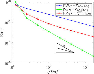
a

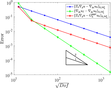
b

Figure 1: Counter example of superconvergence of the recovered gradient : (a) random $\mathcal{O}(h^{2})$ in the tangential direction; (b) random $\mathcal{O}(h^{2})$ in the normal direction.

2.2 Examples of $\mathcal{O}(h^{2})$ deviated manifolds

In this subsection, we present numerical examples which motivate further study in this paper. This illustrates why the concept of geometric supercloseness is needed. Especially, we show that barely with the condition (2.1), superconvergent rates of the recovered gradient may not be achieved as conjectured in [29]. Without loss of generality, we test the Laplace-Beltrami equation whose exact solution is $u=x_{1}x_{2}$ on the unit sphere. For the discretization, we use standard triangulation with nodes located on the sphere to get $\mathcal{M}_{h}^{*}$, and then add $\mathcal{O}(h^{2})$ random perturbation to the vertices of $\mathcal{M}_{h}^{*}$ in the tangential direction to get $\mathcal{M}_{h}^{1}$ and in the normal direction to get $\mathcal{M}_{h}^{2}$. To test the superconvergence property of the recovered gradient, we solve the Laplace-Beltrami equation on $\mathcal{M}_{h}^{i}$ ($i=1,2$) and the numerical results are summarized in Figure 1. We use PPPR scheme [11] for recovery which has been shown to have superconvergence under mildly structured mesh conditions with exact interpolation of the geometric. In the examples, we observe the optimal convergence for the finite element gradients and $\mathcal{O}(h^{2})$ supercloseness between the finite element gradient and the gradient of the interpolation of the exact solution on both meshes. That is

$$\left\|\nabla_{g_{h}}u_{I}-\nabla_{g_{h}}u_{h}\right\|_{0,\mathcal{M}_{h}^{i}}=\mathcal{O}(h^{2})\quad\text{ for }\;i=1,2,$$ (2.3)

where $u_{I}$ is the linear interpolation of exact solution and $u_{h}$ is the finite element solution. However, there is no superconvergence observed for the recovered gradient on those $\mathcal{O}(h^{2})$ deviated meshes. In [29], it has been proven that if the discretization is given by exact interpolation of the geometry, the supercloseness (2.3) leads to the superconvergence of the recovery of gradient under some shape conditions on the triangulation. The examples here send us the message that if the discretized geometry is $\mathcal{O}(h^{2})$ deviated, then (2.3) is not sufficient anymore to guarantee the superconvergence of the recovered gradient, instead, we need the superconvergence of differential structure of the manifolds. Motivated by this, we investigate next the geometric conditions for superconvergence in post-processing numerical solutions, which will also be used for designing optimal convergent numerical methods later in the paper.

3 Supercloseness of geometric approximation

In this section, we introduce the concept of geometric supercloseness between $\mathcal{M}_{h}$ and $\mathcal{M}_{h}^{*}$. This will entitle us the theoretical tool to show superconvergence of differential structure on deviated manifolds. We begin with some relevant definitions on triangular surface meshes. Based on the $\mathcal{O}(h^{2})$ parallelogram condition (e.g., [3, Definition 2.4]), we define the $\mathcal{O}(h^{2\sigma})$ irregular condition for the surface meshes .

Definition 3.1.

A triangular mesh $\mathcal{T}_{h}$ is said to satisfy the $\mathcal{O}(h^{2\sigma})$ irregular condition if there exist a partition $\mathcal{T}_{h,1}\bigcup\mathcal{T}_{h,2}$ of $\mathcal{T}_{h}$ and a positive constant $\sigma$ such that every two adjacent triangles in $\mathcal{T}_{h,1}$ form an $\mathcal{O}(h^{2})$ parallelogram and

$$\sum_{\tau_{h}\subset\mathcal{T}_{h,2}}\lvert\tau_{h}\rvert=\mathcal{O}(h^{2\sigma}).$$

To proceed, we introduce the concept of geometric supercloseness here.

Definition 3.2.

Let $\mathcal{M}_{h}^{*}$ and $\mathcal{M}_{h}$ be the exact interpolation and inexact approximation, respectively. We call $\mathcal{M}_{h}$ is geometrically superclose to $\mathcal{M}_{h}^{*}$ if the following requirements are satisfied:

• Let $g_{h}$ and $g_{h}^{*}$ be the metric tensors associated to $\mathcal{M}_{h}$ and $\mathcal{M}_{h}^{*}$ respectively, then

  $$\left\|g_{h}-g_{h}^{*}\right\|_{\infty}=\mathcal{O}(h^{2}).$$ (3.1)

• For every pair of patches on $\mathcal{M}_{h}$ and $\mathcal{M}_{h}^{*}$, there exist local parametrizations: $\mathbf{r}_{h}:\Omega\to\mathcal{M}_{h}$ and $\mathbf{r}_{h}^{*}:\Omega\to\mathcal{M}_{h}^{*}$, respectively, such that

  $$\left\|\partial\mathbf{r}_{h}-\partial\mathbf{r}_{h}^{*}\right\|_{\infty,\Omega}=\mathcal{O}(h^{2}).$$ (3.2)

In fact, the condition (3.2) implies (3.1), however, the reverse is not true. We show in the next section that (3.2) provides the ingredient for proving the superconvergence of recovered gradient on deviated discretization of manifolds.

To make the condition more concrete, we consider the following assumptions on the triangulations. We emphasis that the condition in Assumption 3.3 might not be the only case that leads to geometric supercloseness, however, it is quite practical to be fulfilled by the surface discretization algorithms using first order projections.

Assumption 3.3.

• The triangulation $\mathcal{M}_{h}$ is shape regular and quasi-uniform. Moreover, the $\mathcal{O}(h^{2\sigma})$ irregular condition holds for $\mathcal{M}_{h}$.

• $\mathcal{M}_{h}$ and $\mathcal{M}_{h}^{*}$ have the same amount of triangles and vertices, and every vertex pair of $\mathcal{M}_{h}$ and $\mathcal{M}^{*}_{h}$ satisfy the deviation condition that

  $$\lvert x_{h,i}-x_{h,i}^{*}\rvert=\mathcal{O}(h^{2})\text{ for all }\;i\in I_{h}.$$ (3.3)

• Let $\tau_{h,j}\in\mathcal{M}_{h}$ and $\tau_{h,j}^{*}\in\mathcal{M}_{h}^{*}$. If we parallel transfer each triangle pair $(\tau_{h,j},\tau^{*}_{h,j})$, to a common vertex, then the other two pairs of vertices (noted by $(\xi_{k_{j},h},\xi_{k_{j},h}^{*})$ after transformation) satisfy the distance condition that

  $$\lvert P_{\tau}(\xi_{k_{j},h}-\xi_{k_{j},h}^{*})\rvert=\mathcal{O}(h^{3})\;\text{ and }\;\lvert P_{n}(\xi_{k_{j},h}-\xi_{k_{j},h}^{*})\rvert=\mathcal{O}(h^{3}),\;\text{ for all }k_{j}\text{ and }j\in J_{h},$$ (3.4)

  where $P_{\tau}$, and $P_{n}$ are the normal and tangential projections to $\mathcal{M}_{h}^{*}$ respectively (alternatively, one can also consider both the projections to $\mathcal{M}_{h}$).

The first condition of Assumption 3.3 is quite standard, and it is crucial for proving superconvergence in the literature, e.g., [3, 30, 29]. However, in the manifold setting, this condition has been assumed on $\mathcal{M}_{h}^{*}$, which is the exact interpolation of $\mathcal{M}$. Note that condition (3.3) is exactly (2.1), however in addition, (3.4) is also required.

In the following, we show that Assumption 3.3 implies the geometric supercloseness for $\mathcal{M}_{h}$ to approximate $\mathcal{M}_{h}^{*}$. Before that, we need some auxiliary results first.

We consider $\tau_{1}$ and $\tau_{2}$ to be an triangle pair taken from $\mathcal{M}_{h}$ and $\mathcal{M}_{h}^{*}$. In the following analysis, we take one of triangle as a parametric domain, e.g., $\tau_{1}$, then there exist an linear map $\Gamma$ such that $\tau_{2}=\Gamma(\tau_{1})$. Note that $\Gamma:\mathbb{R}^{2}\to\mathbb{R}^{3}$, therefore $\partial\Gamma$ is a $3\times 2$ constant matrix. We denote $\operatorname{Id}=\left(\begin{matrix}1&0&0\\ 0&1&0\end{matrix}\right)^{\top}$.

Lemma 3.4.

Let $\tau_{1}$ and $\tau_{2}$ be shape regular triangle pair of diameter $h$ from $\mathcal{M}^{*}_{h}$ and $\mathcal{M}_{h}$ respectively, and the distance of each of their vertex pair satisfies condition (3.3), for $h\leq 1$ sufficiently small. In addition, we ask the first bounds in (3.4), i.e., the one with tangential projection. Then the following error bounds hold

$$\lvert l_{2,k}-l_{1,k}\rvert=\mathcal{O}(h^{3})\;\text{ and }\;\lvert l^{2}_{2,k}-l^{2}_{1,k}\rvert=\mathcal{O}(h^{4})\;\text{ for all }\;k=1,2,3,$$ (3.5)

where $\left\{l_{i,k}|{k=1,2,3}\right\}$ denotes the length of the three edges $\left\{e`_{i,k}|{k=1,2,3}\right\}$ of triangle $\tau_{i}$ for $i=1,2$.

Proof.

To see this we do parallel and vertical translation of $e_{2,k}$ to a common point with $e_{1,k}$, then for sufficiently small $h$ we have the estimate that

$$l_{2,k}\leq \sqrt{(l_{1,k}+c_{2,k}h^{3})^{2}+c_{1,k}h^{4}}$$

$$= l_{1,k}\sqrt{1+2c_{2,k}\frac{h^{3}}{l_{1,k}}+c_{2,k}^{2}\frac{h^{6}}{l^{2}_{1,k}}+c_{1,k}\frac{h^{4}}{l^{2}_{1,k}}}$$

$$\leq l_{1,k}\left(1+C(\frac{h^{3}}{l_{1,k}}+\frac{h^{6}}{l^{2}_{1,k}}+\frac{h^{4}}{l^{2}_{1,k}})\right).$$

Here both $c_{2,k}$ and $c_{1,k}$ are either positive or negative constants, which are corresponding to the tangential and normal errors respectively. Using the fact that $l_{1,k}\sim h$ for all $k=1,2,3$, then we get the first estimate in (3.5).

For the second estimate in (3.5), we only have to use $a^{2}-b^{2}=(a-b)(a+b)$, and taking into account that the edge lengths are of order $h$, then combining with the first estimate we have the conclusion. ∎

Lemma 3.5.

Under the same condition as Lemma 3.4, we have

$$\lvert\mathcal{A}(\tau_{2})-\mathcal{A}(\tau_{1})\rvert=\mathcal{O}(h^{4})\;\text{ and }\;\lvert\frac{\mathcal{A}(\tau_{2})}{\mathcal{A}(\tau_{1})}-1\rvert=\mathcal{O}(h^{2}),$$ (3.6)

where $\mathcal{A}$ is the area function.

Proof.

Taking the length of the edges of $\tau_{1}$ be $l_{1,k}$ for $k=1,2,3$, and then the length of the edges of $\tau_{2}$ will be $l_{2,k}=l_{1,k}+c_{k}h^{3}$ for some constant $c_{k}$ either being positive or negative due to (3.5). Now, we calculate the area of $\tau_{1}$ and $\tau_{2}$ using the edges info, i.e., Heron’s formula

$$\mathcal{A}(\tau_{1})=\sqrt{s_{1}\prod_{k}(s_{1}-l_{1,k})}\text{ and }\mathcal{A}(\tau_{2})=\sqrt{(s_{1}+d_{0}(\mathbf{c})h^{3})\prod_{k}(s_{1}-l_{1,k}+d_{k}(\mathbf{c})h^{3})},$$

where $s_{1}=\sum_{k}\frac{l_{1,k}}{2}$, and $\mathbf{c}=(c_{1},c_{2},c_{3})$. Thus we have

$$\lvert\frac{\mathcal{A}(\tau_{2})}{\mathcal{A}(\tau_{1})}-1\rvert= \lvert\sqrt{(1+d_{0}(\mathbf{c})\frac{h^{3}}{s_{1}})\prod_{k}(1+d_{k}(\mathbf{c})\frac{h^{3}}{s_{1}-l_{1,k}})}-1\rvert$$ (3.7)

$$= \lvert\sqrt{1+q_{0}(\mathbf{c})h^{2}}\prod_{k}\sqrt{1+q_{k}(\mathbf{c})h^{2}}-1\rvert$$

$$\leq \lvert(1+Cq_{0}(\mathbf{c})h^{2})\prod_{k}(1+Cq_{k}(\mathbf{c})h^{2})-1\rvert$$

$$\leq C(\mathbf{q})h^{2}$$

for some constants $\mathbf{q}=(q_{0},q_{1},q_{2},q_{3})$ depending on $\mathbf{c}$. Thus we have constant $C$ depends on $\mathbf{c}$. The first estimate in (3.6) is obvious since $\mathcal{A}(\tau_{1})$ is also of order $h^{2}$. Multiply with $\mathcal{A}(\tau_{1})$ on both side of (3.7) gives the estimate. ∎

Proposition 3.6.

Assume the same condition as Lemma 3.4. Let $\Gamma:\tau_{1}\to\tau_{2}$ be the linear transformation, and let $g_{\Gamma}:=(\partial\Gamma)^{\top}\partial\Gamma$. Then we have following relations:

• The determinate of $g_{\Gamma}$ satisfies

  $$\lvert\sqrt{\det{g_{\Gamma}}}-1\rvert=\mathcal{O}(h^{2}).$$ (3.8)

• The Jacobian $\partial\Gamma$ and the metric $g_{\Gamma}$ have the following estimate

  $$\left\|\partial\Gamma-\operatorname{Id}\right\|_{\infty}=\mathcal{O}(h)\;\text{ and }\;\left\|g_{\Gamma}-\operatorname{I}\right\|_{\infty}=\mathcal{O}(h^{2}),$$ (3.9)

  respectively, where $\operatorname{I}=\operatorname{Id}^{\top}\operatorname{Id}$ is the $2\times 2$ identity matrix.

• Let the second condition in (3.4) hold additionally, i.e., the one with normal projection. Then we have an improved error estimate for the Jacobian matrix

  $$\left\|\partial\Gamma-\operatorname{Id}\right\|_{\infty}=\mathcal{O}(h^{2}).$$ (3.10)

Proof.

(i). To show (3.8), notice $\mathcal{A}(\tau_{2})=\sqrt{\det{g_{\Gamma}}}\mathcal{A}(\tau_{1})$. Applying the estimate (3.6) in Lemma 3.5 we have

$$\lvert\sqrt{\det{g_{\Gamma}}}-1\rvert=\lvert\frac{\mathcal{A}(\tau_{2})}{\mathcal{A}(\tau_{1})}-1\rvert=\mathcal{O}(h^{2})$$

which then leads to the first estimate in (3.8).

(ii). For the first one in (3.9), we notice that $g=(\partial\Gamma)^{\top}\partial\Gamma$. Since we choose $\tau_{1}$ to be the parametric domain of $\tau_{2}$, then $\tau_{2}=\partial\Gamma\tau_{1}+x_{0}$. Now we transfer the two triangles to a common vertex, and change the Cartesian coordinate to let the common vertex be at the origin. Let the position of two other vertices of $\tau_{1}$ in the new coordinate be $\xi_{1}=(\xi_{1,1},\xi_{1,2},0)$ and $\xi_{2}=(\xi_{2,1},\xi_{2,2},0)$, and the corresponding vertices of $\tau_{2}$ be $\psi_{1}=(\psi_{1,1},\psi_{1,2},\psi_{1,3})$ and $\psi_{2}=(\psi_{2,1},\psi_{2,2},\psi_{2,3})$. Then we have $\psi_{k}=\Gamma\xi_{k}$ for $k=1,2$. Then we have

$$\partial\Gamma=\left(\begin{matrix}\psi_{1,1}&\psi_{2,1}\\ \psi_{1,2}&\psi_{2,2}\\ \psi_{1,3}&\psi_{2,3}\\ \end{matrix}\right)\left(\begin{matrix}\xi_{1,1}&\xi_{2,1}\\ \xi_{1,2}&\xi_{2,2}\\ \end{matrix}\right)^{-1}$$

Then we have that

$$\partial\Gamma-\operatorname{Id}=\left(\left(\begin{matrix}\psi_{1,1}&\psi_{2,1}\\ \psi_{1,2}&\psi_{2,2}\\ \psi_{1,3}&\psi_{2,3}\\ \end{matrix}\right)-\left(\begin{matrix}\xi_{1,1}&\xi_{2,1}\\ \xi_{1,2}&\xi_{2,2}\\ 0&0\end{matrix}\right)\right)\left(\begin{matrix}\xi_{1,1}&\xi_{2,1}\\ \xi_{1,2}&\xi_{2,2}\\ \end{matrix}\right)^{-1}.$$ (3.11)

Because $(\xi_{i,j})_{i,j\in\left\{1,2\right\}}$ are all of order $h$, and $(\lvert\xi_{1,1}\xi_{2,2}-\xi_{2,1}\xi_{1,2}\rvert)/2$ equals the area of $\tau_{1}$ therefore of order $h^{2}$, then we can conclude that

$$\left(\begin{matrix}\xi_{1,1}&\xi_{2,1}\\ \xi_{1,2}&\xi_{2,2}\\ \end{matrix}\right)^{-1}=\left(\begin{matrix}\xi_{2,2}&-\xi_{1,2}\\ -\xi_{2,1}&\xi_{1,1}\\ \end{matrix}\right)(\lvert\xi_{1,1}\xi_{2,2}-\xi_{2,1}\xi_{1,2}\rvert)^{-1}=M/h$$ (3.12)

where $M$ is some constant matrix independent of $h$.

Recall that $\psi_{1}$, $\psi_{2}$ are vertices of $\tau_{2}$, and $\xi_{1}$, $\xi_{2}$ are vertices of $\tau_{1}$ in the new coordinates. Due to our assumption (3.3), we have difference of the tangential part

$$\lvert\psi_{i,j}-\xi_{i,j}\rvert=\mathcal{O}(h^{3})\;\text{ for }\quad i=1,2,\;\;j=1,2$$ (3.13)

and the normal part

$$\lvert\psi_{i,3}\rvert=\mathcal{O}(h^{2})\text{ for }i=1,2.$$ (3.14)

Going back to (3.11) with also the estimate in (3.12), we have then

$$\left\|\partial\Gamma-\operatorname{Id}\right\|_{\infty}=\mathcal{O}(h).$$

Now we show the second one in (3.9). Since $g_{\Gamma}=(\partial\Gamma)^{\top}\partial\Gamma$. Thus

$$g_{\Gamma}-\operatorname{I}=\left(\begin{matrix}\xi_{1,1}&\xi_{1,2}\\ \xi_{2,1}&\xi_{2,2}\\ \end{matrix}\right)^{-1}\left(\left(\begin{matrix}\psi_{1}\cdot\psi_{1}&\psi_{1}\cdot\psi_{2}\\ \psi_{2}\cdot\psi_{1}&\psi_{2}\cdot\psi_{2}\end{matrix}\right)-\left(\begin{matrix}\xi_{1}\cdot\xi_{1}&\xi_{1}\cdot\xi_{2}\\ \xi_{2}\cdot\xi_{1}&\xi_{2}\cdot\xi_{2}\end{matrix}\right)\right)\left(\begin{matrix}\xi_{1,1}&\xi_{2,1}\\ \xi_{1,2}&\xi_{2,2}\\ \end{matrix}\right)^{-1}.$$ (3.15)

Thus we have $\psi_{i}\cdot\psi_{i}$ for $i=1,2$ been the length square of the edges of $\tau_{2}$ and as well as $\xi_{i}\cdot\xi_{i}$ for $\tau_{1}$. Thus from Lemma 3.4, we have

$$\lvert\psi_{i}\cdot\psi_{i}-\xi_{i}\cdot\xi_{i}\rvert=\mathcal{O}(h^{4}),\text{ for }i=1,2$$

On the other hand, $\psi_{i}\cdot\psi_{j}$ for $i\neq j$ returns $2\mathcal{A}(\tau_{2})$, and $\xi_{i}\cdot\xi_{j}$ for $i\neq j$ gives $2\mathcal{A}(\tau_{1})$. Thus using Lemma 3.5 we have

$$\lvert\psi_{i}\cdot\psi_{j}-\xi_{i}\cdot\xi_{j}\rvert=2\lvert\mathcal{A}(\tau_{2})-\mathcal{A}(\tau_{1})\rvert=\mathcal{O}(h^{4})\text{ for }i\neq j.$$

Taking into account again (3.12) and return to (3.15), we have

$$\left\|g_{\Gamma}-\operatorname{I}\right\|=\mathcal{O}(h^{2}).$$

(iii). We go back to the formula in (3.11). Note that the additional condition in (3.4) of normal direction error increases the order of $\lvert\psi_{i,3}\rvert$ in (3.14). That is

$$\lvert\psi_{i,3}\rvert=\mathcal{O}(h^{3})\quad\text{ for }i=1,2,$$

which is then of the same order as $\lvert\psi_{i,j}-\xi_{i,j}\rvert$ for $i=1,2$ $j=1,2$ in (3.13). Thus we conclude the statement by comparing the proof of the first estimate in (3.9). ∎

We emphasize here that with only assumption (3.3) and the tangential condition in (3.4), it is already able to prove the metric condition (3.8). However, it is not sufficient to conclude the Jacobian condition (3.10), which is needed for the geometric supercloseness.

With the above preparation, we are ready to show that Assumption 3.3 gives us supercloseness of the geometric approximation.

Proposition 3.7.

Let $\mathcal{M}_{h}$ and $\mathcal{M}^{*}_{h}$ satisfy Assumption 3.3, then we have

• The triangulation $\mathcal{M}^{*}_{h}$ is also shape regular and quasi-uniform, and the $\mathcal{O}(h^{2\sigma})$ irregular condition is fulfilled for $\mathcal{M}^{*}_{h}$.

• The local piece-wise linear parametrization functions, $\mathbf{r}_{h,i}$ and $\mathbf{r}^{*}_{h,i}$, satisfy

  $$\left\|\partial\mathbf{r}_{h,i}-\partial\mathbf{r}^{*}_{h,i}\right\|_{0,\Omega_{i}}=\sqrt{\mathcal{A}(\mathcal{M}^{*}_{h,i})}\mathcal{O}(h^{2}),\;\;\text{ for all }\;i\in I_{h}.$$ (3.16)

  Here $\mathcal{A}$ is the area functional, and $\mathcal{M}^{*}_{h,i}\subset\mathcal{M}^{*}_{h}$ is the patch corresponding to the parameter domain $\Omega_{i}$. To simplify the discussion, we choose the same $\Omega_{i}$ for both $\mathcal{M}_{h,i}$ and $\mathcal{M}_{h,i}^{*}$, which is obtained as Algorithm 1.

Proof.

The first assertion holds because the triangles of $\mathcal{M}_{h}$ are shape regular and quasi-uniform, and they satisfy the $\mathcal{O}(h^{2\sigma})$ irregular condition above. The definition of shape regular and quasi-uniform can be found in many textbooks of finite element methods [5, 7]. Using the triangle inequality, we get the conclusion.

Now we prove the second assertion. Let $\Omega_{i}$ be the parameter domain for patches selected around the vertex $x_{h,i}$. Denote the local index-set associated to vertices of the selected patch around $x_{h,i}$ to be $J_{i}$. We notice that both $\mathbf{r}_{h,i}$ and $\mathbf{r}^{*}_{h,i}$ are piecewise linear functions defined on $\Omega_{i}$. Let $\Omega_{i,j}$ be the common parameter domain for the corresponding triangle pairs $\tau_{h,j}$ and $\tau^{*}_{h,j}$ for the index $j\in J_{i}$. Then $\mathbf{r}_{h,i}$ and $\mathbf{r}^{*}_{h,i}$ are linear functions on each of the regions $\Omega_{i,j}$ for every $j\in J_{i}$. Note that due to the construction of $\Omega_{i}$ (see Algorithm 1), the change of coordinates from $\Omega_{i,j}$ to $\tau_{h,j}$ or $\tau^{*}_{h,j}$ is done by linear transformation.

Since the Jacobian $\partial\mathbf{r}_{h,i}$ and $\partial\mathbf{r}^{*}_{h,i}$ are constant functions, we have

$$\left\|\partial\mathbf{r}_{h,i}-\partial\mathbf{r}^{*}_{h,i}\right\|_{0,\Omega_{i,j}} \leq(\sup_{i,j}{\sqrt{\frac{\mathcal{A}(\Omega_{i,j})}{\mathcal{A}(\tau^{*}_{h,j})}}})\left\|R_{i,j}\right\|\left\|\partial\Gamma_{j}-\operatorname{Id}\right\|_{0,\tau^{*}_{h,j}}$$

$$\leq\left\|\partial\Gamma_{j}-\operatorname{Id}\right\|_{0,\tau^{*}_{h,j}}.$$

Here $R_{i,j}$ is a $3\times 3$ matrix to change coordinates from $\tau^{*}_{h,j}$ to $\Omega_{i,j}$, which is a projection matrix, and thus $\left\|R_{i,j}\right\|=1$; $\Gamma_{j}$ is the geometric mapping from $\tau^{*}_{h,j}$ to $\tau_{h,j}$, which can be obtained from $\mathbf{r}_{h,i}$ by changing the local coordinates from $\Omega_{i,j}$ to $\tau^{*}_{h,j}$, while the mapping $\mathbf{r}^{*}_{h,i}$ becomes identity after this change of coordinates. Due to the shape regularity of $\mathcal{M}_{h}$ and $\mathcal{M}^{*}_{h}$, and $\mathcal{M}$ has bounded curvature, thus all the elements of $\left\{\sqrt{\frac{\mathcal{A}(\Omega_{i,j})}{\mathcal{A}(\tau^{*}_{h,j})}}\right\}_{i\in I_{h},j\in J_{h}}$ are uniformly bounded from below and from above on all the parametric domain $\left\{\Omega_{i}\right\}_{i\in I_{h}}$ and the triangles $\left\{\tau^{*}_{h,j}\right\}_{j\in J_{h}}$. Typically, we have $\sup_{i,j}\sqrt{\frac{\mathcal{A}(\Omega_{i,j})}{\mathcal{A}(\tau^{*}_{h,j})}}\leq 1$ due to the fact that $\Omega_{i,j}$ is the projection of $\tau^{*}_{h,j}$ onto $\Omega_{i}$.

Applying the result from Proposition 3.6, we have

$$\left\|\partial\mathbf{r}_{h,i}-\partial\mathbf{r}^{*}_{h,i}\right\|_{0,\Omega_{i,j}}\leq\left\|\partial\Gamma_{j}-\operatorname{Id}\right\|_{0,\tau^{*}_{h,j}}\leq C\sqrt{\mathcal{A}(\tau_{h,j}^{*})}h^{2}.$$

Summing up over $j\in J_{i}$, we arrive at the following inequality

$$\left\|\partial\mathbf{r}_{h,i}-\partial\mathbf{r}^{*}_{h,i}\right\|_{0,\Omega_{i,j}}=\mathcal{O}(h^{4})\sum_{j\in J_{i}}\mathcal{A}(\tau_{h,j}^{*}).$$

Taking square root on both sides gives the conclusion of the second assertion. ∎

The relation in (3.16) tells in fact some regularity on the approximations of $\mathcal{M}_{h}$ to $\mathcal{M}$. It is similar to the supercloseness property for the gradient of the finite element solutions to the gradient of the interpolation of the exact solutions [3, 30]. This would then leads to the superconvergence of the differential structure on deviated manifolds.

In what follows, we present two concrete case study where superconvergence of the differential structure of manifolds are crucial. The first application is on post-processing numerical solutions, e.g., finite element solution of elliptic partial differential equations on discretized manifolds, and the second is on an a priori optimal convergence analysis for problems whose solutions are tangential vector fields on manifolds.

4 Case study I: Superconvergence of gradient recovery on deviated manifolds

4.1 Isoparametric gradient recovery schemes on manifolds

Here, we generalize the idea of parametric polynomial preserving recovery proposed in [11] to have a general family of recovery methods in manifolds setting. More precisely, the algorithm framework generalizes the methods introduced in [29], which ask for exact geometry-prior, to the case without exact geometry-prior. To do this, we rely on the intrinsic definition of gradient operator on manifolds. Given a local parametric patch, and $\mathbf{r}:\Omega\to\mathcal{M}$ the parametrization function of this patch, define $\bar{u}:=u\circ\mathbf{r}$. Then we have

$$(\nabla_{g}u)\circ\mathbf{r}=\nabla\bar{u}(g\circ\mathbf{r})^{-1}\partial\mathbf{r}=\nabla\bar{u}(\partial\mathbf{r})^{\dagger}\quad\text{ on }\Omega.$$ (4.1)

Here $(\partial\mathbf{r})^{\dagger}$ is the pseudo-inverse of the Jacobian $\partial\mathbf{r}$. For a small digest of differential operator on manifolds, we refer to the appendix of [12] and also the background part in [11]. One may refer to the textbooks, e.g., [10] for more comprehensive introduction on differential geometry. Inspired from (4.1), we try to recover the gradient on manifolds using a two-level strategy. That is to recover the Jacobian $\partial\mathbf{r}$ and also $\nabla\bar{u}$ iso-parametrically on every local patch. We call the new methods as isoparametric gradient recovery schemes. They ask for neither the exact vertices nor the precise tangent spaces. In particular the PPPR method which was introduced in [11] can also be included into this framework.

Algorithm 1 Isoparametric geometric recovery and gradient recovery schemes

Input: Discretized triangular surface $\mathcal{M}_{h}$ with vertices set $(x_{h,i})_{i\in I_{h}}$ and the data (FEM solutions) $(u_{h,i})_{i\in I_{h}}$. Then we suggest a two stages recovery steps for all $i\in I_{h}$.

$\bullet$ Geometric recovery:

• At every $x_{h,i}$, select a local patch $\mathcal{M}_{h,i}\in\mathcal{M}_{h}$ around $x_{h,i}$ with sufficient vertices. Compute the unit normal vectors of every triangle faces in $\mathcal{M}_{h,i}$. Compute the simple (weighted) average of the unit normal vectors, and normalize it to be $\phi^{3}_{i}$. Take the orthogonal space to $\phi^{3}_{i}$ to be the parametric domain $\Omega_{i}$. Shift $x_{h,i}$ to be the origin of $\Omega_{i}$, and choose $(\phi^{1}_{i},\phi^{2}_{i})$ the orthonormal basis of $\Omega_{i}$.

• Project all selected vertices of $\mathcal{M}_{h,i}$ around $x_{h,i}$ onto the parametric domain $\Omega_{i}$ from Step $(1)$, and record the new coordinates as $\zeta_{i_{j}}$.

• Use a planar recovery scheme $R^{k}_{h}$ to recover the surface Jacobian with respect to $\Omega_{i}$. Typically, this is considered every surface patch as local graph of some function $s$, that is $\mathbf{r}_{i}=(\Omega_{i},s_{i}(\Omega_{i}))$. Then the recovered Jacobian at the selected patch is $J_{r,i}=(\operatorname{I},R^{k}_{h}s_{i,j})^{\top}$, where $\operatorname{I}$ is the identity matrix of the dimension $\Omega_{i}$.

$\bullet$ Function gradient recovery:

• Let $(\bar{u}_{h,j})_{j\in I_{i}}$ be the values of $(u_{h,j})_{j\in I_{i}}$ associated to vertices of $\mathcal{M}_{h,i}$ isoparametrically defined on the parameter domain $\Omega_{i}$. Then using the same planar recovery scheme $R^{k}_{h}$ to recover gradient from $(\bar{u}_{h,j})_{j\in I_{i}}$ with respect to parameter domain $\Omega_{i}$.

• In the spirit of (4.1), use the results from Step $(3)$ and Step $(4)$ to get the recovered surface gradient at $x_{h,i}$:

  $$G^{k}_{h}u_{h,i}=R^{k}_{h}\bar{u}_{h,i}(J_{r,i})^{\dagger}(\phi^{1}_{i},\phi^{2}_{i},\phi^{3}_{i}),$$ (4.2)

  where $(J_{r,i})^{\dagger}=(J_{r,i}J_{r,i}^{\top})^{-1}J_{r,i}$. The orthonormal basis $\left\{\phi^{1}_{i},\phi^{2}_{i},\phi^{3}_{i}\right\}$ is multiplied to unify the coordinates from local ones to a global one in the ambient Euclidean space.

Output: The recovered gradient at selected nodes $\left\{G^{k}_{h}u_{h,i}\right\}_{i\in I_{h}}$. For $x$ being not a vertex of triangles, we use linear finite element basis to interpolate the values $\left\{G_{h}u_{h,i}\right\}_{i\in I_{h}}$ at vertices of each triangle.

Algorithm 1 in fact describes a family of recovery methods. The generality should also cover higher dimensional problems, but for simplicity, we focus on $2$-dimensional case only.

Note that we do not specify the concrete recovery methods in Step $(3)$ and Step $(4)$. Actually, almost all the local recovery methods for functions in the Euclidean domain can be applied. This would include many of the methods which have been discussed in [29]. Though the preferred candidates will be $ZZ$-scheme and PPR. The latter gives then the PPPR method proposed in [11]. In view of (4.2), one can see that it is an approximation of (4.1) at every nodes: $R^{k}_{h}\bar{u}_{h,i}$ recovers $\nabla\bar{u}$, and $(J_{r,i})^{\dagger}(\phi^{1}_{i},\phi^{2}_{i},\phi^{3}_{i}),$ recovers $(\partial\mathbf{r})^{\dagger}$. Moreover, it gives the intuition that why the resulting in (3.16) is required in order to match the superconvergence of the function gradient recovery and the superconvergence of the geometric structures, simultaneously. In the next section, we will show the superconvergence property of the recovery scheme.

4.2 Superconvergence analysis on deviated geometry

Even though we have shown a general algorithmic framework, which can cover several different methods under the same umbrella, we will focus on parametric polynomial preserving recovery scheme for the theoretical analysis. It asks for fewer requirements on the meshes in comparison with several other methods, e.g., for simple (weighted) average, or generalized ZZ-scheme, which require an additional $\mathcal{O}(h^{2})$-symmetric condition. However, the general idea of the proof is extendable to the other methods as well.

We take the following Laplace-Beltrami equation as our model problem to conduct the analysis:

$$-\Delta_{g}u=f\quad\text{ where }\;\int_{\mathcal{M}}f\;dvol=0,$$ (4.3)

The weak formulation of equation (4.3) is given as follows: Find $u\in H^{1}(\mathcal{M})$ with $\int_{\mathcal{M}}u\;dvol=0$ such that

$$\int_{\mathcal{M}}\nabla_{g}u\cdot\nabla_{g}v\;dvol=\int_{\mathcal{M}}fv\;dvol,\quad\forall v\in H^{1}(\mathcal{M}).$$ (4.4)

The regularity of the solution has been proved in [2, Chapter 4]. In the surface finite element method, the surface $\mathcal{M}$ is approximated by the triangulation $\mathcal{M}_{h}$ which satisfy Assumption 3.3, and the solution is simulated in the continuous piecewise linear function space $\mathcal{V}_{h}$ defined over $\mathcal{M}_{h}$, i.e.

$$\int_{\mathcal{M}_{h}}\nabla_{g_{h}}u_{h}\cdot\nabla_{g_{h}}v_{h}\;dvol_{h}=\int_{\mathcal{M}_{h}}f_{h}v_{h}\;dvol_{h},\quad\forall v_{h}\in\mathcal{V}_{h}(\mathcal{M}_{h}).$$ (4.5)

We first show that there exists an underline smooth manifold denoted by $\widetilde{\mathcal{M}}_{h}$ so that $\mathcal{M}_{h}$ can be thought as an interpolation of it. This intermediate manifold is not needed practically in the algorithm, but it is helpful for our error analysis.

Proposition 4.1.

Let $\mathcal{M}$ be the precise manifold, and $\mathcal{M}_{h}$ and $\mathcal{M}_{h}^{*}$ satisfy the assumption 3.3. Then the following statements hold true:

• There exists a $C^{3}$ smooth manifold $\widetilde{\mathcal{M}}_{h}$, so that $\mathcal{M}_{h}$ is a linear interpolation of $\widetilde{\mathcal{M}}_{h}$ at the vertices. Moreover, the Jacobian of the local geometric mapping at each vertex equals to the recovered geometry Jacobian using gradient recovery method.

• Let $\mathbf{r}_{\tau_{h,j}}$ and $\tilde{\mathbf{r}}_{\tau_{h,j}}$ be the parametrization of the curved triangular surfaces $\tau_{j}\subset\mathcal{M}$ and $\tilde{\tau}_{h,j}\subset\widetilde{\mathcal{M}}_{h}$ from the triangle $\tau_{h,j}$, respectively. Then there is the estimate

  $$\left\|\partial\tilde{\mathbf{r}}_{\tau_{h,j}}-\partial\mathbf{r}_{\tau_{h,j}}\right\|_{\infty,\tau_{h,j}}\leq Ch^{2}$$ (4.6)

  where $C$ is a constant independent of $h$.

• Let $v:\mathcal{M}\to\mathbb{R}$ be functions in $W^{k,p}(\mathcal{M})$, and $\tilde{v}_{h}$ be the pullback of $v$ to $\widetilde{\mathcal{M}}_{h}$, then we have

  $$C_{1}\left\|\tilde{v}_{h}\right\|_{W^{k,p}(\widetilde{\mathcal{M}}_{h})}\leq\left\|v\right\|_{W^{k,p}(\mathcal{M})}\leq C_{2}\left\|\tilde{v}_{h}\right\|_{W^{k,p}(\widetilde{\mathcal{M}}_{h})},$$ (4.7)

  for some constants $0<C_{1}\leq C_{2}$.

Proof.

$(i)$ For the first statement, we design the following algorithm to construct the smooth manifold $\widetilde{\mathcal{M}}_{h}$, though it is not needed in practice but only for theoretically judgment.

• At each vertex $x_{i}$ of $\mathcal{M}_{h}$, we use PPR algorithm [31] to recover the local geometry as a graph of a scalar function $s_{i}$ for $i\in I_{h}$ on $\Omega_{i}$, and calculate its gradient vector under the coordinates $\Omega_{i}$.

• For each triangle $\tau_{h,j}$ with $j\in J_{h}$, we build a local coordinate system, take the barycenter of $\tau_{h,j}$ as the origin, and transfer the recovered functions $\left\{s_{i}\right\}$ associated to $\tau_{h,j}$ from $\Omega_{i}$ to the new local coordinate, individually. Also, the recovered gradient vector for $s_{i}$ at the vertex $x_{i}$ is represented with respect to the new coordinates on $\tau_{h,j}$.

• We use a $3^{rd}$ order polynomial to fit the function and gradient values over $\tau_{h,j}$. The data are function values at the $3$ vertices (in fact with function value $0$), and the represented gradient values of $s_{i}$ at each vertex $x_{i}$ which contribute $6$ directional derivative values on the $3$ edges of $\tau_{h,j}$ since one vertex shared by two edges of $\tau_{h,j}$. This gives $9$ linearly independent equations in total.

• We put another constraint that the local polynomial value at the barycenter of every triangle $\tau_{h,j}$ matches the function value whose graph is the patch $\tau_{j}$ at the normal cross with the barycenter of $\tau^{*}_{h,j}$.

• We have now $10$ linear independent equations in total on each triangle $\tau_{h,j}$, thus a $3^{rd}$ order local polynomial is uniquely determined.

• Going through all the indexes $j\in J_{h}$ with the described algorithm. This gives us an element-wise $3^{rd}$ order polynomial patches which we denote by $\widetilde{\mathcal{M}}_{h}$. Note that on every edge of the triangles, it is a one dimensional $3^{rd}$ order polynomial function which is uniquely determined by the vertices and the directional derivatives conditions. Since polynomials at neighbored triangle edges are invariant under affine coordinate transformation, the local polynomials matches each other at every edge of neighbored triangles. Therefore $\widetilde{\mathcal{M}}_{h}$ is continuous at every edge and thus closed.

So far the construction of $\widetilde{\mathcal{M}}_{h}$ shows that it is a $C^{1}$ manifold. Now we apply Whitney’s approximation theorem (see, e.g., [21, Theorem 2.9]) which states that for every $C^{1}$ manifold, there exists compatible $C^{k}$ (for any $k\in[1,\infty]$) smoothness manifolds which can approximate the $C^{1}$ manifold arbitrarily close. We still use the notation $\widetilde{\mathcal{M}}_{h}$ for the smoothed version of $\widetilde{\mathcal{M}}_{h}$.

$(ii)$ For the second statement, we notice the following relation:

$$\left\|\partial\mathbf{r}_{\tau_{h,j}}-\partial\tilde{\mathbf{r}}_{\tau_{h,j}}\right\|_{\infty,\tau_{h,j}}\leq \left\|\partial\mathbf{r}_{\tau_{h,j}}-\bar{G}_{h}\Gamma^{*}_{j}\right\|_{\infty,\tau_{h,j}}+\left\|\bar{G}_{h}\Gamma^{*}_{j}-\bar{G}_{h}\Gamma_{j}\right\|_{\infty,\tau_{h,j}}$$ (4.8)

$$+\left\|\bar{G}_{h}\Gamma_{j}-\partial\tilde{\mathbf{r}}_{\tau_{h,j}}\right\|_{\infty,\tau_{h,j}}.$$

Here we take $\tau_{h,j}$ the parameter domain for both $\mathbf{r}_{\tau_{h,j}}$ and $\tilde{\mathbf{r}}_{\tau_{h,j}}$. $\Gamma^{*}_{j}$ and $\Gamma_{j}$ are the local geometric transformations which are obtained from the linear interpolations of the geometric mapping $\mathbf{r}_{\tau_{h,j}}$ and $\tilde{\mathbf{r}}_{\tau_{h,j}}$ at the vertices of $\tau_{h,j}$, respectively. Note that here we always chose $\tau_{h,j}$ to be the parameter domain, therefore $\Gamma_{j}\equiv\operatorname{Id}$ for all $j\in J_{h}$. $\bar{G}_{h}$ is the local PPR gradient recovery operator.

The first and the third terms on the right-hand side of (4.8) can be estimated using polynomial preserving properties of $\bar{G}_{h}$ and the smoothness of the functions $\mathbf{r}_{\tau_{h,j}}$ and $\tilde{\mathbf{r}}_{\tau_{h,j}}$, which gives

$$\left\|\partial\mathbf{r}_{\tau_{h,j}}-\bar{G}_{h}\Gamma^{*}_{j}\right\|_{\infty,\tau_{h,j}}\leq c_{1}\left\|\mathbf{r}_{\tau_{h,j}}\right\|_{3,\tau_{h,j}}h^{2},\quad\left\|\bar{G}_{h}\Gamma_{j}-\partial\tilde{\mathbf{r}}_{\tau_{h,j}}\right\|_{\infty,\tau_{h,j}}\leq c_{2}\left\|\tilde{\mathbf{r}}_{\tau_{h,j}}\right\|_{3,\tau_{h,j}}h^{2}.$$ (4.9)

Here $\bar{G}_{h}$ is realized using the linear interpolation of the recovered gradients of $s_{i}$ at the every vertices of $\tau_{h,j}$ transformed under the local coordinates on $\tau_{h,j}$. The second term on the right-hand side of (4.8) can be estimated from Lemma 4.2 and the boundedness result of the planar recovery operator $\bar{G}_{h}$ [23, Theorem 3.2]:

$$\left\|\bar{G}_{h}\Gamma^{*}_{j}-\bar{G}_{h}\Gamma_{j}\right\|_{\infty,\tau_{h,j}}\leq C\left\|\partial\Gamma^{*}_{j}-\partial\Gamma_{j}\right\|_{\infty,\tau_{h,j}}\leq c_{3}h^{2}.$$ (4.10)

Since $\left\|\mathbf{r}_{\tau_{h,j}}\right\|_{3,\tau_{h,j}}$ and $\left\|\tilde{\mathbf{r}}_{\tau_{h,j}}\right\|_{3,\tau_{h,j}}$ both are uniformly bounded, combining (4.9) and (4.10) and returning to (4.8) give the estimate

$$\left\|\partial\mathbf{r}_{\tau_{h,j}}-\partial\tilde{\mathbf{r}}_{\tau_{h,j}}\right\|_{\infty,\tau_{h,j}}=\mathcal{O}(h^{2}).$$

$(iii)$ For the equivalence (4.7) we can use the results in [8, page 811], which is able to show the equivalence on each triangle pairs of $\mathcal{M}_{h}$ and $\widetilde{\mathcal{M}}_{h}$, that is

$$c_{j,1}\left\|\tilde{v}_{h}\right\|_{W^{k,p}(\widetilde{\tau}_{h,j})}\leq\left\|v_{h}\right\|_{W^{k,p}(\tau_{h,j})}\leq c_{j,2}\left\|\tilde{v}_{h}\right\|_{W^{k,p}(\widetilde{\tau}_{h,j})},$$

for some constants $\left\{c_{j,1}\right\}_{j\in J_{h}}>0$ and $\left\{c_{j,2}\right\}_{j\in J_{h}}>0$. The equivalence for functions defined on triangle pairs of $\tau_{j}$ and $\tau_{h,j}$ is similarly shown. Then we arrive the following

$$\tilde{c}_{j,1}\left\|\tilde{v}_{h}\right\|_{W^{k,p}(\widetilde{\tau}_{h,j})}\leq\left\|v\right\|_{W^{k,p}(\tau_{j})}\leq\tilde{c}_{j,2}\left\|\tilde{v}_{h}\right\|_{W^{k,p}(\widetilde{\tau}_{h,j})}.$$

with constants $\left\{\tilde{c}_{j,1}\right\}_{j\in J_{h}}>0$ and $\left\{\tilde{c}_{j,2}\right\}_{j\in J_{h}}>0$. Since $\mathcal{M}_{h}\to\mathcal{M}$ as $h\to 0$, we have $\widetilde{\mathcal{M}}_{h}\to\mathcal{M}$ as well. This tells that $\tilde{c}_{j,1},\;\tilde{c}_{j,2}\to 1$ as $h\to 0$, which indicates that the constants $\left\{\tilde{c}_{j,1}\right\}_{j\in J_{h}}$ and $\left\{\tilde{c}_{j,2}\right\}_{j\in J_{h}}$ are uniformly bounded. Then we derive the equivalence in (4.7). ∎

In order to prove the superconvergence in the case when the vertices of $\mathcal{M}_{h}$ are not located exactly on $\mathcal{M}$, but in a $h^{2}$-neighborhood around it, we use the following estimate.

Lemma 4.2.

Let assume the Assumption 3.3 hold, and let $\widetilde{\mathcal{M}}_{h}$ be constructed from Proposition 4.1. Let $v\in W^{3,\infty}(\mathcal{M})$, and let $\tilde{v}_{h}:=\tilde{T}_{h}v$ be pullback of $v$ from $\mathcal{M}$ to $\widetilde{\mathcal{M}}_{h}$: $\tilde{v}_{h}(\tilde{\mathbf{r}}_{h,i}(\zeta))=v(\mathbf{r}_{i}(\zeta))$ for every $\zeta\in\Omega_{i}$ and all $i\in I_{h}$, where $\tilde{\mathbf{r}}_{h,i}:\Omega_{i}\to\widetilde{\mathcal{M}}_{h,i}$ and $\mathbf{r}_{i}:\Omega_{i}\to\mathcal{M}_{i}$. Then the following estimate holds:

$$\left\|\nabla_{g}v-(\tilde{T}_{h})^{-1}\nabla_{\tilde{g}_{h}}\tilde{v}_{h}\right\|_{0,\mathcal{M}}\lesssim h^{2}\left\|\nabla_{g}v\right\|_{0,\mathcal{M}}.$$ (4.11)

Proof.

Recall (4.1) for the definition of gradient in the local parametric domain, particularly, we take the local parametric domain to be $\tau_{h,j}$. Then we have for every $j\in J_{h}$ the following estimates

$$\left\|\nabla_{g}v-(\tilde{T}_{h})^{-1}\nabla_{\tilde{g}_{h}}\tilde{v}_{h}\right\|^{2}_{0,\tau_{j}}=\int_{\tau_{h,j}}\lvert\nabla\bar{v}\left((\partial\mathbf{r}_{\tau_{h,j}})^{\dagger}-(\partial\tilde{\mathbf{r}}_{\tau_{h,j}})^{\dagger}\right)\rvert^{2}\sqrt{\det(\partial\mathbf{r}_{\tau_{h,j}}(\partial\mathbf{r}_{\tau_{h,j}})^{\top})}$$ (4.12)

$$\leq \left\|\operatorname{I}-\partial\mathbf{r}_{\tau_{h,j}}(\partial\tilde{\mathbf{r}}_{\tau_{h,j}})^{\dagger}\right\|_{\infty,\tau_{h,j}}^{2}\int_{\tau_{h,j}}\lvert\nabla\bar{v}(\partial\mathbf{r}_{\tau_{h,j}})^{\dagger}\rvert^{2}\sqrt{\det(\partial\mathbf{r}_{\tau_{h,j}}(\partial\mathbf{r}_{\tau_{h,j}})^{\top})}$$

$$= \left\|\operatorname{I}-\partial\mathbf{r}_{\tau_{h,j}}(\partial\tilde{\mathbf{r}}_{\tau_{h,j}})^{\dagger}\right\|_{\infty,\tau_{h,j}}^{2}\left\|\nabla_{g}v\right\|^{2}_{0,\tau_{j}}.$$

Using the estimate (4.6) from Proposition 4.1 and the fact that $\tilde{\mathbf{r}}_{\tau_{h,j}}$ is regular thus $\partial\tilde{\mathbf{r}}_{\tau_{h,j}}$ and its inverse are uniformly bounded, we derive the following:

$$\left\|\operatorname{I}-\partial\mathbf{r}_{\tau_{h,j}}(\partial\tilde{\mathbf{r}}_{\tau_{h,j}})^{\dagger}\right\|_{\infty,\tau_{h,j}}\sim\left\|\partial\mathbf{r}_{\tau_{h,j}}-\partial\tilde{\mathbf{r}}_{\tau_{h,j}}\right\|_{\infty,\tau_{h,j}}=\mathcal{O}(h^{2})\quad\text{ for all }j\in J_{h}.$$

We go back to (4.12) with the above estimate. Then (4.11) is proven by summing over all the index $j\in J_{h}$ and taking the square root. ∎

Now we are ready to show the superconvergence of the gradient recovery on $\mathcal{M}_{h}$, which is considered to be an answer to the open question in [29].

Theorem 4.3.

Let Assumption 3.3 hold, and $u\in W^{3,\infty}(\mathcal{M})$ be the solution of (4.4), and $u_{h}$ be the solution of (4.5). Then

$$\begin{array}[]{ll}\left\|\nabla_{g}u-T_{h}^{-1}G_{h}u_{h}\right\|_{0,\mathcal{M}}\leq&Ch^{2}\left(\sqrt{\mathcal{A}(\mathcal{M})}D(g,g^{-1})\left\|u\right\|_{3,\infty,\mathcal{M}}+\left\|f\right\|_{0,\mathcal{M}}\right)\\ &+\quad Ch^{1+\min\left\{1,\sigma\right\}}\left(\left\|u\right\|_{3,\mathcal{M}}+\left\|u\right\|_{2,\infty,\mathcal{M}}\right).\end{array}$$ (4.13)

Proof.

This is readily shown using the triangle inequality

$$\left\|\nabla_{g}u-T_{h}^{-1}G_{h}u_{h}\right\|_{0,\mathcal{M}}\leq\left\|\nabla_{g}u-(\tilde{T}_{h})^{-1}\nabla_{\tilde{g}_{h}}\tilde{u}_{h}\right\|_{0,\mathcal{M}}+\left\|(\tilde{T}_{h})^{-1}\nabla_{\tilde{g}_{h}}\tilde{u}_{h}-T_{h}^{-1}G_{h}u_{h}\right\|_{0,\mathcal{M}}.$$ (4.14)

The first part on the right hand side of (4.14) is estimated using Lemma 4.2:

$$\left\|\nabla_{g}u-(\tilde{T}_{h})^{-1}\nabla_{\tilde{g}_{h}}\tilde{u}_{h}\right\|_{0,\mathcal{M}}\lesssim h^{2}\left\|\nabla_{g}u\right\|_{0,\mathcal{M}}.$$ (4.15)

Assumption 3.3, Proposition 3.7 and Proposition 4.1 ensure that the geometric assumptions of [11, Theorem 5.3] is satisfied, i.e., the $\mathcal{O}(h^{2\sigma})$ irregular condition, and the vertices of $\mathcal{M}_{h}$ is located on $\widetilde{\mathcal{M}}_{h}$ which is $C^{3}$ smooth. Then the second term on the right hand side of (4.14) is estimated using [11, Theorem 5.3]. That gives

$$\begin{array}[]{ll}\left\|\nabla_{\tilde{g}_{h}}\tilde{u}_{h}-\tilde{T}_{h}T_{h}^{-1}G_{h}u_{h}\right\|_{0,\widetilde{\mathcal{M}}_{h}}\leq&\tilde{C}h^{2}\left(\sqrt{\mathcal{A}(\widetilde{\mathcal{M}}_{h})}\tilde{D}(\tilde{g},\tilde{g}^{-1})\left\|\tilde{u}_{h}\right\|_{3,\infty,\widetilde{\mathcal{M}}_{h}}+\left\|\tilde{f}\right\|_{0,\widetilde{\mathcal{M}}_{h}}\right)\\ &+\tilde{C}\;h^{1+\min\left\{1,\sigma\right\}}\left(\left\|\tilde{u}_{h}\right\|_{3,\widetilde{\mathcal{M}}_{h}}+\left\|\tilde{u}_{h}\right\|_{2,\infty,\widetilde{\mathcal{M}}_{h}}\right).\end{array}$$

The equivalence relation from (4.7) in Proposition 4.1 gives the estimate on $\mathcal{M}$, which is

$$\begin{array}[]{ll}\left\|(\tilde{T}_{h})^{-1}\nabla_{g}u_{h}-T_{h}^{-1}G_{h}u_{h}\right\|_{0,\mathcal{M}}\leq&Ch^{2}\left(\sqrt{\mathcal{A}(\mathcal{M})}D(g,g^{-1})\left\|u\right\|_{3,\infty,\mathcal{M}}+\left\|f\right\|_{0,\mathcal{M}}\right)\\ &+C\;h^{1+\min\left\{1,\sigma\right\}}\left(\left\|u\right\|_{3,\mathcal{M}}+\left\|u\right\|_{2,\infty,\mathcal{M}}\right).\end{array}$$ (4.16)

Using embedding theorem that the right-hand side of (4.15) can actually be bounded by the first term on the right-hand side of (4.16). The proof is concluded by putting (4.15) and (4.16) together. ∎

5 Case study II: Optimal convergence of numerical solution for vector Laplacians on triangulated manifolds

In this section, we study the numerical method for solving vector Laplace problem with triangular discretization of manifolds. Numerical methods for problems with tangential vector fields as solutions on manifolds are emerging in many of the recent works, see, e.g., [12, 26, 20]. Vector Laplacian is one of the fundamental examples. Let $\mathbf{u}_{\tau}:\mathcal{M}\to\mathcal{T}\mathcal{M}$ be a tangential vector field. The tangential vector Laplace equation reads

$$\Delta_{\tau}\mathbf{u}_{\tau}=f\quad\text{ on }\mathcal{M},$$ (5.1)

which admits a weak formulation and gives rise to the variational problem: Find $\mathbf{u}_{\tau}\in H^{1}_{\tau}(\mathcal{M})$ such that

$$\left(\nabla_{\tau}\mathbf{u}_{\tau},\nabla_{\tau}\mathbf{v}_{\tau}\right)=\left(f,\mathbf{v}_{\tau}\right),\quad\text{ for all }\mathbf{v}_{\tau}\in H^{1}_{\tau}(\mathcal{M}).$$ (5.2)

Here $H^{1}_{\tau}(\mathcal{M})$ is the generated $W^{1,2}$ Sobolev space using covariant derivatives for tangential vector fields on $\mathcal{M}$. It is an orthogonal space for the normal vector fields on $\mathcal{M}$ which is denoted by $H^{1}_{\nu}(\mathcal{M})$. Later we also need the space $H^{1}(\mathcal{M})=H^{1}_{\tau}(\mathcal{M})\oplus H^{1}_{\nu}(\mathcal{M})$ for the vector fields defined in ambient space of $\mathcal{M}$. For more details of this problem, one could check the paper, e.g., [20] and for some background on covariant derivative of vector fields on manifolds, we refer to [12], where in the appendix a small account for covariant derivatives are presented with tangential and normal projections.

Note that for $\mathbf{u}:\mathcal{M}\to\mathcal{T}\mathcal{M}\oplus\mathcal{N}\mathcal{M}$ and $\mathbf{u}\in H^{1}(\mathcal{M})$, we have $P_{\tau}\mathbf{u}\in H^{1}_{\tau}(\mathcal{M})$ and $P_{\nu}\mathbf{u}\in H^{1}_{\nu}(\mathcal{M})$, here $P_{\tau}$ and $P_{\nu}$ are tangential and normal projections respectively. In order to pursue a numerical solution for problem (5.2), we consider the penalty method to explicitly taking care of the tangential constraint. This makes a challenge in the numerical implementation, since in general, the tangential constraint is not built into the approximation space, for instance the vectorial finite element space $\mathcal{V}(\mathcal{M}^{\ast}_{h})$. In this example, we consider the discretization is simply interpolation of the exact manifold. Therefore $\mathcal{M}^{\ast}_{h}$ has vertices on $\mathcal{M}$. This gives rise to the following numerical approximation: Find $\mathbf{u}_{h}\in\mathcal{V}(\mathcal{M}^{\ast}_{h})$ such that

$$\left(\nabla_{\tau}P_{\tau_{h}}\mathbf{u}_{h},\nabla_{\tau}P_{\tau_{h}}\mathbf{v}_{h}\right)+\mu_{h}(P_{\nu_{h}}\mathbf{u}_{h},P_{\nu_{h}}\mathbf{v}_{h})=\left(f_{h},\mathbf{v}_{h}\right),\quad\text{ for all }\mathbf{v}_{h}\in\mathcal{V}(\mathcal{M}^{\ast}_{h}),$$ (5.3)

where $\mathcal{V}(\mathcal{M}^{\ast}_{h})$ denotes finite element space for vector fields in ambient space, and $\mu_{h}$ is the penalty parameter which should be chosen compatible with the discretization scale $h$. Note that the normal projection is realized using Euclidean inner products with unit normal vectors on $\mathcal{M}^{\ast}_{h}$, i.e., $P_{\nu_{h}}\mathbf{v}_{h}=(\mathbf{v}_{h},\nu_{h})\nu_{h}$. While the tangential projection is then $P_{\tau_{h}}=\operatorname{Id}-\nu_{h}\otimes\nu_{h}$. However, as discussed in [20], in order to achieve the optimal convergent resutls for linear surface finite element, it requires the penalty parameter is $\mu_{h}=\mathcal{O}(h^{-2})$, and the error between the exact unit normal vector $\nu$ and the approximated unit normal vector $\tilde{\nu}_{h}$ is bounded in the order:

$$\left\|\nu-\tilde{\nu}_{h}\right\|_{\infty}=\mathcal{O}(h^{2}).$$ (5.4)

This, unfortunately, does not hold for general triangulated surfaces. Instead, the normal vectors for general triangulated mesh on surfaces satisfy only the error estimate

$$\left\|\nu-\nu_{h}\right\|_{\infty}=\mathcal{O}(h).$$

In [20], it is suggested either to use superparametric element which uses second order parametric polynomial for the discretization of the surface, or to use Lagrange interpolation of the exact unit normal vectors, and then use first order isoparametric element (linear basis) for the function values. In such a way it gives that the geometric approximation accuracy is one order higher than the function value approximation accuracy, and particularly one can have (5.4) fulfilled.

Here we show that if the geometric supercloseness condition is satisfied, then neither the superparametric element, nor the exact unit normal vector are needed. That is, we will have optimal convergence rate for linear finite element on triangulated surfaces. The idea is based on the superconvergence of differential structure of surface discretizations, which allows us to use the local gradient recovery scheme to have more accurate normal vectors at each nodal point. This can be realized using the geometric recovery in Algorithm 1: i.e., Step (1) – Step (3). Given the surface Jacobian $\partial\mathbf{r}$ for every patch, we notice that the normal vector field $\nu$ can be calculated from the cross product of the two columns of the Jacobian matrix $\partial\mathbf{r}$, and then normalize the product. That is

$$\nu=\frac{\partial_{1}\mathbf{r}\times\partial_{2}\mathbf{r}}{\lvert\partial_{1}\mathbf{r}\times\partial_{2}\mathbf{r}\rvert},$$ (5.5)

where $\partial_{1}\mathbf{r}$ and $\partial_{2}\mathbf{r}$ are the columns of the Jacobian. Then from the recovered Jacobian $\bar{G}_{h}(\partial\mathbf{r}^{\ast}_{h})$ at every vertex, $\nu^{r}_{h}$ is computed using the same manner as (5.5). We have the following estimation regarding the error of the recovered normal vector.

Proposition 5.1.

Let the mesh of $\mathcal{M}^{\ast}_{h}$ satisfy the irregular $\mathcal{O}(h^{2})$ condition. Let $\nu^{r}_{h}$ be the recovered unit normal vector filed using (5.5) with the Jacobian given by Algorithm 1 from Step (1) to Step (3). Then the following estimate holds

$$\left\|\nu-\nu^{r}_{h}\right\|_{\infty}=\mathcal{O}(h^{2}).$$ (5.6)

Proof.

For any selected patch of the surface and the corresponding parameter domain $\Omega$, We consider the parametrization function of that patch to be the graph of the scalar function $s:\Omega\to\mathbb{R}$. Then the Jacobian of that patch parametrization function is represented as $\partial\mathbf{r}=(\operatorname{I},\nabla s)$. Now let $\mathbf{r}^{*}_{h}$ be the linear interpolation of $\mathbf{r}$ defined on every $\Omega$. Due to the irregular $\mathcal{O}(h^{2})$ condition, we use the result of planar recovery on every local patch, which gives the superconvergence result

$$\left\|\partial\mathbf{r}-\bar{G}_{h}(\mathbf{r}^{*}_{h})\right\|_{\infty}\leq Ch^{2}.$$

Taking into account (5.5) and the above estimation, using triangle inequality we have then the conclusion. ∎

With the recovered unit normal vector, now we suggest to compute the numerical solution of the following variational problem: Find $\mathbf{u}_{h}\in\mathcal{V}(\mathcal{M}^{\ast}_{h})$, such that

$$\left(\nabla_{\tau}P_{\tau_{h}}\mathbf{u}_{h},\nabla_{\tau}P_{\tau_{h}}\mathbf{v}_{h}\right)+\mu_{h}(\mathbf{u}_{h}\cdot\nu^{r}_{h},\mathbf{v}_{h}\cdot\nu^{r}_{h})=\left(f_{h},\mathbf{v}_{h}\right),\quad\text{ for all }\mathbf{v}_{h}\in\mathcal{V}(\mathcal{M}^{\ast}_{h}).$$ (5.7)

Here the penalty parameter is chosen as $\mu_{h}=\beta h^{-2}$ for some constant $\beta$. Let $\mathbf{u}_{h}$ be the solution of problem (5.7), and $\mathbf{u}_{\tau}$ be the exact solution of (5.2). Then we can conclude the following error estimate.

Corollary 5.2.

Let $\mathbf{u}_{\tau}$ and $\mathbf{u}_{h}$ be the solutions of (5.2) and (5.7) respectively. Then using the recovered normal vectors $\nu^{r}_{h}$ for the penalty method, we have the error estimate:

$$\left\|\mathbf{u}_{h}-\mathbf{u}_{\tau}\right\|_{L^{2}(\mathcal{M})}\leq Ch^{2}\left\|\mathbf{u}_{\tau}\right\|_{H_{\tau}^{3}(\mathcal{M})}.$$

Proof.

This follows from the result in [20, Theorem 5.10] and Proposition 5.1. ∎

6 Numerical results

In this section, we present numerical examples to verify the theoretical analysis. We consider two types of surfaces in the first applications. The first type is on the unit sphere, where we add artificial $\mathcal{O}(h^{2})$ perturbation to the discretized mesh in order to verify our theoretical results. With this, we are able to verify the geometric approximation of $\mathcal{M}_{h}$ to $\mathcal{M}_{h}^{*}$. The second type is general surfaces, where the vertices of its discretization mesh do not necessarily locate on the exact surface. The initial mesh of the general surface was generated using the three-dimensional surface mesh generation module of the Computational Geometry Algorithms Library [28]. To get meshes in other levels, we first perform the uniform refinement. Then we project the newest vertices onto the $\mathcal{M}$. In the general case, there is no explicit project map available. Hence we adopt the first-order approximation of projection map as given in [9]. Thus, the vertices of the meshes are not on the exact surface $\mathcal{M}$ but in a $\mathcal{O}(h^{2})$ neighborhood along the normal vectors for the second type of surfaces.

6.1 Superconvergence of gradient recovery

We consider two different members in the family of Algorithm 1: (i) Parametric polynomial preserving recovery denoted by $G^{pppr}_{h}$, a generalization of PPR method, and (ii) Parametric superconvergent patch recovery denoted by $G^{pspr}_{h}$, a generalization of $ZZ$-scheme. For the sake of simplifying the notation, we define:

$$De^{*}=\left\|T_{h}\nabla_{g}u-\nabla_{g_{h}}u_{h}\right\|_{0,\mathcal{M}_{h}^{*}}, De=\left\|T_{h}\nabla_{g}u-\nabla_{g_{h}}u_{h}\right\|_{0,\mathcal{M}_{h}},$$

$$De_{I}^{*}=\left\|\nabla_{g_{h}}u_{I}-\nabla_{g_{h}}u_{h}\right\|_{0,\mathcal{M}_{h}^{*}}, De_{I}=\left\|\nabla_{g_{h}}u_{I}-\nabla_{g_{h}}u_{h}\right\|_{0,\mathcal{M}_{h}},$$

$$De_{r}^{*}=\left\|T_{h}\nabla_{g}u-G^{pppr}_{h}u_{h}\right\|_{0,\mathcal{M}_{h}^{*}}, De_{r}=\left\|T_{h}\nabla_{g}u-G^{pppr}_{h}u_{h}\right\|_{0,\mathcal{M}_{h}},$$

$$De_{r_{2}}^{*}=\left\|T_{h}\nabla_{g}u-G^{pspr}_{h}u_{h}\right\|_{0,\mathcal{M}_{h}^{*}}, De_{r_{2}}=\left\|T_{h}\nabla_{g}u-G^{pspr}_{h}u_{h}\right\|_{0,\mathcal{M}_{h}};$$

where $u_{h}$ is the finite element solution, $u$ is the analytical solution and $u_{I}$ is the linear finite element interpolation of $u$. We also remind that $\mathcal{M}_{h}^{*}$ denotes the exact interpolation of $\mathcal{M}$.

6.1.1 Numerical example on deviated sphere

We test with numerical solutions of the Laplace-Beltrami equation on the unit sphere. This is a good toy example since we can artificially design the deviations to the discretization and compare it to the adhoc results. The right hand side function $f$ is chosen to fit the exact solution $u=x_{1}x_{2}$. For the unit sphere, it is relatively simple to generate interpolated triangular meshes, denoted by $\mathcal{M}_{h}^{*}$.

Verification of geometric supercloseness

In this test, we firstly artificially add $\mathcal{O}(h^{2})$ perturbation along both normal and tangential directions at each vertex of $\mathcal{M}_{h}^{*}$ and the resulting deviated mesh is denoted by $\mathcal{M}_{h}^{3}$. The magnitude of the perturbation is chosen as $h^{2}$. We firstly to verify the geometric supercloseness property. To do this, we take each triangular element in $\mathcal{M}_{h}^{*}$ as the reference element and compute the linear transformation from the reference element to the corresponding triangular element in $\mathcal{M}_{h}^{3}$. The numerical errors are displayed in Table 1. Clearly, all the maximal norm errors decay at rates of $\mathcal{O}(h)$ and there is no geometric supercloseness. The observed first-order convergence rates match well with the theoretical result in the Proposition 3.7 since we add $\mathcal{O}(h^{2})$ perturbations in the tangential direction and the Assumption 3.4 is not fulfilled.

Table 1: Difference of geometric quantities between the $\mathcal{M}_{h}^{*}$ and $\mathcal{M}_{h}^{3}$

Dof	$\|\partial\Gamma-\operatorname{Id}\|_{\infty}$	Order	$\left\|\sqrt{\det{g_{\Gamma}}}-1\right\|_{\infty}$	Order	$\left\|g_{\Gamma}-\operatorname{I}\right\|_{\infty}$	Order
162	6.09e-01	–	1.07e+00	–	1.07e+00	–
642	4.09e-01	0.58	6.57e-01	0.71	6.57e-01	0.71
2562	2.07e-01	0.98	3.32e-01	0.99	3.32e-01	0.99
10242	1.00e-01	1.05	1.55e-01	1.09	1.55e-01	1.09
40962	4.96e-02	1.01	7.54e-02	1.04	7.54e-02	1.04
163842	2.48e-02	1.00	3.73e-02	1.02	3.73e-02	1.02
655362	1.24e-02	1.00	1.85e-02	1.01	1.85e-02	1.01
2621442	6.21e-03	1.00	9.21e-03	1.01	9.21e-03	1.01

Then, we construct a deviated discrete surface that satisfies the Assumption 3.4. To do this, we add $\mathcal{O}(h^{2})$ perturbation along with normal directions and $\mathcal{O}(h^{3})$ perturbation along with tangential directions at each vertex of $\mathcal{M}_{h}^{*}$ and the resulting deviated mesh is denoted by $\mathcal{M}_{h}$. Similarly, we can compute the Jacobian $\partial\Gamma$, metric tensor $g_{\Gamma}$, and the determinant $\sqrt{\det{g_{\Gamma}}}$. The numerical results are documented in Table 2. As predicted by the Proposition 3.7, we can observe the superconvergence of the geometric approximations in the above quantities.

Table 2: Difference of geometric quantities between the $\mathcal{M}_{h}^{*}$ and $\mathcal{M}_{h}$

Dof	$\|\partial\Gamma-\operatorname{Id}\|_{\infty}$	Order	$\left\|\sqrt{\det{g_{\Gamma}}}-1\right\|_{\infty}$	Order	$\left\|g_{\Gamma}-\operatorname{I}\right\|_{\infty}$	Order
162	2.02e-01	–	3.44e-01	–	3.44e-01	–
642	8.61e-02	1.24	1.34e-01	1.36	1.34e-01	1.36
2562	2.18e-02	1.99	3.60e-02	1.90	3.60e-02	1.90
10242	5.48e-03	1.99	8.98e-03	2.01	8.98e-03	2.01
40962	1.37e-03	2.00	2.25e-03	2.00	2.25e-03	2.00
163842	3.43e-04	2.00	5.63e-04	2.00	5.63e-04	2.00
655362	8.59e-05	2.00	1.41e-04	2.00	1.41e-04	2.00
2621442	2.15e-05	2.00	3.52e-05	2.00	3.52e-05	2.00

Table 3: Difference of geometric quantities between the $\mathcal{M}_{h}^{*}$ and $\mathcal{M}_{h}^{4}$

Dof	$\|\partial\Gamma-\operatorname{Id}\|_{\infty}$	Order	$\left\|\sqrt{\det{g_{\Gamma}}}-1\right\|_{\infty}$	Order	$\left\|g_{\Gamma}-\operatorname{I}\right\|_{\infty}$	Order
162	2.66e-01	–	2.95e-01	–	4.12e-01	–
642	2.12e-01	0.33	1.30e-01	1.20	1.66e-01	1.32
2562	9.98e-02	1.09	3.49e-02	1.89	5.07e-02	1.71
10242	5.79e-02	0.79	9.11e-03	1.94	1.24e-02	2.04
40962	2.86e-02	1.02	2.24e-03	2.02	3.31e-03	1.90
163842	1.45e-02	0.98	5.71e-04	1.97	8.25e-04	2.00
655362	7.31e-03	0.99	1.46e-04	1.96	2.06e-04	2.01
2621442	3.68e-03	0.99	3.71e-05	1.98	5.25e-05	1.97

We also want to emphasize that the condition in (3.4) is essential for Jacobian supercloseness. To demonstrate this, we consider a deviated mesh $\mathcal{M}_{h}^{4}$ which is constructed by adding add $rand\times h^{2}$ perturbation along with normal directions and $h^{3}$ perturbation along with tangential directions at each vertex of $\mathcal{M}_{h}^{*}$. We repeat the same computation and report the numerical results in Table 3. Clearly, we can observe the $\mathcal{O}(h^{2})$ geometric supercloseness in both metric tensor and determinant of the metric tensor. However, only $\mathcal{O}(h)$ approximation results can be observed for the Jacobian $\partial\Gamma$ which again confirms the Proposition 3.7.

Superconvergence of gradient recovery on deviated sphere

Now, we show the superconvergence of gradient recovery on the deviated sphere with the property of geometric supercloseness. We solve the Laplace–Beltrami equation on both $\mathcal{M}_{h}^{*}$ and $\mathcal{M}_{h}$ and the numerical performances are tabulated in Table 4. For the finite element gradient error, the expected optimal convergence rate $\mathcal{O}(h)$ can be observed on both the meshes $\mathcal{M}_{h}^{*}$ and $\mathcal{M}_{h}$. We concentrate on the finite element supercloseness error. We can observe $\mathcal{O}(h^{2})$ supercloseness on $\mathcal{M}_{h}^{*}$ and $\mathcal{O}(h^{1.94})$ supercloseness $\mathcal{M}_{h}$. It gives solid evidence that the $\mathcal{O}(h^{2\sigma})$ irregular condition also holds true for the perturbed mesh $\mathcal{M}_{h}$. For the recovered gradient error, we observed almost the same $\mathcal{O}(h^{2})$ superconvergence rates on both discretized surfaces using isoparametric gradient recovery schemes, which validates Theorem 4.3.

Table 4: Numerical results of solving Laplace-Beltrami equation on the sphere

Dof	$De^{*}$	Order	$De^{*}_{I}$	Order	$De^{*}_{r}$	Order	$De^{*}_{r_{2}}$	Order
162	5.13e-01	–	9.71e-01	–	5.25e-01	–	5.25e-01	–
642	1.96e-01	1.40	9.58e-03	6.71	5.41e-02	3.30	5.40e-02	3.30
2562	9.83e-02	1.00	2.60e-03	1.88	1.37e-02	1.98	1.37e-02	1.98
10242	4.92e-02	1.00	6.97e-04	1.90	3.45e-03	1.99	3.48e-03	1.98
40962	2.46e-02	1.00	1.85e-04	1.92	8.67e-04	1.99	8.86e-04	1.97
163842	1.23e-02	1.00	4.86e-05	1.93	2.17e-04	2.00	2.29e-04	1.95
655362	6.15e-03	1.00	1.27e-05	1.93	5.45e-05	2.00	6.05e-05	1.92
2621442	3.07e-03	1.00	3.32e-06	1.94	1.37e-05	2.00	1.67e-05	1.86
Dof	$De$	Order	$De_{I}$	Order	$De_{r}$	Order	$De_{r_{2}}$	Order
162	4.87e-01	–	7.89e-01	–	4.75e-01	–	4.74e-01	–
642	2.12e-01	1.21	1.06e-01	2.91	2.11e-02	4.53	2.14e-02	4.50
2562	1.00e-01	1.08	2.66e-02	2.00	5.21e-03	2.02	5.32e-03	2.01
10242	4.94e-02	1.02	6.67e-03	1.99	1.32e-03	1.99	1.39e-03	1.93
40962	2.46e-02	1.01	1.68e-03	1.99	3.34e-04	1.98	3.83e-04	1.86
163842	1.23e-02	1.00	4.20e-04	2.00	8.50e-05	1.98	1.11e-04	1.79
655362	6.15e-03	1.00	1.05e-04	2.00	2.16e-05	1.98	3.41e-05	1.70
2621442	3.07e-03	1.00	2.63e-05	2.00	5.48e-06	1.98	1.10e-05	1.63

The numerical results of using isoparametric superconvergent patch recovery show superconvergence rate $\mathcal{O}(h^{1.9})$ and $\mathcal{O}(h^{1.7})$ on $\mathcal{M}_{h}^{*}$ and $\mathcal{M}_{h}$, respectively, which indicates that it is also a valid algorithm.

6.1.2 The Laplace-Beltrami equation on general surface

In this example, we consider a general surface which can be represented as the zero level-set of the following function

$$\Phi(x)=(x^{2}-1)^{2}+(y^{2}-1)^{2}+(z^{2}-1)^{2}-1.05.$$

We solve the Laplace-Beltrami equation

$$-\Delta_{g}u+u=f;$$

with the exact solution $u=\exp(x^{2}+y^{2}+z^{2})$. The right hand side function $f$ can be computed from $u$.

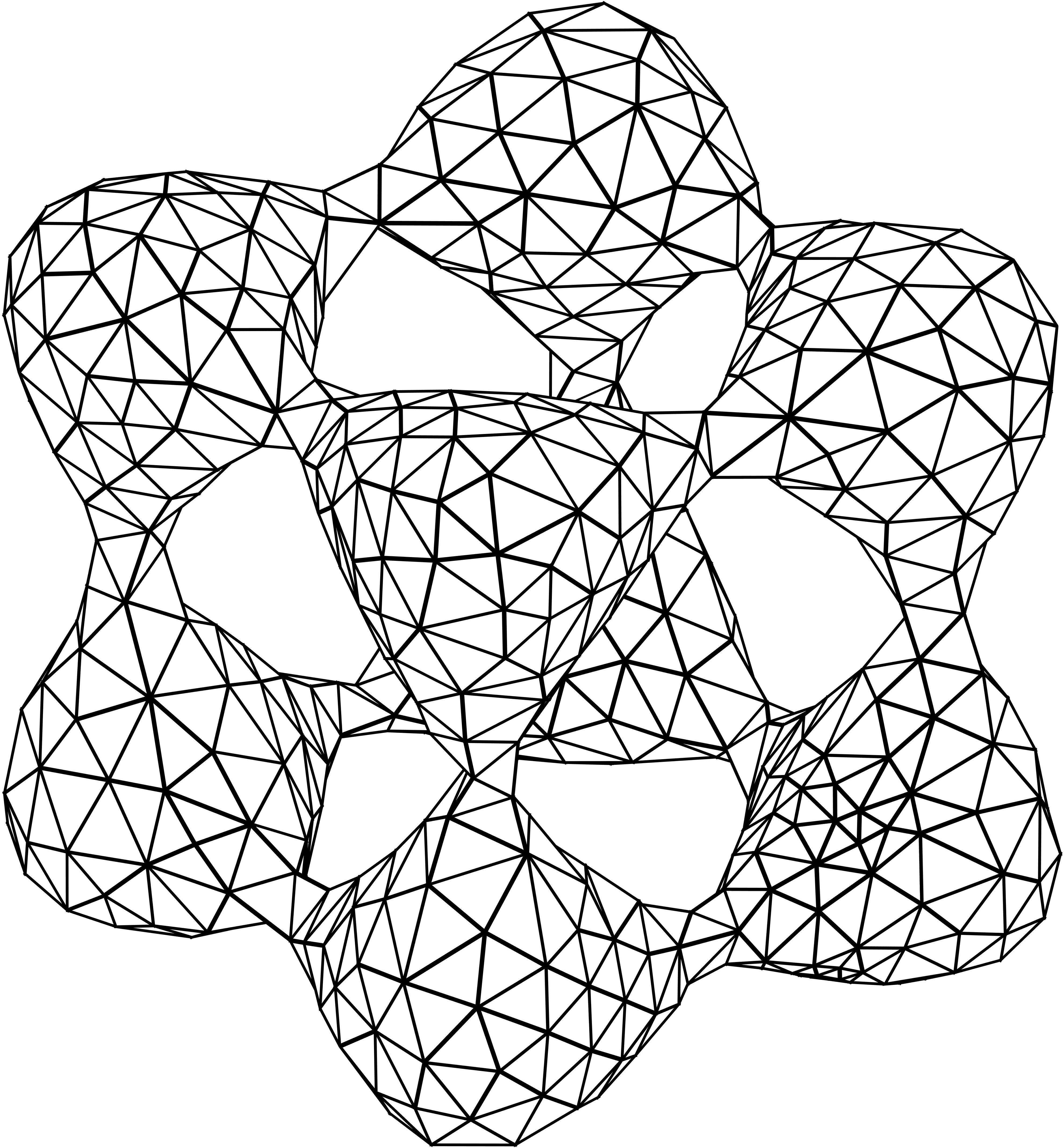
Figure 2: Initial mesh on a general surface

Table 5: Numerical results of solving Laplace-Beltrami equation on a general surface

Dof	$De$	Order	$De_{I}$	Order	$De_{r}$	Order	$De_{r_{2}}$	Order
701	1.32e+01	–	5.67e+00	–	1.12e+01	–	1.19e+01	–
2828	6.93e+00	0.93	1.67e+00	1.75	3.66e+00	1.61	3.68e+00	1.69
11336	3.52e+00	0.98	4.89e-01	1.77	1.04e+00	1.81	1.06e+00	1.80
45368	1.77e+00	0.99	1.34e-01	1.87	2.76e-01	1.91	2.88e-01	1.87
181496	8.86e-01	1.00	3.54e-02	1.92	7.12e-02	1.96	7.77e-02	1.89
726008	4.43e-01	1.00	9.21e-03	1.94	1.81e-02	1.98	2.15e-02	1.86

In this case, the vertices of the triangles $\mathcal{M}_{h}$ are located in the $\mathcal{O}(h^{2})$ range along with the normal directions of the exact surface. The first level of mesh is plotted in Figure 2. The history of numerical errors is documented in Table 5. As expected, we can observe the $\mathcal{O}(h)$ optimal convergence rate for the finite element gradient. The rate of $\mathcal{O}(h^{1.9})$ can be observed for the error between the finite element gradient and the gradient of the interpolation of the exact solution. Again, it means the mesh $\mathcal{M}_{h}$ satisfies the $\mathcal{O}(h^{2\sigma})$ irregular condition. As depicted by the Theorem 4.3, the recovered gradient using parametric polynomial preserving recovery is superconvergent to the exact gradient at the rate of $\mathcal{O}(h^{2})$ even though the vertices are not located on the exact surface. For parametric superconvergent patch recovery, it deteriorates a litter bit but we can still observe $\mathcal{O}(h^{1.86})$ superconvergence.

6.2 Optimal convergence of numerical solution for vector Laplace problems on triangulated surface discretization

In the test, we shall demonstrate the optimal convergence of finite element solutions of the vector Laplace problem on triangulated surface using linear element. The key ingredient is the usage of superconvergent recovered normal vectors. Before showing numerical results for vector Laplace problems, we use a numerical example to verify the superconvergence results of the recovered unit normal vectors using the idea of parametric polynomial recovery. Then we present a comparison study of the numerical solution of vector Laplace problem.

6.2.1 Reconstruction of normal vectors

In the example, we consider the torus surface as $\mathcal{M}$ whose sign distance function is

$$\Phi(x)=\sqrt{(\sqrt{x_{1}^{2}+x_{2}^{2}}-4)^{2}+x_{3}^{2}}-1.$$ (6.1)

Similar to [11], we firstly make a series of uniform meshes of Chevron pattern and map the meshes onto the torus. Let $\nu$ be the exact unit outer normal vector of $\mathcal{M}$. In practice, the information of $\nu$ is not available and we have to resort to the numerical approximation of $\nu$. In this test, we consider three different numerical approximation of $\nu$: the discrete elementwise unit outer normal vector $\nu_{h}$, the recovered unit outer normal vector $\bar{\nu}_{h}$ using weighted averaging, and the recovered unit outer normal vector $\nu^{r}_{h}$ using the recovered Jacobian from Algorithm 1 and formula (5.5). We compute the discrete maximal norm of the difference between the exact unit outer normal vector and its numerical approximations. The numerical results are summarized in Table 6. We can clearly observe that the recovered unit outer normal vector $\nu^{r}_{h}$ using Algorithm 1 converges to the exact unit outer normal vector at a superconvergent rate of $\mathcal{O}(h^{2})$ while the other two approximate only converge at an optimal rate of $\mathcal{O}(h)$.

Table 6: Numerical comparison of different approximate unit outer normal vector on Torus

NDof	$|\nu_{h}-\nu|_{\infty}$	Order	$|\bar{\nu}-\nu|_{\infty}$	Order	$|\nu_{h}^{r}-\nu|_{\infty}$	Order
200	1.49e-01	–	1.15e-01	–	5.14e-02	–
800	6.39e-02	1.23	5.54e-02	1.06	1.30e-02	1.99
3200	2.90e-02	1.14	2.69e-02	1.04	3.17e-03	2.04
12800	1.38e-02	1.07	1.33e-02	1.02	7.81e-04	2.02
51200	6.72e-03	1.04	6.59e-03	1.01	1.94e-04	2.01
204800	3.32e-03	1.02	3.28e-03	1.00	4.83e-05	2.00
819200	1.65e-03	1.01	1.64e-03	1.00	1.21e-05	2.00
3276800	8.21e-04	1.00	8.19e-04	1.00	3.01e-06	2.00

6.2.2 Numerical solution of vector Laplacian on unit sphere

In this test, we consider the numerical solution of vector Laplace problem (5.1). We choose the exact solution $u$ as

$$\mathbf{u}_{\tau}=\begin{bmatrix}-(y+z)x+y^{2}+z^{2}\\ -(x+z)y+x^{2}+z^{2}\\ -(x+y)z+x^{2}+y^{2}\end{bmatrix}$$ (6.2)

and the right hand side function can be computed from $u$. We use the linear surface finite element method to discretize the vector Laplacian with a penalty term [20]. Here, we adopt two different choice of unit normal vector in the penalty: one is the discrete elementwise normal vector $\nu_{h}$ and the other is the recovered unit normal vector $\nu_{h}^{r}$. The convergence history of $L_{2}$ error and $H_{1}$ error are plot in Figure 3. As observed in [20], $L_{2}$ and $H_{1}$ errors show no convergence rates with the discrete elementwise normal vector. However, optimal convergence for both $L_{2}$ and $H_{1}$ errors can be observed when the recovered unit normal vector $\nu_{h}^{r}$ is employed to the penalty.

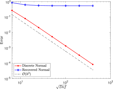
a

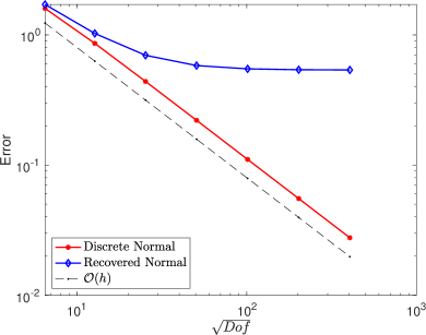
b

Figure 3: Numerical Results for the Vector Laplace-Beltrami equation on the unit sphere: (a) $L_{2}$ error on discrete surface; (b) $H_{1}$ error on discrete surface;.

7 Conclusion

In this paper, we have established a new concept called geometric supercloseness which is fundamental for analyzing the superconvergence of differential structure on manifolds. It is important for numerical analysis on deviated manifolds, particularly when there has no information of the exact geometry. In such cases, the vertices are typically not necessarily located on the underlying exact manifolds, and the exact normal vectors are not known. We focused on two implications. One is in post-processing of numerical solutions, that is superconvergence of gradient recovery methods on deviated discretized manifolds. It concludes the open questions proposed by Wei, Chen, and Huang. In the second case, we show that the superconvergence of differential structure can help in a priori error analysis of numerical solutions involving different structures, where we take tangential vector fields on manifolds as an example. The optimal convergence of the computed tangent vector field can be achieved without exact normal vectors. Although we have only investigated the condition for linear approximations, the higher-order cases are off course interesting as well, particularly the discretization assumptions which would lead to such conditions. On the other hand, for those problems whose solutions are tangent vector fields, we also need to investigate the case with deviated manifolds. In that case, we need to investigate superconvergence of curvature terms, which will be discussed in future work.

References

- [1] M. Ainsworth and J. T. Oden. A posteriori error estimation in finite element analysis. Pure and Applied Mathematics (New York). Wiley-Interscience [John Wiley & Sons], New York, 2000.
- [2] T. Aubin. Best constants in the Sobolev imbedding theorem: the Yamabe problem. In Seminar on Differential Geometry, volume 102 of Ann. of Math. Stud., pages 173–184. Princeton Univ. Press, Princeton, N.J., 1982.
- [3] R. E. Bank and J. Xu. Asymptotically exact a posteriori error estimators. I. Grids with superconvergence. SIAM J. Numer. Anal., 41(6):2294–2312 (electronic), 2003.
- [4] A. Bonito, A. Demlow, and R. H. Nochetto. Finite element methods for the laplace–beltrami operator. Handbook of Numerical Analysis. Elsevier, 2019.
- [5] S. C. Brenner and L. R. Scott. The mathematical theory of finite element methods, volume 15 of Texts in Applied Mathematics. Springer, New York, third edition, 2008.
- [6] H. Chen, H. Guo, Z. Zhang, and Q. Zou. A linear finite element method for two fourth-order eigenvalue problems. IMA J. Numer. Anal., 37(4):2120–2138, 2017.
- [7] P. G. Ciarlet. The finite element method for elliptic problems, volume 40 of Classics in Applied Mathematics. Society for Industrial and Applied Mathematics (SIAM), Philadelphia, PA, 2002. Reprint of the 1978 original [North-Holland, Amsterdam; MR0520174 (58 #25001)].
- [8] A. Demlow. Higher-order finite element methods and pointwise error estimates for elliptic problems on surfaces. SIAM J. Numer. Anal., 47(2):805–827, 2009.
- [9] A. Demlow and G. Dziuk. An adaptive finite element method for the Laplace-Beltrami operator on implicitly defined surfaces. SIAM J. Numer. Anal., 45(1):421–442 (electronic), 2007.
- [10] M. P. do Carmo. Riemannian geometry. Mathematics: Theory & Applications. Birkhäuser Boston, Inc., Boston, MA, 1992. Translated from the second Portuguese edition by Francis Flaherty.
- [11] G. Dong and H. Guo. Parametric polynomial preserving recovery on manifolds. arXiv preprint 1703.06509, pages 1 – 27, 2017.
- [12] G. Dong, B. Jüttler, O. Scherzer, and T. Takacs. Convergence of Tikhonov regularization for solving ill–posed operator equations with solutions defined on surfaces. Inverse Probl. Imaging, 11(2):221 – 246, 2017.
- [13] Q. Du and L. Ju. Finite volume methods on spheres and spherical centroidal Voronoi meshes. SIAM J. Numer. Anal., 43(4):1673–1692 (electronic), 2005.
- [14] G. Dziuk. Finite elements for the Beltrami operator on arbitrary surfaces. In Partial differential equations and calculus of variations, volume 1357 of Lecture Notes in Math., pages 142–155. Springer, Berlin, 1988.
- [15] G. Dziuk and C. M. Elliott. Finite element methods for surface PDEs. Acta Numer., 22:289–396, 2013.
- [16] S. Gross, T Jankuhn, M. A. Olshanskii, and A. Reusken. A trace finite element method for vector-Laplacians on surfaces. SIAM J. Numer. Anal., 56(4):2406–2429, 2018.
- [17] H. Guo, C. Xie, and R. Zhao. Superconvergent gradient recovery for virtual element methods. Math. Models Methods Appl. Sci., 29(11):2007–2031, 2019.
- [18] H. Guo, Z. Zhang, and R. Zhao. Hessian recovery for finite element methods. Math. Comp., 86(306):1671–1692, 2017.
- [19] H. Guo, Z. Zhang, and Q Zou. A Linear Finite Element Method for Biharmonic Problems. J. Sci. Comput., 74(3):1397–1422, 2018.
- [20] M.G. Hansbo, P.and Larson and K. Larsson. Analysis of finite element methods for vector Laplacians on surfaces. IMA J. Numer. Anal., 00:1–50, 2019.
- [21] M.W. Hirsch. Differential Topology, volume Graduate Texts in Mathematics (33). Springer, 1976.
- [22] A. M. Lakhany, I. Marek, and J. R. Whiteman. Superconvergence results on mildly structured triangulations. Comput. Methods Appl. Mech. Engrg., 189(1):1–75, 2000.
- [23] A. Naga and Z. Zhang. A posteriori error estimates based on the polynomial preserving recovery. SIAM J. Numer. Anal., 42(4):1780–1800 (electronic), 2004.
- [24] A. Naga and Z. Zhang. Function value recovery and its application in eigenvalue problems. SIAM J. Numer. Anal., 50(1):272–286, 2012.
- [25] A. Naga, Z. Zhang, and A. Zhou. Enhancing eigenvalue approximation by gradient recovery. SIAM J. Sci. Comput., 28(4):1289–1300, 2006.
- [26] M. A. Olshanskii, A. Quaini, A. Reusken, and V. Yushutin. A finite element method for the surface stokes problem. SIAM J. Sci. Comput., 40(4):2492–2518, 2018.
- [27] S. Reuther and A. Voigt. Solving the incompressible surface navier-stokes equation by surface finite elements. Physics of Fluids, 30(1):012107, 2018.
- [28] L. Rineau and M. Yvinec. 3D surface mesh generation. In CGAL User and Reference Manual. CGAL Editorial Board, 4.9 edition, 2016.
- [29] H. Wei, L. Chen, and Y. Huang. Superconvergence and gradient recovery of linear finite elements for the Laplace-Beltrami operator on general surfaces. SIAM J. Numer. Anal., 48(5):1920–1943, 2010.
- [30] J. Xu and Z. Zhang. Analysis of recovery type a posteriori error estimators for mildly structured grids. Math. Comp., 73(247):1139–1152 (electronic), 2004.
- [31] Z. Zhang and A. Naga. A new finite element gradient recovery method: superconvergence property. SIAM J. Sci. Comput., 26(4):1192–1213 (electronic), 2005.
- [32] O. C. Zienkiewicz and J. Z. Zhu. The superconvergent patch recovery and a posteriori error estimates. I. The recovery technique. Internat. J. Numer. Methods Engrg., 33(7):1331–1364, 1992.
- [33] O. C. Zienkiewicz and J. Z. Zhu. The superconvergent patch recovery and a posteriori error estimates. II. Error estimates and adaptivity. Internat. J. Numer. Methods Engrg., 33(7):1365–1382, 1992.