Laplacian Smoothing Stochastic Gradient Markov Chain Monte Carlo

Abstract

As an important Markov Chain Monte Carlo (MCMC) method, stochastic gradient Langevin dynamics (SGLD) algorithm has achieved great success in Bayesian learning and posterior sampling. However, SGLD typically suffers from slow convergence rate due to its large variance caused by the stochastic gradient. In order to alleviate these drawbacks, we leverage the recently developed Laplacian Smoothing (LS) technique and propose a Laplacian smoothing stochastic gradient Langevin dynamics (LS-SGLD) algorithm. We prove that for sampling from both log-concave and non-log-concave densities, LS-SGLD achieves strictly smaller discretization error in $2$-Wasserstein distance, although its mixing rate can be slightly slower. Experiments on both synthetic and real datasets verify our theoretical results, and demonstrate the superior performance of LS-SGLD on different machine learning tasks including posterior sampling, Bayesian logistic regression and training Bayesian convolutional neural networks. The code is available at https://github.com/BaoWangMath/LS-MCMC.

1 Introduction

Given a dataset $\mathcal{D}=\{{\bm{d}}_{i}\}_{i=1}^{n}$, the posterior of a machine learning (ML) model’s parameters ${\bm{x}}\in{\mathbb{R}}^{d}$ with prior $p({\bm{x}})$ and likelihood $\Pi_{i=1}^{n}p({\bm{d}}_{i}|{\bm{x}})$ is computed as $p({\bm{x}}|\mathcal{D})\propto p({\bm{x}})\Pi_{i=1}^{n}p({\bm{d}}_{i}|{\bm{x}})$. Optimization algorithms are used to find the maximum a posterior (MAP) estimate, ${\bm{x}}_{\rm MAP}=\operatorname*{arg\,max}_{\bm{x}}\log p({\bm{x}}|\mathcal{D})$. Sampling algorithms such as Langevin Dynamics (LD) are used to sample the posterior or the log posterior. In this paper, we consider applying LD-based MCMC algorithms to sample $e^{-f({\bm{x}})}$, where

$$f({\bm{x}}):=\frac{1}{n}\sum_{i=1}^{n}f_{i}({\bm{x}})=-\frac{1}{n}\sum_{i=1}^{n}\log p({\bm{d}}_{i}|{\bm{x}}).$$ (1)

Here, we normalized the log-likelihood by a factor $n$ for the ease of presentation in the remaining part of this paper.

The first-order LD reads:

$$d{\bm{X}}_{t}=-\nabla f({\bm{X}}_{t})\text{d}t+\sqrt{2\beta^{-1}}\cdot\text{d}{\bm{B}}_{t},$$ (2)

where ${\bm{X}}_{t}\in{\mathbb{R}}^{d}$ denotes the point at time $t$, $\beta$ denotes the inverse temperature and ${\bm{B}}_{t}\in{\mathbb{R}}^{d}$ is the standard Brownian term. Under certain assumptions on the negative log posterior (i.e., $f({\bm{x}})$), the LD (2) converges to an unique invariant distribution $\pi\propto e^{-\beta f({\bm{x}})}$ (Chiang et al., 1987). Therefore, one can apply numerical integrator to approximate (2) in order to obtain samples that follow the posterior distribution. One simple integrator is to apply the Euler-Maruyama discretization (abd E. Platen, 1992) to (2), which gives:

$${\bm{x}}_{k+1}={\bm{x}}_{k}-\eta\nabla f({\bm{x}}_{k})+\sqrt{2\beta^{-1}\eta}\cdot{\bm{\epsilon}}_{k},$$ (3)

and it is known as the Langevin Monte Carlo (LMC), (a.k.a., unadjusted Langevin algorithm (Parisi, 1981)). When the target density, i.e., posterior distribution, is strongly log-concave and log-smooth, Dalalyan (2017); Durmus et al. (2017) proved that LMC is able to converge to the target density up to an arbitrarily small sampling error in both total variation and $2$-Wasserstein distances. Furthermore, the convergence guarantee of LMC for sampling from non-log-concave distributions has also been established in Raginsky et al. (2017); Xu et al. (2018).

Note that the posterior distribution is defined on the whole dataset $\mathcal{D}$, which is typically extremely large in modern ML tasks. Therefore, computing the full gradient $\nabla f({\bm{x}})$ is inefficient and may dramatically slow down the convergence of sampling algorithms. One solution is to replace the full gradient in (3) with a subsampled one, which gives rise to Stochastic Gradient Langevin Dynamics (SGLD) (Welling and Whye, 2011). From the theoretical perspective, the convergence guarantee of SGLD has been proved for both strongly log-concave distributions (Dalalyan and Karagulyan, 2017) and non-log-concave distributions (Raginsky et al., 2017; Xu et al., 2018) in $2$- Wasserstein distance. Mou et al. (2017) further studied the generalization performance of SGLD for nonconvex optimization. Although SGLD can drastically reduce the computational cost, it is also observed to have a slow convergence rate due to the large variance caused by the stochastic gradient (Teh et al., 2016; Vollmer et al., 2016). In order to reduce the variance of stochastic gradient as well as to improve the convergence rate, Dubey et al. (2016) incorporated variance reduction techniques into SGLD, which gives rise to a family of variance-reduced LD-based algorithms such as SVRG-LD and SAGA-LD. Chatterji et al. (2018); Zou et al. (2018b, 2019a) further proved that SVRG-LD and SAGA-LD are able to converge to the target density with fewer stochastic gradient evaluations than SGLD and LMC in certain regimes. However, both SVRG-LD and SAGA-LD require a large amount of extra computation and memory costs and can only be shown to achieve faster convergence on small to moderate datasets. Therefore, it is natural to ask if we can reduce the variance of stochastic gradients while maintaining similar computation and memory costs of SGLD?

Recently, Osher et al. (2018) integrated Laplacian smoothing and related high-order smoothing techniques into Stochastic Gradient Descent (SGD) to reduce the variance of stochastic gradient on-the-fly. Laplacian Smoothing SGD (LSSGD) allows us to take a significantly larger step size than vanilla SGD and reduces the optimality gap in convex optimization when constant step size is used. Empirically, LSSGD preconditions the gradient when the objective function has a large condition number and can avoid local minima. Because of this, LSSGD is applicable to train a large number of deep learning models with good generalizability. Laplacian smoothing also demonstrates some ability to avoid saddle point in gradient descent (Kreusser et al., 2019). Most recently, Wang et al. (2019) leveraged Laplacian smoothing to improve the utility of machine learning models trained with privacy guarantee.

In this paper, we integrate Laplacian smoothing with SGLD, and we call the resulting algorithm Laplacian Smoothing SGLD (LS-SGLD). The extra computation of LS-SGLD compared with SGLD is that we need to compute the products of the inverse of two circulant matrices with vectors. We leverage the Fast Fourier Transform to develop fast algorithms to compute these matrix-vector products efficiently, and the resulting algorithms can compute the matrix-vector products with a negligible overhead in both time and memory.

1.1 Our Contributions

We summarize the main contributions of this work as follows:

• We propose a simple modification on the SGLD, which applies the Laplacian smoothing matrix and its squared root to the stochastic gradient and Gaussian noise vectors, respectively. The continuous and full-gradient counter-part of the modified LS-SGLD has the same stationary distribution as the LD.

• We proposed FFT-based fast algorithms to compute the product of the inverse of circulant matrices with any given vector. By leveraging the structure of eigenvalues and eigenvectors of the circulant matrices, we can compute these products very efficiently with a negligible overhead in both time and memory.

• We prove the convergence rate of LS-SGLD for sampling from both log-concave and non-log-concave densities in $2$-Wasserstein distance. Specifically, we decompose the sampling error into the discretization error and the ergodicity rate. Moreover, we show that there exists a trade-off between the discretization error and ergodicity rate of LS-SGLD, as adding Laplacian smoothing can reduce the discretization error but slow down the mixing time.

• We conduct extensive experiments to evaluate the performance of LS-SGLD. First, we show that compared with SGLD, LS-SGLD can achieve a significantly smaller discretization error but similar ergodicity rate, which implies that the overall sampling error of LS-SGLD can be much smaller. Second, we conduct experiments on both synthetic and real data for posterior sampling, Bayesian logistic regression and training Bayesian convolutional networks, all of which demonstrate the superior performance of LS-SGLD.

1.2 Additional Related Work

In addition to the first-order Langevin based algorithms we discussed in the introduction, there also emerges a vast body of work focusing on higher-order Langevin based algorithms. One of the well-know high-order MCMC method is Hamiltonian Monte Carlo (HMC) (Neal et al., 2011), which incorporates an Hamiltonian momentum term into the first-order MCMC method in order to improve the mixing time. Similar to SGLD, a stochastic version of HMC (namely SGHMC) has been further established in Chen et al. (2014), which was shown to be able to achieve a faster convergence rate than SGLD in experiments. Ma et al. (2015) investigated a family of SGHMC methods and proposed a new state-adaptive sampler on the Riemannian manifold. Chen et al. (2015) provided theoretical convergence guarantees of SGHMC in terms of mean square error (MSE) and proposed a 2nd-order symmetric splitting integrator to further improve the discretization error. When the target density is strongly log-concave and log-smooth, Cheng et al. (2018b) proposed underdamped MCMC (U-MCMC) and stochastic underdamped MCMC (SG-U-MCMC), and obtained convergence rates in $2$-Wasserstein distance. The convergence rates of these two algorithms have been further established for sampling from non-log-concave densities (Cheng et al., 2018a). However, due to the large variance of stochastic gradients and lacking of the Metropolis Hasting (MH) correction step, SGHMC has also been observed to have highly biased sampling trajectory (Betancourt, 2015; Dang et al., 2019). One way to address this issue is to make use of a variance-reduction technique to alleviate the variance of stochastic gradients in SGHMC, which gave rise to stochastic variance-reduced HMC methods (Zou et al., 2018a; Li et al., 2018; Zou et al., 2019b).

1.3 Organization

We organize this paper as follows: We present LS-SGLD and derive FFT-based fast algorithms for LS-SGLD in Section 2. In Section 3, we give theoretical guarantees for the performance of LS-SGLD in both log-concave and non-log-concave settings. In Section 4, we numerically verify the performance of LS-SGLD on sampling different distributions, training Bayesian logistic regression, and convolutional neural nets. We conclude this work in Section 5.

1.4 Notations

Throughout this paper we use bold upper-case letters ${\mathbf{A}}$, ${\mathbf{B}}$ to denote matrices, bold lower-case letters ${\bm{x}}$, ${\bm{y}}$ to denote vectors, and lower cases letters $x$, $y$ and $\alpha$, $\beta$ to denote scalars. For continuous-time random vectors, we denote them with the tilt bold upper-case letters ${\bm{X}}$, ${\bm{Y}}$ with sub/super-scripts. For vector ${\bm{x}}=(x_{1},\dots,x_{d})^{\top}$, we use $\|{\bm{x}}\|_{2}=\sqrt{x_{1}^{2}+\dots+x_{d}^{2}}$ to represent its $\ell_{2}$-norm and use $\|{\bm{x}}\|_{{\mathbf{A}}}=\sqrt{{\bm{x}}^{\top}{\mathbf{A}}{\bm{x}}}$ to represent its ${\mathbf{A}}$-norm, where ${\mathbf{A}}$ is an semi-positive definite matrix. We use ${\mathbb{P}}({\bm{x}})$ to denote the distribution of ${\bm{x}}$, and ${\mathcal{W}}_{2}(\cdot,\cdot)$ and $D_{KL}(\cdot||\cdot)$ denote the $2$-Wasserstein distance and Kullback–Leibler (KL) divergence between two distributions, respectively. For a function $f:{\mathbb{R}}^{d}\rightarrow{\mathbb{R}}$, we use $\nabla f(\cdot)$ and $\nabla^{2}f(\cdot)$ to denote its gradient and Hessian.

2 Algorithms

2.1 Laplacian Smoothing (Stochastic) Gradient Descent

For $\sigma\geq 0$, let ${\mathbf{A}}_{\sigma}:={\mathbf{I}}-\sigma\mathbf{L}$ where ${\mathbf{I}}\in{\mathbb{R}}^{d\times d}$ and $\mathbf{L}\in{\mathbb{R}}^{d\times d}$ are the identity and the discrete one-dimensional Laplacian matrix, respectively. Therefore,

$${\mathbf{A}}_{\sigma}:=\begin{bmatrix}1+2\sigma&-\sigma&0&\dots&0&-\sigma\\ -\sigma&1+2\sigma&-\sigma&\dots&0&0\\ 0&-\sigma&1+2\sigma&\dots&0&0\\ \dots&\dots&\dots&\dots&\dots&\dots\\ -\sigma&0&0&\dots&-\sigma&1+2\sigma\end{bmatrix}_{d\times d}$$ (4)

To find ${\bm{x}}_{\rm MAP}$ of (1), LSSGD (Osher et al., 2018) takes the following iteration

$${\bm{x}}^{k+1}={\bm{x}}^{k}-\eta_{k}{\mathbf{A}}_{\sigma}^{-1}\nabla f_{i_{k}}({\bm{x}}^{k}),$$ (5)

where $\eta_{k}>0$ is the learning rate, $i_{k}$ is a random sample from $[n]:=\{1,2,\cdots,n\}$. When $\sigma=0$, LSSGD reduces to SGD. Since ${\mathbf{A}}_{\sigma}$ is a circulant matrix, for any vector ${\bm{v}}$, ${\mathbf{A}}_{\sigma}^{-1}{\bm{v}}:={\bm{u}}$ can be computed via the FFT in the following way

$${\mathbf{A}}_{\sigma}^{-1}{\bm{v}}={\bm{u}}\Longrightarrow{\bm{v}}={\mathbf{A}}_{\sigma}{\bm{u}}={\bm{u}}-\sigma{\bm{d}}*{\bm{u}},$$

where $*$ is the convolution operator, and ${\bm{d}}=[-2,1,0,\cdots,0,1]^{T}$. By the convolution theorem, we have

$${\rm fft}({\bm{v}})={\rm fft}({\bm{u}})-\sigma{\rm fft}({\bm{d}}){\rm fft}({\bm{u}}).$$

Finally, we arrive at the following FFT-based algorithm for computing ${\mathbf{A}}_{\sigma}^{-1}{\bm{v}}$

$${\mathbf{A}}_{\sigma}^{-1}{\bm{v}}={\rm ifft}\left(\frac{{\rm fft}({\bm{v}})}{\mathbf{1}-\sigma\cdot{\rm fft}({\bm{d}})}\right),$$

where $\mathbf{1}$ is an all-one vector with the same dimension as ${\bm{v}}$, and the division of two vectors is defined in the coordinate-wise way. fft and ifft denote FFT and inverse FFT operators, respectively.

The Laplacian matrix ${\mathbf{A}}_{\sigma}^{-1}$ can reduce the variance of stochastic gradient and guarantee at least the same convergence rate as SGD. Osher et al. (2018) showed that for a $L$-gradient Lipschitz function $f({\bm{x}})$, i.e., $\|\nabla f({\bm{x}})\|_{2}\leq L$, the largest step size for LSSGD is $(1+4\sigma)^{1/4}/L$ (with high probability) which is larger than GD’s by a factor $(1+4\sigma)^{1/4}$.

2.2 Laplacian Smoothing Langevin Dynamics

We integrate Laplacian smoothing with LD and obtain the following Lapacian Smoothing LD (LS-LD)

$$d{\bm{X}}_{t}=-{\mathbf{A}}_{\sigma}^{-1}\nabla f({\bm{X}}_{t})+\sqrt{2\beta^{-1}}{\mathbf{A}}_{\sigma}^{-1/2}\text{d}{\bm{B}}_{t}.$$ (6)

Note that we pre-multiply the Brownian motion term by ${\mathbf{A}}_{\sigma}^{-1/2}$ instead of ${\mathbf{A}}_{\sigma}^{-1}$ to guarantee that the stationary distribution of the LS-LD remains to be $\exp{\left(-\beta f({\bm{x}})\right)}$. We can easily verify that LD and LS-LD have the same stationary distribution by looking at the associated Fokker-Planck equation. We formally state this property in the following proposition.

Proposition 1.

The stationary distribution, $\pi$, of the LS-LD, (6), satisfies $\pi\propto e^{-\beta f({\bm{x}})}$.

If we apply the Euler-Maruyama scheme to discretize (6), we end up with the following discrete algorithm, namely Laplacian smoothing gradient Langevin dynamics (LS-GLD)

$${\bm{x}}_{k+1}={\bm{x}}_{k}-\eta{\mathbf{A}}_{\sigma}^{-1}\nabla f({\bm{x}}_{k})+\sqrt{2\beta^{-1}\eta}{\mathbf{A}}_{\sigma}^{-1/2}\bm{\epsilon}_{k},$$ (7)

where $\bm{\epsilon}_{k}\sim N(\mathbf{0},{\mathbf{I}}_{d\times d})$. In practice, we use the mini-batch gradient ${\mathbf{g}}_{k}=\sum_{i\in\mathcal{I}_{k}}\nabla f_{i}({\bm{x}}_{k})/|\mathcal{I}_{k}|$ with $\mathcal{I}_{k}\subset[n]$ to replace the gradient in (7), and we arrive at the following LS-SGLD

$${\bm{x}}_{k+1}={\bm{x}}_{k}-\eta{\mathbf{A}}_{\sigma}^{-1}{\mathbf{g}}_{k}+\sqrt{2\beta^{-1}\eta}{\mathbf{A}}_{\sigma}^{-1/2}\bm{\epsilon}_{k}.$$ (8)

We summarize LS-SGLD in Algorithm 1. It is worth noting that computing the inverse of both ${\mathbf{A}}_{\sigma}$ and ${\mathbf{A}}_{\sigma}^{1/2}$ can be expensive. Moreover, multiplying the vectors by the inverse of these two matrices is also expensive. So in the remaining part of this section, we will present FFT-based fast algorithms for implementing (7).

Algorithm 1 LS-SGLD

Input: Training data, learning rate $\eta$, minibatch size $B$, inverse temperature $\beta$, Laplacian smoothing constant $\sigma$.

Initialization: Set ${\bm{x}}_{0}=0$.

for $k=0,1,\cdots,K-1$ do

     Uniformly sample $\mathcal{I}_{k}\subset[n]$ with $|\mathcal{I}_{k}|=B$.

     Compute the mini-batch stochastic gradient $\sum_{i\in\mathcal{I}_{k}}\nabla f_{i}({\bm{x}}_{k})/B$.

     ${\bm{x}}_{k+1}={\bm{x}}_{k}-\eta{\mathbf{A}}_{\sigma}^{-1}{\mathbf{g}}_{k}+\sqrt{2\beta^{-1}\eta}{\mathbf{A}}^{-1/2}_{\sigma}\bm{\epsilon}_{k}$, where $\bm{\epsilon}_{k}\sim N(\mathbf{0},\mathbf{I}_{d\times d})$.

Output: ${\bm{x}}_{0},\dots,{\bm{x}}_{K}$.

2.3 FFT-based Implementation of LS-SGLD

2.3.1 Circulant Matrix and Convolutional Operation

In this subsection, we list a few results on the circulant matrix which will be the basic recipes for designing FFT-based algorithm to solving (7).

Lemma 1 (Golub and Van Loan (1996)).

The normalized eigenvectors of the following $d\times d$ circulant matrix,

$$\mathbf{C}=\begin{bmatrix}c_{0}&c_{d-1}&\dots&c_{2}&c_{1}\\ c_{1}&c_{0}&c_{d-1}&\dots&c_{2}\\ \dots&\dots&\dots&\dots&\dots\\ c_{d-2}&\dots&\dots&\dots&c_{d-1}\\ c_{d-1}&c_{d-2}&\dots&c_{1}&c_{0}\end{bmatrix},$$ (9)

are given by

$${\bm{v}}_{j}=\frac{1}{\sqrt{d}}\left(1,w_{j},w_{j}^{2},\cdots,w_{j}^{n-1}\right),\ \ j=0,1,\cdots,d-1,$$

where $w_{j}=\exp\left(i\frac{2\pi j}{d}\right)$ are the $j$-th roots of unity and $i$ is the imaginary unit. The corresponding eigenvalues are then given by

$$\lambda_{j}=c_{0}+c_{d-1}w_{j}+c_{d-2}w_{j}^{2}+\cdots+c_{1}w_{j}^{d-1},\ \ \ j=0,1,\cdots,d-1.$$

Lemma 2 (Golub and Van Loan (1996)).

The inverse of a circulant matrix is circulant.

Lemma 3 (Golub and Van Loan (1996)).

The square root of a circulant matrix is circulant.

Lemma 4.

For any circulant matrix $\mathbf{C}$ of the form in (9), and for any given vector ${\bm{v}}$. Let ${\bm{u}}=\mathbf{C}^{-1}{\bm{v}}$, then ${\bm{u}}$ can be computed by the fast Fourier transform with sublinear scaling in the following way

$${\bm{u}}={\rm ifft}\left(\frac{{\rm fft}({\bm{v}})}{{\rm fft}({\bm{c}})}\right),$$ (10)

where ${\bm{c}}$ is the first row of the matrix $\mathbf{C}$, and the division in (10) is defined coordinate-wise.

Proof.

Since $\mathbf{C}$ is a circulant matrix we have ${\bm{v}}=\mathbf{C}{\bm{u}}={\bm{c}}*{\bm{u}}$, therefore ${\rm fft}({\bm{v}})={\rm fft}({\bm{c}})\cdot{\rm fft}({\bm{u}})$. ∎

2.3.2 Fast Algorithm for Computing the Square Root of Laplacian Smoothing

We will derive an FFT-based algorithm for computing ${\mathbf{A}}_{\sigma}^{-1/2}\bm{\epsilon}_{k}$ in this subsection. According to Lemmas 2 and 3, ${\mathbf{A}}_{\sigma}^{-1/2}$ is circulant. Note ${\mathbf{A}}_{\sigma}^{-1}$ is positive definite, we denote its eigen-decomposition as

$${\mathbf{A}}_{\sigma}^{-1}={\mathbf{Q}}\Lambda{\mathbf{Q}}^{-1},$$

where ${\mathbf{Q}}=[{\bm{v}}_{1},{\bm{v}}_{2},\cdots,{\bm{v}}_{d}]^{T}$ with ${\bm{v}}_{i}$ being the eigenvector associated with the eigenvalue $\lambda_{i}>0$, and $\Lambda={\rm diag}(\lambda_{1},\lambda_{2},\cdots,\lambda_{d})$. Therefore, we have

$${\mathbf{A}}_{\sigma}^{-1/2}={\mathbf{Q}}\sqrt{\Lambda}{\mathbf{Q}}^{-1},$$ (11)

where $\sqrt{\Lambda}={\rm diag}(\sqrt{\lambda_{1}},\sqrt{\lambda_{2}},\cdots,\sqrt{\lambda_{d}})$.

Furthermore, note that ${\mathbf{A}}_{\sigma}$ is symmetric, therefore ${\mathbf{Q}}^{-1}={\mathbf{Q}}^{T}$. It follows that we can compute ${\mathbf{A}}^{-1/2}_{\sigma}$ without inverting the matrix ${\mathbf{Q}}$. By the fact that ${\mathbf{A}}_{\sigma}^{-1/2}$ is circulant, we have ${\mathbf{A}}_{\sigma}^{-1/2}\bm{\epsilon}_{k}={\rm ifft}({\rm fft}({\bm{b}})\cdot{\rm fft}(\bm{\epsilon}_{k}))$, where ${\bm{b}}$ is the first row of ${\mathbf{A}}_{\sigma}^{-1/2}$.

Remark 1.

In computing (11), there is no need to store the matrix ${\mathbf{Q}}$, according to Lemma 1, each row of ${\mathbf{Q}}$ and $\sqrt{\Lambda}$ can be written down explicitly which enables us to compute ${\mathbf{A}}_{\sigma}^{-1/2}$ quickly with negligible memory overhead and scalable to very high dimensional problems.

3 Main Results

We first make the following three assumptions regarding the function $f({\bm{x}})$.

Assumption 1 (Dissipativeness).

For any ${\bm{x}}\in{\mathbb{R}}^{d}$, there exist constants $m$ and $b$ such that

$$\langle\nabla f({\bm{x}}),{\bm{x}}\rangle\geq m\|{\bm{x}}\|_{2}^{2}-b.$$

This assumption has been widely made to study the convergence of Langevin based sampling algorithms (Mattingly et al., 2002; Raginsky et al., 2017; Xu et al., 2018; Zou et al., 2019a), which is essential to guarantee the convergence of the continuous-time Langenvin dynamics (2).

Assumption 2 (smoothness).

For any ${\bm{x}},{\bm{y}}\in{\mathbb{R}}^{d}$, there exists a positive constant $M$ such that for all $i=1,\dots,n$, it holds that

$$\|\nabla f_{i}({\bm{x}})-\nabla f_{i}({\bm{y}})\|_{2}\leq M\|{\bm{x}}-{\bm{y}}\|_{2}.$$

Unlike Assumption 1, Assumption 2 is made for all component function $f_{i}({\bm{x}})$.

Assumption 3 (Bounded Variance).

For any ${\bm{x}}\in{\mathbb{R}}^{d}$, there exists a constant $\omega$ such that the variance of the stochastic gradient is bounded as follows,

$${\mathbb{E}}[\|\nabla f_{i}({\bm{x}})-\nabla f({\bm{x}})\|_{2}^{2}]\leq d\omega^{2}.$$

Definition 1 (Logarithmic Sobolev inequality).

Let $\mu$ be a probability measure, then we say $\mu$ satisfies logarithmic Sobolev inequality with constant $\lambda$ if for any smooth function $g$, the following holds:

$$\int g^{2}\log g^{2}\text{d}\mu-\int g^{2}\text{d}\mu\log\int g^{2}\text{d}\mu\leq\lambda\int\|\nabla g\|_{2}^{2}\text{d}\mu.$$

Then the following proposition states that if the function $f(\cdot)$ satisfies Assumptions 1 and 2, the target density $\pi\propto e^{-f({\bm{x}})}$ satisfies Logarithmic Sobolev inequality.

Proposition 2 (Raginsky et al. (2017)).

Under Assumptions 1 and 2, the target density $\pi\propto e^{-f({\bm{x}})}$ satisfies Logarithmic Sobolev inequality with some constant $\lambda>0$.

It has been shown in Durmus et al. (2017); Raginsky et al. (2017) that if the function $f({\bm{x}})$ is smooth and strongly convex (which is stronger than Assumption 1), the logarithmic Sobolev constant $\lambda$ is an universal constant. However, if the function $f({\bm{x}})$ is nonconvex, in the worst case the logarithm Sobolev constant $\lambda$ can have exponential dependency on the problem dimension $d$ and inverse temperature $\beta$ (Bovier et al., 2004; Raginsky et al., 2017).

3.1 Convergence Analysis of Sampling from Log-concave Densities

In this subsection, we assume that the target density is log-concave, which is equivalent to the following assumption on the function $f({\bm{x}})$.

Assumption 4 (Convexity).

For any ${\bm{x}},{\bm{y}}\in{\mathbb{R}}^{d}$, it holds that

$$f({\bm{x}})-f({\bm{y}})\geq\langle\nabla f({\bm{y}}),{\bm{x}}-{\bm{y}}\rangle.$$

Then we are ready to establish the convergence rate of LS-SGLD for sampling from log-concave densities, which is stated in the following theorem.

Theorem 1.

Under Assumptions 1, 2, 3 and 4, if set the step size $\eta\leq Cm\beta^{-1}/M^{2}$ for some sufficiently small constant $C$, there exist constants $c_{0}\in[\|{\mathbf{A}}_{\sigma}\|_{2}^{-1},1]$, $\gamma_{1}\in[\|{\mathbf{A}}_{\sigma}\|_{2}^{-2},1]$ and $\gamma_{2}=d^{-1}\sum_{i=1}^{d}(1+2\sigma-2\sigma\cos(2\pi i/d))^{-1}$ such that the output of LS-SGLD satisfies,

$${\mathcal{W}}_{2}({\mathbb{P}}({\bm{x}}_{K}),\pi)\leq\bigg{(}\frac{2\gamma_{1}K\eta^{2}\beta d\omega^{2}}{B}\bigg{)}^{1/2}+\big{[}8\gamma_{2}K\eta^{2}\cdot(K+1)\beta d\eta\big{]}^{1/2}+\big{[}2\lambda\big{(}\beta f(0)+\log(\Lambda)\big{)}\big{]}^{1/2}\cdot e^{-c_{0}K\eta/(2\beta\lambda)},$$ (12)

where $\Lambda=\int_{{\mathbb{R}}^{d}}e^{-\beta f({\bm{x}})}\text{d}{\bm{x}}$ and $\lambda$ denotes the logarithmic Sobolev constant of the target distribution $\pi\propto e^{-\beta f({\bm{x}})}$.

Table 1: The values of $\gamma_{2}$ corresponding to some $\sigma$ and $d$.

$\sigma$	1	2	3	4	5
$d=1000$	0.268	0.185	0.149	0.128	0.114
$d=10000$	0.268	0.185	0.149	0.128	0.114
$d=100000$	0.268	0.185	0.149	0.128	0.114

Remark 2.

We emphasize that the the three terms on the R.H.S. of (12) have their respective meanings. In particular, the first and second terms represent the discretization errors introduced by stochastic gradient estimator and numerical integrator of (6), respectively. The third term represents the ergodicity of the continuous-time Markov process (6), which characterizes the mixing time of LS-LD (6). Moreover, we remark here that the convergence rate of LS-GLD (LS-SGLD with full gradient) can be directly implied from Theorem 1 by removing the first term on the R.H.S. of (12).

Based on Theorem 1, we can also derive the convergence rate of SGLD in the same setting by setting ${\mathbf{A}}_{\sigma}={\mathbf{I}}$ (i.e., $\sigma=0$), which implies that the constants $\gamma_{1},\gamma_{2}$ and $c_{0}$ in Theorem 1 are all $1$’s. We formally state the convergence result of SGLD in the following corollary.

Corollary 1.

Under the same assumptions in Theorem 1, the output of standard SGLD, denoted by ${\bm{y}}_{K}$, satisfies

$${\mathcal{W}}_{2}({\mathbb{P}}({\bm{y}}_{K}),\pi)\leq\bigg{(}\frac{2K\eta^{2}d\omega^{2}}{B}\bigg{)}^{1/2}+\big{[}8K\eta^{2}\cdot(K+1)\beta^{-1}d\eta\big{]}^{1/2}+\big{[}2\lambda\big{(}\beta f(0)+\log(\Lambda)\big{)}\big{]}^{1/2}\cdot e^{-c_{0}K\eta/(2\beta\lambda)},$$ (13)

Remark 3.

We can now compare the convergence rates of LS-SGLD and SGLD. In terms of the discretization error, it is clear that LS-SGLD is strictly better since the constants $\gamma_{1}$ and $\gamma_{2}$ are strictly less than $1$ (some values of $\gamma_{2}$ corresponding to different choices of $\sigma$ and $d$ can be found in Table 1). In terms of the ergodicity of the continuous-time Markov process (the third terms in (12) and (13)), LS-SGLD is worse than SGLD due to the fact that $c_{0}\leq 1$. Therefore, there exists a trade-off between the discretization error and the ergodicity rate of LS-SGLD. In our experiments we will conduct numerical evaluations of these error terms and demonstrate that LS-LD and LD achieve similar ergodicity performance (i.e., mixing time), but LS-SGLD can achieve a significantly smaller discretization error.

3.2 Convergence Analysis of Sampling from Non-log-concave Densities

Here we consider the setting where the target density is no longer log-concave. The following theorem states the convergence rate of LS-SGLD in $2$-Wasserstein distance.

Theorem 2.

Under Assumptions 1, 2 and 3, if set the step size $\eta\leq Cm\beta^{-1}/M^{2}$ for some sufficiently small constant $C$, there exist constants $c_{0}\in[\|{\mathbf{A}}_{\sigma}\|_{2}^{-1},1]$, $\gamma_{1}\in[\|{\mathbf{A}}_{\sigma}\|_{2}^{-2},1]$, $\gamma_{2}=d^{-1}\sum_{i=1}^{d}(1+2\sigma-2\sigma\cos(2\pi i/d))^{-1}$ and $\bar{\Gamma}=\big{(}3/2+2(b+\beta^{-1}d)\big{)}^{1/2}$ such that the output of LS-SGLD satisfies,

$${\mathcal{W}}_{2}\big{(}{\mathbb{P}}({\bm{x}}_{K}),\pi\big{)} \leq\bar{\Gamma}(K\eta)^{1/2}\bigg{[}\bigg{(}\frac{\gamma_{1}\beta d\omega^{2}}{B}K\eta+2\gamma_{2}M^{2}dK\eta^{2}\bigg{)}^{1/2}+\bigg{(}\frac{\gamma_{1}\beta d\omega^{2}}{B}K\eta+2\gamma_{2}M^{2}dK\eta^{2}\bigg{)}^{1/4}\bigg{]}$$

$$\quad+\big{[}2\lambda\big{(}\beta f(0)+\log(\Lambda)\big{)}\big{]}^{1/2}\cdot e^{-c_{0}K\eta/(2\beta\lambda)},$$ (14)

where $\Lambda=\int_{{\mathbb{R}}^{d}}e^{-\beta f({\bm{x}})}\text{d}{\bm{x}}$ and $\lambda$ denotes the logarithmic Sobolev constant of the target distribution $\pi\propto e^{-\beta f({\bm{x}})}$.

Remark 4.

The convergence rate of SGLD in $2$-Wasserstein distance can also be obtained from Theorem 2 by setting ${\mathbf{A}}_{\sigma}={\mathbf{I}}$, which implies that the constants $c_{0},\gamma_{1},\gamma_{2}$ become all $1$’s. It can be verified that the resulting convergence rate matches that proved in Raginsky et al. (2017). As a clear comparison, the discretization error induced by both stochastic gradient and numerical integrator of LS-SGLD (the first bracket term of (2)) is smaller than that of SGLD, while the ergodicity term of LS-SGLD (the last term of (2)) is worse than that of SGLD. Again, we will experimentally demonstrate that the mixing time of LS-LD is not much slower compared with LD, but LS-SGLD can achieve significantly smaller discretization error than SGLD.

4 Numerical Results

In this section, we will perform numerical experiments on sampling 2D distributions, training Bayesian Logistic Regression (BLR), and training Convolutional Neural Nets (CNNs). Throughout all the experiments, we regard SGLD (Welling and Whye, 2011) and preconditioned SGLD (pSGLD) (Li et al., 2016), which considers local curvature of $f({\bm{x}})$ with RMSProp type of adaptive step size, as benchmarks. In addition, we also incorporated the precondition technique, proposed in Li et al. (2016), into LS-SGLD, which leads to a variant of LS-SGLD, namely Laplacian smoothing precondictioned SGLD (LS-pSGLD).

4.1 Numerical Simulations on Synthetic Dataset

4.1.1 2D Gaussian Distribution

As a simple illustration, we apply the proposed LS-SGLD and LS-pSGLD to sample a 2D Gaussian distribution, studied in Chen et al. (2014), with the probability density function $e^{f({\bm{x}})}=\exp\left(\frac{1}{2}{\bm{x}}^{T}\Sigma^{-1}{\bm{x}}\right)$ with ${\bm{x}}\in\mathbb{R}^{2}$ where $\Sigma=\begin{bmatrix}1&0.9\\ 0.9&1\end{bmatrix}$. We let the prior to be $p({\bm{x}})=\mathcal{N}(0,\nu^{2}{\mathbf{I}})$ with $\nu=1$. For both SGLD and pSGLD, we let the step size to be $0.19$ which is obtained based on the grid search. For LS-SGLD and LS-pSGLD, we let the Laplacian smoothing parameter $\sigma$ to be $0.1$ with step size to be either $0.19$ or $0.19(1+4\sigma)^{1/4}$. It is worth noting that in 2D ${\mathbf{A}}_{\sigma}$ becomes

$${\mathbf{A}}_{\sigma}=\begin{bmatrix}1+\sigma&-\sigma\\ -\sigma&1+\sigma\end{bmatrix}.$$ (15)

To measure the quality of samples, we consider the MSE between the true and reconstructed covariance matrices; and we calculate the autocorrelation time of the samples to verify the efficacy of different samplers in sampling the correlated distribution above. The autocorrelation time is defined as following

$$\tau=\frac{1}{2}+\sum_{t=1}^{\infty}\frac{A(t)}{A(0)},$$ (16)

where $A(t)=\mathbb{E}\left[(\bar{\phi}_{\eta}-\phi({\bm{x}}_{0}))(\bar{\phi}_{\eta}-\phi({\bm{x}}_{t}))\right]$ for any given bounded function $\phi({\bm{x}})$, $\bar{\phi}=\int_{\chi}\phi({\bm{x}})p({\bm{x}}|\mathcal{D})d{\bm{x}}$ is the population mean of $\phi$, and the empirical mean $\hat{\phi}=\frac{1}{S_{T}}\sum_{t=1}^{T}\eta_{t}\phi({\bm{x}}_{t})$ with $\eta_{t}$ being the step size at the $t$-th step and $S_{T}=\sum_{t=1}^{T}\eta_{t}$.

Figure 1 (a) and (c) plot the first $600$ samples from the target distribution by different samplers. We use the same step size $0.19$ for all the four samplers in the experiments shown in Fig. 1 (a), and use a larger step size $0.19(1+4\sigma)^{1/4}$ for LS-SGLD and LS-pSGLD in experiments shown in Fig. 1 (c). Qualitatively, Laplacian smoothing can enhance the quality of samples, and the improvement becomes more remarkable when we use a larger step size. Next, we draw $2\times 10^{5}$ samples from the target distribution by different samplers and we use these samples to reconstruct the covariance matrix. For SGLD and pSGLD, we use a set of step size $\{0.19,0.19\times 0.8,0.19\times 0.8^{2},0.19\times 0.8^{3},0.19\times 0.8^{4}\}$. For LS-SGLD and LS-pSGLD we test two sets of step sizes: (i) $\{0.19,0.19\times 0.8,0.19\times 0.8^{2},0.19\times 0.8^{3},0.19\times 0.8^{4}\}$, (ii) $\{0.19,0.19\times 0.8,0.19\times 0.8^{2},0.19\times 0.8^{3},0.19\times 0.8^{4}\}\times(1+4\sigma)^{1/4}$. Figure 1 (b) and (d) plot the autocorrelation time v.s. reconstruction error of the covariance matrix. In (b) we use the same set of step sizes for all the four samplers, and in (d) we use a larger step size for LS-SGLD and LS-pSGLD. We see that reconstruction errors can be reduced significantly when Laplacian smoothing is used. Moreover, Laplacian smoothing can also reduce the autocorrelation time in pSGLD.

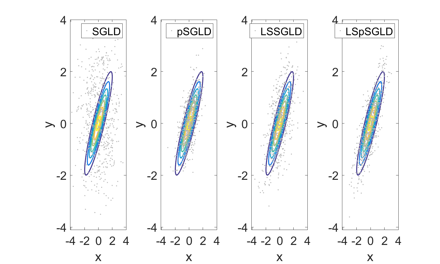
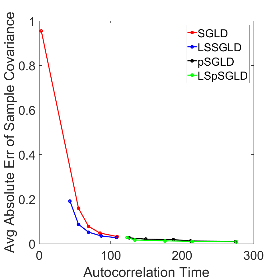
(a) Samples	(b) Error v.s. ACT
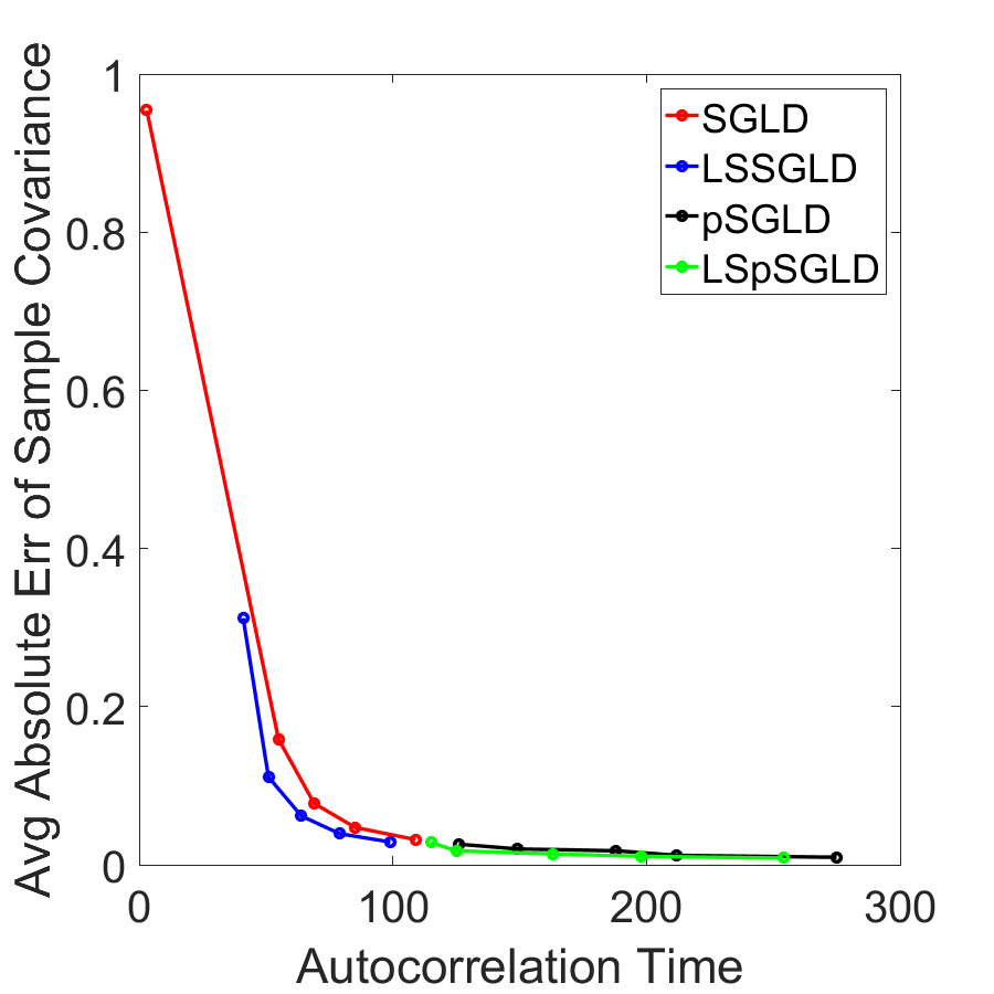
(c) Samples	(d) Error v.s. ACT

Figure 1: Contrasting sampling of a 2D Gaussian distribution with covariance matrix $\Sigma$, with $\Sigma_{11}=\Sigma_{22}=1$ and $\Sigma_{12}=\Sigma_{21}=0.9$, using different samplers. (a) and (c): the first $600$ samples draw by SGLD, pSGLD. (b) and (d): LS-SGLD, and LS-pSGLD. In (c) and (d), we multiply the step size for LS-SGLD and LS-pSGLD by a factor $(1+4\sigma)^{1/4}$.

4.1.2 2D Gaussian Mixture Distribution

In this subsection, we compare the performance of SGLD, pSGLD, LS-SGLD and LS-pSGLD on a Gaussian mixture distribution. In particular, we consider the target distribution

$$\pi\propto\exp{\left(-f({\bm{x}})\right)}=\exp{\left(-\frac{1}{n}\sum_{i=1}^{n}f_{i}({\bm{x}})\right)},\ \ n=500,$$

where each component $\exp{\left(-f_{i}({\bm{x}})\right)}$ is defined as

$$\exp{\left(-f_{i}({\bm{x}})\right)}=\frac{2}{3}e^{-\frac{\|{\bm{x}}-{\bm{a}}_{i}\|_{2}^{2}}{2}}+\frac{1}{3}e^{-\frac{\|{\bm{x}}+{\bm{a}}_{i}\|_{2}^{2}}{2}},$$

where we sample ${\bm{a}}_{i}$ by the MCMC sampler with MH correction from the following 2D Gaussian distribution

$$\mathcal{N}\left(\begin{bmatrix}2\\ 2\end{bmatrix},\begin{bmatrix}2&0\\ 0&2\end{bmatrix}\right).$$

The function $f_{i}({\bm{x}})$ and its gradient can be simplified as

$$f_{i}({\bm{x}})=\frac{\|{\bm{x}}-{\bm{a}}_{i}\|_{2}^{2}}{2}-\log\left(\frac{2}{3}+\frac{1}{3}\exp{\left(-2\langle{\bm{a}}_{i},{\bm{x}}\rangle\right)}\right),$$

$$\nabla f_{i}({\bm{x}})={\bm{x}}-{\bm{a}}_{i}+\frac{2{\bm{a}}_{i}}{2+\exp\left(2\langle{\bm{x}},{\bm{a}}_{i}\rangle\right)}.$$

It can be easily verified that if ${\bm{a}}_{i}$ satisfies $\|{\bm{a}}_{i}\|_{2}>3/2$, the function $f_{i}({\bm{x}})$ defined above is nonconvex. Moreover, it can be seen that

$$\langle\nabla f_{i}({\bm{x}}),{\bm{x}}\rangle=\|{\bm{x}}\|_{2}^{2}-\frac{\exp\left(2\langle{\bm{x}},{\bm{a}}_{i}\rangle\right)}{2+\exp\left(2\langle{\bm{x}},{\bm{a}}_{i}\rangle\right)}\langle{\bm{a}}_{i},{\bm{x}}\rangle\geq\frac{1}{2}\|{\bm{x}}\|_{2}^{2}-\frac{1}{2}\|{\bm{a}}_{i}\|_{2}^{2},$$

which suggests that the function $f_{i}({\bm{x}})$ satisfies the Dissipative Assumption 1 with $m=\frac{1}{2}$ and $b=\frac{\|{\bm{a}}_{i}\|_{2}^{2}}{2}$, and it further implies that $f({\bm{x}})$ is also dissipative.

Since it takes a large number of samples to characterize the distribution, which makes repeated experiments computationally expensive, we instead follow Bardenet et al. (2017); Zou et al. (2019a, b) to use iterates along one Markov chain to visualize the distribution of iterates obtained by MCMC algorithms. We run the four samplers with different numbers of iteration where we set the batch size to be $10$. We plot the distributions generated by different samplers with different numbers of iterations in Fig. 2. As shown in Fig. 2 (c), (f), and (u), when the number of iterations is large enough, e.g. $10^{6}$, the sample distributions of all the three samplers matches well with the reference distribution (sampled by ground-truth sampler, e.g., MCMC with MH step). However, when the number of iterations is not enough, there is a large discrepancy between the sample and target distributions, as shown in Fig. 2 (a), (d), and (g). With a moderate number of iterations, say $5\times 10^{5}$, the sample distribution from LS-SGLD is better than the other two (Fig. 2 (b), (e), and (d)).

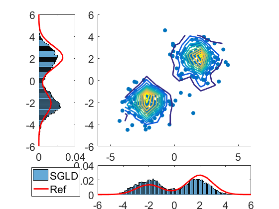
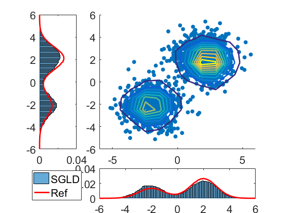
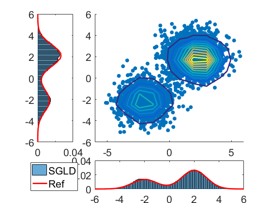
(a) SGLD (1E5)	(b) SGLD (5E5)	(c) SGLD (1E6)
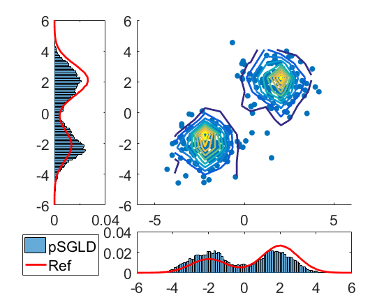
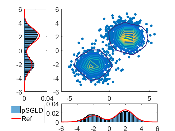
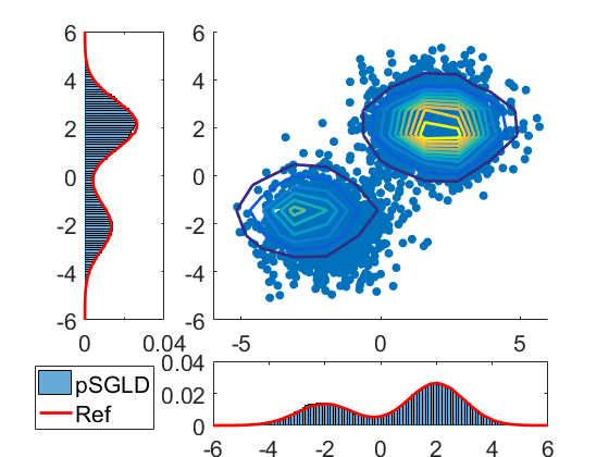
(d) pSGLD (1E5)	(e) pSGLD (5E5)	(f) pSGLD (1E6)
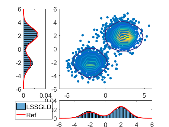
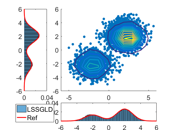
(g) LS-SGLD (1E5)	(h) LS-SGLD (5E5)	(i) LS-SGLD (1E6)

Figure 2: Kernel density plots of samples generated from Gaussian mixture distribution using SGLD, LS-SGLD, pSGLD and LS-pSGLD. We set $\sigma=1.0$ for LS-SGLD and LS-pSGLD.

Let us further evaluate the sample quality in a quantitative approach. We first apply the MCMC with MH step to sample $10K$ samples from the above target distribution. Then we apply SGLD, pSGLD, and LS-SGLD to sample different numbers of samples, respectively, from the target distribution. We measure the 2-Wasserstein distance between the last $10K$ samples of the different number of samples by the above three stochastic gradient samplers with the MH samples. We list the Wasserstein distance between the last $10K$ samples of different numbers of samples from different samplers with the MH samples in Table 2. These results show that the samples generated by LS-SGLD are consistently closer to the samples from MCMC with MH correction.

Table 2: 2-Wasserstein distance between samples sampled by MCMC with Metropolis–Hastings correction and different stochastic gradient Langevin dynamics.

# of Samples	1E5	5E5	9E5
SGLD	0.695	6.726	0.285
pSGLD	5.364	0.286	6.728
LS-SGLD	0.421	0.414	0.418

4.1.3 Comparison of the mixing time between LD and LS-LD

To verify that Laplacian smoothing does not slow down the mixing rate of the continuous-time Markov process, we conduct the following experiments. First, we apply the MCMC with Metropolis-Hasting correction step to sample $10$K points, respectively, from the following two distributions.

• Gaussian distribution with the following probability density function

  $$p(x,y)=\frac{1}{9\pi}\exp{\left(-\left(\frac{(x-1)^{2}}{3^{2}}+\frac{(y-2)^{2}}{3^{2}}\right)\right)}.$$ (17)

• The Gaussian mixture distribution described in subsection 4.1.2.

Second, we use either LD or LS-LD (which can be approximated by Euler-Maruyama discretization with very small step size), to draw samples from the above two distributions and use these samples to estimate the mean of the target densities. Figure 3 plots the MSE between the true and reconstructed (from a different number of samples) means, and they show that LD and LS-LD perform similarly in reconstructing the mean of the target densities.

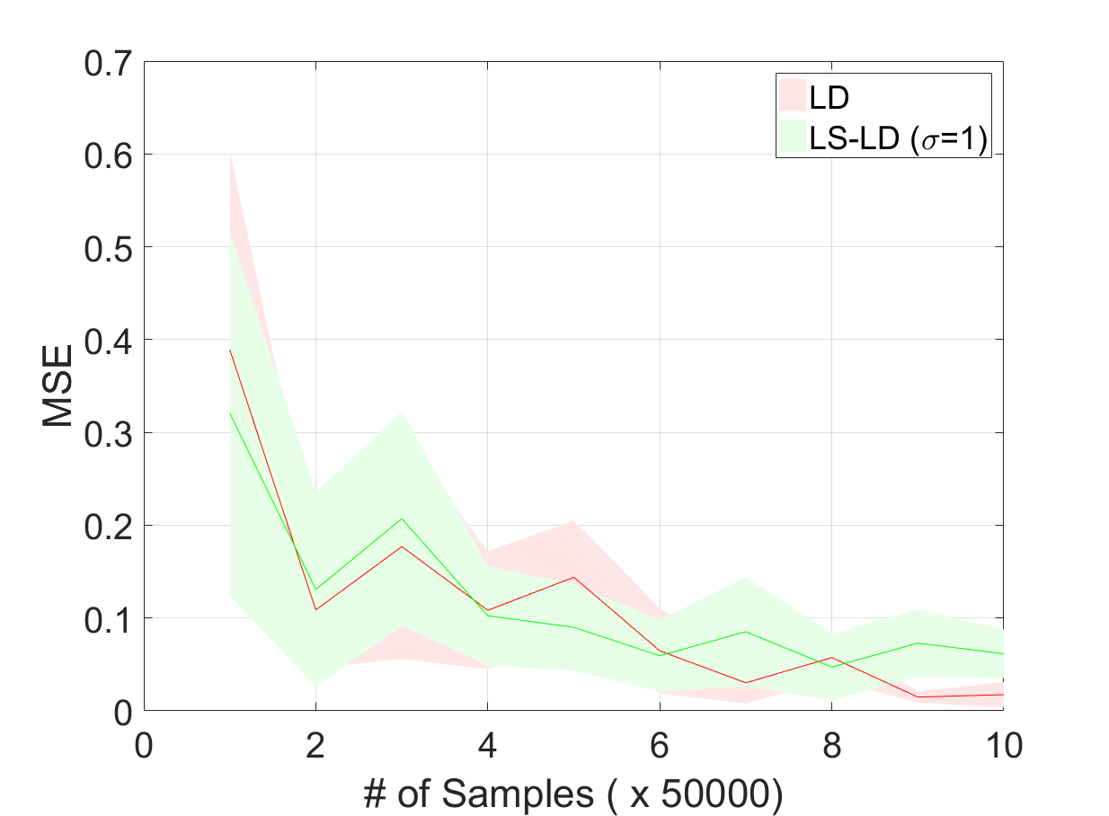
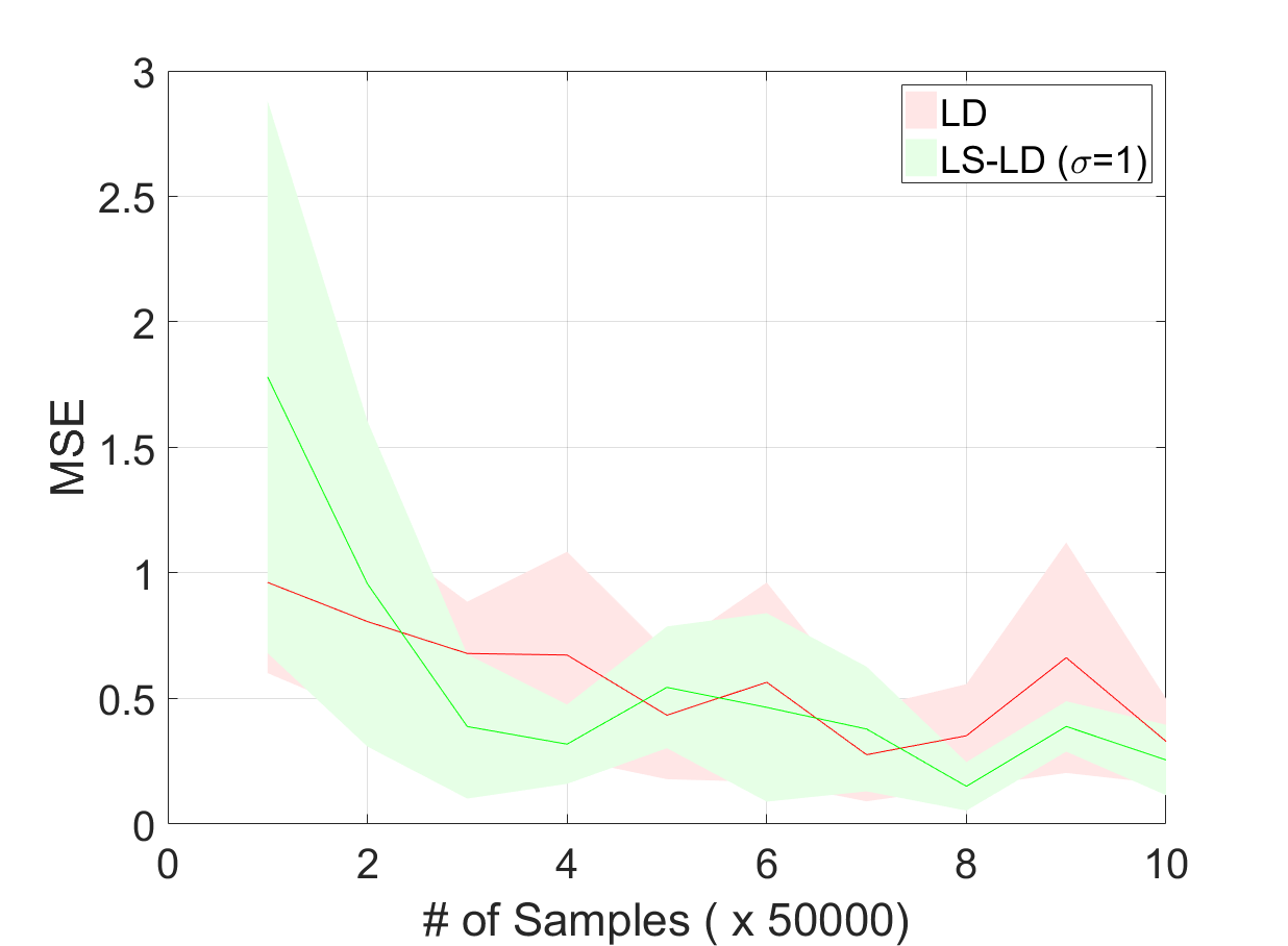
Figure 3: MSE between the true and reconstructed means from different numbers of samples generated by LD and LS-LD (10 independent runs).

4.2 Bayesian Logistic Regression

Suppose we observe $n$ i.i.d samples $\{{\bm{d}}_{i},y_{i}\}_{i=1,2,\cdots,n}$ where ${\bm{d}}_{i}\in{\mathbb{R}}^{d}$ and $y_{i}\in\{-1,1\}$ denote the feature and the corresponding label of the $i$-th sample instance. The likelihood of BLR model is given by

$$p(y_{i}|{\bm{d}}_{i},{\bm{x}})=\frac{1}{1+\exp{\left(-y_{i}\langle{\bm{d}}_{i},{\bm{x}}\rangle\right)}}$$

where ${\bm{x}}$ is the parameter to be learned. We use a Gamma prior $p({\bm{x}})\propto\|{\bm{x}}\|_{2}^{-\lambda}\exp{\left(-\theta\|{\bm{x}}\|_{2}\right)}$ with $\lambda=1$ and $\theta=10^{-2}$. Then we formulate the logarithmic posterior distribution as follows

$$\log\left[p({\bm{x}}|{\bm{d}}_{1},{\bm{d}}_{2},\cdots,{\bm{d}}_{n};y_{1},y_{2},\cdots,y_{n})\right]\propto-\frac{1}{n}\sum_{i=1}^{n}f_{i}({\bm{x}}),$$

where $f_{i}({\bm{x}})=n\log\left(1+e^{-y_{i}\langle{\bm{d}}_{i},{\bm{x}}\rangle}\right)+\lambda\log\left(\|{\bm{x}}\|_{2}\right)+\theta\|{\bm{x}}\|_{2}$.

We use SGLD, pSGLD, LS-SGLD, and LS-pSGLD with batch size $5$ to train a Bayesian logistic regression (BLR) model on the benchmark a3a dataset from the UCI machine learning repository . The a3a dataset contains $3185$ training data and $29376$ test instances, each data instance is of dimension $122$. We use the grid search to determine the optimal learning rate for SGLD ($0.001$) and pSGLD ($0.002$), and then we multiply them by $(1+4\sigma)^{1/4}$ to get the learning rate for LS-SGLD and LS-pSGLD. We set the burn-in to be $1000$ for all these four samplers. After burn-in, we compute the moving average of the sample parameters to estimate the regression parameters ${\bm{x}}$. We plot iteration v.s. negative log-likelihood and accuracy in Fig. 4, and we see that Laplacian smoothing reduces the negative log-likelihood and increases the accuracy. The preconditioning accelerates mixing initially, however, the gap between sampling and target distribution is remarkably larger than the case without preconditioning.

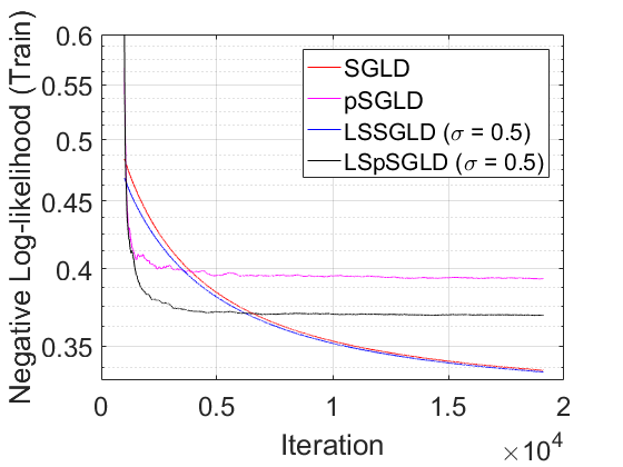
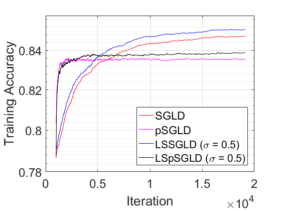
(a) Log-likelihood (Training Set)	(b) Training Accuracy
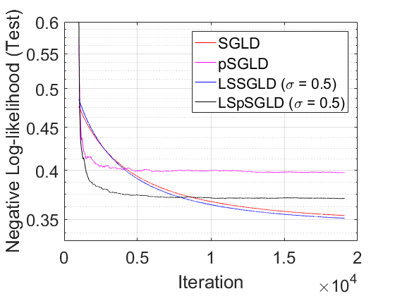
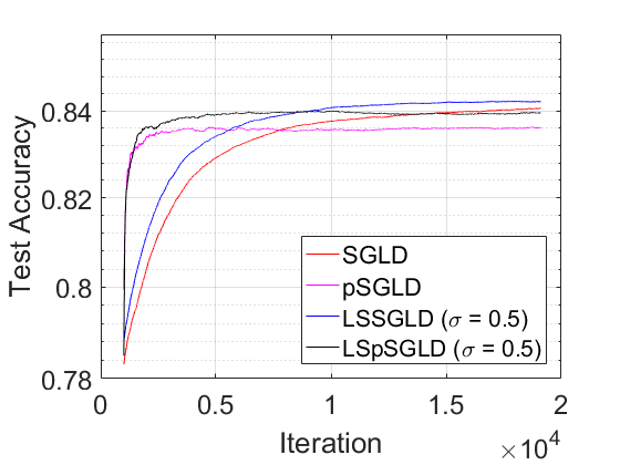
(c) Log-likelihood (Test Set)	(d) Test Accuracy

Figure 4: Convergence comparison for Bayesian logistic regression, where the X-axis represents the number of iterations and Y-axis represents the negative log-likelihood/accuracy. (a) Negative log-likelihood on training dataset; (b) Accuracy on training dataset; (c) Negative log-likelihood on test dataset; (d) Accuracy on test dataset.

4.2.1 Variance reduction in stochastic gradient

We numerically verify the efficiency of variance reduction on BLR for a3a dataset classification. We first compute a path by full batch SGLD with the same learning rate as before, and meanwhile, we record the Laplacian smoothing gradient on each point along the path. Then we compute the Laplacian smoothing stochastic gradients on each point along the path by using different batch size and $\sigma$. We run 100 independent experiments to acquire the Laplacian smoothing stochastic gradients, and then we compute the variance of these stochastic gradients by regarding the full batch Laplacian smoothing gradient as the mean. In Table 3, we report the maximum variance, among all coordinates of the gradient and all points on the descent path, for each pair of batch size and $\sigma$.

Table 3: The maximum variance of the stochastic gradients generated by LS-SGLD on training BLR on the a3a data. $\sigma=0$ reduces to SGLD.

Batch Size	10	15	50
$\sigma=0$	7.69E-1	3.17E-1	5.69E-2
$\sigma=0.5$	2.56E-1	1.06E-2	1.96E-2
$\sigma=1.0$	1.54E-1	6.37E-2	1.21E-2
$\sigma=2.0$	8.52E-2	3.54E-2	7.04E-3

4.3 Bayesian Convolutional Neural Network

We consider training a CNN by SGLD, pSGLD, LS-SGLD, and LS-pSGLD on the MNIST benchmark with batch size $100$, the architecture of the CNN is

$$\mbox{CNN:}\ {\rm input}_{28\times 28}\rightarrow{\rm conv}_{20,5,2}\rightarrow{\rm conv}_{20,20,5}\rightarrow{\rm fc}_{128}\rightarrow{\rm softmax}.$$

The notation ${\rm conv}_{c,k,m}$ denotes a 2D convolutional layer with $c$ output channels, each of which is the sum of a channel-wise convolution operation on the input using a learnable kernel of size $k\times k$, it further adds ReLU nonlinearity and max-pooling with stride size $m$. ${\rm fc}_{128}$ is an affine transformation that transforms the input to a vector of dimension $128$. Finally, the tensors are activated by a multi-class logistic function.

Similar to BLR, we use a Gamma prior $p({\bm{x}})\propto\|{\bm{x}}\|_{2}^{-\lambda}\exp{\left(-\theta\|{\bm{x}}\|_{2}\right)}$ with $\lambda=1$ and $\theta=5e^{-4}$. Again, we use the grid search to find the optimal step size for SGLD and pSGLD which is $0.02$ and $2e-4$, respectively. We multiply the optimal step size for SGLD and pSGLD by a factor $(1+4\sigma)^{1/4}$ to get the step size for LS-SGLD and LS-pSGLD, and we let $\sigma=0.5$ for Laplacian smoothing. The comparisons between different sampling algorithms are plotted in Fig. 5, we see that Laplacian smoothing reduces the negative log-likelihood and increases the accuracy of both training and test datasets. The preconditioning accelerates mixing and reduces the gap between sampling and target distribution. Here, we applied early stopping in training CNN by pSGLD and LS-pSGLD.

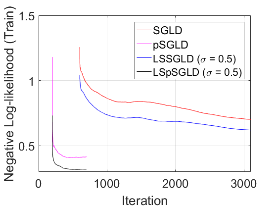
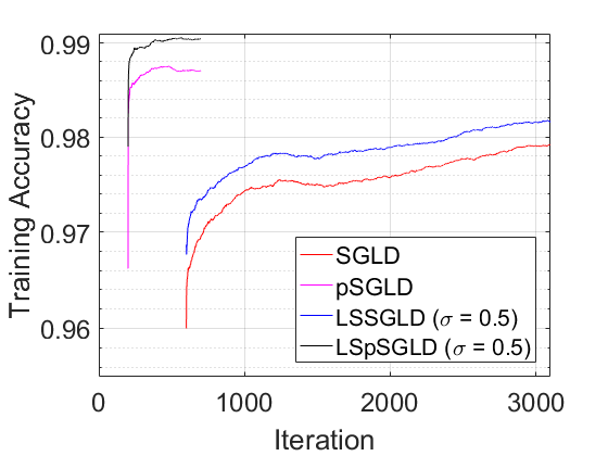
(a) Log-likelihood (Training Set)	(b) Training Accuracy
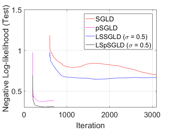
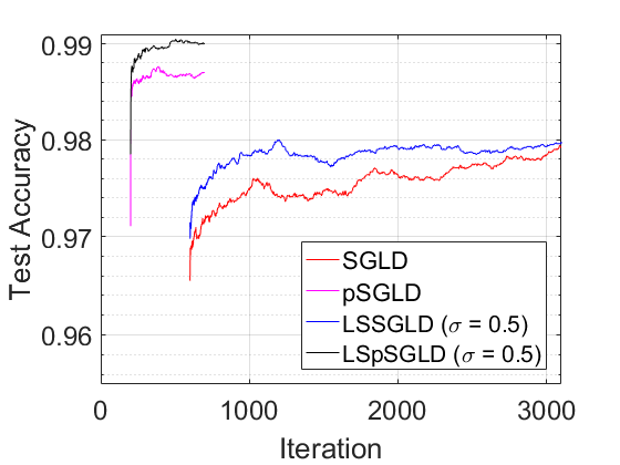
(c) Log-likelihood (Test Set)	(d) Test Accuracy

Figure 5: Convergence comparison for Bayesian convolutional neural network, where the X-axis represents the number of iterations and Y-axis represents the negative log-likelihood/accuracy. (a) Negative log-likelihood on training dataset; (b) Accuracy on training dataset; (c) Negative log-likelihood on test dataset; (d) Accuracy on test dataset.

5 Conclusions

In this paper, we integrate Laplacian smoothing with Stochastic Gradient Langevin Dynamics (SGLD) to reduce the gap between the sample and target distributions. The resulting algorithm also allows us to take a larger step size. The proposed algorithm is simple to implement and the extra computation and memory costs compared with the SGLD are negligible when the Fast Fourier Transform (FFT)-based algorithms is employed to resolve the dynamics of the resulting Laplacian Smoothing SGLD (LS-SGLD). We show, both theoretically and empirically, that LS-SGLD can improve the sample quality. It is straightforward to extend Laplacian smoothing to the other Markov Chain Monte Carlo (MCMC) algorithms, e.g., the stochastic gradient Hamiltonian Monte Carlo (Chen et al., 2014).

Appendix A Missing proof in Section 2

In this section, we provide the proof of Proposition 1.

Proof of Proposition 1 .

Let $p({\bm{x}},t)$ be the distribution of ${\bm{X}}_{t}$. Then we know that $p({\bm{x}},t)$ satisfies the following Fokker-Planck equation

$$\frac{\partial p({\bm{x}},t)}{\partial t} =\frac{1}{\beta}\langle{\mathbf{A}}_{\sigma}^{-1},\nabla^{2}p({\bm{x}},t)\rangle+\langle\nabla,p({\bm{x}},t){\mathbf{A}}_{\sigma}^{-1}\nabla f({\bm{x}})\rangle$$

$$=\frac{1}{\beta}\langle\nabla,{\mathbf{A}}_{\sigma}^{-1}\nabla p({\bm{x}},t)\rangle+\langle\nabla,p({\bm{x}},t){\mathbf{A}}_{\sigma}^{-1}\nabla f({\bm{x}})\rangle,$$ (18)

where $\langle\nabla,\mathbf{h}({\bm{x}})\rangle$ denotes the divergence of the vector field $\mathbf{h}({\bm{x}})$. Since the stationary distribution $\pi$ satisfies $\partial\pi/\partial t=0$, we have

$$\frac{1}{\beta}\langle\nabla,{\mathbf{A}}_{\sigma}^{-1}\nabla p({\bm{x}},t)\rangle+\langle\nabla,p({\bm{x}},t){\mathbf{A}}_{\sigma}^{-1}\nabla f({\bm{x}})\rangle=0,$$

which further implies that $\beta^{-1}\nabla\pi+\pi\nabla f({\bm{x}})=0$. Solving this equation directly gives $\pi\propto e^{-\beta f({\bm{x}})}$, which completes the proof.

∎

Appendix B Proof of Main Theory

In order to bound sampling error between the distribution of the output of LS-SGLD and the target distribution $\pi\propto e^{-\beta f({\bm{x}})}$, we consider a reference sequence generated by LS-LD (6), denoted by $\{{\bm{X}}_{t}\}_{t\geq 0}$. Let ${\bm{X}}_{0}={\bm{x}}_{0}$, by triangle inequality, we can decompose the $2$-Wasserstein distance ${\mathcal{W}}_{2}({\mathbb{P}}({\bm{x}}_{K}),\pi)$ as follows

$${\mathcal{W}}_{2}({\mathbb{P}}({\bm{x}}_{K}),\pi)\leq{\mathcal{W}}_{2}({\mathbb{P}}({\bm{x}}_{K}),{\mathbb{P}}({\bm{X}}_{K\eta}))+{\mathcal{W}}_{2}({\mathbb{P}}({\bm{X}}_{K\eta}),\pi).$$

The first term on the R.H.S. stands for the discretization error of the numerical integrator, and the second term denotes the ergodicity of LS-LD (6), which characterizes the mixing time of LS-LD. In what follows, we first deliver the following lemma that characterizes the error term ${\mathcal{W}}_{2}({\mathbb{P}}({\bm{X}}_{K\eta}),\pi)$.

Lemma 5.

Under Assumptions 1 and 2, there exists a constant $c_{0}\in[\|{\mathbf{A}}_{\sigma}\|_{2}^{-1},1]$

$${\mathcal{W}}_{2}\big{(}{\mathbb{P}}({\bm{X}}_{K\eta}),\pi\big{)}\leq\big{[}2\lambda\big{(}\beta f(0)+\log(\Lambda)\big{)}\big{]}^{1/2}\cdot e^{-c_{0}K\eta/(2\beta\lambda)},$$

where $\Lambda=\int_{{\mathbb{R}}^{d}}e^{-\beta f({\bm{x}})}\text{d}{\bm{x}}$ and $\lambda$ denotes the logarithmic Sobolev constant of the target distribution $\pi\propto e^{-\beta f({\bm{x}})}$.

Note that Lemma 5 does not require that the target density is log-concave, which can be utilized to prove the convergence rate of LS-SGLD for sampling both log-concave and non-log-concave densities. In the following, we are going to complete the proofs of Theorems 1 and 2.

B.1 Proof of Theorem 1

We first provide the following lemma which proves an upper bound of the discretization error ${\mathcal{W}}_{2}\big{(}{\mathbb{P}}({\bm{x}}_{K}),P({\bm{X}}_{K\eta})\big{)}$ for sampling log-concave densities.

Lemma 6.

Under Assumptions 1, 2, 3 and 4, if set the step size $\eta\leq Cm\beta^{-1}/M^{2}$ for some sufficiently small constant $C$, there exist constants $\gamma_{1}\in[\|{\mathbf{A}}_{\sigma}\|_{2}^{-2},1]$ and $\gamma_{2}=d^{-1}\sum_{i=1}^{d}(1+2\sigma-2\sigma\cos(2\pi i/d))^{-1}$ such that the following holds

$${\mathcal{W}}_{2}\big{(}{\mathbb{P}}({\bm{x}}_{K}),P({\bm{X}}_{K\eta})\big{)}\leq\bigg{(}\frac{2\gamma_{1}d\omega^{2}K\eta^{2}}{B}\bigg{)}^{1/2}+\big{[}8\gamma_{2}K(K+1)\beta^{-1}d\eta^{3}\big{]}^{1/2}$$

Then we can complete the proof of Theorem 1 as follows.

Proof of Theorem 1.

By triangle inequality and Lemmas 5 and 6, it is evident that

$${\mathcal{W}}_{2}({\mathbb{P}}({\bm{x}}_{K}),\pi) \leq{\mathcal{W}}_{2}({\mathbb{P}}({\bm{x}}_{K}),{\mathbb{P}}({\bm{X}}_{K\eta}))+{\mathcal{W}}_{2}({\mathbb{P}}({\bm{X}}_{K\eta}),\pi)$$

$$\leq\bigg{(}\frac{2\gamma_{1}d\omega^{2}K\eta^{2}}{B}\bigg{)}^{1/2}+\big{[}8\gamma_{2}K(K+1)\beta^{-1}d\eta^{3}\big{]}^{1/2}+\big{[}2\lambda\big{(}\beta f(0)+\log(\Lambda)\big{)}\big{]}^{1/2}\cdot e^{-c_{0}K\eta/(2\beta\lambda)},$$

which completes the proof.

∎

B.2 Proof of Theorem 2

Similar to the proof of Theorem 1, we provide the following lemma that characterizes the discretization error ${\mathcal{W}}_{2}\big{(}{\mathbb{P}}({\bm{x}}_{k}),{\mathbb{P}}({\bm{X}}_{k\eta})\big{)}$ for sampling from non-log-concave densities.

Lemma 7.

Under Assumptions 1 and 2, if set the step size $\eta\leq Cm\beta^{-1}/M^{2}$ for some sufficiently small constant $C$, there exist constants $\gamma_{1}\in[\|{\mathbf{A}}_{\sigma}\|_{2}^{-2},1]$, $\gamma_{2}=d^{-1}\sum_{i=1}^{d}(1+2\sigma-2\sigma\cos(2\pi i/d))^{-1}$ and $\bar{\Gamma}=\big{(}3/2+2(b+\beta^{-1}d)\big{)}^{1/2}$ such that the following holds,

$${\mathcal{W}}_{2}\big{(}{\mathbb{P}}({\bm{x}}_{K}),{\mathbb{P}}({\bm{X}}_{K\eta})\big{)}\leq\bar{\Gamma}(K\eta)^{1/2}\bigg{[}\bigg{(}\frac{\gamma_{1}\beta d\omega^{2}}{2B}K\eta+2\gamma_{2}\beta M^{2}dK\eta^{2}\bigg{)}^{1/2}+\bigg{(}\frac{\gamma_{1}\beta d\omega^{2}}{2B}K\eta+2\gamma_{2}\beta M^{2}dK\eta^{2}\bigg{)}^{1/4}\bigg{]}.$$

Proof of Theorem 2.

By triangle inequality and Lemmas 5 and 7, it is evident that

$${\mathcal{W}}_{2}({\mathbb{P}}({\bm{x}}_{K}),\pi) \leq{\mathcal{W}}_{2}({\mathbb{P}}({\bm{x}}_{K}),{\mathbb{P}}({\bm{X}}_{K\eta}))+{\mathcal{W}}_{2}({\mathbb{P}}({\bm{X}}_{K\eta}),\pi)$$

$$\leq\bar{\Gamma}(K\eta)^{1/2}\bigg{[}\bigg{(}\frac{\gamma_{1}\beta d\omega^{2}}{2B}K\eta+2\gamma_{2}M^{2}dK\eta^{2}\bigg{)}^{1/2}+\bigg{(}\frac{\gamma_{1}\beta d\omega^{2}}{2B}K\eta+2\gamma_{2}M^{2}dK\eta^{2}\bigg{)}^{1/4}\bigg{]}$$

$$\quad+\big{[}2\lambda\big{(}\beta f(0)+\log(\Lambda)\big{)}\big{]}^{1/2}\cdot e^{-c_{0}K\eta/(2\beta\lambda)},$$

which completes the proof.

∎

Appendix C Proof of lemmas in Appendix B

C.1 Proof of Lemma 5

In order to prove Lemma 5, we require the following lemma.

Lemma 8 (Theorem 9.6.1 in Bakry et al. (2013)).

Suppose the target density $\pi$ satisfies logarithmic Sobolev inequality with a positive constant $\lambda$, for any density $\mu$ it holds that

$${\mathcal{W}}_{2}(\mu,\pi)\leq\sqrt{2\lambda D_{KL}(\mu||\pi)}.$$

Proof of Lemma 5.

Recall that for LS-LD (6), the distribution of ${\bm{X}}_{t}$, denoted by $p({\bm{x}},t)$, can be described by the following Fokker-Planck equation

$$\frac{\partial p({\bm{x}},t)}{\partial t} =\frac{1}{\beta}\langle{\mathbf{A}}_{\sigma}^{-1},\nabla^{2}p({\bm{x}},t)\rangle+\langle\nabla,p({\bm{x}},t){\mathbf{A}}_{\sigma}^{-1}\nabla f({\bm{x}})\rangle$$

$$=\frac{1}{\beta}\langle\nabla,{\mathbf{A}}_{\sigma}^{-1}\nabla p({\bm{x}},t)\rangle+\langle\nabla,p({\bm{x}},t){\mathbf{A}}_{\sigma}^{-1}\nabla f({\bm{x}})\rangle,$$ (19)

where $\langle\nabla,\mathbf{h}({\bm{x}})\rangle$ denotes the divergence of the vector field $\mathbf{h}({\bm{x}})$. Let ${\mathbb{P}}_{t}$ be the short-hand notation of $p({\bm{x}},t)$, and denote by $D_{KL}({\mathbb{P}}_{t}||\pi)$ the KL-divergence between the distribution ${\mathbb{P}}_{t}$ and the target distribution $\pi$. Then, we have

$$\frac{\text{d}D_{KL}({\mathbb{P}}_{t}||\pi)}{\text{d}t} =\int_{{\mathbb{R}}^{d}}\frac{\partial}{\partial t}\bigg{[}{\mathbb{P}}_{t}\log\bigg{(}\frac{{\mathbb{P}}_{t}}{\pi}\bigg{)}\bigg{]}\text{d}{\bm{x}}$$

$$=\int_{{\mathbb{R}}^{d}}\frac{\partial{\mathbb{P}}_{t}}{\partial t}\big{[}\log({\mathbb{P}}_{t})+1-\log(\pi)\big{]}\text{d}{\bm{x}}.$$

Similar to the proof of Proposition 2 in Mou et al. (2017), by (C.1) we further have

$$\frac{\text{d}D_{KL}({\mathbb{P}}_{t}||\pi)}{\text{d}t} =-\int_{{\mathbb{R}}^{d}}\bigg{\langle}\frac{1}{\beta}{\mathbf{A}}_{\sigma}^{-1}\nabla{\mathbb{P}}_{t}+{\mathbb{P}}_{t}{\mathbf{A}}_{\sigma}^{-1}\nabla f({\bm{x}}),\nabla\log({\mathbb{P}}_{t})-\nabla\log(\pi)\bigg{\rangle}\text{d}{\bm{x}}$$

$$=-\int_{{\mathbb{R}}^{d}}\bigg{\langle}{\mathbf{A}}_{\sigma}^{-1}\bigg{(}\frac{1}{\beta}{\mathbb{P}}_{t}\nabla\log({\mathbb{P}}_{t})+{\mathbb{P}}_{t}\nabla f({\bm{x}})\bigg{)},\nabla\log({\mathbb{P}}_{t})-\nabla\log(\pi)\bigg{\rangle}\text{d}{\bm{x}},$$

where the second equality holds due to $\nabla{\mathbb{P}}_{t}={\mathbb{P}}_{t}\nabla\log({\mathbb{P}}_{t})$. In addition, note that $\pi\propto e^{-\beta f({\bm{x}})}$, we have $\nabla\log(\pi)=-\beta\nabla f({\bm{x}})$. Then we have

$$\frac{\text{d}D_{KL}({\mathbb{P}}_{t}||\pi)}{\text{d}t} =-\frac{1}{\beta}\int_{{\mathbb{R}}_{d}}\big{\langle}{\mathbf{A}}_{\sigma}^{-1}\big{(}\nabla\log({\mathbb{P}}_{t})-\nabla\log(\pi)\big{)},\nabla\log({\mathbb{P}}_{t})-\nabla\log(\pi)\big{\rangle}{\mathbb{P}}_{t}\text{d}{\bm{x}}$$

$$=-\frac{1}{\beta}\int_{{\mathbb{R}}_{d}}\|\nabla\log({\mathbb{P}}_{t})-\nabla\log(\pi)\|_{{\mathbf{A}}_{\sigma}^{-1}}^{2}{\mathbb{P}}_{t}\text{d}{\bm{x}}.$$

Since ${\mathbf{A}}_{\sigma}$ is a positive definite matrix, there exists a constant $c_{0}\in[\|{\mathbf{A}}_{\sigma}\|_{2}^{-1},1]$ such that

$$\frac{\text{d}D_{KL}({\mathbb{P}}_{t}||\pi)}{\text{d}t}\leq-\frac{c_{0}}{\beta}\int_{{\mathbb{R}}_{d}}\|\nabla\log({\mathbb{P}}_{t})-\nabla\log(\pi)\|_{2}^{2}{\mathbb{P}}_{t}\text{d}{\bm{x}}=-\frac{c_{0}}{\beta}{\mathbf{I}}({\mathbb{P}}_{t}||\pi),$$ (20)

where ${\mathbf{I}}({\mathbb{P}}_{t}||\pi)$ denotes the fisher information between ${\mathbb{P}}_{t}$ and $\pi$. By Proposition 2, we know that the target density $\pi$ satisfies logarithmic Sobolev inequality with constant $\lambda>0$. Then, from Markowich and Villani (1999), we have

$$D_{KL}({\mathbb{P}}_{t}||\pi)\leq\frac{1}{\lambda}{\mathbf{I}}({\mathbb{P}}_{t}||\pi).$$

Plugging the above inequality into (20), we obtain

$$\frac{\text{d}D_{KL}({\mathbb{P}}_{t}||\pi)}{\text{d}t}\leq-\frac{c_{0}}{\lambda\beta}D_{KL}({\mathbb{P}}_{t}||\pi),$$

which implies that

$$D_{KL}({\mathbb{P}}_{t}||\pi)\leq D_{KL}({\mathbb{P}}_{0}||\pi)e^{-c_{0}t/(\beta\lambda)}.$$

Note that we have ${\mathbb{P}}_{0}=\delta(0)$, where $\delta(\cdot)$ is the Dirac delta function, thus,

$$D_{KL}({\mathbb{P}}_{0}||\pi)=\int_{{\mathbb{R}}^{d}}{\mathbb{P}}_{0}\big{[}\log({\mathbb{P}}_{0})-\log(\pi)\big{]}\text{d}{\bm{x}}=-\log(\pi)|_{{\bm{x}}=0}=\beta f(0)+\log(\Lambda),$$

where $\Lambda=\int_{{\mathbb{R}}^{d}}e^{-\beta f({\bm{x}})}\text{d}{\bm{x}}$. Then by Lemma 8, we have the following regarding the $2$-Wasserstein distance ${\mathcal{W}}_{2}\big{(}{\mathbb{P}}({\bm{X}}_{k\eta}),\pi\big{)}$,

$${\mathcal{W}}_{2}\big{(}{\mathbb{P}}({\bm{X}}_{k\eta}),\pi\big{)}\leq\sqrt{2\lambda D_{KL}({\mathbb{P}}({\bm{X}}_{0})||\pi)}\cdot e^{-c_{0}t/(2\beta\lambda)}=\big{[}2\lambda\big{(}\beta f(0)+\log(\Lambda)\big{)}\big{]}^{1/2}\cdot e^{-c_{0}t/(2\beta\lambda)},$$

which completes the proof. ∎

C.2 Proof of Lemma 6

We first deliver the following useful lemmas.

Lemma 9.

Consider any two LS-LD sequences $\{{\bm{W}}_{t}\}_{t\geq 0}$ and $\{{\bm{V}}_{t}\}_{t\geq 0}$, and assume that ${\bm{W}}_{t}$ and ${\bm{V}}_{t}$ have shared Brownian motion terms. Under Assumption 4, for any $t>0$ it holds that,

$${\mathbb{E}}[\|{\bm{W}}_{t}-{\bm{V}}_{t}\|_{{\mathbf{A}}_{\sigma}}^{2}]\leq{\mathbb{E}}[\|{\bm{W}}_{0}-{\bm{V}}_{0}\|_{{\mathbf{A}}_{\sigma}}^{2}].$$

Lemma 10.

Under Assumptions 1 and 2, if set the step size $\eta\leq Cm\beta^{-1}/M^{2}$ for some sufficiently small constant $C$, there exists a constant $\gamma_{2}=d^{-1}\sum_{i=1}^{d}(1+2\sigma-2\sigma\cos(2\pi i/d))^{-1}$ such that for any ${\bm{x}}_{k}$ with $k\geq 0$,

$${\mathbb{E}}[\|{\mathcal{L}}_{\eta}{\bm{x}}_{k}-{\mathcal{G}}_{\eta}{\bm{x}}_{k}\|_{{\mathbf{A}}_{\sigma}}^{2}]\leq 4\gamma_{2}\beta^{-1}d\eta^{3}.$$

Now we are ready to complete the proof of Lemma 6.

Proof of Lemma 6.

For the sake of simplicity, we first define three operators ${\mathcal{L}}_{t}$, ${\mathcal{G}}_{t}$ and ${\mathcal{S}}_{t}$ as follows: for any ${\bm{x}}\in{\mathbb{R}}^{d}$ we denote by ${\mathcal{L}}_{t}{\bm{x}}$ the random point generated by LS-LD at time $t$ starting from ${\bm{x}}$, ${\mathcal{G}}_{t}{\bm{x}}$ the point after performing one-step LS-SGLD with full gradient at ${\bm{x}}$ with step size $t$, and ${\mathcal{S}}_{t}{\bm{x}}$ the point after performing one-step LS-SGLD at ${\bm{x}}$ with step size $t$. Then we have

$${\mathbb{E}}[\|{\bm{x}}_{K}-{\bm{X}}_{K\eta}\|_{{\mathbf{A}}_{\sigma}}^{2}] ={\mathbb{E}}[\|{\bm{x}}_{K}-{\mathcal{G}}_{\eta}{\bm{x}}_{K-1}+{\mathcal{G}}_{\eta}{\bm{x}}_{K-1}-{\bm{X}}_{K\eta}\|_{{\mathbf{A}}_{\sigma}}^{2}]$$

$$={\mathbb{E}}[\|{\bm{x}}_{K}-{\mathcal{G}}_{\eta}{\bm{x}}_{K-1}\|_{{\mathbf{A}}_{\sigma}}^{2}]+{\mathbb{E}}[\|{\mathcal{G}}_{\eta}{\bm{x}}_{K-1}-{\bm{X}}_{K\eta}\|_{{\mathbf{A}}_{\sigma}}^{2}],$$ (21)

where the second equality follows from the fact that ${\mathbb{E}}[\langle{\bm{x}}_{K}-{\mathcal{G}}_{\eta}{\bm{x}}_{K-1},{\mathbf{A}}_{\sigma}({\mathcal{G}}_{\eta}{\bm{x}}_{K-1}-{\bm{X}}_{K\eta})\rangle]=0$ since at any iteration the randomness of stochastic gradient is independent of the iterate. Regarding the first term on the R.H.S. of (C.2), we have

$${\mathbb{E}}[\|{\bm{x}}_{K}-{\mathcal{G}}_{\eta}{\bm{x}}_{K-1}\|_{{\mathbf{A}}_{\sigma}}^{2}] =\eta^{2}{\mathbb{E}}[\|{\mathcal{S}}_{\eta}{\bm{x}}_{K-1}-{\mathcal{G}}_{\eta}{\bm{x}}_{K-1}\|_{{\mathbf{A}}_{\sigma}}^{2}]$$

$$\leq\eta^{2}{\mathbb{E}}[\|{\mathbf{A}}_{\sigma}^{-1}{\mathbf{g}}_{K-1}-{\mathbf{A}}_{\sigma}^{-1}\nabla f({\bm{x}}_{K-1})\|_{{\mathbf{A}}_{\sigma}}^{2}]$$

$$\leq\frac{\eta^{2}}{B}{\mathbb{E}}[\|{\mathbf{A}}_{\sigma}^{-1}\nabla f_{i}({\bm{x}}_{K-1})-{\mathbf{A}}_{\sigma}^{-1}\nabla f({\bm{x}}_{K-1})\|_{{\mathbf{A}}_{\sigma}}^{2}]$$

$$\leq\frac{\gamma_{1}\eta^{2}d\omega^{2}}{B},$$ (22)

where $\gamma_{1}\in[\|{\mathbf{A}}_{\sigma}\|_{2}^{-1},1)$ is a problem-dependent parameter, the first inequality follows the definitions of operators ${\mathcal{S}}_{\eta}$ and ${\mathcal{G}}_{\eta}$, the second inequality follows from Lemma A.1 in Lei et al. (2017) and the last inequality is by Assumption 3. In terms of the second term on the R.H.S. of (C.2), we have

$${\mathbb{E}}[\|{\mathcal{G}}_{\eta}{\bm{x}}_{K-1}-{\bm{X}}_{K\eta}\|_{{\mathbf{A}}_{\sigma}}^{2}] ={\mathbb{E}}[\|{\mathcal{G}}_{\eta}{\bm{x}}_{K-1}-{\mathcal{L}}_{\eta}{\bm{x}}_{K-1}+{\mathcal{L}}_{\eta}{\bm{x}}_{K-1}-{\bm{X}}_{K\eta}\|_{{\mathbf{A}}_{\sigma}}^{2}]$$

$$\leq(1+\alpha){\mathbb{E}}[\|{\mathcal{G}}_{\eta}{\bm{x}}_{K-1}-{\mathcal{L}}_{\eta}{\bm{x}}_{K-1}\|_{{\mathbf{A}}_{\sigma}}^{2}]+(1+1/\alpha){\mathbb{E}}[\|{\mathcal{L}}_{\eta}{\bm{x}}_{K-1}-{\mathcal{L}}_{\eta}{\bm{X}}_{(K-1)\eta}\|_{{\mathbf{A}}_{\sigma}}^{2}]$$

$$\leq 4(1+\alpha)\gamma_{2}\beta^{-1}d\eta^{3}+(1+1/\alpha){\mathbb{E}}[\|{\bm{x}}_{K-1}-{\bm{X}}_{(K-1)\eta}\|_{{\mathbf{A}}_{\sigma}}^{2}],$$ (23)

where $\alpha$ is a positive constant that will be specified later, the first inequality is by Young’s inequality, and the second inequality follows from Lemmas 9 and 10. Plugging (C.2) and (C.2) into (C.2) gives

$${\mathbb{E}}[\|{\bm{x}}_{K}-{\bm{X}}_{K\eta}\|_{{\mathbf{A}}_{\sigma}}^{2}] \leq 4(1+\alpha)\gamma_{2}\beta^{-1}d\eta^{3}+\frac{\gamma_{1}\eta^{2}d\omega^{2}}{B}+(1+1/\alpha){\mathbb{E}}[\|{\bm{x}}_{K-1}-{\bm{X}}_{(K-1)\eta}\|_{{\mathbf{A}}_{\sigma}}^{2}].$$

Then, by recursively applying the above inequality, we obtain

$${\mathbb{E}}[\|{\bm{x}}_{K}-{\bm{X}}_{K\eta}\|_{{\mathbf{A}}_{\sigma}}^{2}] \leq(1+1/\alpha)^{K}{\mathbb{E}}[\|{\bm{x}}_{0}-{\bm{X}}_{0}\|_{{\mathbf{A}}_{\sigma}}^{2}]+\sum_{k=0}^{K-1}(1+1/\alpha)^{k}\bigg{[}4(1+\alpha)\gamma_{2}\beta^{-1}d\eta^{3}+\frac{\gamma_{1}\eta^{2}d\omega^{2}}{B}\bigg{]}$$

$$=\alpha\big{[}(1+1/\alpha)^{K}-1\big{]}\cdot\bigg{[}4(1+\alpha)\gamma_{2}\beta^{-1}d\eta^{3}+\frac{\gamma_{1}\eta^{2}d\omega^{2}}{B}\bigg{]}.$$

Let $\alpha=K$ and apply the inequality $(1+1/K)^{K}-1\leq e-1\leq 2$, the above inequality implies

$${\mathbb{E}}[\|{\bm{x}}_{K}-{\bm{X}}_{K\eta}\|_{{\mathbf{A}}_{\sigma}}^{2}]\leq 2K\eta^{2}\cdot\bigg{[}\frac{\gamma_{1}d\omega^{2}}{B}+4(K+1)\gamma_{2}\beta^{-1}d\eta\bigg{]}.$$

Based on the definition of $2$-Wasserstein distance, we have

$${\mathcal{W}}_{2}^{2}\big{(}{\mathbb{P}}({\bm{x}}_{K}),{\mathbb{P}}({\bm{X}}_{K\eta})\big{)}\leq\sqrt{{\mathbb{E}}[\|{\bm{x}}_{K}-{\bm{X}}_{K\eta}\|_{2}^{2}]}\leq\sqrt{{\mathbb{E}}[\|{\bm{x}}_{K}-{\bm{X}}_{K\eta}\|_{{\mathbf{A}}_{\sigma}}^{2}]}\leq\bigg{(}\frac{2\gamma_{1}d\omega^{2}K\eta^{2}}{B}\bigg{)}^{1/2}+\big{[}8\gamma_{2}K(K+1)\beta^{-1}d\eta^{3}\big{]}^{1/2},$$

where the last inequality is by the fact that $\sqrt{x^{2}+y^{2}}\leq|x|+|y|$. This completes the proof.

∎

C.3 Proof of Lemma 7

In order to prove Lemma 7, we require the following lemmas.

Lemma 11.

Under Assumptions 1 and 2, for all $k\geq 0$, there exists a constant $c_{1}\in[\|{\mathbf{A}}_{\sigma}\|_{2}^{-1},1)$ such that

$${\mathbb{E}}[\|{\bm{x}}_{k}\|_{2}^{2}]\leq{\mathbb{E}}[\|{\bm{x}}_{k}\|_{{\mathbf{A}}_{\sigma}}^{2}]\leq\frac{2(2b+\beta^{-1}d)}{c_{1}m}.$$

Lemma 12 (Theorem 2.3 in Bolley and Villani (2005)).

Let $\mu,\nu$ be two probability measures with finite exponential second moments, it holds that

$${\mathcal{W}}_{2}(\mu,\nu)\leq\Gamma\Big{[}\sqrt{D_{KL}(\mu||\nu)}+\big{[}D_{KL}(\mu||\nu)\big{]}^{1/4}\Big{]},$$

where

$$\Gamma=\inf_{\alpha>0}\bigg{(}\frac{1}{\alpha}\Big{(}\frac{3}{2}+\log{\mathbb{E}}_{\nu}[e^{\alpha\|{\bm{x}}\|_{2}^{2}}]\Big{)}\bigg{)}^{1/2}.$$

Lemma 13 (Lemma 4 in Wang et al. (2019)).

Let ${\bm{\epsilon}}\sim{\mathcal{N}}(0,{\mathbf{I}})$ be the standard Gaussian random vector with dimension $d$, it holds that

$${\mathbb{E}}\big{[}\|{\mathbf{A}}_{\sigma}^{-1}{\bm{\epsilon}}\|_{2}^{2}\big{]}=\sum_{i=1}^{d}\frac{1}{\big{(}1+2\sigma-2\sigma\cos(2\pi i/d)\big{)}^{2}}.$$

Lemma 14.

Under Assumptions 1 and 2, let ${\bm{X}}_{t}$ denote the solution of LS-LD (6) at time $t$ with initial point ${\bm{X}}_{0}=0$. Then if the inverse temperature satisfies $\beta\geq 2\|{\mathbf{A}}_{\sigma}\|_{2}/m$, it holds that

$${\mathbb{E}}[e^{\|{\bm{X}}_{t}\|_{2}^{2}}]\leq e^{2(b+\beta^{-1}d)t}.$$

Based on the above lemmas, we are able to complete the proof of Lemma 7.

Proof of Lemma 7.

By Lemma 12, we know that the $2$-Wasserstein distance between any two probability measures can be bounded by their KL divergence. Therefore, the remaining part will focus on deriving the upper bound of the KL divergence $D_{KL}\big{(}{\mathbb{P}}({\bm{x}}_{k})||{\mathbb{P}}({\bm{X}}_{k\eta})\big{)}$. Similar to the proof technique used in Dalalyan (2017); Raginsky et al. (2017); Xu et al. (2018), we leverage the following continuous-time interpolation of LS-SGLD

$$\tilde{\bm{X}}_{t}=\int_{0}^{t}-{\mathbf{A}}_{\sigma}^{-1}{\mathbf{G}}_{s}\text{d}s+\int_{0}^{t}\sqrt{2\beta^{-1}}{\mathbf{A}}_{\sigma}^{-1/2}\text{d}{\bm{B}}_{s},$$ (24)

where ${\mathbf{G}}_{t}=\sum_{k=0}^{\infty}{\mathbf{g}}_{k}\mathds{1}\{t\in[k\eta,(k+1)\eta)\}$. It can be easily verified that $\tilde{\bm{X}}_{k\eta}$ follows the same distribution as ${\bm{x}}_{k}$. However, it is worth noting that (24) does not form a Markov chain since it contains randomness of the stochastic gradient. To tackle this, we leverage the results in Gyöngy (1986) and construct the following Markov chain to mimic (24),

$$\hat{\bm{X}}_{t}=\int_{0}^{t}-{\mathbf{A}}_{\sigma}^{-1}\hat{\mathbf{G}}_{s}\text{d}s+\int_{0}^{t}\sqrt{2\beta^{-1}}{\mathbf{A}}_{\sigma}^{-1/2}\text{d}{\bm{B}}_{s},$$

where $\hat{\mathbf{G}}_{s}={\mathbb{E}}[{\mathbf{G}}_{s}|\hat{\bm{X}}_{s}=\tilde{\bm{X}}_{s}]$. It was shown that $\hat{\bm{X}}_{t}$ and $\tilde{\bm{X}}_{t}$ has the same one-time marginal distribution (Gyöngy, 1986). Then let ${\mathbb{P}}_{t}$ and ${\mathbb{Q}}_{t}$ denote the distribution of ${\bm{X}}_{t}$ and $\hat{\bm{X}}_{t}$ respectively, by Girsanov formula, the Radon-Nikodym derivative of ${\mathbb{P}}_{t}$ with respect to ${\mathbb{Q}}_{t}$ can be derived as follows,

$$\frac{\text{d}{\mathbb{P}}_{t}}{\text{d}{\mathbb{Q}}_{t}}=\exp\bigg{\{}\frac{\beta}{2}\int_{0}^{t}\langle\nabla f(\hat{\bm{X}}_{s})-\hat{\mathbf{G}}_{s},{\mathbf{A}}_{\sigma}^{-1/2}\text{d}{\bm{B}}_{s}\rangle-\frac{\beta}{4}\int_{0}^{t}\|{\mathbf{A}}_{\sigma}^{-1}\nabla f(\hat{\bm{X}}_{s})-{\mathbf{A}}_{\sigma}^{-1}\hat{\mathbf{G}}_{s}\|_{2}^{2}\text{d}s\bigg{\}}.$$

Therefore, let $T=K\eta$, the KL divergence $D_{KL}({\mathbb{P}}_{T}||{\mathbb{Q}}_{T})$ satisfies

$$D_{KL}({\mathbb{Q}}_{T}||{\mathbb{P}}_{T}) =-\int_{{\mathbb{R}}^{d}}\log\bigg{(}\frac{\text{d}{\mathbb{P}}_{T}}{\text{d}{\mathbb{Q}}_{T}}\bigg{)}\text{d}{\mathbb{Q}}_{T}$$

$$=\frac{\beta}{4}\int_{0}^{T}{\mathbb{E}}\big{[}\|{\mathbf{A}}_{\sigma}^{-1}\nabla f(\hat{\bm{X}}_{s})-{\mathbf{A}}_{\sigma}^{-1}\hat{\mathbf{G}}_{s}\|_{2}^{2}\big{]}\text{d}s$$

$$=\frac{\beta}{4}\sum_{k=0}^{K-1}\int_{k\eta}^{(k+1)\eta}{\mathbb{E}}\big{[}\|{\mathbf{A}}_{\sigma}^{-1}\nabla f(\tilde{\bm{X}}_{s})-{\mathbf{A}}_{\sigma}^{-1}{\mathbf{g}}_{k}\|_{2}^{2}\big{]}\text{d}s,$$

where the second equality holds due to ${\mathbb{E}}[\langle\nabla f(\hat{\bm{X}}_{s})-\hat{\mathbf{G}}_{s},{\mathbf{A}}_{\sigma}^{-1/2}\text{d}{\bm{B}}_{s}\rangle]=0$ and the second equality follows from the fact that $\hat{\bm{X}}_{s}$ and $\tilde{\bm{X}}_{s}$ follow the same distribution. Using Young’s inequality, we have

$${\mathbb{E}}[\|{\mathbf{A}}_{\sigma}^{-1}\nabla f(\tilde{\bm{X}}_{s})-{\mathbf{A}}_{\sigma}^{-1}{\mathbf{g}}_{k}\|_{2}^{2}] \leq 2\underbrace{{\mathbb{E}}[\|{\mathbf{A}}_{\sigma}^{-1}\nabla f(\tilde{\bm{X}}_{s})-{\mathbf{A}}_{\sigma}^{-1}\nabla f({\bm{x}}_{k})\|_{2}^{2}]}_{I_{1}}+2\underbrace{{\mathbb{E}}[\|{\mathbf{A}}_{\sigma}^{-1}\nabla f({\bm{x}}_{k})-{\mathbf{A}}_{\sigma}^{-1}{\mathbf{g}}_{k}\|_{2}^{2}]}_{I_{2}}.$$

Then we are going to tackle $I_{1}$ and $I_{2}$ separately. Note that $\|{\mathbf{A}}_{\sigma}^{-1}\|_{2}\leq 1$, thus by Assumption 2, we have the following for $I_{1}$,

$$I_{1} \leq{\mathbb{E}}[\|\nabla f(\tilde{\bm{X}}_{s})-\nabla f({\bm{x}}_{k})\|_{2}^{2}]\leq M^{2}{\mathbb{E}}[\|\tilde{\bm{X}}_{s}-{\bm{x}}_{k}\|_{2}^{2}].$$

Based on the definition of $\tilde{\bm{X}}_{s}$, we have $\tilde{\bm{X}}_{s}-{\bm{x}}_{k}=(s-k\eta){\mathbf{A}}_{\sigma}^{-1}{\mathbf{g}}_{k}+\sqrt{2\beta^{-1}(s-k\eta)}{\mathbf{A}}_{\sigma}^{-1/2}{\bm{\epsilon}}_{k}$. Since $s-k\eta\leq\eta$, it follows that

$$I_{1}\leq M^{2}{\mathbb{E}}[\|\tilde{\bm{X}}_{s}-{\bm{x}}_{k}\|_{2}^{2}]\leq\eta^{2}M^{2}{\mathbb{E}}[\|{\mathbf{A}}_{\sigma}^{-1}{\mathbf{g}}_{k}\|_{2}^{2}]+2\eta M^{2}\beta^{-1}{\mathbb{E}}[\|{\mathbf{A}}_{\sigma}^{-1/2}{\bm{\epsilon}}_{k}\|_{2}^{2}].$$

Regarding $I_{2}$, based on Lemma A.1 in Lei et al. (2017) and Assumption 3, we have

$$I_{2}\leq\frac{1}{B}{\mathbb{E}}[\|{\mathbf{A}}_{\sigma}^{-1}\nabla f({\bm{x}}_{k})-{\mathbf{A}}_{\sigma}^{-1}\nabla f_{i}({\bm{x}}_{k})\|_{2}^{2}]\leq\frac{\gamma_{1}d\omega^{2}}{B},$$

where $\gamma_{1}\in[\|{\mathbf{A}}_{\sigma}\|_{2}^{-2},1)$ is a problem-dependent parameter. Putting everything together, we have

$$D_{KL}({\mathbb{Q}}_{T}||{\mathbb{P}}_{T})\leq\sum_{k=0}^{K-1}\eta\bigg{\{}\frac{\beta}{2}\eta^{2}M^{2}{\mathbb{E}}\big{[}\|{\mathbf{g}}_{k}\|_{{\mathbf{A}}_{\sigma}^{-2}}^{2}\big{]}+\eta M^{2}{\mathbb{E}}\big{[}\|{\bm{\epsilon}}_{k}\|_{{\mathbf{A}}_{\sigma}^{-1}}^{2}\big{]}+\frac{\gamma_{1}\beta d\omega^{2}}{2B}\bigg{\}}.$$

By Lemma 15 and Young’s inequality, we know that

$${\mathbb{E}}\big{[}\|{\mathbf{g}}_{k}\|_{{\mathbf{A}}_{\sigma}^{-2}}^{2}\big{]}\leq{\mathbb{E}}[\|{\mathbf{g}}_{k}\|_{2}^{2}]\leq 2M^{2}{\mathbb{E}}[\|{\bm{x}}_{k}\|_{2}^{2}]+2G^{2}\leq\frac{4M^{2}(2b+\beta^{-1}d)}{c_{1}m}+2G^{2},$$

where $G=\max_{i\in[n]}\|\nabla f_{i}(0)\|_{2}$. Then by Lemma 13, we have ${\mathbb{E}}[\|{\bm{\epsilon}}_{k}\|_{{\mathbf{A}}_{\sigma}^{-1}}^{2}]\leq\gamma_{2}d$ with $\gamma_{2}=d^{-1}\sum_{i=1}^{d}(1+2\sigma-2\sigma\cos(2\pi i/d))^{-1}$, which is strictly smaller than $1$. Therefore,

$$D_{KL}({\mathbb{Q}}_{T}||{\mathbb{P}}_{T})\leq\frac{2\beta M^{4}(2b+\beta^{-1}d)+\beta c_{1}mM^{2}G^{2}}{c_{1}m}K\eta^{3}+\gamma_{2}M^{2}dK\eta^{2}+\frac{\gamma_{1}\beta d\omega^{2}}{2B}K\eta.$$

For sufficiently small step size such that

$$\eta\leq\frac{c_{1}\beta^{-1}\gamma_{2}md}{2M^{2}(2b+\beta^{-1}d)+c_{1}mG^{2}},$$

we have

$$D_{KL}({\mathbb{P}}({\bm{x}}_{K})||{\mathbb{P}}({\bm{X}}_{K\eta}))\leq\frac{\gamma_{1}\beta d\omega^{2}}{2B}K\eta+2\gamma_{2}M^{2}dK\eta^{2}.$$

Then, by Lemma 12, we have

$${\mathcal{W}}_{2}\big{(}{\mathbb{P}}({\bm{x}}_{K}),{\mathbb{P}}({\bm{X}}_{K\eta})\big{)}\leq\Gamma\Big{[}\sqrt{D_{KL}\big{(}{\mathbb{P}}({\bm{x}}_{K})||{\mathbb{P}}({\bm{X}}_{K\eta})\big{)}}+\big{[}D_{KL}\big{(}{\mathbb{P}}({\bm{x}}_{K})||{\mathbb{P}}({\bm{X}}_{K\eta})\big{)}\big{]}^{1/4}\Big{]},$$

where $\Gamma$ can be further bounded as

$$\Gamma\leq\Big{(}\frac{3}{2}+\log{\mathbb{E}}[e^{\|{\bm{X}}_{K\eta}\|_{2}^{2}}]\Big{)}^{1/2}\leq\big{(}3/2+2(b+\beta d)K\eta\big{)}^{1/2}\leq\big{(}3/2+2(b+\beta d)\big{)}^{1/2}\cdot(K\eta)^{1/2},$$

where the first inequality is by the choice $\alpha=1$, the second inequality is by Lemma 14 and the last inequality is by the assumption that $K\eta>1$. Therefore, define by $\bar{\Gamma}=\big{(}3/2+2(b+\beta^{-1}d)\big{)}^{1/2}$ , the $2$-Wasserstein distance ${\mathcal{W}}_{2}\big{(}{\mathbb{P}}({\bm{x}}_{K}),{\mathbb{P}}({\bm{X}}_{K\eta})\big{)}$ can be bounded by

$${\mathcal{W}}_{2}\big{(}{\mathbb{P}}({\bm{x}}_{K}),{\mathbb{P}}({\bm{X}}_{K\eta})\big{)}\leq\bar{\Gamma}(K\eta)^{1/2}\bigg{[}\bigg{(}\frac{\gamma_{1}\beta d\omega^{2}}{2B}K\eta+2\gamma_{2}M^{2}dK\eta^{2}\bigg{)}^{1/2}+\bigg{(}\frac{\gamma_{1}\beta d\omega^{2}}{2B}K\eta+2\gamma_{2}M^{2}dK\eta^{2}\bigg{)}^{1/4}\bigg{]},$$

which completes the proof. ∎

Appendix D Proof of Lemmas in Appendix C

D.1 Proof of Lemma 9

Proof of Lemma 9.

Assuming shared Brownian motions in ${\bm{W}}_{t}$ and ${\bm{V}}_{t}$, we have

$$\text{d}{\mathbb{E}}[\|{\bm{W}}_{t}-{\bm{V}}_{t}\|_{{\mathbf{A}}_{\sigma}}^{2}] =-{\mathbb{E}}\big{[}\big{\langle}{\mathbf{A}}_{\sigma}^{-1}\big{(}\nabla f({\bm{W}}_{t})-\nabla f({\bm{V}}_{t})\big{)},{\mathbf{A}}_{\sigma}({\bm{W}}_{t}-{\bm{V}}_{t})\big{\rangle}\big{]}\text{d}t$$

$$=-{\mathbb{E}}\big{[}\big{\langle}\big{(}\nabla f({\bm{W}}_{t})-\nabla f({\bm{V}}_{t})\big{)},{\bm{W}}_{t}-{\bm{V}}_{t}\big{\rangle}\big{]}\text{d}t$$

$$\geq 0,$$

where the first equality follows from the fact that we assume shared Brownian motion terms on both dynamics $\{{\bm{W}}_{t}\}_{t\geq 0}$ and $\{{\bm{V}}_{t}\}_{t\geq 0}$ and the inequality is due to the convexity of $f({\bm{x}})$. Therefore, it can be evidently concluded that

$${\mathbb{E}}[\|{\bm{W}}_{t}-{\bm{V}}_{t}\|_{{\mathbf{A}}_{\sigma}}^{2}]\leq{\mathbb{E}}[\|{\bm{W}}_{0}-{\bm{V}}_{0}\|_{{\mathbf{A}}_{\sigma}}^{2}],$$

which completes the proof. ∎

D.2 Proof of Lemma 10

Proof of Lemma 10.

To simplify the analysis, let ${\bm{x}}$ be any iterate of LS-SGLD and define ${\bm{x}}={\bm{X}}_{0}$. Then the operators ${\mathcal{G}}_{\eta}$ and ${\mathcal{L}}_{\eta}$ satisfy

$${\mathcal{G}}_{\eta}{\bm{x}} ={\bm{X}}_{0}-\eta{\mathbf{A}}_{\sigma}^{-1}\nabla f({\bm{X}}_{0})+\sqrt{2\beta^{-1}\eta}{\mathbf{A}}_{\sigma}^{-1/2}{\bm{\epsilon}}$$

$$={\bm{X}}_{0}-\int_{0}^{\eta}{\mathbf{A}}_{\sigma}^{-1}\nabla f({\bm{X}}_{0})\text{d}t+\int_{0}^{\eta}\sqrt{2\beta^{-1}}{\mathbf{A}}_{\sigma}^{-1/2}\text{d}{\bm{B}}_{t};$$

$${\mathcal{L}}_{\eta}{\bm{x}} ={\bm{X}}_{0}-\int_{0}^{\eta}{\mathbf{A}}_{\sigma}^{-1}\nabla f({\bm{X}}_{t})\text{d}t+\int_{0}^{\eta}\sqrt{2\beta^{-1}}{\mathbf{A}}_{\sigma}^{-1/2}\text{d}{\bm{B}}_{t}.$$

Consider synchronous Brownian terms in ${\mathcal{G}}_{\eta}$ and ${\mathcal{L}}_{\eta}$, we have

$${\mathbb{E}}[\|{\mathcal{L}}_{\eta}{\bm{x}}-{\mathcal{G}}_{\eta}{\bm{x}}\|_{{\mathbf{A}}_{\sigma}}^{2}] ={\mathbb{E}}\bigg{[}\bigg{\|}\int_{0}^{\eta}\big{[}{\mathbf{A}}_{\sigma}^{-1}\nabla f({\bm{X}}_{0})-{\mathbf{A}}_{\sigma}^{-1}\nabla f({\bm{X}}_{t})\big{]}\text{d}t\bigg{\|}_{{\mathbf{A}}_{\sigma}}^{2}\bigg{]}$$

$$\leq{\mathbb{E}}\bigg{[}\eta\int_{0}^{\eta}\big{\|}{\mathbf{A}}_{\sigma}^{-1}\big{[}\nabla f({\bm{X}}_{0})-\nabla f({\bm{X}}_{t})\big{]}\big{\|}_{{\mathbf{A}}_{\sigma}}^{2}\text{d}t\bigg{]}$$

$$\leq M^{2}\bigg{[}\eta\int_{0}^{\eta}{\mathbb{E}}[\|{\bm{X}}_{t}-{\bm{X}}_{0}\|_{2}^{2}]\text{d}t\bigg{]},$$ (25)

where the second inequality follows from Jensen’s inequality and the last inequality follows from Assumption 2 and the fact that $\|{\mathbf{A}}_{\sigma}\|_{2}\geq 1$. We further have

$${\mathbb{E}}[\|{\bm{X}}_{t}-{\bm{X}}_{0}\|_{2}^{2}] ={\mathbb{E}}\bigg{[}\bigg{\|}\int_{0}^{t}{\mathbf{A}}_{\sigma}^{-1}\nabla f({\bm{X}}_{\tau})\text{d}\tau\bigg{\|}_{2}^{2}\bigg{]}+2\beta^{-1}t{\mathbb{E}}[\|{\mathbf{A}}_{\sigma}^{-1/2}{\bm{\epsilon}}\|_{2}^{2}]$$

$$\leq{\mathbb{E}}\bigg{[}t\int_{0}^{t}\|\nabla f({\bm{X}}_{\tau})\|_{2}^{2}\text{d}\tau\bigg{]}+2\gamma_{2}\beta^{-1}dt$$

where the inequality is by Jensen’s inequality and Lemma 13 and $\gamma_{2}=d^{-1}\sum_{i=1}^{d}(1+2\sigma-2\sigma\cos(2\pi i/d))^{-1}$ is strictly smaller than $1$. By Lemma 15, we have

$${\mathbb{E}}[\|\nabla f({\bm{X}}_{\tau})\|_{2}^{2}]\leq 2M^{2}{\mathbb{E}}[\|{\bm{X}}_{\tau}\|_{2}^{2}]+2G^{2}.$$

Note that by Ito’s lemma we have for any $0\leq s\leq\tau$,

$$\frac{\text{d}{\mathbb{E}}[\|{\bm{X}}_{s}\|_{{\mathbf{A}}_{\sigma}}^{2}]}{\text{d}s}=-2{\mathbb{E}}[\langle{\bm{X}}_{s},\nabla f({\bm{X}}_{s})\rangle]+\beta^{-1}d\leq-2m{\mathbb{E}}[\|{\bm{X}}_{s}\|_{2}^{2}]+2b+\beta^{-1}d\leq 2b+\beta^{-1}d,$$

where the second inequality follows from Assumption 1. Therefore,

$${\mathbb{E}}[\|{\bm{X}}_{\tau}\|_{2}^{2}]\leq{\mathbb{E}}[\|{\bm{X}}_{\tau}\|_{{\mathbf{A}}_{\sigma}}^{2}]={\mathbb{E}}[\|{\bm{X}}_{0}\|_{{\mathbf{A}}_{\sigma}}^{2}]+\int_{0}^{\tau}\frac{\text{d}{\mathbb{E}}[\|{\bm{X}}_{s}\|_{{\mathbf{A}}_{\sigma}}^{2}]}{\text{d}s}\text{d}s\leq{\mathbb{E}}[\|{\bm{X}}_{0}\|_{{\mathbf{A}}_{\sigma}}^{2}]+\tau(2b+\beta^{-1}d).$$

Note that ${\bm{X}}_{0}={\bm{x}}$ is a iterate of LS-SGLD, by Lemma 11 we have ${\mathbb{E}}[\|{\bm{X}}_{0}\|_{{\mathbf{A}}_{\sigma}}^{2}]\leq(2b+\beta^{-1}d)/(c_{1}m)$ for some constant $c_{1}\in[\|{\mathbf{A}}_{\sigma}\|_{2}^{-1},1]$. Therefore,

$${\mathbb{E}}[\|\nabla f({\bm{X}}_{\tau})\|_{2}^{2}]\leq 2M^{2}{\mathbb{E}}[\|{\bm{X}}_{\tau}\|_{2}^{2}]+2G^{2}\leq\frac{4M^{2}(2b+\beta^{-1}d)}{c_{1}m}+2G^{2}+2M^{2}\tau(2b+\beta^{-1}d).$$

Thus, it follows that

$${\mathbb{E}}[\|{\bm{X}}_{t}-{\bm{X}}_{0}\|_{2}^{2}]\leq\bigg{(}\frac{4M^{2}(2b+\beta^{-1}d)}{c_{1}m}+2G^{2}+2M^{2}\tau(2b+\beta^{-1}d)\bigg{)}t^{2}++2\gamma_{2}\beta^{-1}dt.$$

Note that $\tau,t\leq\eta$, plugging the above inequality into (D.2), we have

$${\mathbb{E}}[\|{\mathcal{L}}_{\eta}{\bm{x}}-{\mathcal{G}}_{\eta}{\bm{x}}\|_{2}^{2}]\leq M^{2}\bigg{[}\bigg{(}\frac{4M^{2}(2b+\beta^{-1}d)}{c_{1}m}+2G^{2}+2M^{2}(2b+\beta^{-1}d)\eta\bigg{)}\eta^{4}+2\gamma_{2}\beta^{-1}d\eta^{3}\bigg{]}.$$

For sufficiently small step size satisfying

$$\eta\leq\frac{c_{1}\beta^{-1}\gamma_{2}md}{4M^{2}(2b+\beta^{-1}d)+2c_{1}mG^{2}}\wedge\sqrt{\frac{\gamma_{2}\beta^{-1}d}{M^{2}(2b+\beta^{-1}d)}},$$

we have

$${\mathbb{E}}[\|{\mathcal{L}}_{\eta}{\bm{x}}-{\mathcal{G}}_{\eta}{\bm{x}}\|_{2}^{2}]\leq 4\gamma_{2}\beta^{-1}d\eta^{3}.$$

This completes the proof. ∎

D.3 Proof of Lemma 11

Lemma 15 (Lemma 3.1 in Raginsky et al. (2017)).

For any ${\bm{x}}\in{\mathbb{R}}^{d}$ and $i\in[n]$, it holds that

$$\|\nabla f_{i}({\bm{x}})\|_{2}\leq M\|{\bm{x}}\|_{2}+G,$$

where $G=\max_{i\in[n]}\|\nabla f_{i}(0)\|_{2}$.

Proof.

Recall the update formula of ${\bm{x}}_{k}$,

$${\bm{x}}_{k+1}={\bm{x}}_{k}-\eta{\mathbf{A}}_{\sigma}^{-1}{\mathbf{g}}_{k}+\sqrt{2\beta^{-1}\eta}{\mathbf{A}}_{\sigma}^{-1/2}{\bm{\epsilon}}_{k}.$$

Therefore, it holds that

$${\mathbb{E}}[\|{\bm{x}}_{k+1}\|_{{\mathbf{A}}_{\sigma}}^{2}]= {\mathbb{E}}[\|{\bm{x}}_{k}-\eta{\mathbf{A}}_{\sigma}^{-1}{\mathbf{g}}_{k}\|_{{\mathbf{A}}_{\sigma}}^{2}]+2\eta\beta^{-1}{\mathbb{E}}[\|{\mathbf{A}}_{\sigma}^{-1/2}{\bm{\epsilon}}_{k}\|_{{\mathbf{A}}_{\sigma}}^{2}]$$

$$={\mathbb{E}}[\|{\bm{x}}_{k}\|_{{\mathbf{A}}_{\sigma}}^{2}]-2\eta{\mathbb{E}}[\langle{\bm{x}}_{k},{\mathbf{g}}_{k}\rangle]+\eta^{2}{\mathbb{E}}\big{[}\|{\mathbf{g}}_{k}\|_{{\mathbf{A}}_{\sigma}^{-1}}^{2}\big{]}+2\eta\beta^{-1}d,$$

where the second equality follows from the fact that ${\mathbb{E}}[\|{\bm{\epsilon}}_{k}\|_{2}^{2}]=d$. Note that all eigenvalues of ${\mathbf{A}}_{\sigma}$ are greater than $1$, it follows that

$${\mathbb{E}}[\|{\bm{x}}_{k+1}\|_{{\mathbf{A}}_{\sigma}}^{2}] ={\mathbb{E}}[\|{\bm{x}}_{k}\|_{{\mathbf{A}}_{\sigma}}^{2}]-2\eta{\mathbb{E}}[\langle{\bm{x}}_{k},\nabla f({\bm{x}})\rangle]+\eta^{2}{\mathbb{E}}[\|{\mathbf{g}}_{k}\|_{2}^{2}]+2\eta\beta^{-1}d$$

$$\leq{\mathbb{E}}[\|{\bm{x}}_{k}\|_{{\mathbf{A}}_{\sigma}}^{2}]-2\eta m{\mathbb{E}}[\|{\bm{x}}_{k}\|_{2}^{2}]+2\eta b+2\eta^{2}(M^{2}{\mathbb{E}}[\|{\bm{x}}_{k}\|_{2}^{2}]+G^{2})+2\eta\beta^{-1}d,$$

where the inequality follows from Assumption 1, Lemma 15 and Young’s inequality. Since the step size $\eta$ satisfies $\eta\leq m/(2M^{2})$, we further have

$${\mathbb{E}}[\|{\bm{x}}_{k+1}\|_{{\mathbf{A}}_{\sigma}}^{2}]\leq{\mathbb{E}}[\|{\bm{x}}_{k}\|_{{\mathbf{A}}_{\sigma}}^{2}]-\eta m{\mathbb{E}}[\|{\bm{x}}_{k}\|_{2}^{2}]+2\eta(b+\beta^{-1}d+\eta G^{2}).$$

Recall that all eigenvalues of ${\mathbf{A}}_{\sigma}$ are greater than $1$, there exists a constant $\|{\mathbf{A}}_{\sigma}\|_{2}^{-1}\leq c_{1}\leq 1$ such that

$${\mathbb{E}}[\|{\bm{x}}_{k+1}\|_{{\mathbf{A}}_{\sigma}}^{2}]\leq(1-c_{1}\eta m){\mathbb{E}}[\|{\bm{x}}_{k}\|_{{\mathbf{A}}_{\sigma}}^{2}]+2\eta(b+\beta^{-1}d+\eta G^{2}).$$ (26)

Since $\eta\leq 1/(c_{1}m)\wedge b/G$, (26) implies that the following holds for all $k\geq 0$,

$${\mathbb{E}}[\|{\bm{x}}_{k}\|_{{\mathbf{A}}_{\sigma}}^{2}]\leq(1-c_{1}\eta m)^{k}\|{\bm{x}}_{0}\|_{{\mathbf{A}}_{\sigma}}^{2}+\frac{2(2b+\beta^{-1}d)}{c_{1}m}.$$

Since at the initialization ${\bm{x}}_{0}=0$, we have

$${\mathbb{E}}[\|{\bm{x}}_{k}\|_{2}^{2}]\leq{\mathbb{E}}[\|{\bm{x}}_{k}\|_{{\mathbf{A}}_{\sigma}}^{2}]\leq\frac{2(2b+\beta^{-1}d)}{c_{1}m}.$$

This completes the proof. ∎

D.4 Proof of Lemma 14

Proof.

We first define the function $L(t)=e^{\|{\bm{X}}_{t}\|_{{\mathbf{A}}_{\sigma}}^{2}}$, then by Ito’s formula, we have

$$\text{d}{\mathbb{E}}[L(t)] =-2{\mathbb{E}}[\langle{\mathbf{A}}_{\sigma}{\bm{X}}_{t},{\mathbf{A}}_{\sigma}^{-1}\nabla f({\bm{X}}_{t})\rangle L(t)]\text{d}t+{\mathbb{E}}[\langle 4{\mathbf{A}}_{\sigma}{\bm{X}}_{t}{\bm{X}}_{t}^{\top}{\mathbf{A}}_{\sigma}+2{\mathbf{A}}_{\sigma},\beta^{-1}{\mathbf{A}}_{\sigma}^{-1}{\mathbf{I}}\rangle L(t)]\text{d}t$$

$$=-2{\mathbb{E}}\big{[}\big{(}\langle{\bm{X}}_{t},\nabla f({\bm{X}}_{t})\rangle-\beta^{-1}d-2\beta^{-1}\|{\bm{X}}_{t}\|_{{\mathbf{A}}_{\sigma}}^{2}\big{)}L(t)\big{]}\text{d}t.$$

By Assumption (1), we further have

$$\text{d}{\mathbb{E}}[L(t)]\leq 2{\mathbb{E}}\big{[}\big{(}(-m\|{\bm{X}}_{t}\|_{2}^{2}+2\beta^{-1}\|{\bm{X}}_{t}\|_{{\mathbf{A}}_{\sigma}}^{2})+b+\beta^{-1}d\big{)}L(t)\big{]}\text{d}t.$$

Therefore, assume $\beta\geq 2\|{\mathbf{A}}_{\sigma}\|_{2}/m$, we have

$$\text{d}{\mathbb{E}}[L(t)]\leq 2(b+\beta^{-1}d){\mathbb{E}}[L(t)]\text{d}t.$$

Since $L(t)$ is always positive, it holds that

$${\mathbb{E}}[L(t)]\leq L(0)e^{2(b+\beta^{-1}d)t}.$$

Note that $\|{\bm{X}}_{t}\|_{{\mathbf{A}}_{\sigma}}^{2}\geq\|{\bm{X}}_{t}\|_{2}^{2}$, we immediately have

$${\mathbb{E}}[e^{\|{\bm{X}}_{t}\|_{2}^{2}}]\leq{\mathbb{E}}[e^{\|{\bm{X}}_{t}\|_{{\mathbf{A}}_{\sigma}}^{2}}]\leq L(0)e^{2(b+\beta^{-1}d)t},$$

which completes the proof. ∎

References

• abd E. Platen (1992) P. Kloeden abd E. Platen. Numerical Solution of Stochastic Differential Equations. Springer, 1992.
• Bakry et al. (2013) Dominique Bakry, Ivan Gentil, and Michel Ledoux. Analysis and geometry of Markov diffusion operators, volume 348. Springer Science & Business Media, 2013.
• Bardenet et al. (2017) Rémi Bardenet, Arnaud Doucet, and Chris Holmes. On markov chain monte carlo methods for tall data. The Journal of Machine Learning Research, 18(1):1515–1557, 2017.
• Betancourt (2015) Michael Betancourt. The fundamental incompatibility of scalable hamiltonian monte carlo and naive data subsampling. In International Conference on Machine Learning, pages 533–540, 2015.
• Bolley and Villani (2005) Francois Bolley and Cedric Villani. Weighted Csiszár-Kullback-Pinsker inequalities and applications to transportation inequalities. Annales de la Faculté des Sciences de Toulouse. Série VI. Mathématiques, 14, 01 2005. doi: 10.5802/afst.1095.
• Bovier et al. (2004) Anton Bovier, Michael Eckhoff, Véronique Gayrard, and Markus Klein. Metastability in reversible diffusion processes i: Sharp asymptotics for capacities and exit times. Journal of the European Mathematical Society, 6(4):399–424, 2004.
• Chatterji et al. (2018) Niladri S Chatterji, Nicolas Flammarion, Yi-An Ma, Peter L Bartlett, and Michael I Jordan. On the theory of variance reduction for stochastic gradient monte carlo. arXiv preprint arXiv:1802.05431, 2018.
• Chen et al. (2015) Changyou Chen, Nan Ding, and Lawrence Carin. On the convergence of stochastic gradient mcmc algorithms with high-order integrators. In Advances in Neural Information Processing Systems, pages 2278–2286, 2015.
• Chen et al. (2014) Tianqi Chen, Emily Fox, and Carlos Guestrin. Stochastic Gradient Hamiltonian Monte Carlo. In International Conference on Machine Learning, 2014.
• Cheng et al. (2018a) Xiang Cheng, Niladri S Chatterji, Yasin Abbasi-Yadkori, Peter L Bartlett, and Michael I Jordan. Sharp convergence rates for langevin dynamics in the nonconvex setting. arXiv preprint arXiv:1805.01648, 2018a.
• Cheng et al. (2018b) Xiang Cheng, Niladri S. Chatterji, Peter L. Bartlett, and Michael I. Jordan. Underdamped Langevin mcmc: A non-asymptotic analysis. In Proceedings of the 31st Conference On Learning Theory, volume 75, pages 300–323, 2018b.
• Chiang et al. (1987) Tzuu-Shuh Chiang, Chii-Ruey Hwang, and Shuenn Jyi Sheu. Diffusion for global optimization in r^n. SIAM Journal on Control and Optimization, 25(3):737–753, 1987.
• Dalalyan (2017) Arnak S Dalalyan. Theoretical guarantees for approximate sampling from smooth and log-concave densities. Journal of the Royal Statistical Society: Series B (Statistical Methodology), 79(3):651–676, 2017.
• Dalalyan and Karagulyan (2017) Arnak S Dalalyan and Avetik G Karagulyan. User-friendly guarantees for the langevin monte carlo with inaccurate gradient. arXiv preprint arXiv:1710.00095, 2017.
• Dang et al. (2019) Khue-Dung Dang, Matias Quiroz, Robert Kohn, Minh-Ngoc Tran, and Mattias Villani. Hamiltonian monte carlo with energy conserving subsampling. Journal of machine learning research, 20(100):1–31, 2019.
• Dubey et al. (2016) Kumar Avinava Dubey, Sashank J Reddi, Sinead A Williamson, Barnabas Poczos, Alexander J Smola, and Eric P Xing. Variance Reduction in Stochastic Gradient Langevin Dynamics. In Advances in Neural Information Processing Systems, pages 1154–1162, 2016.
• Durmus et al. (2017) Alain Durmus, Eric Moulines, et al. Nonasymptotic convergence analysis for the unadjusted langevin algorithm. The Annals of Applied Probability, 27(3):1551–1587, 2017.
• Golub and Van Loan (1996) Gene Golub and Charles Van Loan. Matrix Computation. Johns Hopkin, 3rd edition, 1996.
• Gyöngy (1986) István Gyöngy. Mimicking the one-dimensional marginal distributions of processes having an itô differential. Probability theory and related fields, 71(4):501–516, 1986.
• Kreusser et al. (2019) Lisa Kreusser, Stanley Osher, and Bao Wang. A deterministic approach to avoid saddle points. arXiv preprint arXiv:1901.06827, 2019.
• Lei et al. (2017) Lihua Lei, Cheng Ju, Jianbo Chen, and Michael I Jordan. Non-convex finite-sum optimization via scsg methods. In I. Guyon, U. V. Luxburg, S. Bengio, H. Wallach, R. Fergus, S. Vishwanathan, and R. Garnett, editors, Advances in Neural Information Processing Systems 30, pages 2348–2358. 2017.
• Li et al. (2016) Chunyuan Li, Changyou Chen, David Carlson, and Carin Lawrence. Preconditioned stochastic gradient langevin dynamics for deep neural networks. In Association for the Advancement of Artificial Intelligence, 2016.
• Li et al. (2018) Zhize Li, Tianyi Zhang, and Jian Li. Stochastic Gradient Hamiltonian Monte Carlo with Variance Reduction for Bayesian Inference. arXiv preprint arXiv:1803.11159, 2018.
• Ma et al. (2015) Yi-An Ma, Tianqi Chen, and Emily Fox. A complete recipe for stochastic gradient MCMC. In Advances in Neural Information Processing Systems, pages 2917–2925, 2015.
• Markowich and Villani (1999) Peter A Markowich and Cédric Villani. On the trend to equilibrium for the fokker-planck equation: an interplay between physics and functional analysis. In Physics and Functional Analysis, Matematica Contemporanea (SBM) 19. Citeseer, 1999.
• Mattingly et al. (2002) Jonathan C Mattingly, Andrew M Stuart, and Desmond J Higham. Ergodicity for sdes and approximations: locally lipschitz vector fields and degenerate noise. Stochastic processes and their applications, 101(2):185–232, 2002.
• Mou et al. (2017) Wenlong Mou, Liwei Wang, Xiyu Zhai, and Kai Zheng. Generalization bounds of sgld for non-convex learning: Two theoretical viewpoints. arXiv preprint arXiv:1707.05947, 2017.
• Neal et al. (2011) Radford M Neal et al. MCMC using hamiltonian dynamics. Handbook of Markov Chain Monte Carlo, 2:113–162, 2011.
• Osher et al. (2018) Stanley Osher, Bao Wang, Penghang Yin, Xiyang Luo, Minh Pham, and Alex Lin. Laplacian smoothing gradient descent. arXiv preprint arXiv:1806.06317, 2018.
• Parisi (1981) G Parisi. Correlation functions and computer simulations. Nuclear Physics B, 180(3):378–384, 1981.
• Raginsky et al. (2017) Maxim Raginsky, Alexander Rakhlin, and Matus Telgarsky. Non-convex learning via stochastic gradient Langevin dynamics: a nonasymptotic analysis. In Conference on Learning Theory, pages 1674–1703, 2017.
• Teh et al. (2016) Yee Whye Teh, Alexandre H Thiery, and Sebastian J Vollmer. Consistency and fluctuations for stochastic gradient langevin dynamics. The Journal of Machine Learning Research, 17(1):193–225, 2016.
• Vollmer et al. (2016) Sebastian J Vollmer, Konstantinos C Zygalakis, and Yee Whye Teh. Exploration of the (non-) asymptotic bias and variance of stochastic gradient langevin dynamics. The Journal of Machine Learning Research, 17(1):5504–5548, 2016.
• Wang et al. (2019) Bao Wang, Quanquan Gu, March Boedihardjo, Farzin Barekat, and Stanley Osher. Dp-lssgd: A stochastic optimization method to lift the utility in privacy-preserving erm. arXiv preprint arXiv:1906.12056, 2019.
• Welling and Whye (2011) Max Welling and Teh Yee Whye. Bayesian learning via stochastic gradient langevin dynamics. In International Conference on Machine Learning, 2011.
• Xu et al. (2018) Pan Xu, Jinghui Chen, Difan Zou, and Quanquan Gu. Global convergence of langevin dynamics based algorithms for nonconvex optimization. In Advances in Neural Information Processing Systems, pages 3122–3133, 2018.
• Zou et al. (2018a) Difan Zou, Pan Xu, and Quanquan Gu. Stochastic variance-reduced Hamilton Monte Carlo methods. In Proceedings of the 35th International Conference on Machine Learning, pages 6028–6037, 2018a.
• Zou et al. (2018b) Difan Zou, Pan Xu, and Quanquan Gu. Subsampled stochastic variance-reduced gradient Langevin dynamics. In Proceedings of International Conference on Uncertainty in Artificial Intelligence, 2018b.
• Zou et al. (2019a) Difan Zou, Pan Xu, and Quanquan Gu. Sampling from non-log-concave distributions via variance-reduced gradient langevin dynamics. In Artificial Intelligence and Statistics, volume 89 of Proceedings of Machine Learning Research, pages 2936–2945. PMLR, 2019a.
• Zou et al. (2019b) Difan Zou, Pan Xu, and Quanquan Gu. Stochastic gradient Hamiltonian monte carlo methods with recursive variance reduction. In Advances in Neural Information Processing Systems 2019, 2019b.