Nonequilibrium Phase Transition in Constrained Adsorption

Abstract

We study the adsorption-desorption of fluid molecules on a solid substrate by introducing a schematic model in which the adsorption/desorption transition probabilities are given by irreversible kinetic constraints with a tunable violation of local detailed balance condition. Numerical simulations show that in one spatial dimension the model undergoes a continuous nonequilibrium phase transition whose location depends on the irreversibility strength. We show that the hierarchy of equations obeyed by multi-point correlation functions can be closed to the second order by means of a simple decoupling approximation, and that the approximated solution for the steady state yields a very good description of the overall phase diagram.

There is a growing interest in statistical mechanics models whose time evolution is ruled by a Master equation with kinetic constraints (suppressing transitions between some configuration pairs), as their average macroscopic properties closely resembles that of more realistic systems governed by Newton or Langevin equation of motion. In the past decades, the study of such systems has been generally devoted to cases in which transition probabilities satisfy global or local detailed balance condition including aging glasses, tapped granular materials, driven diffusion etc. FrAn ; FrBr ; RiSo ; KCM_rev2 . In the present contribution I will consider kinetically constrained dynamics with a broken time-reversal symmetry, namely, situations in which detailed balance is violated at the level of single transition probability. I show that this new ingredient brings about nonequilibrium critical properties even in one spatial dimension MaDi . To fix ideas I will consider the specific example of adsorption-desorption dynamics Evans ; Talbot_rev . This is characterized by two main features: (1) absence of microscopic reversibility and (2) hindered adsorption by blockage of previously adsorbed molecules. These two crucial features are well accounted for by random sequential adsorption models and have been thoroughly investigated Evans ; Talbot_rev . To appreciate better the differences with the present approach notice that in random parking lot Jin ; Ben-Naim , for example, hard rods can be placed on a line at randomly selected position only if they do not overlap with previously adsorbed rods, and are removed regardless their local environment. Here, instead, adsorption is restricted by kinetic constraints rather than steric repulsion. This means that full coverage is achievable by a suitable sequence of adsorption-desorption events. Moreover, desorption is also restricted but only partially.

Consider a fluid in contact with a thermal bath at temperature $T$ and a particle reservoir at chemical potential $\mu$. The fluid interact with a solid substrate onto which fluid molecules they can be adsorbed. The solid substrate is represented as a lattice which can only accomodate one molecule per site. The energy of adsorbed molecules is $H=-{\epsilon_{0}}\sum_{i}\tau_{i}$ with $\tau_{i}=0,1$ denoting the occupation variable of the lattice site $i$. The adsorption-desorption dynamics is subject to irreversible kinetic constraints embodied in the transition probabilities:

$$w(\tau_{i}\to 1-\tau_{i})=\lambda\,(1-\tau_{i})\,f_{i}+\tau_{i}\,g_{i}\,,$$ (1)

where $\lambda={\rm e}^{(\mu-{\epsilon_{0}})/{k_{\rm B}}T}$ and $f_{i}$ and $g_{i}$ are functions that restrict the adsorption and desorption at site $i$, respectively, depending on previously adsorbed molecules on neighbouring sites. There is no bulk diffusion. In the following we shall focus on one-dimensional substrate of size $N$ and consider the specific case:

$$\left\{\begin{array}[]{ll}f_{i}=1-\tau_{i-1}\,\tau_{i+1}\\ \\ g_{i}=\alpha+(1-\alpha)\,f_{i}\,.\end{array}\right.$$ (5)

This means that adsorption at site $i$ can only occur when there is at least one vacant neighbour, while desorption is partially restricted, with probability $1-\alpha$, by the kinetic constraint ($\alpha\in[0,1]$ being an irreversibility parameter that quantifies the violation of detailed balance condition). The function $g_{i}$ interpolates smoothly between the equilibrium constrained dynamics ($\alpha=0$) in which adsorption and desorption transition probabilities satisfy detailed balance ($f_{i}=g_{i}$), and the irreversible dynamics with maximum violation of detailed balance ($\alpha=1$), in which adsorption in constrained and desorption always occurs regardless the constraint is met or not.

We assume that the system probability distribution $p({\boldsymbol{\tau}},t)$ if governed by the master equation

$${\partial\over\partial{t}}p({\boldsymbol{\tau}},t)=\sum_{i}\left[w(F_{i}{\boldsymbol{\tau}}\to{\boldsymbol{\tau}})\,p(F_{i}{\boldsymbol{\tau}},t)-w({\boldsymbol{\tau}}\to F_{i}{\boldsymbol{\tau}})\,p({\boldsymbol{\tau}},t)\right]$$ (6)

where $F_{i}{\boldsymbol{\tau}}$ is the configuration ${\boldsymbol{\tau}}$ with $\tau_{i}$ flipped to $1-\tau_{i}$, that is: $F_{i}{\boldsymbol{\tau}}=(\tau_{1},\cdots,1-\tau_{i},\cdots,\tau_{N})$. One can easily deduce (see, e.g., Ref. RiSo ) that the average of a general observable $\phi({\boldsymbol{\tau}})$ evolves in time according to

$${\partial\over\partial{t}}\left\langle\phi({\boldsymbol{\tau}})\right\rangle=\sum_{i}\left\langle w(\tau_{i}\to 1-\tau_{i})\left[\phi(F_{i}{\boldsymbol{\tau}})-\phi({\boldsymbol{\tau}})\right]\right\rangle.$$ (7)

For solvability purposes, it is useful to recast the dynamics in terms of vacancies, so we turn to the representation in which every $\tau_{i}$ corresponds to the variable $1-n_{i}$ and dynamical evolution of the substrate is governed by the transition probabilities:

$$w(n_{i}\to 1-n_{i})=(1-n_{i})\,\left[\alpha+(1-\alpha)\,f_{i}\right]+\lambda\,n_{i}\,f_{i}\,,$$ (8)

where the constraint $f_{i}$ is now expressed in terms of the new variables as $f_{i}=n_{i-1}+n_{i+1}-n_{i-1}\,n_{i+1}$. To characterise the substrate phase we use the fraction of vacancies $v$ (which is simply related to the substrate coverage $\theta$ as $\rho=1-\theta$), and the fraction of vacancies effectively available to adsorption $v_{\scriptscriptstyle\rm a}$ (which will play the role of order parameter):

$$v=\frac{1}{N}\sum_{i=1}^{N}n_{i}\,,\qquad v_{\scriptscriptstyle\rm a}=\frac{1}{N}\sum_{i=1}^{N}f_{i}\,n_{i}\,.$$ (9)

When $v_{\scriptscriptstyle\rm a}=0$ there is no further available volume to adsorption cause of the hindering action exerted by kinetic constraints. It should be emphasized, however, that since particles can be always desorbed with finite probability (and subsequently adsorbed), the inactive phase $v_{\scriptscriptstyle\rm a}=0$ is realised by a multiplicity of microscopic configurations in which the substrate dynamics does never get permanently stuck (at finite temperature). In order to determine $v_{\scriptscriptstyle\rm a}$ as a function of thermodynamic variables and the irreversibility parameter $\alpha$ we consider, following FoRi , the hierarchy of $k$-point correlation functions:

$$D_{k}=\frac{1}{N}\sum_{\ell}\left\langle n_{\ell}\cdots n_{\ell+k}\right\rangle\,.$$ (10)

By using the obvious identities: $(1-n_{i})(1-2n_{i})=1-n_{i}$ and $n_{i}(1-2n_{i})=-n_{i}$, one can easily show that to the lowest order the correlation functions $D_{k}$ with $k=0,\,1,\,2$, obey the relations:

$$\left\{\begin{array}[]{ll}D_{0}(F_{i}{\bf n})-D_{0}({\bf n})=(1-2n_{i})/N\\ \\ D_{1}(F_{i}{\bf n})-D_{1}({\bf n})=(1-2n_{i})(n_{i-1}+n_{i+1})/N\\ \\ D_{2}(F_{i}{\bf n})-D_{2}({\bf n})=(1-2n_{i})(n_{i-2}n_{i-1}+n_{i-1}n_{i+1}+n_{i+1}n_{i+2})/N\end{array}\right.$$ (16)

which lead to the following set of dynamical equations:

$$\left\{\begin{array}[]{ll}\dot{D}_{0}=\alpha(1-D_{0})+(1-\alpha)(2D_{0}-S_{1})-(1-\alpha+\lambda)(2D_{1}-D_{2})\,,\\ \\ \dot{D}_{1}=2\alpha(D_{0}-D_{1})+2(1-\alpha)D_{0}-2(1-\alpha+\lambda)D_{1}\,,\\ \\ \dot{D}_{2}=\alpha(2D_{1}-3D_{2}+S_{1})+(1-\alpha)(2D_{1}+S_{1})-3(1-\alpha+\lambda)D_{2}\,,\end{array}\right.$$ (22)

where

$$S_{1}=\frac{1}{N}\sum_{\ell}\left\langle n_{\ell-1}n_{\ell+1}\right\rangle\,.$$ (23)

We are interested here to the system steady state, which is obtained by setting the above time derivatives to zero. The related system of algebraic equations can be closed once a suitable approximation for the two-point correlation $S_{1}$ is made. The simplest one is a decoupling approximation which neglects correlation between next-nearest neighbouring sites and replace the average of a product with a product of averages, $\left\langle n_{\ell-1}n_{\ell+1}\right\rangle\simeq\left\langle n_{\ell-1}\right\rangle\left\langle n_{\ell+1}\right\rangle$, giving $S_{1}\simeq D_{0}^{2}$. Plugging this approximation in the above equations one gets:

$$\left\{\begin{array}[]{ll}0=\alpha(1-D_{0})+(1-\alpha)(2D_{0}-D_{0}^{2})-(1-\alpha+\lambda)(2D_{1}-D_{2})\,,\\ \\ 0=2\alpha(D_{0}-D_{1})+2(1-\alpha)D_{0}-2(1-\alpha+\lambda)D_{1}\,,\\ \\ 0=\alpha(2D_{1}-3D_{2}+D_{0}^{2})+(1-\alpha)(2D_{1}+D_{0}^{2})-3(1-\alpha+\lambda)D_{2}\,.\end{array}\right.$$ (29)

By writing $v=D_{0}$ and $v_{\scriptscriptstyle\rm a}=2D_{1}-D_{2}$, and eliminating the dependence on $\lambda$ in favour of that on $\alpha$ and $v$, one finally finds that $v_{\scriptscriptstyle\rm a}$ satisfies the quadratic equation:

$$Av_{\scriptscriptstyle\rm a}^{2}+Bv_{\scriptscriptstyle\rm a}+C=0\,$$ (30)

with coefficients $A,\,B,\,C$ depending on $v$ and $\alpha$ as follows:

$$\left\{\begin{array}[]{ll}A=3\alpha^{2},\\ \\ B=2v+\alpha\left[(6\alpha-5)v^{2}+6(1-3\alpha)v+6\alpha\right],\\ \\ C=\left[(1-\alpha)v^{2}+(3\alpha-2)v-\alpha\right]\left[(2-3\alpha)v^{2}+9\alpha v-3\alpha\right].\end{array}\right.$$ (36)

To locate the critical line, $v_{\scriptscriptstyle\rm c}(\alpha)$, one has to set $v_{\scriptscriptstyle\rm a}=0$ in Eq. (30). This amounts to solve the quartic equation $C=0$, which has a unique physical solution:

$$v_{\scriptscriptstyle\rm c}(\alpha) = \frac{9\alpha-\sqrt{45\alpha^{2}+24\alpha}}{6\alpha-4}.$$ (37)

In the equilibrium limit $\alpha=0$ one gets $v_{\scriptscriptstyle\rm c}=0$ and there is no critical behavior as expected for a one-dimensional system in thermal equilibrium. As soon as the irreversibility parameter $\alpha$ is nonzero a continuous nonequilibrium phase transition sets in. Its location, defined by the line $v_{\scriptscriptstyle\rm c}(\alpha)$, behaves as $\sqrt{\alpha}$ for small $\alpha$ and increases monotonically. The latter feature can be intuitively understood by observing that the stronger the violation of detailed balance the faster the rate at which irreversible desorption events occur. These events will typically destroy the previously realised local correlation of particle arrangements on the substrate, eventually leading to a sub-optimal coverage with respect to the equilibrium case (which is unity, that is $v_{\scriptscriptstyle\rm c}=0$). In the full irreversible case, $\alpha=1$, one has $v_{\scriptscriptstyle\rm c}=\frac{9-\sqrt{69}}{2}\simeq 0.346688...$ ($\theta_{\scriptscriptstyle\rm c}\simeq 0.653312$). The Taylor expansion of $v_{\scriptscriptstyle\rm a}$ near the critical vacancy density $v_{\scriptscriptstyle\rm c}$ shows that the order parameter increases linearly in both $v-v_{\scriptscriptstyle\rm c}$ and $\alpha$, so the order parameter critical exponent is $\beta=1$, and the phase transition does arguably belong to the universality class of absorbing phase transition MaDi . Note, that the inactive (or absorbing) phase comprises an exponential (in the system size) multiplicity of microscopic configurations (or absorbing states) whose entropy can be easily computed (see Eq. (11) in Ref. CrRiRoSe ). The way in which the irreversible dynamics samples such configurations near the critical threshold is a relevant problem for the Edwards ergodic hypothesis of granular matter Makse_rev which, for one-dimensional systems related to the present one, has been addressed in Refs. Brey ; BPS ; PB ; Dean ; Berg ; Smedt . Although very interesting this issue will not be considered here.

The full phase diagram obtained in the above approximation is shown in Fig. 1.

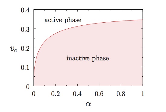
Figure 1: Nonequilibrium phase diagram of constrained adsorbtion dynamics: critical vacancy fraction $v_{\scriptscriptstyle\rm c}=1-\theta_{\scriptscriptstyle\rm c}$ vs. irreversibility parameter $\alpha$.

To assess the limit of our approximation we perform standard grand-canonical Monte Carlo simulations for a $1D$ substrate of size $N=2^{17}$ by using annealing rate sufficiently low as to avoid hysteresis effect in cooling-heating cycles (typically $10^{4}-10^{5}$ MC sweeps per unit of chemical potential). In Fig. 2 we compare the virtually exact MC simulations of $v_{\scriptscriptstyle\rm a}$ vs $v$, for some values of the irreversibility parameter $\alpha$, with the solution of Eq. (30). The agreement turns out to be excellent. A closer look at the data shows that discrepancies (necessarily expected) near the threshold can be appreciated in a log-scale plot when the irreversibility parameter $\alpha$ becomes vanishingly small, see Fig. 3, i.e., when the equilibrium limit of constrained adsorption-desorption dynamics is approached. Thus, the decoupling approximation becomes increasingly accurate in the limit of fully unconstrained desorption. Next-nearest neighbours correlation are, however, very important in determining the kinetic approach to the steady state, as the decoupling approximation does not close the dynamical hierarchy (22). The problem of addressing kinetics with a clever approximation scheme is therefore left to future work.

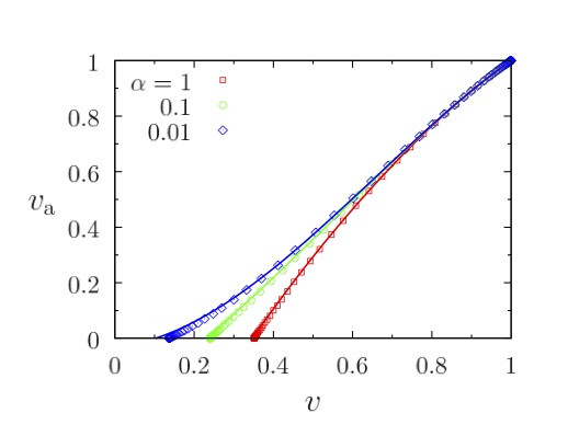
Figure 2: Fraction of available vacancies $v_{\scriptscriptstyle\rm a}$ vs. vacancy fraction $v$ for some values of the irreversibility parameter $\alpha$ (full lines are theoretical results, symbols are Monte Carlo data).

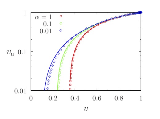
Figure 3: Same data as in Fig. 2 in a log-scale plot (highlighting the discrepancy between theoretical and numerical results at small $v_{\scriptscriptstyle\rm a}$).

To summarise we have introduced a simple model of adsorption-desorption dynamics with irreversible kinetic constraints and studied its steady state in one spatial dimension. We found a continuous nonequilibrium phase transition that is nicely captured by a naive mean-field approximation. In higher spatial dimensions a similar nonequilibrium transition should arguably occur, and it would be particularly interesting to investigate cooperative models in which adsorption is promoted by two or more nearby vacancies. We expect, in this case, a more subtle influence of the broken time-reversal symmetry on dynamics which, on a Bethe lattice, should lead to a nontrivial competition between hybrid and absorbing phase transitions. Including polydispersity in the present approach is also possible Prados_mixture , and could give rise to rather complex phase behaviours ArSe .

References

- (1) G.H. Fredrickson and H.C. Andersen, J. Chem. Phys. 83, 5822 (1985).
- (2) G.H. Fredrickson and S.A. Brawer, J. Chem. Phys. 84, 3351 (1986).
- (3) F. Ritort and P. Sollich, Adv. Phys. 52, 219 (2003).
- (4) J.P. Garrahan, P. Sollich and C. Toninelli, in: Dynamical Heterogeneities in Glasses, Colloids, and Granular Media (eds. L. Berthier, G. Biroli, J.-P. Bouchaud, L. Cipelletti and W. van Saarloos), pp. 341–369, Oxford University Press, 2011.
- (5) J. Marro and R. Dickman, Nonequilibrium phase transitions in lattice models, Cambridge University Press, 2005.
- (6) J.W. Evans, Rev. Mod. Phys. 65, 1281 (1993).
- (7) J.Talbot, G.Tarjus, P. R.Van Tassel, and P.Viot, Colloids Surfaces A165, 287 (2000).
- (8) X. Jin, G. Tarjus, and J. Talbot, J. Phys. A: Math. Gen. 27, L195 (1994).
- (9) P.L. Krapivsky and E. Ben‐Naim, J. Chem. Phys. 100, 6778 (1994).
- (10) E. Follana and F.Ritort, Phys. Rev. B 54, 930 (1996).
- (11) A. Crisanti, F. Ritort, A. Rocco, and M. Sellitto, J. Chem. Phys. 113, 10615 (2000).
- (12) A. Baule, F. Morone, H.J. Herrmann, and H.A. Makse, Rev. Mod. Phys. 90, 015006 (2018).
- (13) J. J. Brey, A. Prados, and B. Sánchez-Rey, Phys. Rev. E 60, 5685 (1999).
- (14) J.J. Brey, A. Prados, and B. Sánchez-Rey, Physica A 275, 310 (2000).
- (15) A. Prados and J.J Brey, Phys. Rev. E, 66, 041308 (2002).
- (16) A. Lefevre and D.S. Dean, J. Phys. A 34, L213 (2001).
- (17) J. Berg, S. Franz, and M. Sellitto, Eur. Phys. J. B 26, 349 (2002).
- (18) G. De Smedt, C. Godreche, and J.-M. Luck, Eur. Phys. J. B 27, 363 (2002).
- (19) A. Prados, and J.J Brey, J. Phys. A: Math. Gen. 38, 7051 (2005).
- (20) J. J. Arenzon and M. Sellitto, J. Chem. Phys. 137, 084501 (2012).