Minkowski symmetry sets for 1-parameter families of plane curves

Abstract

In this paper the generic bifurcations of the Minkowski symmetry set for 1-parameter families of plane curves are classified and the necessary and sufficient geometric criteria for each type are given. The Minkowski symmetry set is an analogue of the standard Euclidean symmetry set, and is defined to be the locus of centres of all its bitangent pseudo-circles. It is shown that the list of possible bifurcation types are different to those that occur in the list of possible types for the Euclidean symmetry set.

1 Introduction

Symmetry sets and related constructions have provided useful representations of shapes for object recognition as well as attracting interest in their own right and in the geometric properties of curves that they reveal. In the standard Euclidean plane, the (Euclidean) symmetry set of a curve $\gamma$ is defined as the locus of the centres of circles that are tangent to $\gamma$ in at least two distinct points (bitangent), see for example [3, 4]. The medial axis of $\gamma$ is a subset of its symmetry set, and is defined to be the locus of the centres of circles that are bitangent to $\gamma$ and completely contained in $\gamma$. Introduced by Blum in 1967 [1], the medial axis was originally designed as a tool for biological shape recognition and is also referred to as the central set, the topological skeleton, and the shock set for grassfire flows, see for example [5, 12].

The Minkowski symmetry set of a curve $\gamma$ was introduced in [13] as a Minkowski analogue of the (Euclidean) symmetry set. It is defined to be the locus of the centres of pseudo-circles that are bitangent to $\gamma$. In [10] the generic singularities of the Minkowski symmetry set were classified and the main result of the present paper is to extend this result to classify the generic singularities that occur for 1-parameter families of plane curves. A well-studied, closely related construct to the symmetry set called the medial axis, is the locus of bitangent circles completely contained within $\gamma$ and has found various applications in computer vision. A Minkowski version of the medial axis was introduced in [11].

In [3], the transitions that occur for (Euclidean) symmetry sets of 1-parameter families of curves are classified. Moreover, the complete list of full bifurcation sets for a generic family of functions are given, and it is demonstrated that certain transitions are excluded for geometrical reasons. Analogous to this, in the present paper the generic bifurcations of the Minkowski symmetry set for 1-parameter families of plane curves are classified and their criteria are determined.

Main Theorem 1.1

The possible transitions types of the Minkowski Symmetry set for a generic curve are $A_{1}^{4}(a),A_{1}^{4}(b),A_{2}^{2}(a),A_{2}^{2}(b)$, $A_{1}A_{3}(a)$, $A_{1}A_{3}(b)$, $A_{1}^{2}A_{2}(a)$, $A_{1}^{2}A_{2}(b)$ and $A_{4}$.

Remark 1.2

Note that the list of possible transitions types for the Minkowski Symmetry Set differs from that of the Euclidean Symmetry Set where only types $A_{1}^{4}(a),A_{2}^{2}(a),A_{2}^{2}(b),A_{1}A_{3}(a),A_{1}^{2}A_{2}(a)$ and $A_{4}$ can occur (see [3]).

Remark 1.3

For the Euclidean Medial Axis, only types $A_{1}^{4}(a),A_{1}A_{3}(a)$ can the centre be on the medial axis (see for example [7]). The Minkowski Medial Axis was defined in [11] as the locus of centres of pseudo-circles that are bitangent to $\gamma$ with one of its branches. It follows that only $A_{1}^{4}(b)$ and $A_{1}A_{3}(a)$ can have their centres on the Minkowski Medial Axis (see main text and Table on page 1).

Remark 1.4

In [8] the an Affine version of the Symmetry Set called the Affine Distance Symmetry Set was considered. It was shown that $A_{1}^{4}(a)$, $A_{1}^{4}(b)$,$A_{2}^{2}(a)$, $A_{2}^{2}(b)$, $A_{1}A_{3}(a)$, $A_{1}A_{3}(b)$, $A_{1}^{2}A_{2}(a)$, $A_{1}^{2}A_{2}(b)$ and $A_{4}$ could occur generically. In the case where $\gamma$ is an oval (a strictly convex, smooth and closed curve), it was also shown that $A_{1}^{4}(b),A_{1}^{2}A_{2}(b)$ and $A_{1}A_{3}(b)$ were prohibited.

	Euclidean	Minkowski	Affine
$A_{1}^{4}(a)$	$\checkmark$	Odd $\#$ points per branch	✓
$A_{1}^{4}(b)$	$\times$	Even $\#$ points per branch	Not for Ovals
$A_{2}^{2}(a)$	$\kappa_{1}^{\prime}\kappa_{2}^{\prime}>0$	$\kappa_{1}^{\prime}\kappa_{2}^{\prime}>0$ (M. Curvature)	✓
$A_{2}^{2}(b)$	$\kappa_{1}^{\prime}\kappa_{2}^{\prime}<0$	$\kappa_{1}^{\prime}\kappa_{2}^{\prime}<0$ (M. Curvature)	✓
$A_{1}A_{3}(a)$	✓	Points on different branches	✓
$A_{1}A_{3}(b)$	$\times$	Points on the same branch	Not for Ovals
$A_{1}^{2}A_{2}(a)$	✓	$A_{1}$ points on same branch	✓
$A_{1}^{2}A_{2}(b)$	$\times$	$A_{1}$ points on opposite branches	Not for Ovals
$A_{4}$	✓	✓	✓

2 The Minkowski pseudo-metric

The Minkowski plane $(\mathbb{R}_{1}^{2},\langle,\rangle)$ is the vector space $\mathbb{R}^{2}$ endowed with the pseudo-scalar product $\langle\mbox{\boldmath$u$},\mbox{\boldmath$v$}\rangle=-u_{0}v_{0}+u_{1}v_{1}$, for any $\mbox{\boldmath$u$}=(u_{0},u_{1})$ and $\mbox{\boldmath$v$}=(v_{0},v_{1})$. A vector $\mbox{\boldmath$u$}\in\mathbb{R}^{2}_{1}$ is called timelike if $\langle\mbox{\boldmath$u$},\mbox{\boldmath$u$}\rangle<0$, spacelike if $\langle\mbox{\boldmath$u$},\mbox{\boldmath$u$}\rangle>0$, and lightlike if $\langle\mbox{\boldmath$u$},\mbox{\boldmath$u$}\rangle=0$.

The norm of $u$ is defined by $||\mbox{\boldmath$u$}||=\sqrt{|\langle\mbox{\boldmath$u$},\mbox{\boldmath$u$}\rangle|}$, and the perpendicular operator $\perp$ assigns ${\bf u}^{\perp}=(u_{1},u_{0})$.

There are three distinct types of pseudo-circles in $\mathbb{R}^{2}_{1}$ with centre $c\in\mathbb{R}^{2}_{1}$ and radius $r$, $r>0$, are defined as follows:

$$H^{1}(c,-r) = \{p\in\mathbb{R}^{2}_{1}\,|\,\langle p-c,p-c\rangle=-r^{2}\},$$

$$S^{1}_{1}(c,r) = \{p\in\mathbb{R}^{2}_{1}\,|\,\langle p-c,p-c\rangle=r^{2}\},$$

$$LC^{*}(c) = \{p\in\mathbb{R}^{2}_{1}\setminus\{{\bf 0}\}\,|\,\langle p-c,p-c\rangle=0\}.$$

Observe that $LC^{*}(c)$ is the union of the two lines through $c$ with tangent directions $(1,1)$ and $(1,-1)$, with the point $c$ removed. The pseudo-circle $H^{1}(c,-r)$ has two branches which can be parametrised by $c+(\pm r\cosh(t),r\sinh(t))$, $t\in\mathbb{R}$. The pseudo-circle $S^{1}(c,r)$ is also composed of two branches and these can be parametrised by $c+(r\sinh(t),\pm r\cosh(t))$, $t\in\mathbb{R}$.

Let $\gamma:S^{1}\to\mathbb{R}^{2}_{1}$ be an immersion, where $S^{1}$ is the unit Euclidean circle. Call the curve $\gamma$ the image of the map $\gamma$ and say that it is a closed smooth curve (that is, $\gamma$ is a regular closed curve and may have points of self-intersection).

The curve $\gamma$ at $t_{0}$ is said to be spacelike if $\gamma^{\prime}(t_{0})$ is spacelike and is said to be timelike if $\gamma^{\prime}(t_{0})$ timelike. These are open properties so there is a neighbourhood of $t_{0}$ where the curve is either spacelike or timelike. If $\gamma^{\prime}(t_{0})$ is lightlike then $\gamma(t_{0})$ is said to be a lightlike point. It is shown in [13] that the set of lightlike points of $\gamma$ is the union of at least four disjoint non-empty and closed subsets of $\gamma$. The complement of these sets are disjoint connected spacelike or timelike pieces of the curve $\gamma$.

The spacelike and timelike components of $\gamma$ can be parametrised by arc length. Suppose that $\gamma(s)$, $s\in(\lambda,\mu)$, is an arc length parametrisation of a component of $\gamma$. Then $\mbox{\boldmath$t$}(s)=\gamma^{\prime}(s)$ is a unit tangent vector and $\mbox{\boldmath$t$}^{\prime}(s)=\kappa(s)\mbox{\boldmath$n$}(s)$, where $\kappa(s)$ is the Minkowski curvature of $\gamma$ at $s$ and $n$ is the unit normal vector at $s$. The tangent and unit normal vectors are pseudo-orthogonal so they are of different types, that is, one is spacelike and the other is timelike.

When $\gamma$ is not necessarily parametrised by arclength, the unit tangent is given by

$$T(t)=\frac{\gamma^{\prime}(t)}{|\langle\gamma^{\prime}(t),\gamma^{\prime}(t)\rangle|^{\frac{1}{2}}},$$

the unit normal by

$$N(t)=(-1)^{\beta}T(t),$$

where $\beta=1$ if $\gamma$ is spacelike and $\beta=2$ if $\gamma$ is timelike, and the Minkowski curvature (dropping the parameter $t$) is given by

$$\kappa=\frac{\langle\gamma^{\prime},\gamma^{\prime\prime\perp}\rangle}{|\langle\gamma^{\prime},\gamma^{\prime}\rangle|^{\frac{3}{2}}}.$$

3 The Minkowski Symmetry Set

The evolute of a spacelike or timelike component of $\gamma$ is the image of the map

$$e(t)=\gamma(t)-\frac{1}{\kappa(t)}N(t).$$

In general, the curvature tends to infinity as $t$ tends to $\lambda$ or $\mu$ and the evolute of the curve $\gamma$ is not defined at the lightlike points. However, the caustic of $\gamma$ is defined everywhere and contains the evolute of $\gamma$ (see for example [13]). The caustic can be defined via the the family of distance-squared functions $f:S^{1}\times\mathbb{R}^{2}_{1}\to\mathbb{R}$ on $\gamma$ given by

$$f(t,c)=\langle\gamma(t)-c,\gamma(t)-c\rangle.$$

Denote by $f_{c}:S^{1}\to\mathbb{R}$ the function given by $f_{c}(t)=f(t,c)$. We say that $f_{c}$ has an $A_{k}$-singularity at $t_{0}$ if $f_{c}^{\prime}(t_{0})=f_{c}^{\prime\prime}(t_{0})=\ldots=f_{c}^{(k)}(t_{0})=0$ and $f_{c}^{(k+1)}(t_{0})\neq 0$. This is equivalent to the existence of a local re-parametrisation $h$ of $\gamma$ at $t_{0}$ such that $(f\circ h)(t)=\pm t^{k+1}$. Geometrically, $f_{c}$ has an $A_{k}$-singularity if and only if the curve $\gamma$ has contact of order $k+1$ at $\gamma(t_{0})$ with the pseudo-circle of centre $c$ and radius $r$, with $r=\langle\gamma(t_{0})-c,\gamma(t_{0})-c\rangle$. Thus, the curve $\gamma$ has order of contact 1 with a pseudo-circle at $t_{0}$ if it intersects transversally the pseudo-circle at $\gamma(t_{0})$. The order of contact is 2 if the circle and the curve have ordinary tangency at $\gamma(t_{0})$.

The caustic of $\gamma$ is the local component $\mathcal{B}_{1}$ of the bifurcation set of the family $f$, given by

$$\mathcal{B}_{1}=\{c\in\mathbb{R}^{2}_{1}\,|\,\exists t\in S^{1}\mbox{ such that }f_{c}^{\prime}(t)=f_{c}^{\prime\prime}(t)=0\}.$$

This is the set of points $c\in\mathbb{R}^{2}_{1}$ such that the germ $f_{c}$ has a degenerate singularity at some point $t$. In [13] it was shown that the caustic of $\gamma$ is defined at all points on $\gamma$ including its lightlike points where it is a smooth curve and has ordinary tangency with $\gamma$.

The multi-local component of the bifurcation set of the family $f$ is defined as

$$\mathcal{B}_{2}=\{c\in\mathbb{R}^{2}_{1}\,|\,\exists t_{1},t_{2}\mbox{ such that }t_{1}\neq t_{2},\ f_{c}(t_{1})=f_{c}(t_{2}),\,f_{c}^{\prime}(t_{1})=f_{c}^{\prime}(t_{2})=0\}.$$

The full-bifurcation set of $f$ is defined as

$$\mbox{\rm Bif}(f)=\mathcal{B}_{1}\cup\mathcal{B}_{2}.$$

Definition 3.1

The Minkowski Symmetry Set (MSS) of $\gamma$ is the locus of centres of pseudo-circles which are tangent to $\gamma$ in at least two distinct points $p$ and $q$. The pairs of points $p,q$ are called bi-tangent pairs.

The $MSS$ is precisely the multi-local component $\mathcal{B}_{2}$ of the bifurcation set of the family of distance-squared function $f$ on $\gamma$.

In [10] it is shown that the singularities which can occur on the MSS for a generic plane curve are $A_{1}$, $A_{2},A_{1}^{3},A_{2}A_{1}$ and $A_{3}$, and that they are all versally unfolded. It follows that these singularities are also versally unfolded for a 1-parameter of plane curves. It can happen for a generic 1-parameter family of plane curves that at isolated points one of the above singularities occurs at lightlike points and this case is also dealt with in [10]. It only remains now to show the versality and the transition type for the other generically occurring singularities for a 1-parameter family of plane curves, namely $A_{1}^{4},A_{2}A_{1}^{2},A_{3}A_{1},A_{2}^{2}$ and $A_{4}$.

In [3] it was shown that for general functions some of these singularities occur in two distinct transition types. For example, in the $A_{1}^{4}$ case there exist two types referred to as $A_{1}^{4}(a)$ and $A_{1}^{4}(b)$. It was shown in that paper that only types $A_{1}^{4}(a),A_{2}^{2}(a),A_{2}^{2}(b),A_{1}A_{3}(a),A_{1}^{2}A_{2}(a)$ and $A_{4}$ could occur for (Euclidean) symmetry sets (see Table on 1). In the present paper a similar analysis is carried out for the Minkowski symmetry set and the geometric conditions for the possible types are determined. In particular, the following theorem is proven:

Theorem 3.2

The possible transitions types of the Minkowski Symmetry set for a generic curve are $A_{1}^{4}(a),A_{1}^{4}(b),A_{2}^{2}(a),A_{2}^{2}(b)$, $A_{1}A_{3}(a)$, $A_{1}A_{3}(b)$, $A_{1}^{2}A_{2}(a)$, $A_{1}^{2}A_{2}(b)$ and $A_{4}$.

Each generically occurring singularity type is considered in turn. Considering the reduction of the distance-squared family to its normal form, the necessary geometrical criteria for each transition type (eg. $a$ or $b$) is determined.

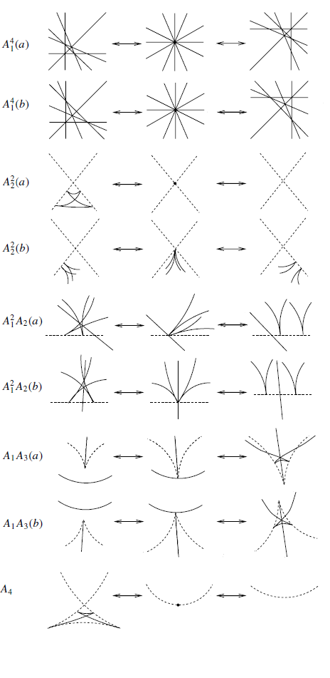
Figure 1: The Transitions that can occur on Minkowski Symmetry Sets.

4 The $A_{1}^{4}$ singularity

Consider the standard multi-versal unfolding of an $A_{1}^{4}$ singularity given by

$$G:\mathbb{R}^{(4)}\times\mathbb{R}^{3}\to\mathbb{R},$$

where $\mathbb{R}^{(4)}$ denotes the set of parameters $t_{1},t_{2},t_{3},t_{4}$, $\mathbb{R}^{3}$ denotes the $(y_{1},y_{2},y_{3})$-space of unfolding parameters and the multi-versal unfolding $G$ is given by

$$G_{i} : (t_{i},\mbox{\boldmath$y$})\mapsto t_{i}^{2}+y_{i},i=1,2\ {\rm and}\ 3$$

$$G_{4} : (t_{4},\mbox{\boldmath$y$})\mapsto t_{4}^{2}.$$

Consider now four families of curve segments $\gamma_{1},\mbox{$\gamma$}_{2},\mbox{$\gamma$}_{3}$ and $\mbox{$\gamma$}_{4}$ each being close to one of the tangency points. With family parameter $u$, denote these segments as $\mbox{$\gamma$}_{i,u}(s_{i})=(X_{i,u}(s_{i}),Y_{i,u}(s_{i}))$, where the arclength parameters $s_{i}$ are close to zero. Take ${\mbox{\boldmath$x$}}=(x_{1},x_{2})\in\mathbb{R}^{2}_{1}$, and denote by $\mbox{\boldmath$x$}_{0}$ the $A_{1}^{4}$-point on the MSS. Then the family of Minkowski distance functions on the family of curve segments consists of four germs

$$F_{i}:\mathbb{R}\times\mathbb{R}\times\mathbb{R}^{2}_{1},(0,0,\mbox{\boldmath$x$}_{0})\to\mathbb{R},$$

given by

$$F_{i}(s_{i},u,\mbox{\boldmath$x$})=\langle\mbox{\boldmath$x$}-\mbox{$\gamma$}_{i,u},\mbox{\boldmath$x$}-\mbox{$\gamma$}_{i,u}\rangle.$$

Using standard techniques, as outlined in [3], and used for example in [8] and [9], is to reduce the family $F_{i}$ to the standard family $G_{i}$. The big bifurcation set (BBS), which sits in $y$-space and comprises of subsets which correspond to $A_{1}^{2}$ sets of $G$, contains all the possible types bifurcations of $A_{1}^{4}$, and the individual bifurcation sets can be recovered locally by slicing the BBS with non-singular families of surfaces passing through the origin in $y$-space. Firstly, the possible generic transition types and their criteria are found, and then through keeping track of the geometric properties in reducing the family to the standard type, the relevant bifurcation type can be determined.

4.1 Bad planes

Following [3], a plane containing the origin given by the equation $a_{1}y_{1}+a_{2}y_{2}+a_{3}y_{3}=0$ is called a bad plane if it contains any of the limiting tangent vectors to the strata of the big bifurcation set of $G$. Non-generic transitions occur when these slicing surfaces are themselves tangent to the limiting tangent vectors to the strata of the big bifurcation set tending to the origin. A plane can be represented by a point with homogenous coordinates $(a_{1}:a_{2}:a_{3})$ in the real projective plane $\mathbb{R}P^{2}$ and the pencils of bad planes therefore correspond to lines in $\mathbb{R}P^{2}$.

If $\Delta$ represents the se of bad planes each component of $\mathbb{R}P^{2}-\Delta$ represent collections of normals, which as kernels of $dh(0)$ give $C^{0}$-stratified equivalent functions of $h$. (For remarks on stratified equivalence see for example [3] and [2].) Each connects component of $\mathbb{R}P^{2}-\Delta$ can potentially give a different type of transition. By considering each region in turn and identifying the type of transition it is possible to determine the criteria for realising each one.

The one-dimensional strata adjacent to the BBS for the standard $A_{1}^{4}$ are

$$A_{1}^{3} : \{(a_{1},a_{2},a_{3})=(t_{1},t_{1},t_{1})\cup(t_{1},0,0)\cup(0,0,t_{2})\cup(0,0,t_{3})\}$$

$$A_{1}^{2}/A_{1}^{2} : \{(a_{1},a_{2},a_{3})=(t_{1},t_{1},0)\cup(0,t_{2},t_{2})\cup(t_{3},0,t_{3})\}.$$

The limiting tangent vectors to these one-dimensional strata are therefore given by $(1,0,0),(0,1,0),(0,0,1)$, $(1,1,1)$, $(1,1,0),(0,1,1)$, and $(1,0,1)$ so the bad planes are given by $a_{1}=0$, $a_{2}=0$, $a_{3}=0$, and $a_{1}+a_{2}+a_{3}=0$, $a_{1}+a_{2}=0$, $a_{2}+a_{3}=0$, and $a_{1}+a_{3}=0$.

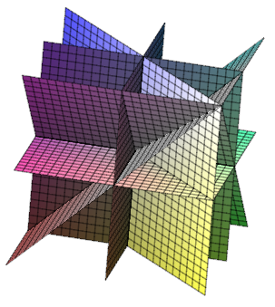
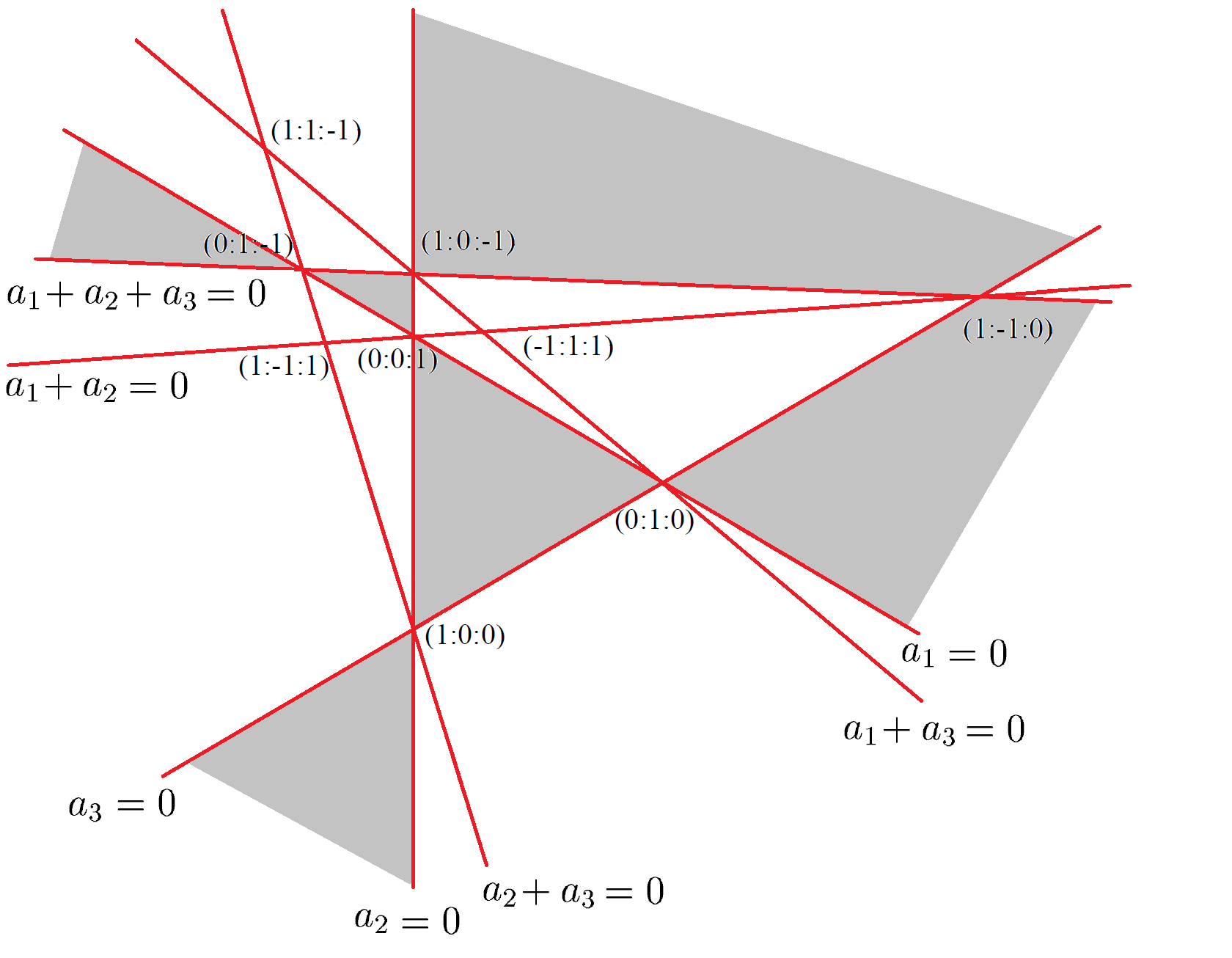
Figure 3: Left: The BBS for $A_{1}^{4}$. Right: The regions determining the different types for $A_{1}^{4}$.

It is determined that the shaded regions of Figure 3 (right) correspond to one type of transition and the non-shaded regions give another from which the following proposition can be deduced.

Proposition 4.1

If $a_{1}a_{2}a_{3}(a_{1}+a_{2}+a_{3})$ is negative the point $(a_{1}:a_{2}:a_{3})$ lies in the shaded region of Figure 3 (right) and the corresponding full bifurcation set has type $A_{1}A_{3}(a)$. If however $a_{1}a_{2}a_{3}(a_{1}+a_{2}+a_{3})$ is positive, then the point lies in the unshaded region and the corresponding full bifurcation set is of type $A_{1}A_{3}(b)$.

Since it is assumed that each $F_{i}$ is a multi-versal unfolding, then by the uniqueness of multi-versal unfoldings each of the unfoldings $G_{i}$ in the standard multi-versal unfolding $G$ can be induced from the affine distance functions $F_{i}$ by

$$G_{i}(t_{i},\mbox{\boldmath$y$})=F_{i}(A_{i}(t_{i},\mbox{\boldmath$y$}),B(\mbox{\boldmath$y$}))+C(\mbox{\boldmath$y$}),{\rm for\ }i=1,2,3{\rm\ and\ }4,$$ (1)

where each $A_{i}:\mathbb{R}\times\mbox{$\mathbb{R}$}^{3}\to\mbox{$\mathbb{R}$}$ is a germ at $(0,{\bf 0})$ and $B,C$ denote the germs $B:(\mbox{$\mathbb{R}$}^{3},{\bf 0})\to(\mbox{$\mathbb{R}$}\times\mbox{$\mathbb{R}$}^{2},(0,\mbox{\boldmath$x$}_{0}))$ and $C:(\mbox{$\mathbb{R}$}^{3},{\bf 0})\to(\mbox{$\mathbb{R}$},d_{0}).$

$$\begin{CD}\mbox{$\mathbb{R}$}\times\mbox{$\mathbb{R}$}^{3}@>{G}>{}>\mbox{$\mathbb{R}$}\times\mbox{$\mathbb{R}$}^{3}@>{}>{}>\mbox{$\mathbb{R}$}^{3}@>{h}>{}>\mbox{$\mathbb{R}$}\\ @V{}V{(A_{i}\times B)}V@V{}V{(-C\times B)}V@V{}V{B}V@V{}V{\rm identity}V\\ C@>{F}>{}>D@>{}>{}>D@>{\pi_{1}}>{}>\mbox{$\mathbb{R}$}\end{CD}$$

From the commutative diagram it can be seen that $h=\pi_{1}\circ B$, where $\pi_{1}$ denotes projection onto the first coordinate. Thus, $B_{1}$ (where $B_{i}$ denotes the $i^{th}$ component of $B$) is the map $h$ on the standard $A_{1}^{4}$ set (the BBS), which corresponds to the plane through the origin in $y$-space representing the tangent plane to the surface with which we are slicing the BBS. This tangent plane thus corresponds to the kernel of the map $h$ on the BBS, i.e.

$${\rm ker}\ dB_{1}:\mbox{$\mathbb{R}$}^{3}\to\mbox{$\mathbb{R}$},\ {\rm with\ matrix\ }\left.\left(\frac{\partial B_{1}}{\partial y_{1}},\frac{\partial B_{2}}{\partial y_{2}},\frac{\partial B_{3}}{\partial y_{3}}\right)\right|_{\mbox{\boldmath$y$}={\bf 0}}.$$

Hence the kernel plane has equation

$$\left.\left.\left.\frac{\partial B_{1}}{\partial y_{1}}\right|_{\mbox{\boldmath$y$}={\bf 0}}y_{1}+\frac{\partial B_{2}}{\partial y_{2}}\right|_{\mbox{\boldmath$y$}={\bf 0}}y_{2}+\frac{\partial B_{3}}{\partial y_{3}}y_{3}\right|_{\mbox{\boldmath$y$}={\bf 0}}=0.$$

Proposition 4.2

The MSS has a transition of type $A_{1}^{4}(a)$ if there are odd number of points on each branch and is of type $A_{1}^{4}(b)$ if there are an even number of points on each branch.

Proof. Consider the case $i=1$:

$$\left.\left(\frac{\partial G_{1}}{\partial t_{1}}\ \frac{\partial G_{1}}{\partial y_{1}}\ \frac{\partial G_{1}}{\partial y_{2}}\ \frac{\partial G_{1}}{\partial y_{3}}\right)\right|_{\mbox{\boldmath$y$}={\bf 0}}=(2t_{1}\ 1\ 0\ 0).$$

Using relation (1) and applying the chain rule for derivatives gives:

$$=\left.\left(\frac{\partial F_{1}}{\partial s_{1}}\ \frac{\partial F_{1}}{\partial x_{1}}\ \frac{\partial F_{1}}{\partial x_{2}}\ \frac{\partial F_{1}}{\partial x_{3}}\right)\right|_{(A_{1}(t_{1},{\bf 0}),\mbox{\boldmath$x$}_{0})}\times\left.\left(\begin{array}[]{cccc}\frac{\partial A_{1}}{\partial t_{1}}&\frac{\partial A_{1}}{\partial y_{1}}&\frac{\partial A_{1}}{\partial y_{2}}&\frac{\partial A_{1}}{\partial y_{3}}\\ 0&\frac{\partial B_{1}}{\partial y_{1}}&\frac{\partial B_{1}}{\partial y_{2}}&\frac{\partial B_{1}}{\partial y_{3}}\\ 0&\frac{\partial B_{2}}{\partial y_{1}}&\frac{\partial B_{2}}{\partial y_{2}}&\frac{\partial B_{2}}{\partial y_{3}}\\ 0&\frac{\partial B_{3}}{\partial y_{1}}&\frac{\partial B_{3}}{\partial y_{2}}&\frac{\partial B_{3}}{\partial y_{3}}\end{array}\right)\right|_{(t_{1},{\bf 0})}+\left.\left(0\ \frac{\partial C}{\partial y_{1}}\ \frac{\partial C}{\partial y_{2}}\ \frac{\partial C}{\partial y_{3}}\right)\right|_{\mbox{\boldmath$y$}={\bf 0}}$$

The same can be done for $G_{2},G_{3}$ and $G_{4}$, which have the right side of the first line as $(2t_{2}\ 0\ 1\ 0)$, $(2t_{3}\ 0\ 0\ 1)$ and $(2t_{4}\ 0\ 0\ 0)$ respectively. Now $\frac{\partial F_{i}}{\partial s_{i}}(0,\mbox{\boldmath$x$}_{0})\equiv 0$ because $F_{i}$ has an $A_{1}$ singularity at $(0,\mbox{\boldmath$x$}_{0})$. Also, $\frac{\partial F_{i}}{\partial x_{1}}=-2x_{1}+2X_{u,i}(s_{i}),\frac{\partial F_{i}}{\partial x_{2}}=2x_{2}-2Y_{u,i}(s_{i}).$ The substitution $t_{i}=0$ can be made since only the 0-jets are required.

Taking all the $G_{i}$ together gives the system:

$$\left(\begin{array}[]{ccc}1&0&0\\ 0&1&0\\ 0&0&1\\ 0&0&0\end{array}\right)=\left.\left(\begin{array}[]{ccc}\frac{\partial F_{1}}{\partial u}&\frac{\partial F_{1}}{\partial x_{1}}&\frac{\partial F_{1}}{\partial x_{2}}\\ \frac{\partial F_{2}}{\partial u}&\frac{\partial F_{2}}{\partial x_{1}}&\frac{\partial F_{2}}{\partial x_{2}}\\ \frac{\partial F_{3}}{\partial u}&\frac{\partial F_{3}}{\partial x_{1}}&\frac{\partial F_{3}}{\partial x_{2}}\\ \frac{\partial F_{4}}{\partial u}&\frac{\partial F_{4}}{\partial x_{1}}&\frac{\partial F_{4}}{\partial x_{2}}\end{array}\right)\right|_{(A(t_{i},{\bf 0}),\mbox{\boldmath$x$}_{0})}\times JB+\left(\begin{array}[]{c}JC\\ JC\\ JC\\ JC\end{array}\right)$$ (14)

where, for conciseness, $JB$ and $JC$ denote the matrices

$$JB=\left.\left(\begin{array}[]{ccc}\frac{\partial B_{1}}{\partial y_{1}}&\frac{\partial B_{1}}{\partial y_{2}}&\frac{\partial B_{1}}{\partial y_{3}}\\ \frac{\partial B_{2}}{\partial y_{1}}&\frac{\partial B_{2}}{\partial y_{2}}&\frac{\partial B_{2}}{\partial y_{3}}\\ \frac{\partial B_{3}}{\partial y_{1}}&\frac{\partial B_{3}}{\partial y_{2}}&\frac{\partial B_{3}}{\partial y_{3}}\end{array}\right)\right|_{\mbox{\boldmath$y$}=0},\ \ \ JC=\left.\left(\begin{array}[]{ccc}\frac{\partial C}{\partial y_{1}}&\frac{\partial C}{\partial y_{2}}&\frac{\partial C}{\partial y_{3}}\end{array}\right)\right|_{\mbox{\boldmath$y$}=0}.$$

Subtracting the bottom row from the other rows in equation (14) gives

$$\left(\begin{array}[]{ccc}1&0&0\\ 0&1&0\\ 0&0&1\\ 0&0&0\end{array}\right)=\left.\left(\begin{array}[]{ccc}\frac{\partial F_{1}}{\partial u}-\frac{\partial F_{4}}{\partial u}&\frac{\partial F_{1}}{\partial x_{1}}-\frac{\partial F_{4}}{\partial x_{1}}&\frac{\partial F_{1}}{\partial x_{2}}-\frac{\partial F_{4}}{\partial x_{2}}\\ \frac{\partial F_{2}}{\partial u}-\frac{\partial F_{4}}{\partial u}&\frac{\partial F_{2}}{\partial x_{1}}-\frac{\partial F_{4}}{\partial x_{1}}&\frac{\partial F_{2}}{\partial x_{2}}-\frac{\partial F_{4}}{\partial x_{2}}\\ \frac{\partial F_{3}}{\partial u}-\frac{\partial F_{4}}{\partial u}&\frac{\partial F_{3}}{\partial x_{1}}-\frac{\partial F_{4}}{\partial x_{1}}&\frac{\partial F_{3}}{\partial x_{2}}-\frac{\partial F_{4}}{\partial x_{2}}\\ \frac{\partial F_{4}}{\partial u}&\frac{\partial F_{4}}{\partial x_{1}}&\frac{\partial F_{4}}{\partial x_{2}}\end{array}\right)\right|_{(A(t_{i},{\bf 0}),\mbox{\boldmath$x$}_{0})}\times JB+\left(\begin{array}[]{c}{\bf 0}\\ {\bf 0}\\ {\bf 0}\\ $JC$\end{array}\right).$$

Substituting $\frac{\partial F_{i}}{\partial x_{1}}$ and $\frac{\partial F_{i}}{\partial x_{2}}$ and ignoring the last row yields the following system:

$$I_{3}=\left(\begin{array}[]{ccc}\frac{\partial F_{1}}{\partial u}-\frac{\partial F_{4}}{\partial u}&X_{1}-X_{4}&-Y_{1}+Y_{4}\\ \frac{\partial F_{2}}{\partial u}-\frac{\partial F_{4}}{\partial u}&X_{2}-X_{4}&-Y_{2}+Y_{4}\\ \frac{\partial F_{3}}{\partial u}-\frac{\partial F_{4}}{\partial u}&X_{3}-X_{4}&-Y_{3}+Y_{4}\\ \end{array}\right)\times\left(\begin{array}[]{ccc}\frac{\partial B_{1}}{\partial y_{1}}&\frac{\partial B_{1}}{\partial y_{2}}&\frac{\partial B_{1}}{\partial y_{3}}\\ \frac{\partial B_{2}}{\partial y_{1}}&\frac{\partial B_{2}}{\partial y_{2}}&\frac{\partial B_{2}}{\partial y_{3}}\\ \frac{\partial B_{3}}{\partial y_{1}}&\frac{\partial B_{3}}{\partial y_{2}}&\frac{\partial B_{3}}{\partial y_{3}}\end{array}\right)$$

where $I_{3}$ represents the $(3\times 3)$ identity matrix.

The derivatives of $B_{1}$ can now be evaluated. Since the product of the two matrices is the identity, they must be inverse to each other. Now, the inverse of the first matrix can be used to calculate the required entries of the second matrix. So,

$$\frac{\partial B_{1}}{\partial y_{1}}=\beta{\rm det}\left(\begin{array}[]{cc}X_{2}-X_{4}&-Y_{2}+Y_{4}\\ X_{3}-X_{4}&-Y_{3}+Y_{4}\end{array}\right).$$

Multiplying the second column by $-1$ gives

$$\frac{\partial B_{1}}{\partial y_{1}}=-\beta{\rm det}\left(\begin{array}[]{cc}X_{2}-X_{4}&Y_{2}-Y_{4}\\ X_{3}-X_{4}&Y_{3}-Y_{4}\end{array}\right).$$

Similarly,

$$\frac{\partial B_{1}}{\partial y_{2}}=-\beta{\rm det}\left(\begin{array}[]{cc}X_{1}-X_{4}&Y_{1}-Y_{4}\\ X_{3}-X_{4}&Y_{3}-Y_{4}\end{array}\right),$$

$$\frac{\partial B_{1}}{\partial y_{3}}=-\beta{\rm det}\left(\begin{array}[]{cc}X_{1}-X_{4}&Y_{1}-Y_{4}\\ X_{2}-X_{4}&Y_{2}-Y_{4}\end{array}\right).$$

Let $q_{1}=\mbox{$\gamma$}_{2}-\mbox{$\gamma$}_{3}$, $q_{2}=\mbox{$\gamma$}_{3}-\mbox{$\gamma$}_{4}$, $q_{3}=\mbox{$\gamma$}_{4}-\mbox{$\gamma$}_{1}$ and $q_{4}=\mbox{$\gamma$}_{1}-\mbox{$\gamma$}_{2}$. Now, $\frac{\partial B_{1}}{\partial y_{1}}=-\beta{\rm det}\left(\genfrac{}{}{0.0pt}{}{q_{1}}{q_{2}}\right)$, $\frac{\partial B_{1}}{\partial y_{2}}=\beta{\rm det}\left(\genfrac{}{}{0.0pt}{}{q_{2}}{q_{3}}\right)$, $\frac{\partial B_{1}}{\partial y_{3}}=-\beta{\rm det}\left(\genfrac{}{}{0.0pt}{}{q_{3}}{q_{4}}\right)$, and $\frac{\partial B_{1}}{\partial y_{1}}+\frac{\partial B_{1}}{\partial y_{2}}+\frac{\partial B_{1}}{\partial y_{3}}=-\beta{\rm det}\left(\genfrac{}{}{0.0pt}{}{q_{3}}{q_{4}}\right)$.

Now ${\rm det}(q_{i},q_{j})>0$ if and only if the anticlockwise (Euclidean) angle from $q_{i}$ to $q_{j}$ is less than $\pi$. It then follows that $\frac{\partial B_{1}}{\partial y_{1}}\frac{\partial B_{1}}{\partial y_{2}}\frac{\partial B_{1}}{\partial y_{3}}\left(\frac{\partial B_{1}}{\partial y_{1}}+\frac{\partial B_{1}}{\partial y_{2}}+\frac{\partial B_{1}}{\partial y_{3}}\right)>0$ if and only if no point $p_{i}$ is inside the triangle formed by the other three $p_{j}$. This condition fails if and only if there are an even number of points on each branch and the resulting singularity is of type $A_{1}^{4}(b)$. On the other hand, if one of the branches contains only one point, and the other branch contains three, then the triangle formed by the point on the first branch and the ‘outer’ two points of the branch of three will necessarily contain the fourth point (see figure 2) and the singularity will be of type $A_{1}^{4}(a)$.

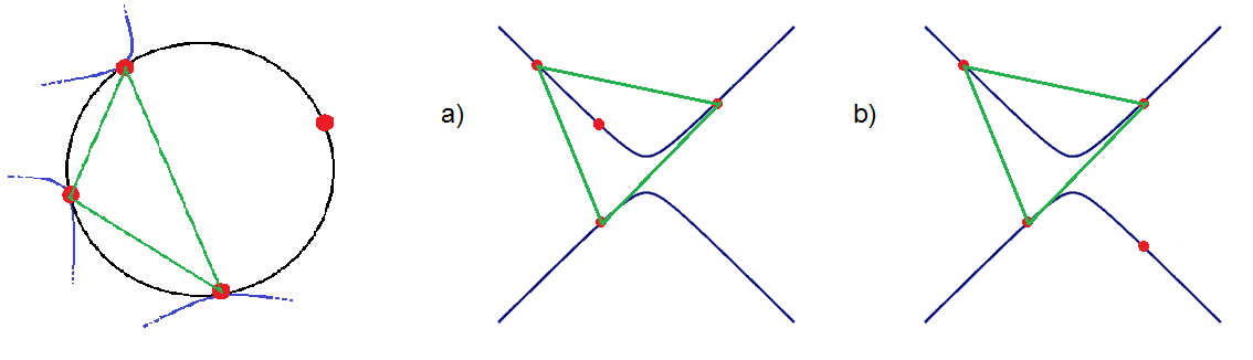
Figure 2: Left: Given three points on a circle, a fourth point necessarily lies outsied the triangle formed by the other three. Right: Given three points on a pseudo-circle, a fourth point can either lie inside (resulting in singularity $A_{1}^{4}(a)$), or outside the triangle formed by the other three (resulting in the singularity $A_{1}^{4}(b))$.

5 The $A_{2}^{2}$ singularity

Consider the following standard multi-versal unfolding of an $A_{1}^{2}A_{2}$ singularity given by

$$G:\mathbb{R}^{(2)}\times\mathbb{R}^{3}\to\mbox{$\mathbb{R}$}$$

where $\mathbb{R}^{(2)}$ denotes the parameters $t_{1},t_{2}$ and $\mathbb{R}^{3}$ denotes the unfolding parameters $\mbox{\boldmath$a$}=(a_{1},a_{2},a_{3})$ and the multi-versal unfolding is given by the two unfoldings:

$$G_{1}(t_{1},\mbox{\boldmath$a$}) = t_{1}^{3}+a_{1}t_{1}+a_{2},$$

$$G_{2}(t_{2},\mbox{\boldmath$a$}) = t_{2}^{3}+a_{3}t_{2}.$$

5.1 The bad planes

The one-dimensional strata adjacent to $A_{2}^{2}$ are

$$A_{1}A_{2} : \{(a_{1},a_{2},a_{3})=(-3t_{1}^{2},2t_{1}^{3},0)\cup(0,-2t_{2}^{3},-3t_{2}^{2})\}$$

$$A_{1}^{2}/A_{1}^{2} : \{(a_{1},a_{2},a_{3})=(-3t_{2}^{2},0,-3t_{2}^{2})\}.$$

The limiting tangent vectors to these one-dimensional strata are given by $(1,0,0),(0,1,0)$ and $(1,1,0)$ so the bad planes are given b $a_{1}=0$, $a_{3}=0$ and $a_{1}+a_{3}=0$.

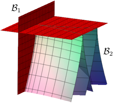
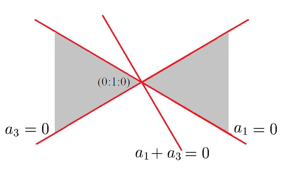
Figure 4: Left: The BBS for $A_{2}^{2}$. Right: The regions determining the different types for $A_{2}^{2}$.

Similarly to the previous case, the following proposition can be deduced.

Proposition 5.1

If $a_{1}a_{2}$ is negative the point $(a_{1}:a_{2}:a_{3})$ lies in the unshaded region of Figure 4 (right) and the corresponding full bifurcation set has type $A_{2}^{2}(a)$. If however $a_{1}a_{3}$ is positive, then the point lies in the shaded region and the corresponding full bifurcation set is of type $A_{2}^{2}(b)$.

The Minkowski distance function on the two curve segments near the $A_{2}^{2}$ points consists of the two germs

$$F_{1}(t_{1},u,x)=\langle\gamma_{1}(t_{1},u)-x,\gamma_{1}(t_{1},u)-x\rangle$$

$$F_{2}(t_{2},u,x)=\langle\gamma_{2}(t_{2},u)-x,\gamma_{2}(t_{2},u)-x\rangle.$$

To reduce to $G_{1}$ and $G_{2}$, as in the $A_{1}^{4}$ case, using (1) and applying the chain rule gives the system:

$$\left(\begin{array}[]{ccc}1&0&0\\ 0&1&0\\ 0&0&1\\ 0&0&0\end{array}\right)=\left.\left(\begin{array}[]{ccc}\frac{\partial^{2}F_{1}}{\partial t_{1}\partial u}&\frac{\partial^{2}F_{1}}{\partial t_{1}\partial x_{1}}&\frac{\partial^{2}F_{1}}{\partial t_{1}\partial x_{2}}\\ \frac{\partial F_{1}}{\partial u}&\frac{\partial F_{1}}{\partial x_{1}}&\frac{\partial F_{1}}{\partial x_{2}}\\ \frac{\partial^{2}F_{2}}{\partial t_{2}\partial u}&\frac{\partial^{2}F_{2}}{\partial t_{2}\partial x_{1}}&\frac{\partial^{2}F_{2}}{\partial t_{2}\partial x_{2}}\\ \frac{\partial F_{2}}{\partial u}&\frac{\partial F_{2}}{\partial x_{1}}&\frac{\partial F_{2}}{\partial x_{2}}\end{array}\right)\right|_{(A(t_{i},{\bf 0}),\mbox{\boldmath$x$}_{0})}\times JB+\left(\begin{array}[]{c}{\bf 0}\\ JC\\ {\bf 0}\\ JC\end{array}\right).$$

Subtracting the bottom row from the second and then ignoring the bottom yields

$$\left(\begin{array}[]{ccc}1&0&0\\ 0&1&0\\ 0&0&1\end{array}\right)=\left.\left(\begin{array}[]{ccc}\frac{\partial^{2}F_{1}}{\partial t_{1}\partial u}&\frac{\partial^{2}F_{1}}{\partial t_{1}\partial x_{1}}&\frac{\partial^{2}F_{1}}{\partial t_{1}\partial x_{2}}\\ \frac{\partial F_{1}}{\partial u}-\frac{\partial F_{2}}{\partial u}&\frac{\partial F_{1}}{\partial x_{1}}-\frac{\partial F_{2}}{\partial x_{1}}&\frac{\partial F_{1}}{\partial x_{2}}-\frac{\partial F_{2}}{\partial x_{2}}\\ \frac{\partial^{2}F_{2}}{\partial t_{2}\partial u}&\frac{\partial^{2}F_{2}}{\partial t_{2}\partial x_{1}}&\frac{\partial^{2}F_{2}}{\partial t_{2}\partial x_{2}}\end{array}\right)\right|_{(A(t_{i},{\bf 0}),\mbox{\boldmath$x$}_{0})}\times JB$$

We can write $A_{i}(t_{i},0)=\alpha_{i}t_{i}+{\rm higher\ terms}$ where

$$\alpha_{i}=(-\kappa/\kappa_{i})^{\frac{1}{3}}$$

and here $\kappa$ is the Minkowski curvature of $\gamma$ at the two points of contact and $\kappa_{i}^{\prime}$ is the derivative of Minkowski curvature with respect to arclength on $\gamma$.

Differentiating $F_{1}$ (for example, though the same applies for $F_{2}$) gives

$$\frac{1}{2}\frac{\partial F_{1}(A_{1}(t_{1},u),x)}{\partial t_{1}}=\alpha_{1}\langle(\gamma_{1}(t_{1},u)-x),T_{1}\rangle$$

and differentiating this with respect to $x$ gives

$$\left(\frac{1}{2}\frac{\partial^{2}F_{1}(A_{1}(t_{1},u),x)}{\partial t_{1}\partial x_{1}},\frac{1}{2}\frac{\partial^{2}F_{1}(A_{1}(t_{1},u),x)}{\partial t_{1}\partial x_{2}}\right)=\alpha_{1}(X_{1}^{\prime},-Y_{1}^{\prime}).$$

For the middle row we have

$$\left(\frac{1}{2}\frac{\partial F_{i}(A_{i}(t_{i},u),x)}{\partial x_{1}},\frac{1}{2}\frac{\partial F_{i}(A_{i}(t_{i},u),x)}{\partial x_{2}}\right)=\langle(\gamma_{1}(t,u)-x),(-1,-1)\rangle.$$

Since $F_{1}$ has an $A_{2}$ singularity, $(\gamma(t,u)-x)$ can be written as $\frac{1}{\kappa_{M}}N_{M}$ and substituting this yields

$$\left(\frac{1}{2}\frac{\partial F_{i}(A_{i}(t_{i},u),x)}{\partial x_{1}},\frac{1}{2}\frac{\partial F_{i}(A_{i}(t_{i},u),x)}{\partial x_{2}}\right)=2\frac{1}{\kappa_{M}}(Y^{\prime}_{i},-X^{\prime}_{1}).$$

Substituting these derivatives into the matrix equation gives:

$$\left(\begin{array}[]{ccc}1&0&0\\ 0&1&0\\ 0&0&1\end{array}\right)=\left.\left(\begin{array}[]{ccc}*&2\alpha_{1}X_{1}^{\prime}&-2\alpha_{1}Y_{1}^{\prime}\\ &\frac{2}{\kappa}(Y^{\prime}_{1}-Y^{\prime}_{2})&\frac{2}{\kappa}(X^{\prime}_{2}-X^{\prime}_{1})\\ &2\alpha_{2}X_{2}^{\prime}&-2\alpha_{2}Y_{2}^{\prime}\end{array}\right)\right|_{(A(t_{i},{\bf 0}),\mbox{\boldmath$x$}_{0})}\times JB.$$

Evaluating the cofactors gives $\frac{\partial B_{1}}{\partial a_{1}}=\frac{4}{\kappa}\alpha_{2}(\langle T_{1},T_{2}\rangle\pm 1)$ and$\frac{\partial B_{1}}{\partial a_{3}}=\frac{4}{\kappa}\alpha_{1}(\langle T_{1},T_{2}\rangle\pm 1)$, where the sign of $\pm$ is the same for both derivatives and depends on whether the curves are spacelike or timelike.

The type of transition that occurs depends on the sign of $\frac{\partial B_{1}}{\partial a_{1}}\frac{\partial B_{1}}{\partial a_{3}}$ Now $\frac{\partial B_{1}}{\partial a_{1}}\frac{\partial B_{1}}{\partial a_{3}}=\frac{8}{\kappa_{M}^{2}}\alpha_{1}\alpha_{2}(\langle T_{1},T_{2}\rangle\pm 1)^{2}$ so the sign, and hence the transition type, depends on whether $\kappa^{\prime}_{1}\kappa^{\prime}_{2}$ is positive or negative.

Proposition 5.2

In the multi-versal $A_{2}^{2}$ situation, assume in addition to $\kappa_{i}^{\prime}\neq 0$, that $\kappa_{1}^{\prime}+\kappa_{2}^{\prime}\neq 0$ ($\kappa_{i}^{\prime}=$ the derivative of curvature on $\gamma_{0}$ with respect to arclength at the two contact points).Then the $A_{2}^{2}(a)$ or “moth transition" occurs when $\kappa_{1}^{\prime}\kappa_{2}^{\prime}>0$ and the $A^{2}_{2}(b)$ or “nib transition” occurs when $\kappa_{1}^{\prime}\kappa_{2}^{\prime}<0$.

6 The $A_{1}^{2}A_{2}$ singularity

Consider the following standard multi-versal unfolding of an $A_{1}^{2}A_{2}$ singularity given by

$$G:\mathbb{R}^{(3)}\times\mathbb{R}^{3}\to\mbox{$\mathbb{R}$}$$

where $\mathbb{R}^{(3)}$ denotes the parameters $t_{1},t_{2},t_{3}$ and $\mathbb{R}^{3}$ denotes the unfolding parameters $\mbox{\boldmath$a$}=(a_{1},a_{2},a_{3})$ and the multi-versal unfolding is given by the two unfoldings:

$$G_{1}(t_{1},\mbox{\boldmath$a$}) = t_{1}^{3}+a_{1}t_{1},$$

$$G_{2}(t_{2},\mbox{\boldmath$a$}) = t_{2}^{2}+a_{2},$$

$$G_{3}(t_{3},\mbox{\boldmath$a$}) = t_{3}^{2}+a_{3}.$$

6.1 The big bifurcation set

At an $A_{1}^{2}A_{2}$ point the $\mathcal{B}_{2}$ set consists of three parts: The first is given as the solution of $G_{1}=G_{2}$ and $G_{1}^{\prime}=G_{2}^{\prime}=0$ and is a semi-cubic cylinder with the parametrisation $\{[-3t_{1}^{2},2t_{1}^{3},a_{3}]\}$. The second is given as the solution of $G_{1}=G_{3}$ and $G_{1}^{\prime}=G_{3}^{\prime}=0$ and is a semi-cubic cylinder with the parametrisation $(-3t_{1}^{2},a_{2},2t_{1}^{3})$. The third component is a smooth surface which is the solution set of $G_{2}=G_{3}$ and $G_{2}^{\prime}=G_{3}^{\prime}=0$ and can be parametrized as $(a_{1},a_{2},a_{2})$. The $\mathcal{B}_{1}$ component given by $G_{1}^{\prime}=G_{1}^{\prime\prime}=0$ is the smooth surface $(0,a_{2},a_{3})$. See Figure 5 (Left).

6.2 The bad planes

The one-dimensional strata adjacent to $A_{1}^{2}A_{2}$ are

$$A_{1}A_{2} : \{(a_{1},a_{2},a_{3})=(0,a_{2},0)\cup(0,0,a_{3})\}$$

$$A_{1}^{3} : \{(a_{1},a_{2},a_{3})=(-3t_{1}^{2},-2t_{1}^{3},-2t_{1}^{3})\}$$

$$A_{1}^{2}/A_{1}^{2} : \{(a_{1},a_{2},a_{3})=(3t_{1}^{2},2t_{1}^{3},-2t_{1}^{3})\}$$

The limiting tangent vectors to these one-dimensional strata are given by $(0,1,0)$, $(0,0,1)$ and $(1,0,0)$ so the bad planes are given by $a_{2}=0$, $a_{3}=0$ and $a_{1}=0$.

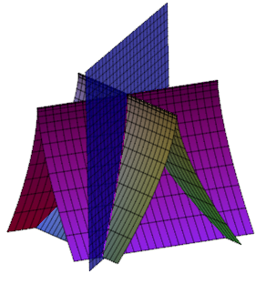
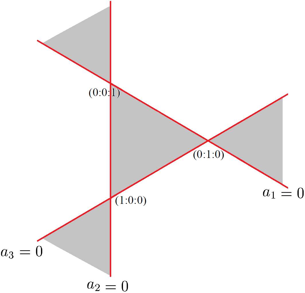
Figure 5: Left: The set $\mathcal{B}_{2}$ for $A_{1}^{2}A_{2}$. The $\mathcal{B}_{1}$ set (not shown) is the plane that contains both cuspidal edges of $\mathcal{B}_{2}$. Right: The regions determining the different types for $A_{1}^{2}A_{2}$.

Proposition 6.1

If $a_{1}a_{3}$ is positive the point $(a_{1}:a_{2}:a_{3})$ lies in the shaded region of Figure 5 (right) and the corresponding full bifurcation set has type $A_{1}A_{3}(a)$. If however $a_{1}a_{3}$ is negative, then the point lies in the unshaded region and the corresponding full bifurcation set is of type $A_{1}A_{3}(b)$.

Applying the chain rule to (1) in this case gives the system:

$$\left(\begin{array}[]{ccc}1&0&0\\ 0&0&0\\ 0&1&0\\ 0&0&1\end{array}\right)=\left.\left(\begin{array}[]{ccc}\frac{\partial^{2}F_{1}}{\partial t_{1}\partial u}&\frac{\partial^{2}F_{1}}{\partial t_{1}\partial x_{1}}&\frac{\partial^{2}F_{1}}{\partial t_{1}\partial x_{2}}\\ \frac{\partial F_{1}}{\partial u}&\frac{\partial F_{1}}{\partial x_{1}}&\frac{\partial F_{1}}{\partial x_{2}}\\ \frac{\partial F_{2}}{\partial u}&\frac{\partial F_{2}}{\partial x_{1}}&\frac{\partial F_{2}}{\partial x_{2}}\\ \frac{\partial F_{3}}{\partial u}&\frac{\partial F_{3}}{\partial x_{1}}&\frac{\partial F_{3}}{\partial x_{2}}\end{array}\right)\right|_{(A(t_{i},{\bf 0}),\mbox{\boldmath$x$}_{0})}\times JB+\left(\begin{array}[]{ccc}{\bf 0}\\ JC\\ JC\\ JC\end{array}\right).$$

Subtracting the second row from the third and fourth rows gives:

$$\left(\begin{array}[]{ccc}1&0&0\\ 0&0&0\\ 0&1&0\\ 0&0&1\end{array}\right)=\left.\left(\begin{array}[]{ccc}\frac{\partial^{2}F_{1}}{\partial t_{1}\partial u}&\frac{\partial^{2}F_{1}}{\partial t_{1}\partial v_{1}}&\frac{\partial^{2}F_{1}}{\partial t_{1}\partial v_{2}}\\ \frac{\partial F_{1}}{\partial u}&\frac{\partial F_{1}}{\partial x_{1}}&\frac{\partial F_{1}}{\partial x_{2}}\\ \frac{\partial F_{2}}{\partial u}-\frac{\partial F_{1}}{\partial u}&\frac{\partial F_{2}}{\partial x_{1}}-\frac{\partial F_{1}}{\partial v_{1}}&\frac{\partial F_{2}}{\partial x_{2}}-\frac{\partial F_{1}}{\partial x_{2}}\\ \frac{\partial F_{3}}{\partial u}-\frac{\partial F_{3}}{\partial u}&\frac{\partial F_{3}}{\partial x_{1}}-\frac{\partial F_{1}}{\partial x_{1}}&\frac{\partial F_{3}}{\partial x_{2}}-\frac{\partial F_{1}}{\partial x_{2}}\end{array}\right)\right|_{(A(t_{i},{\bf 0}),\mbox{\boldmath$x$}_{0})}\times JB+\left(\begin{array}[]{ccc}{\bf 0}\\ JC\\ {\bf 0}\\ {\bf 0}\end{array}\right).$$

Ignoring the second row and substituting the derivatives gives

$$\left(\begin{array}[]{ccc}1&0&0\\ 0&1&0\\ 0&0&1\end{array}\right)=\left.\left(\begin{array}[]{ccc}*&2\alpha_{1}X_{1}^{\prime}&-2\alpha_{1}Y_{1}^{\prime}\\ &\frac{2}{\kappa}(Y^{\prime}_{2}-Y^{\prime}_{1})&\frac{2}{\kappa}(X^{\prime}_{1}-X^{\prime}_{2})\\ &\frac{2}{\kappa}(Y^{\prime}_{3}-Y^{\prime}_{1})&\frac{2}{\kappa}(X^{\prime}_{1}-X^{\prime}_{3})\end{array}\right)\right|_{(A(t_{i},{\bf 0}),\mbox{\boldmath$x$}_{0})}\times JB.$$

Since the bifurcation type depends on whether $\frac{\partial B_{1}}{\partial a_{2}}\frac{\partial B_{1}}{\partial a_{3}}$ is positive or negative, evaluating these terms using the cofactors of the matrix gives

$$\frac{\partial B_{1}}{\partial a_{2}}{\frac{\partial B_{1}}{\partial a_{3}}} = \frac{16\alpha_{1}^{2}}{\kappa^{2}}(X_{1}^{\prime 2}-Y_{1}^{\prime 2}-X_{1}^{\prime}X_{2}^{\prime}+Y_{1}^{\prime}Y_{2}^{\prime})(X_{1}^{\prime}X_{3}^{\prime}-X_{1}^{\prime 2}+Y_{1}^{\prime 2}-Y_{1}^{\prime}Y_{3}^{\prime})$$ (15)

$$= -\frac{16\alpha_{1}^{2}}{\kappa^{2}}(\langle T_{1},T_{1}\rangle-\langle T_{1},T_{2}\rangle)(\langle T_{1},T_{1}\rangle-\langle T_{1},T_{3}\rangle).$$

$$= -\frac{16\alpha_{1}^{2}}{\kappa^{2}}((-1)^{\beta+1}-\langle T_{1},T_{2}\rangle)((-1)^{\beta+1}-\langle T_{1},T_{3}\rangle).$$

If the curves corresponding to the $A_{1}^{2}A_{2}$ point are spacelike, then the pseudo-circle is of type $S^{1}_{1}(c,r)$ (radius $r$ and centred at $c$) and can be parametrised as $S^{1}_{1}(\theta)=c+r(\cosh(\theta),\pm\sinh(\theta))$, where the $\pm$ allows for the covering of both branches. The unit tangent vectors at $\gamma_{i}$ are then given by $T_{i}=(\sinh(\theta_{i}),\pm\cosh(\theta_{i}))$. If both $\gamma_{1}$ and $\gamma_{i}$ ($i=2$ or $3$) lie on the same branch, then

$$\langle T_{1},T_{i}\rangle=-\sinh(\theta_{1})\sinh(\theta_{i})+\cosh(\theta_{1})\cosh(\theta_{i})=\cosh(\theta_{1}-\theta_{i})$$

so is greater than 1. If however $\gamma_{1}$ and $\gamma_{i}$ lie on opposite branches then

$$\langle T_{1},T_{i}\rangle=-\sinh(\theta_{1})\sinh(\theta_{i})-\cosh(\theta_{1})\cosh(\theta_{i})=-\cosh(\theta_{1}+\theta_{i})$$

so is less than $-1$. Since the curves $\gamma_{i}$ are locally spacelike, $\beta=1$ and the expression (15) is positive if $\gamma_{2}$ and $\gamma_{3}$, that is the two $A_{1}$ points, lie on the same branch and negative if they lie on opposite branches. It can be shown that the same result holds if the points are timelike. It follows that the point is of type $A_{1}^{2}A_{2}$ if of type $(a)$ if the two $A_{1}$ points lie on the same branch, and of type $(b)$ if they lie on opposite branches of the pseudo-circle.

7 The $A_{3}A_{1}$ singularity

Consider the following standard multi-versal unfolding of an $A_{3}A_{1}$ singularity given by

$$G:\mathbb{R}^{(2)}\times\mathbb{R}^{3}\to\mbox{$\mathbb{R}$}$$

where $\mathbb{R}^{(2)}$ denotes the parameters $t_{1},t_{2}$ and $\mathbb{R}^{3}$ denotes the unfolding parameters $\mbox{\boldmath$a$}=(a_{1},a_{2},a_{3})$ and the multi-versal unfolding is given by the two unfoldings:

$$G_{1}(t_{1},\mbox{\boldmath$a$}) = t_{1}^{4}+a_{1}t_{1}^{2}+a_{2}t_{1}+a_{3},$$

$$G_{2}(t_{2},\mbox{\boldmath$a$}) = t_{2}^{2}.$$

7.1 The big bifurcation set

At an $A_{3}A_{1}$ point the $\mathcal{B}_{2}$ set itself consists of two parts: The first is given as the solution to both $G_{1}=G_{2}$ and $G_{1}^{\prime}=G_{2}^{\prime}=0$ and is the swallowtail surface parametrised by $(a_{1},-4t_{1}^{3}-2a_{1}t_{1},3t_{1}^{4}+2t_{1}^{2}a_{1})$. The second component occurs locally near the $A_{3}$ point and is given by $G_{1}(t_{1})=G_{1}(-t_{1})$ and $G_{1}(t_{1})^{\prime}=G_{1}(-t_{1})^{\prime}=0$. This second component is the half plane $(-2t_{1}^{2},0,y_{3})$. The $\mathcal{B}_{1}$ component given by $G_{1}^{\prime}=G_{1}^{\prime\prime}=0$ is the semi-cubic cylinder $(-6t_{1}^{2},8t_{1}^{3},a_{3})$, (see Figure 6 (left)).

7.2 The bad planes

The adjacent singularities of codimension 1 are as follows:

$$A_{3} : \{(a_{1},a_{2},a_{3})=(0,0,a_{3})\}$$

$$A_{2}A_{1} : \{(a_{1},a_{2},a_{3})=(-6t_{1}^{2},8t_{1}^{3},-3t_{1}^{4})\}$$

$$A_{1}^{3} : \{(a_{1},a_{2},a_{3})=(-2t_{1}^{2},0,t_{1}^{4})\}$$

$$A_{1}^{2}/A_{1}^{2} : \{(a_{1},a_{2},a_{3})=(a_{1},0,0)\}$$

The limiting tangent vectors to these one-dimensional strata are given by $(1,0,0)$, and $(0,0,1)$ so the bad planes are given by $a_{1}=0$ and $a_{3}=0$.

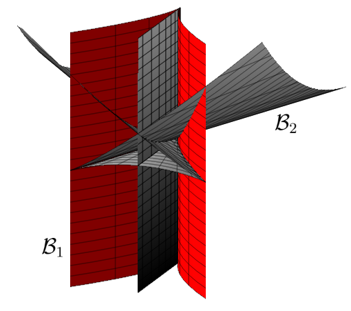
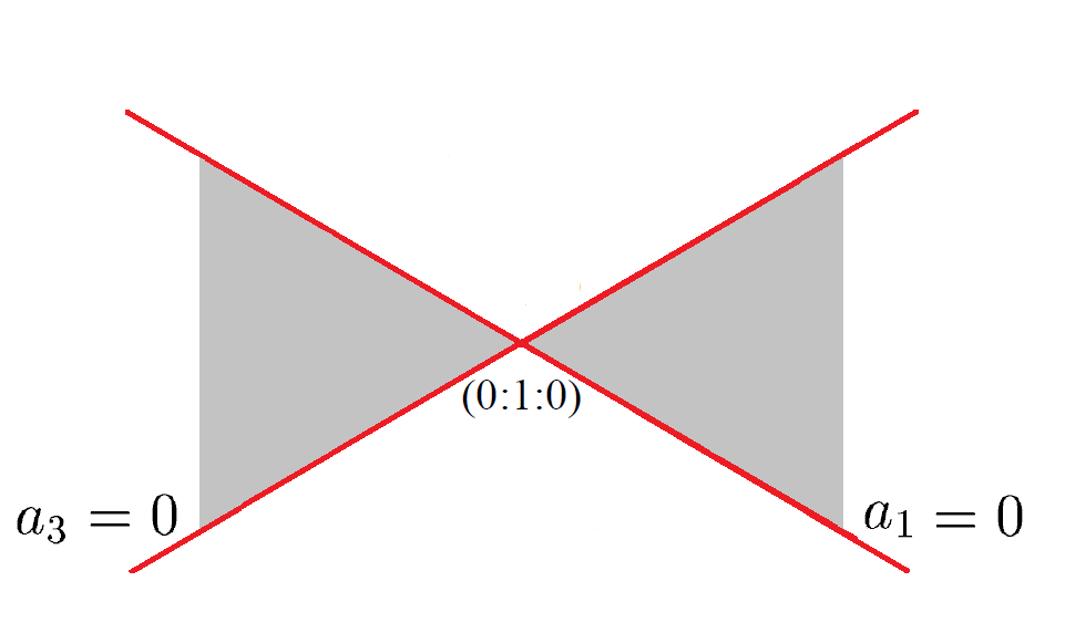
Figure 6: Left: The BBS for $A_{3}A_{1}$. Right: The regions determining the different types for $A_{3}A_{1}$.

Proposition 7.1

If $a_{1}a_{3}$ is positive the point $(a_{1}:a_{2}:a_{3})$ lies in the shaded region of Figure 6 (right) and the corresponding full bifurcation set has type $A_{1}A_{3}(a)$. If however $a_{1}a_{3}$ is negative, then the point lies in the unshaded region and the corresponding full bifurcation set is of type $A_{1}A_{3}(b)$.

Applying the chain rule to 1 gives the system:

$$\left(\begin{array}[]{ccc}1&0&0\\ 0&1&0\\ 0&0&1\\ 0&0&0\end{array}\right)=\left.\left(\begin{array}[]{ccc}\frac{\partial^{3}F_{1}}{\partial^{2}t_{1}\partial u}&\frac{\partial^{3}F_{1}}{\partial^{2}t_{1}\partial x_{1}}&\frac{\partial^{3}F_{1}}{\partial^{2}t_{1}\partial x_{2}}\\ \frac{\partial^{2}F_{1}}{\partial t_{1}\partial u}&\frac{\partial^{2}F_{1}}{\partial t_{1}\partial x_{1}}&\frac{\partial^{2}F_{1}}{\partial t_{1}\partial x_{2}}\\ \frac{\partial F_{1}}{\partial u}&\frac{\partial F_{1}}{\partial x_{1}}&\frac{\partial F_{1}}{\partial x_{2}}\\ \frac{\partial F_{2}}{\partial u}&\frac{\partial F_{2}}{\partial x_{1}}&\frac{\partial F_{2}}{\partial x_{2}}\end{array}\right)\right|_{(A(t_{i},{\bf 0}),\mbox{\boldmath$x$}_{0})}\times JB+\left(\begin{array}[]{ccc}{\bf 0}\\ {\bf 0}\\ JC\\ JC\end{array}\right).$$

Subtracting the last row from the third, and then ignoring the last gives:

$$\left(\begin{array}[]{ccc}1&0&0\\ 0&1&0\\ 0&0&1\end{array}\right)=\left.\left(\begin{array}[]{ccc}\frac{\partial^{3}F_{1}}{\partial^{2}t_{1}\partial u}&\frac{\partial^{3}F_{1}}{\partial^{2}t_{1}\partial x_{1}}&\frac{\partial^{3}F_{1}}{\partial^{2}t_{1}\partial x_{2}}\\ \frac{\partial^{2}F_{1}}{\partial t_{1}\partial u}&\frac{\partial^{2}F_{1}}{\partial t_{1}\partial x_{1}}&\frac{\partial^{2}F_{1}}{\partial t_{1}\partial x_{2}}\\ \frac{\partial F_{1}}{\partial u}-\frac{\partial F_{2}}{\partial u}&\frac{\partial F_{1}}{\partial x_{1}}-\frac{\partial F_{2}}{\partial x_{1}}&\frac{\partial F_{1}}{\partial x_{2}}-\frac{\partial F_{2}}{\partial x_{2}}\\ \end{array}\right)\right|_{(A(t_{i},{\bf 0}),\mbox{\boldmath$x$}_{0})}\times JB$$

Now,

$$\frac{\partial F_{i}}{\partial x_{1}}=2X_{i}-2x_{1},\frac{\partial F_{i}}{\partial x_{2}}=-2Y_{i}+2x_{2}$$

and $\gamma_{i}-\mbox{\boldmath$x$}=(X-x_{1},Y-x_{2})=\frac{1}{\kappa}N$ where $N=(-1)^{\beta}(Y_{1}^{\prime},X_{1}^{\prime})$. Hence, $\frac{\partial F_{i}}{\partial x_{1}}=2Y_{1}(-1)^{\beta}$ and $\frac{\partial F_{i}}{\partial x_{2}}=-2X_{1}^{\prime}(-1^{\beta})$. Substituting these derivatives into the matrix equation gives:

$$\left(\begin{array}[]{ccc}1&0&0\\ 0&1&0\\ 0&0&1\end{array}\right)=\left.\left(\begin{array}[]{ccc}*&2\alpha_{1}^{2}X_{1}^{\prime\prime}+4\alpha_{2}X_{1}^{\prime}&-2\alpha_{1}^{2}Y_{1}^{\prime\prime}-4\alpha_{2}Y_{1}^{\prime}\\ &2\alpha_{1}X_{1}^{\prime}&-2\alpha_{1}Y_{1}^{\prime}\\ &\frac{2}{\kappa}(-1)^{\beta}(Y^{\prime}_{1}-Y^{\prime}_{2})&\frac{2}{\kappa}(-1)^{\beta}(X^{\prime}_{2}-X^{\prime}_{1})\end{array}\right)\right|_{(A(t_{i},{\bf 0}),\mbox{\boldmath$x$}_{0})}\times JB.$$

Recall that the type of bifurcation depends upon whether $\frac{\partial B_{1}}{\partial a_{1}}\frac{\partial B_{1}}{\partial a_{3}}$ is positive or negative.

$$\frac{\partial B_{1}}{\partial a_{1}} = \ {\rm det}\left|\begin{array}[]{cc}2\alpha_{1}X_{1}^{\prime}&-2\alpha_{1}Y_{1}^{\prime}\\ \frac{2}{\kappa}(-1)^{\beta}(Y^{\prime}_{1}-Y^{\prime}_{2})&\frac{2}{\kappa}(-1)^{\beta}(X^{\prime}_{2}-X^{\prime}_{1})\end{array}\right|$$

$$= 2\alpha_{1}X_{1}^{\prime}\frac{2}{\kappa}(X^{\prime}_{2}-X^{\prime}_{1})+2\alpha_{1}Y_{1}^{\prime}\frac{2}{\kappa}(Y^{\prime}_{1}-Y^{\prime}_{2})$$

$$= \frac{4\alpha_{1}}{\kappa}(-X_{1}^{\prime 2}+Y_{1}^{\prime 2}+X_{1}^{\prime}X_{2}^{\prime}-Y_{1}^{\prime}Y_{2}^{\prime})$$

$$= \frac{4\alpha_{1}}{\kappa}(\langle T_{1},T_{1}\rangle-\langle T_{1},T_{2}\rangle).$$

and $\frac{\partial B_{1}}{\partial a_{3}}=-(2\alpha_{1}^{2}X_{1}^{\prime\prime}+4\alpha_{2}X_{1}^{\prime})2\alpha_{1}Y_{1}^{\prime}+2\alpha_{1}X_{1}^{\prime}(2\alpha_{1}^{2}Y_{1}^{\prime\prime}+4\alpha_{2}Y_{1}^{\prime})=4\alpha_{1}^{3}(X_{1}^{\prime}Y_{1}^{\prime\prime}-X_{1}^{\prime\prime}Y_{1}^{\prime})=4\alpha_{1}^{3}\kappa.$

$$\frac{\partial B_{1}}{\partial a_{1}}\frac{\partial B_{1}}{\partial a_{3}}=16\alpha_{1}^{4}(-1)^{\beta}(\langle T_{1},T_{1}\rangle-\langle T_{1},T_{2}\rangle).$$

So if $\gamma_{1}$ and $\gamma_{2}$ are both spacelike, this gives $16\alpha_{1}^{4}(1-\langle T_{1},T_{2}\rangle)$ which is negative if $\gamma_{1}$ and $\gamma_{2}$ lie on the same branch and positive if they lie on opposite branches (see Section 6). On the other hand, if they are both timelike this gives $-16\alpha_{1}^{4}(-1-\langle T_{1},T_{2}\rangle)$. Parametrising the psuedo-circle of type $H^{1}(c,-r)$ as $H^{1}(\theta)=c+r(\pm\sinh(\theta),\cosh(\theta))$, the unit tangent vector is given by $T=(\pm\cosh(\theta),\sinh(\theta))$. Now if $\gamma_{1}$ and $\gamma_{2}$ lie on the same branch $\langle T_{1},T_{2}\rangle=-\cosh(\theta_{1})\cosh(\theta_{2})+\sinh(\theta_{1})\sinh(\theta_{2})=-\cosh(\theta_{1}-\theta_{2})$ which is less than -1. However if $\gamma_{1}$ and $\gamma_{2}$ lie on opposite branches $\langle T_{1},T_{2}\rangle=\cosh(\theta_{1})\cosh(\theta_{2})+\sinh(\theta_{1})\sinh(\theta_{2})=\cosh(\theta_{1}+\theta_{2})$ which is greater than 1. Hence the expression $-16\alpha_{1}^{4}(-1-\langle T_{1},T_{2}\rangle)$ is negative if $\gamma_{1}$ and $\gamma_{2}$ lie on the same branch and positive if they lie on opposite branches (the same conditions as for spacelike). It follows that the type is $A_{1}A_{3}(a)$ if both contact points lie on opposite branches and type $A_{1}A_{3}(b)$ occur on the same branch of the pseudo-circle.

8 The $A_{4}$ singularity

Consider the following standard versal unfolding of an $A_{4}$ singularity given by

$$G:\mathbb{R}\times\mathbb{R}^{3}\to\mbox{$\mathbb{R}$}$$

where $\mathbb{R}$ denotes the parameters $t$ and $\mathbb{R}^{3}$ denotes the unfolding parameters $\mbox{\boldmath$a$}=(a_{1},a_{2},a_{3})$ and the versal unfolding is given by the two unfoldings:

$$G(t,\mbox{\boldmath$a$}) = t^{5}+a_{1}t^{3}+a_{2}t^{2}+a_{3}t.$$

8.1 The big bifurcation set

The bifurcation set $\mathcal{B}_{1}$ of the standard $A_{4}$ singularity $G$ is the swallowtail surface which can be parametrised by $(a_{1},-10t^{3}-3a_{1}t)$, and its bifurcation set $\mathcal{B}_{2}$ is another swallowtail, which sits inside the swallowtail $\mathcal{B}_{1}$ and can be parametrised by $(-3s^{2}-4st-3t^{2},2s^{3}+8s^{2}t+8st^{2}+2t^{3},-4s^{3}t-7s^{2}t^{2}-4st^{3})$. See Figure 7. The adjacent 1-dimensional strata are found to be

$$A_{3} : \{(a_{1},a_{2},a_{3})=(-10t^{2},20t^{3},-15t^{4})\}$$

$$A_{1}A_{2} : \{(a_{1},a_{2},a_{3})=(-60t^{2},-80t^{3},960t^{4})\}$$

$$A_{2}/A_{2} : \{(a_{1},a_{2},a_{3})=(-\frac{10}{3}t^{2},0,5t^{4})\}$$

$$A_{1}^{2}/A_{1}^{2} : \{(a_{1},a_{2},a_{3})=(-4t^{2},0,\frac{16}{5}t^{4})\}.$$

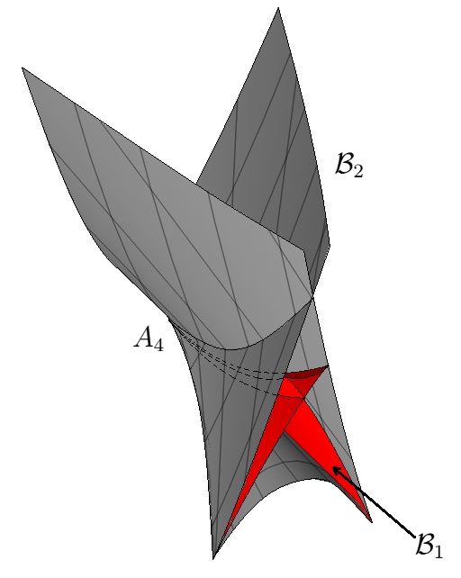
Figure 7: The BBS for $A_{4}$.

The limiting tangent vectors to these one-dimensional strata are all given by $(1,0,0)$, so the only bad planes is given by $a_{1}=0$. Examining representations from both components show that only transition type exists for $A_{4}$.

References

- [1] H. Blum, ‘A transformation for extracting new descriptors of shape’. W. Whaten-Dunn (Ed.), Models for the perception of speech and visual forms, MIT Press, Cambridge, MA, (1967), 362-380.
- [2] J.W. Bruce, ‘Generic functions on semi-algebraic sets’, Quart. J. Math Oxford 37 (2), (1986), 137-165.
- [3] J.W. Bruce and P.J. Giblin, ‘Growth, motion and 1-parameter families of symmetry sets’, Proc. Roy. Soc. of Edin., 104A (1986), 179-204.
- [4] J.W. Bruce, P.J. Giblin and C.G. Gibson, ‘Symmetry sets’, Proc. of the Royal Soc.of Edinburgh, 101A, (1985), 163-186.
- [5] P.J. Giblin and S.A. Brassett, ‘Local symmetry of plane curves’, Amer. Math. Monthly 92 (1985), 689–707.
- [6] P.J. Giblin and P.A. Holtom, ‘Affine-distance symmetry sets’, Mathematica Scandanavica 93(2), (2003), 247-267.
- [7] P.J. Giblin and B.B. Kimia, ’On the local form and transitions of symmetry sets, medial axes and shocks’, International Journal of Computer Vision, 54 (1/2/3), (2003), 143-158.
- [8] P.A. Holtom, ‘Affine-invariant symmetry sets’, PhD Thesis, University of Liverpool (2000).
- [9] A.J. Pollitt ‘Euclidean and affine symmetry sets and medial axes’, PhD Thesis, University of Liverpool (2004).
- [10] G.M. Reeve and F. Tari, ‘Minkowski symmetry sets of plane curves’, Proceedings of the Edinburgh Mathematical Society, 60(2), (2016), 461-480.
- [11] G.M. Reeve and F. Tari, ‘Minkowski medial axes and shocks’, The AMS Mathematics Series, 675 (2016) 263-278.
- [12] K. Siddiqi and M. Pizer, Medial Representations: Mathematics, Algorithms and Applications. Springer (2008).
- [13] A. Saloom and F. Tari, ‘Curves in the Minkowski plane and their contact with pseudo-circles’, Geom. Dedicata 159, (2012), 109-124.