Vacuum effects on the properties of nuclear matter under an external magnetic field

Abstract

The effects of the Dirac sea of the nucleons are investigated within a covariant model of the hadronic interaction. I extend the usual Mean Field Approximation and present a procedure to deal with divergences which are proportional to polynomials on the magnetic field intensity. For this purpose a nucleon propagator is used which takes account of the full effect of the magnetic field as well as the presence of the anomalous magnetic moments of both protons and neutrons. I examine single-particle properties and bulk thermodynamical quantities and conclude that within a reasonable range of densities and magnetic intensities the effects found are moderate.

1 Introduction

The interaction between matter and strong magnetic fields is a subject of permanent research [1, 2]. In particular the combination of magnetic fields and the strong interaction has been intensively debated in the low [3, 4, 5, 6, 7, 8, 9, 10, 11, 12] and medium energy regimes [13, 14, 15, 16, 17]. In the first case, the use of hadronic degrees of freedom is indispensable. Among the most used models of the hadronic interaction, the Quantum Hadro-Dynamics(QHD) has a remarkable versatility to describe a variety of phenomena and its results have a satisfactory accuracy when it is required.
QHD has been used to study the interaction of hadrons and magnetics fields, for instance in the structure and composition of neutron stars [3, 4, 5],the liquid-gas phase transition [6], the neutrino propagation in nuclear matter [7], the deconfinement phase transition [8], magnetic catalysis [9, 10], the modification of nuclear structure [11], and the formation of magnetic domains [12].
Within this description there is a general agreement that the anomalous magnetic moments (AMM) of the hadrons play a significative role when the magnetic energy approaches the QCD scale, i.e. $qB\approx(220MeV)^{2}$ [4, 5, 7, 10].
One of the features of the QHD models is the simplicity of conceptual resources and procedures. The crucial point for these models is the Mean Field Approximation (MFA) where the meson fields are replaced by their in medium-mean values. In addition, the bilinear products of fermion fields are replaced by their expectation values. In the last case the contributions coming from the Dirac sea of fermions are usually disregarded. The procedure is completed with the requirement of self-consistency of the scalar meson fields, which are not directly related to conserved charges.
The same procedure was adopted for a model based on the chiral SU(3) symmetry of the strong interaction [18], which was used to study different aspects of hadronic matter subject to an external magnetic field [19, 20, 21].
Some attempts has been made to incorporate the vacuum contribution within this scheme [9, 10]. However, in [9] the AMM of the nucleons are neglected, although very strong magnetic intensities are considered ($q\,B\approx(500MeV)^{2}$). Furthermore, there is no contribution of the neutron.
On the other hand, in [10] a low magnetic intensity expansion is proposed for the nucleon propagator, where the discrete energy spectrum of the protons due to the Landau quantization is not taken into account.
The technical difficulties arising when the vacuum contributions in the presence of an external magnetic field are included have recently been considered within the Nambu and Jona-Lasinio model of the quark interaction [16].

An analysis of the magnitude of the vacuum effects under the influence of strong magnetic fields, taking into account all the physical ingredients in a coherent manner, is necessary to discuss the validity of the usual MFA.
This is precisely the aim of the present work. Here a version of the QHD model with polynomial meson interactions is used; it is known as FSUGold [22]. Contributions of the vacuum are evaluated by using a nucleon propagator which includes the anomalous magnetic moments and the full interaction with the external magnetic field [23, 24]. This propagator has been used to evaluate meson properties [20, 24] and the effect of the AMM within the Nambu and Jona-Lasinio model [17].
Within this scheme I evaluate the effective nucleon mass and statistical properties such as the grand canonical potential and the magnetization as functions of the baryonic density and the magnetic intensity at zero temperature.

This work is organized as follows. In the next section the QHD prescriptions for the MFA as well as its extension to include the vacuum contributions are presented. Some numerical results are discussed in Sec. III, and the last section is devoted to drawing the conclusions of this work.

2 Vacuum corrections to the MFA within the QHD model

The field equations for the QHD model supplemented with the couplings of an external magnetic field to the charge of the proton, as well as to the anomalous magnetic moments of both protons and neutrons, are [4]

$$\left(i\,\not\!\partial-m+g_{s}\sigma+q_{b}\not\!\!A-g_{w}\not\!\omega-g_{r}\bm{\tau\cdot}\not\!\!\bm{\rho}-\kappa_{b}\,\sigma_{\mu\nu}F^{\mu\nu}\right)\Psi_{b}=0$$ (1)

$$\left(\square+m_{s}^{2}+g_{s2}\,\sigma+g_{s3}\,\sigma^{2}\right)\sigma=g_{s}\sum_{b}\bar{\Psi}_{b}\Psi_{b}$$ (2)

$$\partial_{\mu}\Omega^{\mu\nu}+\left(m_{w}^{2}+G_{w}\omega_{\mu}\omega^{\mu}+G_{rw}\bm{\rho}_{\mu}{\bm{\cdot}}\bm{\rho}^{\mu}\right)\omega^{\nu}=g_{w}\sum_{b}\bar{\Psi}_{b}\gamma^{\nu}\Psi_{b}$$ (3)

$$D_{\mu}R_{a}^{\mu\nu}+\left(m_{r}^{2}+G_{rw}\omega_{\mu}\omega^{\mu}\right)\rho_{a}^{\nu}=g_{r}\sum_{bc}\bar{\Psi}_{b}\tau^{(a)}_{bc}\gamma^{\nu}\Psi_{c}$$ (4)

where the index $b$ in Eq. (1) indicates proton or neutron, $\Omega_{\mu\nu}$ and $R_{\mu\nu}$ are the field tensors for the $\omega$ and $\rho$ fields, and the couplings constants are related to the notation of [22] by $g_{s}=g_{\sigma N}$, $g_{s2}=\kappa\,g_{\sigma N}^{3}/2$, $g_{s3}=\lambda\,g_{\sigma N}^{4}/6$, $G_{w}=\zeta\,g_{\omega N}^{4}/6$, and $G_{rw}=2\,\Lambda_{w}g_{rN}^{2}g_{wN}^{2}$.

Assuming uniform matter distribution, the meson fields in these equations are replaced by functions depending only on the bulk properties of the system. Furthermore, the products of fermionic fields on the right-hand side of Eqs. (2), (3), and (4) are replaced by their expectation values. Under such conditions, and adopting the reference frame of rest matter, only the cases with $\nu=0$ gives non-zero values in Eqs. (3) and (4). Finally, as the weak decay is not contemplated in the interaction, only the case $a=3$ in Eq. (4) gives a non-zero contribution.
The above mentioned expectation values can be evaluated by using the appropriate fermion propagators

$${\cal N}_{s\,b}= <\bar{\Psi}_{b}\,\Psi_{b}> =-i\;\lim_{t^{\prime}\rightarrow t^{+}}\,\text{Tr}\{G_{b}(t,\vec{r},t^{\prime},\vec{r})\}$$ (5)

$${\cal N}^{\nu}_{b}= <\bar{\Psi}_{b}\,\gamma^{\nu}\,\Psi_{b}> =-i\;\lim_{t^{\prime}\rightarrow t^{+}}\,\text{Tr}\{\gamma^{\nu}\,G_{b}(t,\vec{r},t^{\prime},\vec{r})\}$$ (6)

In the momentum representation they can be rewritten as

$${\cal N}_{s\,b} = -i\;\lim_{\epsilon\rightarrow 0^{+}}\,\int\frac{d^{4}p}{(2\pi)^{4}}e^{-ip_{0}\epsilon}\;\text{Tr}\{G_{b}(p)\}$$ (7)

$${\cal N}^{\nu}_{b} = -i\;\lim_{\epsilon\rightarrow 0^{+}}\,\int\frac{d^{4}p}{(2\pi)^{4}}e^{-ip_{0}\epsilon}\;\text{Tr}\{\gamma^{\nu}G_{b}(p)\}$$ (8)

In [23] a fermion propagator which includes the full interaction with the external magnetic field, through its coupling to the proton charge and to the AMM also, was used for this purpose. For the sake of completeness the explicit form of the neutron propagator is

$$G_{n}(x^{\prime},x)=\sum_{s}\int\frac{d^{4}p}{(2\pi)^{4}}e^{-ip^{\mu}\,(x_{\mu}^{\prime}-x_{\mu})}\Lambda_{s}\;\Xi_{p}$$ (9)

where

$$\Lambda_{s} = \frac{s}{2\Delta}i\;\gamma^{1}\gamma^{2}\left[\not\!u+i\gamma^{1}\gamma^{2}(s\Delta-\kappa B)\right]\left(\not\!v+m+is\Delta\gamma^{1}\gamma^{2}\right)$$ (10)

$$\Xi_{p} = \frac{1}{p_{0}^{2}-E_{s}^{2}+i\epsilon}+2\pi\,i\,n_{F}(p_{0})\,\delta(p_{0}^{2}-E_{s}^{2})$$ (11)

whereas for the proton one has

$$G_{p}(x^{\prime},x)=e^{i\Phi}\int\frac{d^{4}p}{(2\pi)^{4}}e^{-ip^{\mu}\,(x^{\prime}_{\mu}-x_{\mu})}\left[G_{0}(p)+e^{-p_{\bot}^{2}/\beta}\sum_{n,s}(-1)^{n}G_{n,s}(p)\right]$$ (12)

where

$$G_{0}(p) = 2e^{-p_{\bot}^{2}/\beta}\Lambda^{0}\;\Xi_{0\,1}$$ (13)

$$G_{ns}(p) = \frac{\Delta_{n}+sm}{2\Delta_{n}}\Big{\{}(\not\!u-\kappa_{p}B+s\Delta_{n})\left(1+i\gamma^{1}\gamma^{2}\right)L_{n}(2p_{\bot}^{2}/\beta)-(\not\!u+\kappa_{p}B-s\Delta_{n})$$ (14)

$$\times\left(1-i\gamma^{1}\gamma^{2}\right)\frac{s\Delta_{n}-m}{s\Delta_{n}+m}L_{n-1}(2p_{\bot}^{2}/\beta)+\left(\not\!u\,i\gamma^{1}\gamma^{2}+s\Delta_{n}-\kappa_{p}B\right)\not\!v\frac{s\Delta_{n}-m}{p_{\bot}^{2}}$$

$$\times\left[L_{n}(2p_{\bot}^{2}/\beta)-L_{n-1}(2p_{\bot}^{2}/\beta)\right]\Big{\}}\;\Xi_{ns}$$

$$\Xi_{ns} = \frac{1}{p_{0}^{2}-E_{ns}^{2}+i\epsilon}+2\pi\,i\,n_{F}(p_{0})\,\delta(p_{0}^{2}-E_{ns}^{2})$$ (15)

In these expressions the index $s=\pm 1$ corresponds to the projection of the spin in the direction of the uniform magnetic field, the index $n\geq 1$ takes account of the discrete Landau levels, and the following notation is used: $\beta=qB$, $\not\!u=p_{0}\gamma^{0}-p_{z}\gamma^{3}$, $\not\!v=-p_{x}\,\gamma^{1}-p_{y}\,\gamma^{2}$, $p_{\bot}^{2}=p_{x}^{2}+p_{y}^{2}$, $L_{m}$ stands for the Laguerre polynomial of order $m$, and

$$E_{s} = \sqrt{p_{z}^{2}+(\Delta-s\,\kappa_{n}B)^{2}}$$

$$\Delta = \sqrt{m^{2}+p^{2}_{x}+p^{2}_{y}}$$

$$E_{ns} = \sqrt{p_{z}^{2}+(\Delta_{n}-s\,\kappa_{p}B)^{2}}$$

$$\Delta_{n} = \sqrt{m^{2}+2nqB}$$

Finally, the phase factor $\Phi=qB(x+x^{\prime})(y^{\prime}-y)/2$ embodies the gauge fixing.

If these propagators are used in Eqs. (7) and (8), but keeping only the second terms of Eqs. (11) and (15), then the MFA is obtained [23]. The correction to the densities coming from the Dirac sea of nucleons can be evaluated by using Eqs. (7) and (8) but retaining only the first terms of Eqs. (11) and (15). The expressions thus obtained are divergent and must be renormalized. Since the main residue in a Lorenz expansion depends on the magnetic intensity, a regularization procedure must be defined to extract relevant contributions. The details of this calculations are left for the Appendix, and here the final results are shown. ${\cal N}_{\nu}^{\text{vac}}=0$ for protons and neutrons,

$${\cal N}_{s\,p}^{\text{reg}} = \frac{1}{4\pi^{2}}\Big{[}2\beta\kappa_{p}B+\frac{\beta^{2}}{3m}-m^{3}+2\beta(m+\kappa_{p}B)\ln\left(\frac{m}{m+\kappa_{p}B}\right)$$ (16)

$$+m\left(\beta-m^{2}\right)\ln\left(\frac{2\beta}{m^{2}}\right)-2m\beta\ln\left(\frac{\Gamma(m^{2}/2\beta)}{\sqrt{2\pi}}\right)\Big{]}$$

for protons, and

$${\cal N}_{s\,n}^{\text{reg}}=\frac{m}{4\pi^{2}}\left[6(\kappa_{n}B)^{2}+(m-\kappa_{n}B)^{2}\ln\left(\frac{m}{m-\kappa_{n}B}\right)+(m+\kappa_{n}B)^{2}\ln\left(\frac{m}{m+\kappa_{n}B}\right)\right]$$ (17)

for neutrons.
It must be pointed out that the first three terms on the right-hand side of Eq. (16) come from the subtraction proposed in the regularization procedure. It is interesting to note that Eq.(17) becomes zero if $\kappa_{n}=0$ is taken, while, taking $\kappa_{p}=0$ in Eq. (16) and writing $x=m^{2}/2\beta$, this equation reduces to

$$-\frac{m\beta}{2\pi^{2}}\Big{[}-\frac{1}{12x}+x-x\ln(x)+\frac{1}{2}\ln\left(\frac{x}{2\pi}\right)+\ln\left(\Gamma(x)\right)\Big{]}.$$ (18)

Here the first two terms correspond to the second and third terms of (16). With exception of the first term between square brackets in Eq.(18), this expression can be recognized as the vacuum correction term on the right-hand side of Eq. (28a) of Ref. [9]. As explained before, the discrepant term is justified by the subtraction prescription used here.

With these results, one can extend the standard definition of the effective nucleon mass in QHD models $m=m_{0}-g_{s}\,\bar{\sigma}$, where $m_{0}=939$ MeV and the uniform mean value $\bar{\sigma}$ is obtained from Eq.(2) by neglecting the coordinate dependence and replacing $\bar{\Psi}_{b}\Psi_{b}\rightarrow{\cal N}_{s\,b}$. And the scalar baryonic density is the sum of the MFA result and the vacuum correction given by Eqs. (16) and (17). The self-consistency is imposed by evaluating ${\cal N}_{s\,b}$ in the unknown mass $m$.

For further applications it is useful to obtain the vacuum correction to the energy density. The baryonic contribution to the energy density arises from the mean field value of the Hamiltonian density operator [23]

$${\cal E}_{b}=<{\cal H}_{b}>=-i\;\lim_{t^{\prime}\rightarrow t^{+}}\,\text{Tr}\left\{i\gamma^{0}\frac{\partial}{\partial t}\,G_{b}(t,\vec{r},t^{\prime},\vec{r})\right\}.$$ (19)

By using the method described in the Appendix, the following results are obtained:

$${\cal E}_{n}^{\text{reg}} = \frac{1}{48\pi^{2}}\Big{\{}\left[(\kappa_{n}B)^{4}-6m^{2}(\kappa_{n}B)^{2}-3m^{4}\right]\ln\left[\frac{m^{2}-(\kappa_{n}B)^{2}}{m^{2}}\right]-4\kappa_{n}Bm^{3}\ln\left(\frac{m+\kappa_{n}B}{m-\kappa_{n}B}\right)$$ (20)

$$+\frac{13}{6}(\kappa_{n}B)^{2}\left[6m^{2}-(\kappa_{n}B)^{2}\right]\Big{\}}$$

$${\cal E}_{p}^{\text{reg}} = \frac{1}{8\pi^{2}}\Big{\{}-4\beta^{2}\zeta^{\prime}(-1,\lambda)-\frac{1}{2}\ln\left(\frac{m^{2}}{2\beta}\right)\left(\mu^{2}-2\beta\mu+\frac{2}{3}\beta^{2}\right)-\frac{1}{4}m^{4}+\left[\beta+(\kappa_{p}B)^{2}\right]^{2}$$ (21)

$$-2\beta(m+\kappa_{p}B)^{2}\ln\left(\frac{m+\kappa_{p}B}{m}\right)+\frac{1}{3}\beta(\beta+2m\kappa_{p}B)\left(\frac{\kappa_{p}B}{m}\right)^{2}-\frac{2}{3}\beta^{2}+2m\beta\kappa_{p}B$$

$$+\frac{1}{45}\left(\frac{\beta}{m}\right)^{4}\Big{\}}$$

where $m$ stands for the vacuum value, i.e., $m=m_{0}$, $\mu=m_{0}^{2}+(\kappa_{p}B)^{2}$, $\lambda=\mu/2\beta$, and $\zeta^{\prime}$ indicates the derivative of the Hurwitz zeta function respect to its first argument.
The magnetization of the system can be evaluated as ${\cal M}=\left(\partial{\cal E}/\partial B\right)_{N_{b}}$, where ${\cal E}$ is the hadronic contribution to the total energy [4]. Finally, using the chemical potentials associated with the conservation of the baryonic number of protons and neutrons, the pressure at zero temperature can be evaluated as $P=\sum_{b}\mu_{b}n_{b}-{\cal E}$.

3 Results and discussion

In this section several properties of dense nuclear matter are analyzed, considering baryonic densities lesser than three times the normal nuclear density and magnetic intensities between $10^{14}$ and $10^{19}$ G. The isospin composition of matter has also been taken as a relevant variable to be examined. However, the main conclusions of this work are basically independent of the isospin asymmetry, so I examine in what follows the symmetric nuclear matter case.
The parameters are taken from the FSU model [22].

First the effective nucleon mass is analyzed. It is directly affected by the vacuum corrections to the scalar densities given by Eq. (7). In Fig. 1 the dependence of $m$ on the magnetic intensity is displayed at constant baryonic density. For this purpose I take $n/n_{0}=0,\,1,\,2$, where $n_{0}$ stands for the normal nuclear density. In each case the results including vacuum correction (CC) and without it (NC) are compared. For intensities below $5\times 10^{18}$ G, both cases yields very similar results. Up to this point, the inclusion of corrections produces higher values of the effective mass. This effect is more pronounced at lower densities, for instance at $B=10^{19}$ G the differences between the two cases are 2.7, 2.2, and 1.9 MeV for the densities $n/n_{0}=0,\,1,\,2$ respectively. This can be understood because the vacuum effect at fixed magnetic intensity reduces to a constant which dominates at very low densities. But, as the density increases, the MFA provides a growing contribution.
In Fig. 1 a wider range of magnetic intensities is considered in order to compare with previous results. For instance in [9] the difference for the nucleon mass between the CC and NC cases at zero density is approximately $10$ and $20$ MeV for $B=10^{19}$ and $1.6\times 10^{19}$ G, respectively, whereas in these calculations I have obtained $3$ MeV and $9$ MeV for the same values of the magnetic intensity. This fact is illustrated in Fig. 2a, where the results of the present work (solid line) are contrasted with those obtained by following the procedure and model parameters used in [9] (dotted line). In order to expand the analysis, I also show the results obtained with the FSU model including the AMM but adopting the regularization procedure of Ref.[9] (dash-dotted line). I conclude that the numerical discrepancy comes mainly from the different regularization prescriptions and in a minor degree can be ascribed to the model parameters and to the presence of the AMM. Notwithstanding, even for the extreme intensity $B=10^{19}$ G, all the approaches predict an increment of the effective mass not greater than $2\%$ of the experimental value $m_{0}$.
The role of the anomalous magnetic moments is analyzed throughout the three panels of Fig. 2. The outcome for the present calculations with $\kappa_{p}=\kappa_{n}=0$ at fixed density is represented by the curves with dashed lines. Neglecting the AMM yields a decreasing effective mass, that increasingly differs from the full calculations as the magnetic intensity and the baryonic density are increased. For a given density and low intensities ($B<10^{18}$ G) the results with or without AMM are almost identical, whereas for the greatest intensity examined here ($B=1,6\times 10^{19}$ G) the difference grows from $10$ to $25$ MeV.

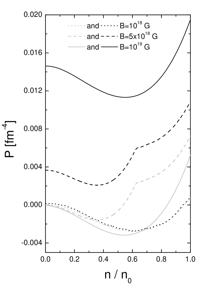
Figure 3: The pressure as a function of the baryonic density for several magnetic intensities. A comparison of the results with and without vacuum correction is included according to the line convention shown in this figure.

As the next step, the pressure at zero temperature is studied. In Fig.3 the pressure as a function of the particle density is shown for a constant magnetic intensity, for the specific values $B=10^{18},\,5\times 10^{18}$ and $10^{19}$ G. Again a comparison between the CC and NC cases is made. For each pair of curves the CC case presents higher values for the whole range of densities. Furthermore the separation between each pair does not vary significatively with the density. This can be explained because the vacuum correction does not depend on the density, and the changes induced in the meson mean values are so weak that the CC curve practically copies the same features of the NC one. However the shift between the twin curves increases appreciably with the magnitude of $B$. This behavior remains when the isospin composition is varied.
An interesting consequence which can be appreciated in Fig. 3, is that the vacuum correction preserves the thermodynamical instabilities of the MFA. Therefore a spinodal decomposition similar to that shown in [6] must be expected, with the same range of densities but extending to higher pressures.
It must be said that in order to allow an easier comparison within the same figure, the constant contribution of the magnetic field to the total energy density is not shown in Fig. 3.

As the last statistical subject to be analyzed the magnetization ${\cal M}$ induced by the external magnetic field is considered. It must be mentioned that within the scheme of regularization presented here, one can obtain finite vacuum contributions to ${\cal M}$ as also would be the case for the magnetic susceptibility $\chi=\partial{\cal M}/\partial B$.
It is known that ${\cal M}$ is a very weak quantity, since it is proportional to the electric charge. The correction to the energy density, given by Eqs. (20) and (21), does not depend on the matter density, nor does its contribution to the magnetization. Hence I analyze the dependence on $B$ of the difference $\Delta{\cal M}$ between the full magnetization and the corresponding result without vacuum effect. To compare with previous calculations [5, 25] which used the same hadronic interaction, the adimensional ratio $\Delta{\cal M}/q^{2}B$ as a function of the magnetic intensity is shown in Fig. 4, separately for the proton and neutron contributions within the range $10^{17}$ $<B<10^{19}$ G. By considering the results of [25] for $B>10^{18}$ G, an almost general trend is that this quantity decreases by increasing the magnetic intensity and decreasing the matter density. Due to the tiny results I obtained for the neutron component, one can expect that the vacuum corrections to this component could have significative effects only in the very low density regime. However, in this regime the assumption of homogeneous matter is not valid. So, one can conclude that the vacuum correction to the neutron component is negligible, with the possible exception of certain special configurations, for instance, in the case of the neutron gas surrounding the nuclear clusters in the inner crust of a neutron star.
In regard to the proton component, a growing magnitude is obtained as $B$ is increased, reaching at $B=10^{19}$ G the value $10^{-5}$. This represents approximately $10\%$ of the result at a density $n/n_{0}=0.2$ (see Fig. 8 of Ref. [25]) and $1\%$ at $n/n_{0}=1.2$. In conclusion, the vacuum correction for the proton component starts to be significant for intensities $B\approx 10^{19}$ G, modifying the MFA result only by a few percent for densities below the normal nuclear density.

4 Conclusions

In this work I have proposed an extension of the MFA for nuclear matter under the effect of a uniform magnetic field, by including contributions from the Dirac sea of hadrons. I have used the covariant FSU model of the nuclear interaction [22] and the calculations have been made by using a covariant propagator which takes account of the full effect of the magnetic field as well as the effect of the anomalous magnetic moments. Hence, several issues left open in previous investigations [9, 10] are considered.

Since the interaction used is just an effective model of the strong interaction, I have not considered a renormalization scheme. In particular I did not try to renormalize the external magnetic field since, within the model used, it is not a dynamical variable. I have proposed instead a regularization procedure to obtain physically meaningful results from the divergent contributions.
The procedure has the advantage of yielding finite results for the vacuum correction to the magnetization ${\cal M}=\partial{\cal E}/\partial B$ as well as to the higher order derivatives, for instance the magnetic susceptibility $\chi=\partial{\cal M}/\partial B$.

Within the scheme proposed I have evaluated different nuclear properties at zero temperature. The effective nucleon mass is representative of the single-particle properties, and the pressure and the magnetization correspond to bulk properties in thermodynamical equilibrium. They have been analyzed for a range of matter densities and magnetic intensities that ensures the confidence in the model.
For all the cases I have obtained moderate corrections, which becomes significant for densities below the normal nuclear density, and magnetic intensities above $10^{18}$ G.
Taking into account that QHD models use hadronic degrees of freedom exclusively and that their parameters are adjusted to the low energy phenomenology, it is consistent that vacuum corrections do not reveal high energy manifestations. These conclusions support the validity of the MFA for the regime of parameters studied.

5 Acknowledgements

This work has been partially supported by a grant from the Consejo Nacional de Investigaciones Cientificas y Tecnicas, Argentina.

Appendix A Regularization of the vacuum contribution to the nuclear densities

I start with the nuclear current (8). By using the vacuum component of either Eq.(9) or Eq. (12), it is found that the integrand of Eq. (8) is odd in the integration variables, hence, by symmetric integration it is zero for all $\nu$.

Next, the neutron scalar density Eq.(7) is considered. Using the neutron propagator, one finds for the vacuum term

$${\cal N}_{s\,n}^{\text{vac}} = -\frac{2\,i}{(2\,\pi)^{4}}\frac{m}{\nu}\,\sum_{s}\int\;d^{4}p\;\frac{\Delta-s\kappa_{n}B}{\Delta}\,\frac{\nu}{u_{p}^{2}-(\Delta-s\kappa_{n}B)^{2}+i\varepsilon}$$ (22)

where a regularization parameter $\nu$ with dimension of squared mass has been introduced. After passing to a bidimensional Euclidean space in the variables $p_{0}$ and $p_{z}$, this can be written as

$$\frac{-2}{(2\,\pi)^{4}}\frac{m}{\nu}\,\sum_{s}\int_{0}^{\infty}d\tau\int\,d^{2}p_{\bot}\frac{\Delta-s\kappa_{n}B}{\Delta}\,\exp\left[-\tau(\Delta-s\kappa_{n}B)^{2}/\nu\right]\int d^{2}p_{E}\;e^{-\tau p_{E}^{2}/\nu}$$ (23)

After performing the momentum integrals, one obtains

$$-\frac{m\,\nu}{8\pi^{2}}\lim_{\epsilon\rightarrow 0}\sum_{s}\int_{0}^{\infty}d\tau\;\tau^{\epsilon-2}e^{-\tau(m-s\kappa_{n}B)^{2}/\nu}$$ (24)

which by the change of variable $t=\tau(m-s\kappa_{n}B)^{2}/\nu$, takes the form

$$-\frac{m}{8\pi^{2}}\lim_{\epsilon\rightarrow 0}\Gamma(\epsilon-1)\;\sum_{s}(m-s\kappa_{n}B)^{2}\left[\frac{(m-s\kappa_{n}B)^{2}}{\nu}\right]^{-\epsilon}$$ (25)

Here a single pole can be distinguished from the finite contributions

$$\frac{m}{8\pi^{2}}\lim_{\epsilon\rightarrow 0}\left\{\left(\frac{1}{\epsilon}+1-\gamma\right)2\left(m^{2}+\kappa_{n}^{2}B^{2}\right)-\sum_{s}\left(m-s\kappa_{n}B\right)\log\left[\frac{(m-s\kappa_{n}B)^{2}}{\nu}\right]+{\cal O}(\epsilon)\right\}$$ (26)

when $B\rightarrow 0$ this expression reduces to the standard result, obtained for instance by dimensional regularization from the Feynman propagator.
The residue of this pole depends quadratically on $B$, hence I propose a regularization procedure to extract finite contributions. Before taking the limit, I subtract from Eq.(26) its Taylor expansion in $B$ of order 2, evaluated at zero baryonic density:

$${\cal N}_{s\,n}^{\text{reg}} = {\cal N}_{s\,n}^{\text{vac}}-\sum_{j=0}^{2}\Big{[}\frac{\partial^{j}{\cal N}_{s\,n}^{\text{vac}}}{\partial B^{j}}\Big{]}_{0}\frac{B^{j}}{j!}$$ (27)

Choosing $\nu=m^{2}$ the results shown in Eq.(17) is obtained.

In the next step I consider the proton scalar density of Eq.(7) using Eq.(12):

$${\cal N}_{s\,p}^{\text{vac}} = -\frac{2\,i}{(2\,\pi)^{4}}\sum_{n\,s}\frac{(-1)^{n}}{\Delta_{n}}\left(s\,\Delta_{n}-\kappa_{p}B\right)\int\;d^{4}p\;e^{-p_{\bot}^{2}/\beta}\Big{[}\left(\Delta_{n}+s\,m\right)L_{n}\left(2p_{\bot}^{2}/\beta\right)$$ (28)

$$+\left(\Delta_{n}-s\,m\right)L_{n-1}\left(2p_{\bot}^{2}/\beta\right)\Big{]}\frac{\nu}{u_{p}^{2}-(\Delta_{n}-s\kappa_{p}B)^{2}+i\varepsilon}$$

where terms that are null by symmetric integration have been disregarded.
By following the same first steps described previously, one arrives at

$$-\frac{1}{(2\,\pi)^{3}}\sum_{n\,s}\frac{(-1)^{n}}{\Delta_{n}}\left(s\,\Delta_{n}-\kappa_{p}B\right)\int_{0}^{\infty}\frac{d\tau}{\tau}\exp\left[-\tau\left(\Delta-s\kappa_{p}B\right)^{2}/\nu\right]\int\;d^{2}p_{\bot}\;e^{-p_{\bot}^{2}/\beta}$$

$$\times\Big{[}\left(\Delta_{n}+s\,m\right)L_{n}\left(2p_{\bot}^{2}/\beta\right)+\left(\Delta_{n}-s\,m\right)L_{n-1}\left(2p_{\bot}^{2}/\beta\right)\Big{]}$$ (29)

The remaining momentum integration can be performed with the help of formula 7.414 6 of [26], giving

$$\frac{\beta}{(2\pi)^{2}}\int_{0}^{\infty}\frac{d\tau}{\tau}\left[\left(m+\kappa_{p}B\right)e^{-\tau(m+\kappa_{p}B)^{2}/\nu}-m\sum_{s,\,n=0}\frac{\Delta_{n}-s\kappa_{p}B}{\Delta_{n}}\;e^{-\tau(\Delta_{n}-s\kappa_{p}B)^{2}/\nu}\right]$$ (30)

With the aim of isolating the divergent term, this equation can be rewritten as

$$\frac{\beta}{(2\pi)^{2}}\lim_{\epsilon\rightarrow 0}\nu^{\epsilon}\int_{0}^{\infty}dt\;t^{\epsilon-1}e^{-t}\left[\left(m+\kappa_{p}B\right)\left(m+\kappa_{p}B\right)^{-2\epsilon}-m\sum_{s,\,n=0}\frac{\Delta_{n}-s\kappa_{p}B}{\Delta_{n}}\;\left(\Delta_{n}-s\kappa_{p}B\right)^{-2\epsilon}\right]$$

$$=\frac{\beta}{(2\pi)^{2}}\lim_{\epsilon\rightarrow 0}\nu^{\epsilon}\Gamma(\epsilon)\left\{\left(m+\kappa_{p}B\right)\left(m+\kappa_{p}B\right)^{-2\epsilon}-m\sum_{n=0}\Delta_{n}^{-2\epsilon}\left[\left(1-\frac{\kappa_{p}B}{\Delta_{n}}\right)^{1-2\epsilon}+\left(1+\frac{\kappa_{p}B}{\Delta_{n}}\right)^{1-2\epsilon}\right]\right\}$$

In order to write this in a compact form it must be noted that in the last line of this equation, the term between square brackets reduces to 2 for $\epsilon=0$. So I approximate it by the following expression:

$$\frac{\beta}{(2\pi)^{2}}\lim_{\epsilon\rightarrow 0}\nu^{\epsilon}\Gamma(\epsilon)\left[\left(m+\kappa_{p}B\right)\left(m+\kappa_{p}B\right)^{-2\epsilon}-\frac{2m}{(2\beta)^{\epsilon}}\sum_{n=0}\frac{1}{(n+m^{2}/2\beta)^{\epsilon}}\right].$$ (31)

The sum over the Landau levels is the definition of the Hurwitz zeta function $\zeta(\epsilon,m^{2}/2\beta)$ which can be extended analytically to the whole complex plane.
The formula 9.533 3 of [26] is used to isolate a single pole in the last equation:

$$\frac{\beta}{(2\pi)^{2}}\lim_{\epsilon\rightarrow 0}\Big{\{}\left(\frac{1}{\epsilon}-\gamma\right)\left[m+\kappa_{p}B-2m\zeta(0,m^{2}/2\beta)\right]-(m+\kappa_{p}B)\log\left[\frac{(m+\kappa_{p}B)^{2}}{\nu}\right]$$

$$-2m\left[\log\left(\Gamma(m^{2}/2\beta)\right)-\frac{1}{2}\log(2\pi)+\frac{1}{2}\left(1-\frac{m^{2}}{\beta}\right)\log\left(\frac{\nu}{2\beta}\right)\right]+{\cal O}(\epsilon)\Big{\}}.$$ (32)

Using the fact that $\zeta(0,x)=-x+1/2$, it can be seen that the residue of the pole depends on $B$ through a polynomial of order 2. Therefore the regularized proton scalar density can be defined in a similar way as in Eq.(27). Thus the results shown in Eq. (16) are obtained by adopting $\nu=m^{2}$.
As in the neutron case, when $B\rightarrow 0$ in Eq. (32) it yields the same result as obtained by using the normal Feynman propagator in Eq.(7).

Finally, Eq.(19) is treated by passing to the momentum representation

$${\cal E}_{b}=-i\;\lim_{\epsilon\rightarrow 0^{+}}\,\int\,\frac{d^{4}p}{(2\pi)^{4}}e^{-i\epsilon p_{0}}p_{0}\text{Tr}\left\{\gamma^{0}\,G_{b}(p)\right\}.$$ (33)

Inserting the Feynman term of the neutron propagator, it yields

$${\cal E}_{n}^{\text{vac}}=-\frac{2i}{(2\pi)^{4}}\sum_{s}\int\,d^{4}p\frac{p_{0}}{u_{p}^{2}-(\Delta-s\kappa_{n}B)^{2}+i\varepsilon}$$

$$= \frac{\nu^{2}}{(4\pi)^{2}}\Big{\{}\sum_{s}\int_{0}^{\infty}\frac{d\tau}{\tau^{3}}\,e^{-\tau(m-s\kappa_{n}B)^{2}/\nu}+2\,\frac{\kappa_{n}B}{\nu}\int_{m-\kappa_{n}B}^{m+\kappa_{n}B}dz\,\int_{0}^{\infty}\frac{d\tau}{\tau^{2}}\;e^{-\tau z^{2}/\nu}\Big{\}}$$

where the second line was obtained after introducing an exponential form for the denominator, passing to the Euclidean space in $p_{0}$ and $p_{z}$ coordinates, and performing the momentum integrals. In the second term between curly brackets there is a remnant of the $p_{\bot}$ integration that can be solved in terms of the incomplete error function. However I prefer to keep this form to simplify the following steps.
To isolate divergent terms, it can be written in the form

$$\frac{\nu^{2}}{(4\pi)^{2}}\lim_{\epsilon\rightarrow 0}\Big{\{}\sum_{s}\left[\frac{(m-s\kappa_{n}B)^{2}}{\nu}\right]^{2-\epsilon}\int_{0}^{\infty}dt\,t^{\epsilon-3}\,e^{-t}+2\,\frac{\kappa_{n}B}{\nu}\int_{m-\kappa_{n}B}^{m+\kappa_{n}B}dz\,\left(\frac{z^{2}}{\nu}\right)^{1-\epsilon}\int_{0}^{\infty}dt\,t^{\epsilon-2}\;e^{-t}\Big{\}}$$

Integrations over $t$ can be identified with the gamma functions $\Gamma(\epsilon-2)$ and $\Gamma(\epsilon-1)$. After a Lorenz expansion, this can be rewritten as

$$\frac{\nu^{2}}{(4\pi)^{2}}\lim_{\epsilon\rightarrow 0}\Big{\{}\left(\frac{1}{\epsilon}+\frac{3}{2}-\gamma\right)\left(m^{4}-\frac{1}{3}\kappa_{n}^{4}B^{4}+2m^{2}\kappa_{n}^{2}B^{2}\right)+\frac{10}{9}\kappa_{n}^{2}B^{2}\left(3m^{2}+\kappa_{n}^{2}B^{2}\right)$$

$$-\left(m^{4}-\frac{1}{3}\kappa_{n}^{4}B^{4}+2m^{2}\kappa_{n}^{2}B^{2}\right)\ln\left(\frac{m^{2}-\kappa_{n}^{2}B^{2}}{\nu}\right)-\frac{8}{3}\kappa_{n}Bm^{3}\ln\left(\frac{m+\kappa_{n}B}{m-\kappa_{n}B}\right)\Big{\}}.$$ (34)

For $B\rightarrow 0$ and $\nu=m^{2}$ the right behavior

$$\frac{m^{4}}{8\pi^{2}}\left(\frac{1}{\epsilon}+\frac{3}{2}-\gamma\right)$$ (35)

is obtained.
The residue is a polynomial of order 4 in B, so I propose

$${\cal E}_{n}^{\text{reg}}={\cal E}_{n}^{\text{vac}}-\sum_{j=0}^{4}\left[\frac{\partial^{j}{\cal E}_{n}^{\text{vac}}}{\partial B^{j}}\right]_{0}\frac{B^{j}}{j!}.$$ (36)

Applying this prescription to Eq.(34) yields the results shown in Eq.(20).

For the proton case, Eq.(33) yields

$${\cal E}_{p}^{\text{vac}}=-\frac{2\,i}{(2\pi)^{4}}\sum_{s,n}\frac{(-1)^{n}}{\Delta_{n}}\int d^{4}p\,\frac{p_{0}^{2}\;e^{-p_{\bot}^{2}/\beta}}{u_{p}^{2}-(\Delta_{n}-s\kappa_{p}B)^{2}+i\varepsilon}\left[\left(\Delta_{n}+s\,m\right)L_{n}-\left(\Delta_{n}-s\,m\right)L_{n-1}\right]$$

where the argument of the Laguerre functions $L_{k}$ is $2\,p_{\bot}^{2}/\beta$. By the same procedure described previously, the following expression is obtained:

$$\frac{\nu\beta}{8\pi^{2}}\int_{0}^{\infty}\frac{d\tau}{\tau^{2}}\left[\sum_{s,n=0}e^{-\tau(\Delta_{n}-s\kappa_{p}B)^{2}/\nu}-e^{-\tau(m+\kappa_{p}B)^{2}/\nu}\right].$$ (37)

By the same method for isolate poles and through a change of variable, one arrives at

$$\frac{\nu\beta}{8\pi^{2}}\lim_{\epsilon\rightarrow 0}\left\{\sum_{s,n=0}\left[\frac{(\Delta_{n}-s\kappa_{p}B)^{2}}{\nu}\right]^{1-\epsilon}-\left[\frac{(m+\kappa_{p}B)^{2}}{\nu}\right]^{1-\epsilon}\right\}\int_{0}^{\infty}dt\,t^{\epsilon-2}\,e^{-t}.$$ (38)

The integral can be identified as $\Gamma(\epsilon-1)$. To put the double summation in a simpler form, and bearing in mind that for $\epsilon=0$ it reduces to

$$\sum_{s,n=0}\frac{(\Delta_{n}-s\kappa_{p}B)^{2}}{\nu}=\sum_{s}\frac{2\beta}{\nu}\;\zeta\left(-1,\lambda\right),$$

where $\lambda=(m^{2}+\kappa_{p}^{2}B^{2})/2\beta$. I make the approximation

$$\sum_{s,n=0}\left[\frac{(\Delta_{n}-s\kappa_{p}B)^{2}}{\nu}\right]^{1-\epsilon}\approx\sum_{s}\;\left(\frac{2\beta}{\nu}\right)^{1-\epsilon}\zeta(\epsilon-1,\lambda).$$ (39)

By making a Lorenz expansion in $\epsilon$ one obtains

$$-\frac{1}{8\pi^{2}}\lim_{\epsilon\rightarrow 0}\Big{\{}\left(\frac{1}{\epsilon}+1-\gamma\right)\left[4\beta^{2}\zeta(-1,\lambda)-\beta\left(m+\kappa_{p}B\right)^{2}\right]+4\beta^{2}\frac{\partial}{\partial z}\zeta(z=-1,\lambda)$$

$$-4\beta^{2}\zeta(-1,\lambda)\,\ln\left(\frac{2\beta}{\nu}\right)+\beta\left(m+\kappa_{p}B\right)^{2}\ln\left(\frac{\left(m+\kappa_{p}B\right)^{2}}{\nu}\right)\Big{\}}.$$ (40)

This expression has the correct limit of Eq.(35) for $B\rightarrow 0$ and $\nu=m^{2}$. As the residue is again a polynomial of order 4, I propose the procedure of Eq.(36) also for the proton case. For the properties of the derivatives of the Hurwitz zeta function, see [27].

Figure 1: The effective nucleon mass as a function of the magnetic intensity for three different baryonic densities $n/n_{0}=0$ (a), 1 (b), and 2 (c). In each case there is a comparison of the results with (continuous line) and without (dashed line) vacuum correction.

Figure 2: The effective nucleon mass as a function of the magnetic intensity for three different baryonic densities $n/n_{0}=0$ (a), 1 (b), and 2 (c). In each case there is a comparison of the results including (continuous line) and not including (dashed line) the effects of the anomalous magnetic moments. Furthermore in case (a) additional results inspired by the calculations made in Ref.[9] are presented, as discussed in the main text.

Figure 4: The difference in the generalized susceptibility ${\cal M}/q^{2}B$ between calculations with and without vacuum corrections as a function of the magnetic intensity. The proton (continuous line) and neutron (dashed line) contributions have been discriminated.

References

- [1] D. Lai, Rev. Mod. Phys. 73 (2001) 629.
- [2] V. A. Miransky, and I. A. Shovkovy, Phys. Rept. 576 (2015) 1.
- [3] S. Chakrabarty, D. Bandyopadhyay, and S. Pal, Phys. Rev. Lett. 78 (1997) 2898.
- [4] A. Broderick, M. Prakash, and J. M. Lattimer, Astroph. J. 537 (2000) 351.
- [5] J. Dong, W. Zuo, and J. Gu, Phys. Rev. D 87 (2013) 103010.
- [6] A. Rabhi, C. Providencia, J. DaProvidencia, Phys. Rev. C 79 (2009) 015804.
- [7] D. Chandra, A. Goyal, and K. Goswami, Phys. Rev. D 65(2002) 053003.
- [8] D. Bandyopadhyay, S. Chakrabarty, S. Pal, Phys. Rev. Lett. 79(1997) 2176.
- [9] A. Haber, F. Preis, and A. Schmitt, Phys. Rev. D 90 (2014) 125036.
- [10] A. Mukherjee, S. Ghosh, M. Mandal, S. Sarkar, and P. Roy, Phys. Rev. D 98 (2018) 056024.
- [11] D. Peña Arteaga, M. Grasso, E. Khan, P. Ring, Phys. Rev. C 84 (2011) 045806.
- [12] I-S. Suh, G. J. Mathews, Astrophys. J. 717 (2010) 843.
- [13] S. P. Klevansky, Rev. Mod. Phys. 64 (1992) 649.
- [14] S. Chakrabarty, Phys. Rev. D 54 (1996) 1306.
- [15] D. Ebert, K. G. Klimenko, M. A. Vdovichenko, and A. S. Vshivtsev, Phys. Rev. D 61 (1999) 025005.
- [16] S. S. Avancini, R. L. S. Farias, and W. R. Tavares, Phys. Rev. D 99 (2019) 056009.
- [17] N. Chaudhuri, S. Ghosh, S. Sarkar, and P. Roy, Phys. Rev. D 99 (2019) 116025.
- [18] P. Papazoglou, S. Schramm, J. Schaffner-Bielich, H. Stocker, W. Greiner, Phys. Rev. C 57 (1998) 2576; P. Papazoglou, D. Zschiesche, S. Schramm, J. Schaffner-Bielich, H. Stocker, W. Greiner, Phys. Rev. C 59 (1999) 411.
- [19] S. Reddy P., A. Jahan C. S., N. Dhale, A. Mishra, and J. Schaffner-Bielich, Phys. Rev. C 97 (2018) 065208; A. Jahan C. S., N. Dhale, S. Reddy P., S. Kesarwani, and A. Mishra, Phys. Rev. C 98 (2018) 065202.
- [20] R. M. Aguirre, Eur. Phys. J. A 55 (2019) 28.
- [21] A. Mishra, A. K. Singh, N. S. Rawat, and P. Aman, Eur. Phys. J. A 55 (2019) 107; A. Mishra, A. Jahan C.S., S. Kesarwani, H. Raval, S. Kumar, and J. Meena, Eur. Phys. J. A 55 (2019) 99.
- [22] B. G. Todd-Rutel, J. Piekarewicz, Phys. Rev. Lett. 95 (2005) 122501.
- [23] R. M. Aguirre, A. L. De Paoli, Eur. Phys. J. A 52 (2016) 343.
- [24] R. M. Aguirre, Phys. Rev. D 95 (2017) 074029; R.M. Aguirre, Phys. Rev. D 96 (2017) 096013.
- [25] A. Rabhi, M. A. Perez-Garcia, C. Providencia, and I. Vidaña, Phys. Rev. C 91 (2015) 045803.
- [26] I. S. Gradshteyn, I. M. Ryzhik, Tables of integrals, series and products, 7th edition, Academic Press, 2007.
- [27] E. Elizalde, S. D. Odintsov, A. Romeo, A. A. Bytsenko, S. Zerbini, Zeta regularization techniques with applications, World Scientific Publishing, 1994.