Beam Blow Up due to Beamstrahlung in Circular e⁺e^- Colliders

Abstract

After the discovery of the Higgs boson at the Large Hadron Collider in 2012, several possible future circular colliders — Higgs factories — are proposed, such as FCC-ee and CEPC. At these highest-energy e⁺e^- colliders, beamstrahlung, namely the synchrotron radiation emitted in the field of the opposing beam, can greatly affect the equilibrium bunch length and energy spread. If the dispersion function at the collision point is not zero, beamstrahlung will also increase the transverse emittances. In this letter, we first show that, for circular Higgs factories, a classical description of the beamstrahlung is adequate. We then derive analytical formulae describing the equilibrium beam parameters, taking into account the variation of the electromagnetic field during the collision. We illustrate the importance of beamstrahlung, including the increase of bunch length and the implied tolerance on the spurious dispersion function at the collision point, by considering a few examples.

In most electron storage rings operated so far, the equilibrium transverse emittances, energy spread and bunch length were, or are, determined by a balance of quantum excitation and radiation damping, both arising from the synchrotron radiation emitted when the charged ultra-relativistic beam particles pass through the accelerator magnets, in particular through the bending magnets Sands (1969). Future high-energy circular colliders, like FCC-ee A. Abada, M. Abbrescia, S. S. AbdusSalam, et al. (2019) or CEPC The CEPC Study Group (2018), are proposed as high-precision Higgs factories, to study the Higgs boson discovered at the Large Hadron Collider G. Aad et al. (2018) (ATLAS Collaboration, CMS Collaboration), or, more generally, as “electroweak factories”. In these future circular colliders, for the first time, also the synchrotron radiation emitted during the collision in the electromagnetic field of the opposing beam becomes important. This particular type of synchrotron radiation is called “beamstrahlung” Hofmann and Keil (1978); Balakin et al. (1979); Bassetti et al. (1983); R. Blankenbecler and S.D. Drell (1987); Bell and Bell (1988); K. Yokoya (1986); K. Yokoya and P. Chen (1992). A beam particle is lost whenever, during the collision, it radiates a photon of an energy high enough that the emittance particle falls outside the momentum acceptance. Through this process, the high-energy tail of the can severely limit the beam lifetime Telnov (2013); Bogomyagkov et al. (2014). Design parameters for FCC-ee and CEPC are taking into account this lifetime limitation along with additional constraints imposed by a coherent beam-beam instability Ohmi et al. (2017).

There is yet another novel effect of beamstrahlung in circular Higgs factories. Namely, at the aforementioned colliders the beamstrahlung significantly increases the equilibrium bunch length and energy spread of the colliding beams K. Yokoya (2012); Ohmi and Zimmermann (2014); Valdivia Garcia and Zimmermann (2016). Furthermore, with a non-zero dispersion at the IP, beamstrahlung can also affect the transverse beam emittance Valdivia Garcia and Zimmermann (2016); Valdivia Garcia et al. (2016). Such nonzero dispersion can either be due to incompletely corrected optics errors (“spurious dispersion”) or be intentionally introduced for the purpose of reducing the centre-of-mass energy spread (“monochromatization”) A. Renieri (1975).

The strength of the synchrotron radiation is characterized by the parameter $\Upsilon$, defined as K. Yokoya (1986); K. Yokoya and P. Chen (1992) $\Upsilon\equiv B/B_{c}=(2/3)\hbar\omega_{c}/E_{e}$, with $B_{c}=m_{e}^{2}c^{2}/(e\hbar)\approx 4.4$ GT the Schwinger critical field, $\omega_{c}$ the critical photon energy as defined by Sands Sands (1969), and $E_{e}$ the electron energy before radiation.

For the collision of 3-dimensional Gaussian bunches with rms sizes $\sigma_{x}^{\ast}$, $\sigma_{y}^{\ast}$ and $\sigma_{z}$, possibly under a small horizontal crossing angle $\theta_{c}$, the average $\Upsilon$ is K. Yokoya and P. Chen (1992)

$$\left\langle\Upsilon\right\rangle\approx\frac{5}{6}\frac{r_{e}^{2}\gamma N_{b}}{\alpha\sigma_{z}(\sigma_{x}^{\ast}+\sigma_{y}^{\ast})}\;,$$ (1)

where $\alpha$ denotes the fine structure constant ($\alpha\approx 1/137$), and $r_{e}\approx 2.8\times 10^{-15}$ m the classical electron radius.

For all proposed high-energy circular e⁺e^- colliders, $\Upsilon\ll 1$ and $\sigma_{x}^{\ast}\gg\sigma_{y}^{\ast}$. In this case we can approximate the average number of photons per collision as K. Yokoya and P. Chen (1992); Telnov (2013); Bogomyagkov et al. (2014)

$$n_{\gamma}\approx\frac{12}{\pi^{3/2}}\frac{\alpha r_{e}N_{b}}{\sigma_{x}^{\ast}}\frac{1}{\sqrt{1+\Phi_{\rm piw}^{2}}}\;,$$ (2)

where $\Phi_{\rm piw}\equiv\theta_{c}\sigma_{z}/(2\sigma_{x}^{\ast})$ is a geometric reduction factor, also known as the “Piwinski angle”. The average relative energy loss is K. Yokoya and P. Chen (1992)

$$\delta_{B}\approx\frac{24}{3\sqrt{3}\pi^{3/2}}\,\frac{r_{e}^{3}\gamma N_{b}^{2}}{\sigma_{z}{\sigma_{x}^{\ast}}^{2}}\frac{1}{\sqrt{1+\Phi_{\rm piw}^{2}}}\;.$$ (3)

The average photon energy normalized to the beam energy, $<u>$, is given by the ratio of $\delta_{B}$ and $n_{\gamma}$:

$$\langle u\rangle=\frac{\delta_{B}}{n_{\gamma}}\approx\frac{2\sqrt{3}}{9}\frac{r_{e}^{2}N_{b}\gamma}{\alpha\sigma_{z}\sigma_{x}^{\ast}}\;.$$ (4)

The quantum excitation, which gives rise to energy spread and emittance, is the product of the mean square photon energy and the mean emission rate Sands (1969). In the case of beamstrahlung, the mean rate is simply given by $n_{\gamma}$ divided by the average time interval between collisions, e.g., half the revolution period in case of two interaction points. Introducing $y\equiv\omega/E_{e}$ and

$$\xi\equiv\frac{2\omega}{3\Upsilon(E-\hbar\omega)}\;,$$ (5)

the emission rate spectrum (photons emitted per second per energy interval) is described by the function K. Yokoya and P. Chen (1992); Sokolov and Ternov (1986)

$$\frac{dW_{\gamma}}{\hbar d\omega}=\frac{\alpha}{\sqrt{3}\hbar\pi\gamma^{2}}\left(\int_{\xi}^{\infty}K_{5/3}\left(\xi^{\prime}\right)d\xi^{\prime}+\frac{y^{2}}{1-y}K_{2/3}(\xi)\right)\;,$$ (6)

which in the classical regime $(\Upsilon\rightarrow 0)$ reduces to Sands (1969)

$$\frac{dW_{\gamma}}{\hbar d\omega}=\frac{\alpha}{\sqrt{3}\pi\gamma^{2}}\int_{\xi}^{\infty}K_{5/3}\left(\xi^{\prime}\right)d\xi^{\prime}\;.$$ (7)

The number of photons radiated per unit time is obtained by integrating over $\omega$:

$$\frac{dN_{\gamma}}{dt}=\int_{0}^{E_{e}/\hbar}\frac{dW_{\gamma}}{d\omega}d\omega$$ (8)

In the classical radiation regime and for a constant bending radius $\rho$, the mean square photon energy $<u^{2}>$ is related to the average photon energy $<u>$ via Sands (1969)

$$\langle u^{2}\rangle\approx\frac{25\times 11}{64}\langle u\rangle^{2}\;\;\;\;{\rm(constant\;}\rho{\rm)}\;,$$ (9)

where $<u>\propto 1/\rho$. Using the function $dW_{\gamma}/d\omega$ of (6), we can numerically determine the exact ratio

$$\frac{<u^{2}>}{<u>^{2}}=\frac{dN_{\gamma}}{dt}\frac{\int_{0}^{E_{e}/\hbar}(dW_{\gamma}\omega^{2}/d\omega)d\omega}{(\int_{0}^{E_{e}/\hbar}(dW_{\gamma}\omega/d\omega)d\omega)^{2}}$$ (10)

for a constant value of the critical photon energy or of the bending radius. The result, shown in Fig. 1, demonstrates that the error of the classical relation (9) is smaller than 1% for $\Upsilon$ values up to several times $10^{-3}$  Valdivia Garcia et al. (2016); M. A. Valdivia Garcia, F. Zimmermann (2017); Frank and Valdivia Garcia (2017).

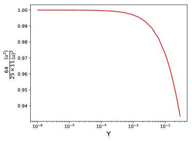
Figure 1: Mean square photon energy normalized by the square of the mean energy according to (10), for a constant bending radius $\rho$. The vertical scale is normalized such that the approximate relation (9) corresponds to a value of 1.

The classical formulae for synchrotron radiation would also be modified for an interaction length ($\approx\sigma_{x}^{\ast}/\theta_{c}$) shorter than the classical formation length $\rho/\gamma$ Telnov (2018); R. Coisson (1979), with $\rho$ the local bending radius. This “short-magnet” regime is characterized by an “undulator parameter” $K_{\rm max}\equiv 2r_{e}N_{b}/(\sigma_{x}\theta_{c})<1$, while the classical radiation spectrum applies for $K_{\rm max}>1$. As we will see below, for all the cases of interest $K_{\rm max}\geq 3$, so that the effect of short-magnet radiation can be neglected.

In the case of a real bunch collision, the relation between $<u>$ and $<u^{2}>$ is further modified, however, for another reason: The local bending radius is not constant, but varies with the transverse and longitudinal position of the colliding particle, and with the time during the collision K. Oide (2017); M.A. Valdivia Garcia and D. El Khechen, K. Oide, and F. Zimmermann (2018). Indeed, while at constant bending radius $\rho$ we have Sands (1969) $\langle u\rangle=4/(5\sqrt{3})\hbar c\gamma^{3}/\rho$, and $<u^{2}>$ well represented by (9), in general (9) must be modified as

$$\langle u^{2}\rangle\approx Z_{\rm c}\frac{25\times 11}{64}\langle u\rangle^{2}\;$$ (11)

where the correction factor $Z_{\rm c}$ is related to the variation of $1/\rho$ in time and space:

$$Z_{\rm c}\equiv\frac{\left\langle 1/\rho^{2}\right\rangle_{x,y,s,t}}{\langle 1/\rho\rangle_{x,y,s,t}^{2}}\;,$$ (12)

where $\langle...\rangle$ denotes the bunch average in space $(x,y,s)$ and time $t$ during a collision.

To treat the case of a nonzero crossing angle, we consider the collision in a co-moving (boosted) frame K. Hirata (1995), where the collision is “head-on”, but both bunches are tilted by an opposite angle of magnitude $\theta_{c}/2$. In first approximation, for the future circular colliders considered, we may ignore the disruption effects K. Yokoya and P. Chen (1992), and we also neglect the rms angular beam divergence compared with the crossing angle $\theta_{c}$. We do take into account the vertical hourglass effect by considering a vertical rms beam size which changes with longitudinal position $s$ as

$$\sigma_{y}(s)=\sqrt{\varepsilon_{y}\left(\beta_{y}^{\ast}+\frac{s^{2}}{\beta_{y}^{\ast}}\right)}\;,$$ (13)

where $\varepsilon_{y}$ denotes the vertical rms emittance and $\beta_{y}^{\ast}$ the vertical beta function at the focal point. Under these assumptions, the inverse local bending radius $\rho$ at transverse coordinates ($x$, $y$), and longitudinal coordinates $s$ (along the beam line) and $z$ (co-moving, along the bunch, with $z=0$ referring to the centre of the bunch, and $z=(s-ct)$; where $t$ is time and $c$ the speed of light) can be approximated as Ziemann (1991)

$$\frac{1}{\rho(x,y,s,z)}=\left|\mathcal{F}\left(x-s\frac{\theta_{c}}{2},y,\sigma_{y}(s)\right)\right|$$ (14)

$$\frac{2N_{b}r_{e}}{\gamma\sigma_{z}}\sqrt{\frac{2}{\pi}}\exp\left(-\frac{2(s-\frac{z}{2})^{2}}{\sigma_{z}^{2}}\right)$$

where $\mathcal{F}(x,y,\sigma_{y}(s))$ may be expressed in terms of the complex error function $w$ as M. Bassetti, G.A. Erskine (1980)

$$\mathcal{F}(x,y,\sigma_{y}(s))=\frac{\sqrt{\pi}}{\sqrt{2}({\sigma_{x}}^{2}-{\sigma_{y}}^{2}(s))}$$ (15)

$$\left(w\left[\frac{x+iy}{\sqrt{2({\sigma_{x}}^{2}-{\sigma_{y}}^{2}(s))}}\right]\right.$$

$$\left.-e^{-\frac{x^{2}}{{2\sigma_{x}}^{2}}-\frac{y^{2}}{{2\sigma_{y}}^{2}(s)}}w\left[\frac{\frac{x\sigma_{y}(s)}{\sigma_{x}}+i\frac{y\sigma_{x}}{\sigma_{y}(s)}}{\sqrt{2({\sigma_{x}}^{2}-{\sigma_{y}}^{2}(s))}}\right]\right)\;.$$

Including the crossing angle and the hourglass effect, the average inverse bending radius is obtained as a quadruple integral of (14) over the four dimensions:

$$\left<\frac{1}{\rho}\right>=\int_{x,y,z,s}dx\;dy\;dz\;ds\;\frac{1}{\rho(x,y,s,z)}$$ (16)

$$\frac{\exp\left(-\frac{\left(x+z\frac{\theta_{c}}{2}\right)^{2}}{2\sigma_{x}^{2}}-\frac{y^{2}}{2\sigma_{y}^{2}(s)}-\frac{z^{2}}{2\sigma_{z}^{2}}-\frac{2\left(s-\frac{z}{2}\right)^{2}}{\sigma_{z}^{2}}\right)}{2\pi^{2}\sigma_{x}\sigma_{y}(s)\sigma_{z}^{2}}\;,$$

which can be evaluated numerically. Similarly, we write

$$\left<\frac{1}{\rho^{2}}\right>=\int_{x,y,z,s}dx\;dy\;dz\;ds\;\frac{1}{\rho(x,y,s,z)^{2}}$$ (17)

$$\frac{\exp\left(-\frac{\left(x+z\frac{\theta_{c}}{2}\right)^{2}}{2\sigma_{x}^{2}}-\frac{y^{2}}{2\sigma_{y}(s)^{2}}-\frac{z^{2}}{2\sigma_{z}^{2}}-\frac{2\left(s-\frac{z}{2}\right)^{2}}{\sigma_{z}^{2}}\right)}{2\pi^{2}\sigma_{x}\sigma_{y}(s)\sigma_{z}^{2}}\;.$$

Using Eqs. (16), and (17) we compute the correction factor $Z_{\rm c}$, which is illustrated in Fig. 2 as a function of the transverse beam-size aspect ratio at the collision point, for different values of crossing angle, holding the beta function $\beta_{y}^{\ast}$ mm, the vertical rms beam size $\sigma_{y}^{\ast}$, and the bunch length $\sigma_{z}$ constant.

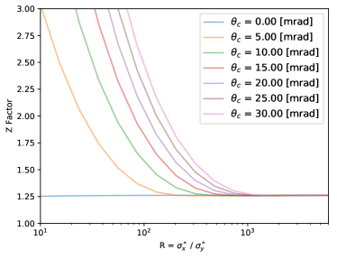
Figure 2: Correction factor $Z_{\rm c}$ versus $R=\sigma_{x}^{\ast}/\sigma_{y}^{\ast}$, for different values of the full crossing angle (colors), with $\beta_{y}^{\ast}=1$ mm, $\sigma_{y}^{\ast}=32$ nm, and $\sigma_{z}=1.64$ mm held constant.

Putting everything together, the quantum excitation Sands (1969) from beamstrahlung emitted in a single collision can be written

$$\{n_{\gamma}\left\langle u^{2}\right\rangle\}_{\rm BS}\approx\frac{25\times 11}{36\pi^{3/2}}Z_{c}\frac{r_{e}^{5}N_{b}^{3}\gamma^{2}}{\alpha\sigma_{z}^{2}{\sigma_{x}^{\ast}}^{3}}\frac{1}{\sqrt{1+\Phi_{\rm piw}^{2}}}\;.$$ (18)

Balancing the sum of the excitation due to beamstrahlung and due to arc synchrotron radiation against the radiation damping from the arcs alone (the average energy loss and, hence, the damping effect due to beamstrahlung is negligible Valdivia Garcia and Zimmermann (2016)) yields the total equilibrium emittance $\varepsilon_{x,{\rm tot}}$

$$\varepsilon_{x,{\rm tot}}=\varepsilon_{x,{\rm SR}}+\frac{n_{\rm IP}\tau_{x,{\rm SR}}}{4T_{\rm rev}}\left\{n_{\gamma}<u^{2}>\right\}_{\rm BS}\mathcal{H}_{x}^{*}\;,$$ (19)

and relative rms momentum spread $\delta_{\rm tot}$ as

$$\sigma_{\delta,{\rm tot}}^{2}=\sigma_{\delta,{\rm SR}}^{2}+\frac{n_{\mathrm{IP}}\tau_{E,\mathrm{SR}}}{4T_{\rm rev}}\left\{n_{\gamma}<u^{2}>\right\}_{\rm BS}\;,$$ (20)

where $\tau_{x}$ and $\tau_{E}$ denote the usual horizontal and longitudinal radiation damping times Sands (1969), respectively, $T_{\rm rev}$ the revolution period, and $n_{IP}$ the number of interaction points. The terms with subindex ${\rm SR}$ refer to the standard equilibrium parameters without beamstrahlung. The dispersion invariant ${\cal H}_{x}^{\ast}$ is defined as Sands (1969)

$${\cal H}_{x}^{\ast}\equiv\frac{\left(\beta_{x}^{\ast}{D_{x}^{\prime}}^{\ast}+\alpha_{x}^{\ast}D_{x}^{\ast}\right)^{2}+{D_{x}^{\ast}}^{2}}{\beta_{x}^{\ast}}\;,$$ (21)

where $\beta_{x}^{\ast}$, $\alpha_{x}^{\ast}$, $D_{x}^{\ast}$ and ${D_{x}^{\prime}}^{\ast}$ denote optical beta and alpha function (Twiss parameters), the dispersion and slope of the dispersion at the collision point, respectively.

The beamstrahlung parameters ($\Upsilon$, $\delta_{B}$, $<u>$ and $\rho$) strongly depend on the bunch length. The “total” (equilibrium) bunch length is related to the total energy spread via the classical relation Sands (1969)

$$\sigma_{z,{\rm tot}}=\frac{\alpha_{\rm C}C}{2\pi Q_{s}}\sigma_{\delta,{\rm tot}}\;,$$ (22)

where $Q_{s}$ denotes the synchrotron tune, $C$ the circumference, and $\alpha_{\rm C}$ the momentum compaction factor.

In the case of zero IP dispersion, beamstrahlung excites the beam particles only longitudinally, and the total energy spread follows from the self-consistency relation Ohmi and Zimmermann (2014); Valdivia Garcia and Zimmermann (2016)

$$\sigma_{\delta,{\rm tot}}^{2}=\sigma_{\delta,{\rm SR}}^{2}+\frac{V}{\sigma_{\delta,{\rm tot}}^{2}{\beta^{\ast}_{x}}^{3/2}\varepsilon_{x,{\rm tot}}^{3/2}}\;,$$ (23)

where we have introduced the coefficient

$$V\equiv\frac{25\times 11}{4\times 36\pi^{3/2}\alpha}\;Z_{\rm c}\;\frac{n_{\rm IP}\tau_{E,{\rm SR}}}{T_{\rm rev}}\;\frac{r_{e}^{5}N_{b}^{3}\gamma^{2}(2\pi Q_{s})^{2}}{(\alpha_{\rm C}C)^{2}\sqrt{1+\Phi_{\rm piw}^{2}}}\;.$$ (24)

in which the correction factor (12) enters.

Table 1 presents example parameters from the FCC-ee and CEPC designs. The strong impact of beamstrahlung is evident when comparing the rms bunch length and momentum spread due to standard arc synchrotron radiation, $\sigma_{z{\rm SR}}$ and $\sigma_{\delta{\rm SR}}$, and the corresponding values in collision, $\sigma_{z{\rm BS}}$ and $\sigma_{\delta{\rm BS}}$. Beamstrahlung increases the bunch length and momentum spread by a factor ranging from about 2 to 4, depending on the beam energy.

Table 1: Example beam parameters for CEPC Higgs production The CEPC Study Group (2018) and three operation modes of FCC-ee A. Abada, M. Abbrescia, S. S. AbdusSalam, et al. (2019), illustrating the effect beamstrahlung on the rms relative momentum spread, $\sigma_{\delta{\rm BS}}$, and on the rms bunch length, $\sigma_{z{\rm BS}}$, according to Eqs. (22) and (23), for $n_{\rm IP}=2$ identical IPs. The analytically computed values can be compared with the result of beam-beam tracking simulations for FCC-ee, namely the values $\sigma_{\delta{\rm SIM}}$ and $\sigma_{z{\rm SIM}}$) shown underneath A. Abada, M. Abbrescia, S. S. AbdusSalam, et al. (2019). Parameters calculated in this letter are shown in bold. The last two rows indicate the tolerances on spurious IP dispersion for a transverse emittance growth of less than 10%, based on Eqs. (27 ) and (28), respectively. The FCC-ee simulation values (subindex “SIM”) are from D. Shatilov A. Abada, M. Abbrescia, S. S. AbdusSalam, et al. (2019).

Machine	CEPC	FCC	FCC	FCC
Mode	ZH	Z	WW	ZH
beam energy $E_{b}$ [GeV]	120	45.6	80	120
circumference $C$ [km]	100.02	97.76	97.76	97.76
crossing angle $\theta_{c}$ [mrad]	33	30	30	30
bunches/beam $n_{b}$	242	16640	2000	328
bunch population $N_{b}$ [$10^{10}$]	15	17	15	18
hor. emittance $\varepsilon_{x}$ [nm]	1.21	0.27	0.84	0.63
vert. emittance $\varepsilon_{y}$ [pm]	2.40	1.00	1.70	1.30
mom. compaction $\alpha_{\rm C}$ [$10^{-6}$]	11.10	14.80	14.80	7.30
hor. IP beta $\beta_{x}^{\ast}$ [m]	0.36	0.15	0.20	0.30
vert. IP beta $\beta_{y}^{\ast}$ [mm]	1.5	0.8	1.0	1.0
bunch length $\sigma_{z{\rm SR}}$ [mm]	2.72	3.50	3.00	3.14
bunch length $\mathbf{\bm{\sigma}_{z{\rm\bf BS}}}$ [mm]	3.76	12.58	5.76	5.15
bunch length $\sigma_{z{\rm SIM}}$ [mm]	—	12.1	6.0	5.3
mom. spread $\sigma_{\delta{\rm SR}}$ [$\%$]	0.10	0.038	0.066	0.099
mom. spread $\mathbf{\bm{\sigma}_{\delta{\rm\bf BS}}}$ [$\mathbf{\%}$]	0.138	0.139	0.128	0.165
mom. spread $\sigma_{\delta{\rm SIM}}$ [$\%$]	—	0.132	0.131	0.165
Piwinski angle $\mathbf{\Phi_{\bf{\rm piw},BS}}$	2.97	29.7	6.7	5.62
energy loss / turn $U_{\rm 0}$ [GeV]	1.73	0.036	0.34	1.72
rev. frequency $f_{\rm rev}$ [Hz]	3003	3000	3000	3000
RF frequency $f_{\rm RF}$ [MHz]	650	400	400	400
RF voltage $V_{\rm rf}$ [GV]	2.17	0.10	0.75	2.0
synchrotron tune $Q_{s}$	0.065	0.025	0.051	0.036
longit. damp. time $\tau_{E}$ [ms]	23.4	418.3	77.5	23.0
rev. period $T_{rev}$ [ms]	0.33	0.33	0.33	0.33
no. IPs $n_{IP}$	2	2	2	2
$L_{\rm CDR}$ [$10^{35}$ cm-2s-1]	0.30	23.00	2.80	0.85
$\mathbf{\Upsilon_{\rm max}}$ [$\mathbf{10^{-4}}$]	13.5	14.8	13.1	21.2
$\mathbf{\Upsilon_{\rm ave}}$ [$\mathbf{10^{-4}}$]	5.6	6.1	5.5	8.9
undulator parameter $\mathbf{K_{\rm max}}$	6.5	2.6	4.7	6.4
correction factor $\mathbf{Z_{\rm c}}$	1.47	2.46	1.70	1.69
$\mathbf{\Delta{\cal H}_{x}^{\ast}}$ [$\mathbf{\bm{\mu}}$m] ($\mathbf{\Delta\bm{\varepsilon}_{x}<0.1\varepsilon_{x}}$)	28.7	0.15	4.94	4.15
$\mathbf{\Delta{\cal H}_{y}^{\ast}}$ [nm] ($\mathbf{\Delta\bm{\varepsilon}_{y}<0.1\varepsilon_{y}}$)	56.9	0.58	10.01	8.57

In the presence of nonzero IP dispersion, also the transverse emittance increases due to the beamstrahlung. Considering a small spurious horizontal dispersion at the interaction point (IP), and assuming that $|D_{x}^{\ast}|\sigma_{\delta,{\rm tot}}\ll\sqrt{\beta_{x}^{\ast}\varepsilon_{x}}$, $\varepsilon_{x,{\rm tot}}$ is no longer constant, but determined by the additional equation

$$\varepsilon_{x,{\rm tot}}\approx\varepsilon_{x,{\rm SR}}+\frac{2V{\cal H}_{x}^{\ast}}{\sigma_{\delta,{\rm tot}}^{2}{\beta^{\ast}_{x}}^{3/2}\varepsilon_{x,{\rm tot}}^{3/2}}\;,$$ (25)

which needs to be solved self-consistently together with (23). The equivalent equation, for the case of spurious vertical dispersion, applies to the vertical emittance:

$$\varepsilon_{y,{\rm tot}}\approx\varepsilon_{y,{\rm SR}}+\frac{2V{\cal H}_{y}^{\ast}}{\sigma_{\delta,{\rm tot}}^{2}{\beta^{\ast}_{x}}^{3/2}\varepsilon_{x,{\rm tot}}^{3/2}}\;.$$ (26)

The spurious dispersion at the IP should not be so large as to lead to significant emittance blow up $\Delta\epsilon_{x(y)}/\epsilon_{x,(y)}$ From Eqs. (25) and (26) we derive the corresponding tolerances for the IP dispersion, namely

$$|{\cal H}_{x}^{\ast}|<\frac{\sigma_{\delta,{\rm tot}}^{2}{\beta^{\ast}_{x}}^{3/2}\varepsilon_{x,{\rm SR}}^{5/2}}{2V}\left[\frac{\Delta\varepsilon_{x}}{\varepsilon_{x}}\right]$$ (27)

and

$$|{\cal H}_{y}^{\ast}|<\frac{\sigma_{\delta,{\rm tot}}^{2}{\beta^{\ast}_{x}}^{3/2}\varepsilon_{x,{\rm SR}}^{3/2}\varepsilon_{y,{\rm SR}}}{2V}\left[\frac{\Delta\varepsilon_{y}}{\varepsilon_{y}}\right]\;.$$ (28)

The resulting tolerances on the two dispersion invariants, for a maximum blow up of 10% are shown in the last two rows of Table 1.

In conclusion, beamstrahlung greatly affects the equilibrium beam distribution in future circular Higgs (or electroweak) factories, in particular momentum spread and bunch length, which must be taken into account when designing the next generation of lepton colliders, in addition to the constraints reported in Telnov (2013); Ohmi et al. (2017). The beamstrahlung effect also introduces new tolerances on the IP optics parameters.

We thank A. Blondel, D. El Khechen, P. Janot, K. Ohmi, K. Oide, D. Shatilov, V. Telnov, and K. Yokoya for helpful discussions.

References

- Sands (1969) M. Sands, International School of Physics, Enrico Fermi, Course XLVI: Physics with Intersecting Storage Rings Varenna, Italy, June 16-26, 1969, Conf. Proc. C6906161, 257 (1969).
- A. Abada, M. Abbrescia, S. S. AbdusSalam, et al. (2019) A. Abada, M. Abbrescia, S. S. AbdusSalam, et al., Eur. Phys. J. Spec. Top. 228 (2019).
- The CEPC Study Group (2018) The CEPC Study Group, Institute of High Energy Physics, Chinese Academy of Sciences, arXiv 1809.00285 (2018).
- G. Aad et al. (2018) (ATLAS Collaboration, CMS Collaboration) G. Aad et al. (ATLAS Collaboration, CMS Collaboration), Phys. Rev. Lett. 114 (2018).
- Hofmann and Keil (1978) A. Hofmann and E. Keil, CERN-LEP-70/86 (1978).
- Balakin et al. (1979) V. E. Balakin, G. I. Budker, and A. N. Skrinskij, Proceedings, 6th All Union Conference on Charged Particle Accelerators: Dubna, USSR, 11-13 Oct 1978. Vol. 1+2 , 27 (1979).
- Bassetti et al. (1983) M. Bassetti, J. Bosser, R. Coisson, M. Gygi-Hanney, A. Hofmann, and E. Keil, Proceedings of the 1983 Particle Accelerator Conference (PAC 83): Accelerator Engineering and Technology, Santa Fe, New Mexico March 21-23, 1983, IEEE Trans. Nucl. Sci. 30, 2182 (1983).
- R. Blankenbecler and S.D. Drell (1987) R. Blankenbecler and S.D. Drell, Phys. Rev. D36, 277 (1987).
- Bell and Bell (1988) M. Bell and J. Bell, Part. Accel. 22, 301 (1988).
- K. Yokoya (1986) K. Yokoya, Nucl. Instrum. Meth. A251, 1 (1986).
- K. Yokoya and P. Chen (1992) K. Yokoya and P. Chen, Frontiers of Particle Beams: Intensity Limitations: Proceedings of a Topical Course held by the Joint US-CERN School on Particle Accelerators, Hilton Head Island, South Carolina, 7-14 November 1990, Lect. Notes Phys. 400, 415 (1992).
- Telnov (2013) V. I. Telnov, Phys. Rev. Lett. 110, 114801 (2013), arXiv:1203.6563 [physics.acc-ph] .
- Bogomyagkov et al. (2014) A. Bogomyagkov, E. Levichev, and D. Shatilov, Phys. Rev. ST Accel. Beams 17, 041004 (2014), arXiv:1311.1580 [physics.acc-ph] .
- Ohmi et al. (2017) K. Ohmi, N. Kuroo, K. Oide, D. Zhou, and F. Zimmermann, Phys. Rev. Lett. 119, 134801 (2017).
- K. Yokoya (2012) K. Yokoya, KEK Accelerator Seminar, 15 March 2012 (2012).
- Ohmi and Zimmermann (2014) K. Ohmi and F. Zimmermann, Proceedings, 5th International Particle Accelerator Conference (IPAC 2014): Dresden, Germany, June 15-20, 2014, THPRI004 (2014), 10.18429/JACoW-IPAC2014-THPRI004.
- Valdivia Garcia and Zimmermann (2016) M. A. Valdivia Garcia and F. Zimmermann, Proceedings, 7th International Particle Accelerator Conference (IPAC 2016): Busan, Korea, May 8–13, 2016, WEPMW010 (2016), 10.18429/JACoW-IPAC2016-WEPMW010.
- Valdivia Garcia et al. (2016) M. A. Valdivia Garcia, A. Faus-Golfe, and F. Zimmermann, Proceedings, 7th International Particle Accelerator Conference (IPAC 2016): Busan, Korea, May 8-13, 2016, WEPMW009 (2016), 10.18429/JACoW-IPAC2016-WEPMW009.
- A. Renieri (1975) A. Renieri, Frascati Preprint LNF-75/6-R (1975).
- Sokolov and Ternov (1986) A. A. Sokolov and I. M. Ternov, Radiation from Relativistic Electrons, AIP translation series (AIP, New York, NY, 1986) trans. from the Russian.
- M. A. Valdivia Garcia, F. Zimmermann (2017) M. A. Valdivia Garcia, F. Zimmermann, Proc. CERN-BINP Workshop for Young Scientists in e+e- Colliders, CERN-Proceedings-2017-001 , 1 (2017).
- Frank and Valdivia Garcia (2017) Z. Frank and M. A. Valdivia Garcia, Proceedings, 8th International Particle Accelerator Conference (IPAC 2017): Copenhagen, Denmark, May 14-19, 2017, WEPIK015 (2017), 10.18429/JACoW-IPAC2017-WEPIK015.
- Telnov (2018) V. I. Telnov, presentation at IPAC’2018, WEYGBE3 (2018).
- R. Coisson (1979) R. Coisson, Phys. Rev. A20, 524 (1979).
- K. Oide (2017) K. Oide, “private communication,” (2017).
- M.A. Valdivia Garcia and D. El Khechen, K. Oide, and F. Zimmermann (2018) M.A. Valdivia Garcia and D. El Khechen, K. Oide, and F. Zimmermann, Proceedings, 9th International Particle Accelerator Conference (IPAC 2018): Vancouver, 29 April – 4 May 2018, MOPMF068 (2018), 10.18429/JACoW-IPAC2018-MOPMF068.
- K. Hirata (1995) K. Hirata, Phys. Rev. Lett. 74, 2228 (1995).
- Ziemann (1991) V. Ziemann, Proceedings, 1991 IEEE Particle Accelerator Conference (PAC 1991): Accelerator Science and Technology May 6-9, 1991 San Francisco, California, Conf. Proc. C910506, 3249 (1991).
- M. Bassetti, G.A. Erskine (1980) M. Bassetti, G.A. Erskine, CERN-ISR-TH-80-06 (1980).