Intermediate scattering function of an anisotropic Brownian circle swimmer

Abstract

Microswimmers exhibit noisy circular motion due to asymmetric propulsion mechanisms, their chiral body shape, or by hydrodynamic couplings in the vicinity of surfaces. Here, we employ the Brownian circle swimmer model and characterize theoretically the dynamics in terms of the directly measurable intermediate scattering function. We derive the associated Fokker-Planck equation for the conditional probabilities and provide an exact solution in terms of generalizations of the Mathieu functions. Different spatiotemporal regimes are identified reflecting the bare translational diffusion at large wavenumbers, the persistent circular motion at intermediate wavenumbers and an enhanced effective diffusion at small wavenumbers. In particular, the circular motion of the particle manifests itself in characteristic oscillations at a plateau of the intermediate scattering function for wavenumbers probing the radius.

I Introduction

A plethora of active agents ranging from biological microswimmers to artificially synthesized self-propelled particles exhibit peculiar dynamical behavior while moving in aqueous media where Brownian motion plays a pivotal role Romanczuk et al. (2012); Vicsek and Zafeiris (2012); Marchetti et al. (2013); Elgeti et al. (2015); Bechinger et al. (2016). These active particles are intrinsically out of equilibrium and their transport properties are highly sensitive to their body shape, the symmetry of the propulsion mechanism, and also interactions with interfaces, which all have been shown to induce a chiral swimming pattern. Examples of circular motion close to surfaces include sperms Woolley (2003); Riedel et al. (2005); Böhmer et al. (2005); Friedrich and Jülicher (2008), and bacteria Berg and Turner (1990); DiLuzio et al. (2005); Lauga et al. (2006); Hill et al. (2007); Li et al. (2008); Di Leonardo et al. (2011); Utada et al. (2014), whereas a special type of algae, Chlamydomonas reinhardtii, exhibits a helical swimming trajectory due to an asymmetry in its flagella beat Racey and Hallett (1981, 1983); Martinez et al. (2012). As a consequence of an either simple asymmetric shape or two internal motors propelling into different directions, also artificial microswimmers such as asymmetric Janus particles Kümmel et al. (2013); ten Hagen et al. (2014), bimetallic micromotors Fournier-Bidoz et al. (2005); Marine et al. (2013); Takagi et al. (2013), and self-assembled doublets of spherical Janus particles Ebbens et al. (2010) display circular motion. Moreover, particles, that perform chemotaxis along their self-generated gradient, are expected to follow circular trajectories in a strong chemical field Taktikos et al. (2011).

As observed in experiments, a minor imbalance in the swimming motion can lead to a rich dynamical behavior of these active agents on the macroscopic level. Hence, a profound knowledge on different levels of coarse graining is necessary to fully understand the non-equilibrium physics of these circle swimmers. Hydrodynamic models characterizing the motion of a linked-bead swimmer in bulk Dreyfus et al. (2005); Ledesma-Aguilar et al. (2012) and close to walls Dunstan et al. (2012), and also flagellated microswimmers at a surface Lauga et al. (2006); Shum et al. (2010); Hu et al. (2015) including the full hydrodynamic interactions have predicted circular swimming patterns of these active agents using analytic computations and computer simulations.

In addition to these microscopic theories, mesoscopic models ignoring the origin of the swimming motion and neglecting hydrodynamic interactions have been elaborated in terms of effective non-equilibrium Langevin equations van Teeffelen and Löwen (2008); van Teeffelen et al. (2009); Ebbens et al. (2010); Mijalkov and Volpe (2013); Krüger et al. (2016); Jahanshahi et al. (2017). Here, the main quantity of interest constitutes the mean-square displacement van Teeffelen and Löwen (2008); van Teeffelen et al. (2009), which exhibits an intermediate oscillatory behavior as a genuine fingerprint of the circular motion. These transport properties have been also quantified in experiments using particle tracking and compared to analytical predictions Ebbens et al. (2010); Utada et al. (2014); Krüger et al. (2016).

Another experimentally accessible quantity that contains much more general spatiotemporal information on the particle’s dynamics constitutes the intermediate scattering function $F(k,t)$ Berne and Pecora (1976); Dhont (1996), which measures the dynamics at lag time $t$ and length scales $2\pi/k$. Mathematically, it is obtained by a Fourier transform of the probability density of the displamcents and represents the associated characteristic function Gardiner (2009).

Only recently the intermediate scattering function has been computed analytically for simple run-and-tumble particles Martens et al. (2012) and for active Brownian agents Kurzthaler et al. (2016). Whereas it has also been measured for Chlamydomonas reinhardtii by light scattering experiments Racey and Hallett (1981, 1983), and within the recently developed image based framework of differential dynamic microscopy Martinez et al. (2012), only approximations of the intermediate scattering function of circle swimmers valid at rather small length scales have been worked out Racey and Hallett (1983); Martinez et al. (2012).

Here, we derive the Fokker-Planck equation for the conditional probability density of the displacements of a Brownian circle swimmer. These active agents display persistent circular motion, but are also subject to rotational and anisotropic translational diffusion, which entails the rotational-translational coupling. To quantify the dynamics of these particles, we provide an analytical solution of the intermediate scattering function in terms of generalizations of the Mathieu functions. We numerically evaluate the intermediate scattering function for the full range of length scales and identify different spatiotemporal regimes reflecting the bare translational diffusion, the persistent circular motion and also the enhanced effective diffusion of the circle swimmer. Furthermore, we obtain the low-order moments such as the mean-square and mean-quartic displacement upon expansion of the intermediate scattering function in the wavenumber. In particular, we discuss the non-Gaussian parameter and corroborate our results with computer simulations.

II The model

We assume the particle to move in a plane with constant speed $v$ along its instantaneous orientation $\mathbf{u}(t)=[\cos\vartheta(t),\sin\vartheta(t)]^{T}$ parametrized by the polar angle $\vartheta(t)$. To model the circular motion of the active particle, the orientation $\vartheta(t)$ displays an average drift of constant angular velocity $\omega$ and is also subject to orientational Brownian motion characterized by the rotational diffusion coefficient $D_{\text{rot}}$. Furthermore, the motion displays translational diffusion encoded in the diffusion coefficients parallel $D_{\parallel}$ and perpendicular $D_{\perp}$ to the orientation, see Fig. 1. Hence, the Langevin equations in It$\bar{\text{o}}$ form for the position $\mathbf{r}(t)$ and the orientation $\vartheta(t)$ of an anisotropic circle swimmer assume the form van Teeffelen and Löwen (2008):

$$\mathrm{d}\vartheta =\omega\mathrm{d}t+\sqrt{2D_{\text{rot}}}\mathrm{d}\psi,$$ (1)

$$\mathrm{d}\mathbf{r} =v\mathbf{u}\mathrm{d}t+\left[\sqrt{2D_{\parallel}}\mathbf{u}\mathbf{u}^{T}+\sqrt{2D_{\perp}}(\mathbb{I}-\mathbf{u}\mathbf{u}^{T})\right]\mathrm{d}\boldsymbol{\xi}.$$ (2)

Here, the rotational and translational diffusion are modeled in terms of independent Gaussian white noise processes $\psi(t)$ and $\boldsymbol{\xi}(t)$ of zero mean and delta correlated variance $\langle\psi(t)\psi(t^{\prime})\rangle=\delta(t-t^{\prime})$ and $\langle\xi_{i}(t)\xi_{j}(t^{\prime})\rangle=\delta_{ij}\delta(t-t^{\prime})$ for $i,j=1,2$, respectively. Although there is multiplicative noise in the translational motion, it does not induce noise induced drift since the noise only couples to the orientation. As a consequence the equations assume the same form also in the Stratonovich interpretation.

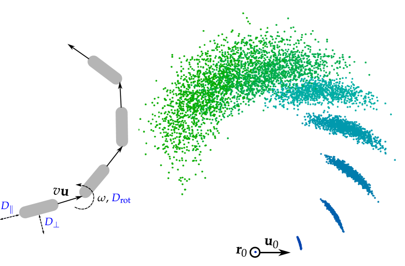
Figure 1: (Left) Model set up and (right) distribution of anisotropic Brownian circle swimmers with the same initial orientation $\mathbf{u}_{0}$, initial position $\mathbf{r}_{0}$, Péclet number $\text{Pe}=\infty$, and quality factor $M=16$. Here, different colors indicate subsequent time steps $t_{i}/\tau_{\text{rot}}\in[0,0.04]$, where $\tau_{\text{rot}}$ denotes the rotational diffusion time.

Typical distributions of circle swimmers, obtained from simulations of the Langevin equations (see Appendix A), reveal a narrow distribution at short times, which displays a circle and thereby broadens due to rotational diffusion at longer times [Fig. 1].

To quantify the deterministic circular motion with respect to the rotational diffusion we introduce the dimensionless quality factor $M$

$$M =\frac{\omega/2\pi}{D_{\text{rot}}}=\frac{\omega}{2\pi}\tau_{\text{rot}},$$ (3)

where $\tau_{\text{rot}}:=1/D_{\text{rot}}$ denotes the rotational diffusion time. Then the angular correlation function of order $n$, $C_{n}(t)=\langle\exp\left[\mathsf{i}n\left(\vartheta(t)-\vartheta(0)\right)\right]\rangle$ fulfills the equation of motion (see Appendix B for a derivation)

$$\frac{\mathrm{d}}{\mathrm{d}t}C_{n}(t)-nD_{\text{rot}}(2\pi\mathsf{i}M-n)C_{n}(t) =0.$$ (4)

The solution

$$C_{n}(t) =\exp(-n^{2}t/\tau_{\text{rot}})\exp(2\pi\mathsf{i}nMt/\tau_{\text{rot}}),$$ (5)

becomes complex, which is a fingerprint of a non-equilibrium process. Here, $\exp(-n^{2}t/\tau_{\text{rot}})$ constitutes the envelope of the oscillations of the real and imaginary part of the angular correlation function (see Fig. 2). In particular, we observe that the quality factor $M$ measures the number of circles a swimmer has completed within the rotational diffusion time $\tau_{\text{rot}}$.

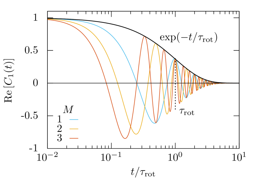
Figure 2: Real part of the angular correlation function $C_{1}(t)$ for different quality factors $M$.

We obtain another dimensionless quantity $\Delta D/\bar{D}$ as ratio between the translational anisotropy $\Delta D=D_{\parallel}-D_{\perp}$ and the mean translational diffusion coefficient $\bar{D}=(D_{\parallel}+D_{\perp})/2$. To illustrate our results we follow Ref. van Teeffelen and Löwen (2008) and use the anisotropy $D_{\parallel}=2D_{\perp}$ inspired by the hydrodynamics for passive rod-like particles in the limit of very large aspect ratio Doi and Edwards (1986). In addition, we also define the Péclet number by $\text{Pe}=av/\bar{D}$, where $a$ denotes the characteristic length $a=\sqrt{3\bar{D}/D_{\text{rot}}}/2$. For a spherical particle in equilibrium $a$ corresponds merely to the radius of the particle. The Péclet number quantifies the relative importance of the persistent swimming motion of the particle with respect to translational diffusion.

The fundamental quantity of interest constitutes the experimentally measurable intermediate scattering function (ISF) Berne and Pecora (1976); Martinez et al. (2012)

$$F(\mathbf{k},t) =\langle\exp[-\mathsf{i}\mathbf{k}\cdot\Delta\mathbf{r}(t)]\rangle.$$ (6)

The ISF can be interpreted as the characteristic function of the random displacement variable $\Delta\mathbf{r}(t)$ and the moments of the stochastic process are obtained as derivatives of the ISF with respect to the wavenumber Gardiner (2009). The ISF of the circle swimmer can be computed by

$$F(\mathbf{k},t) =\int_{0}^{2\pi}\mathrm{d}\vartheta\int_{0}^{2\pi}\frac{\mathrm{d}\vartheta_{0}}{2\pi}\widetilde{\mathbb{P}}(\mathbf{k},\vartheta,t|\vartheta_{0}),$$ (7)

where $\widetilde{\mathbb{P}}(\mathbf{k},\vartheta,t|\vartheta_{0})$ denotes the spatial Fourier transform

$$\widetilde{\mathbb{P}}(\mathbf{k},\vartheta,t|\vartheta_{0}) =\int_{\mathbb{R}^{2}}\mathrm{d}^{2}r\exp(-\mathsf{i}\mathbf{k}\cdot\mathbf{r})\mathbb{P}(\mathbf{r},\vartheta,t|\vartheta_{0}),$$ (8)

of the conditional probability density $\mathbb{P}(\Delta\mathbf{r}=\mathbf{r}-\mathbf{r}_{0},\vartheta,t|\vartheta_{0})$ to find a particle at position $\mathbf{r}$ with orientation $\vartheta$ after a lag time $t$ given that it has been at $\mathbf{r}_{0}$ with orientation $\vartheta_{0}$ at zero lag time, $t=0$.

After averaging over the orientations [Eq. (7)], the motion of the particle is isotropic, and therefore the ISF evaluates to a real function depending on the magnitude of the wavevector $k=|\mathbf{k}|$ only, $F(\mathbf{k},t)=F(k,t)$. In particular, after averaging Eq. (6) over the directions $\varphi=\angle(\mathbf{k},\Delta\mathbf{r}(t))$ of the wavevector $\mathbf{k}$ the ISF reduces to the Bessel function of order zero Arfken and Weber (2005)

$$F(k,t) =\left\langle\int_{0}^{2\pi}\frac{\mathrm{d}\varphi}{2\pi}\exp\left(-\mathsf{i}k|\Delta\mathbf{r}(t)|\cos\varphi\right)\right\rangle$$ (9)

$$=\langle J_{0}(k|\Delta\mathbf{r}(t)|)\rangle.$$ (10)

To obtain an analytic expression for the ISF, we start from Eq. (7) and compute the Fourier transform of the probability density. Therefore we first derive the Fokker-Planck equation for the probability density $\mathbb{P}\equiv\mathbb{P}(\Delta\mathbf{r},\vartheta,t|\vartheta_{0})$, which is an equivalent description of the motion of the circle swimmer as the Langevin equations [Eq. (1)-(2)]. We obtain by standard methods of stochastic calculus Gardiner (2009) the equation of motion

$$\partial_{t}\mathbb{P} =-v\mathbf{u}\cdot\partial_{\mathbf{r}}\mathbb{P}-\omega\partial_{\vartheta}\mathbb{P}+\partial_{\mathbf{r}}\cdot(\mathbf{D}\cdot\partial_{\mathbf{r}}\mathbb{P})+D_{\text{rot}}\partial_{\vartheta}^{2}\mathbb{P},$$ (11)

where $\mathbf{D}$ denotes the translational diffusion tensor $\mathbf{D}=D_{\perp}\mathbb{I}+\Delta D\mathbf{u}\mathbf{u}^{T}$, which couples the translational diffusion to the orientation of the particle. The first two advective terms on the right-hand side of Eq. (11) describe the deterministic active motion and rotational drift of the particle. The remaining terms encode the translational and rotational diffusion, respectively. Then the equation of motion for the corresponding Fourier transform follows

$$\partial_{t}\widetilde{\mathbb{P}} =-\mathsf{i}v\mathbf{u}\cdot\mathbf{k}\widetilde{\mathbb{P}}-\omega\partial_{\vartheta}\widetilde{\mathbb{P}}-[D_{\perp}\mathbf{k}^{2}+\Delta D(\mathbf{u}\cdot\mathbf{k})^{2}]\widetilde{\mathbb{P}}$$

$$\qquad+D_{\text{rot}}\partial^{2}_{\vartheta}\widetilde{\mathbb{P}}.$$ (12)

Counterclockwise swimmers are related to clockwise swimmers by mirror symmetry. In fact, Eq. (12) remains invariant under simultaneous reflections of the wavevector $\mathbf{k}\mapsto\mathbf{k}^{\prime}$ and the orientation $\mathbf{u}\mapsto\mathbf{u}^{\prime}$ across an arbitrarys axis, provided the angular velocity changes sign $\omega\mapsto-\omega$. Choosing as axis of reflection the direction of $\mathbf{k}$ reveals that the ISF is insensitive to the chirality of the particle and does not allow distinguishing whether the agent displays a clockwise or counterclockwise circular swimming motion.

Special cases of the previous equation [Eq. (12)] have already been solved in terms of Mathieu functions for a passive anisotropic Brownian particle ($v=0$ and $\omega=0$) Munk et al. (2009), and also for a three dimensional anisotropic passive Leitmann et al. (2016) and active Brownian particle ($\omega=0$) Kurzthaler et al. (2016). Yet, no solution for the ISF of a Brownian circle swimmer has been elaborated up to now.

We solve Eq. (12) by an expansion of $\widetilde{\mathbb{P}}$ in terms of appropriate eigenfunctions. We choose the direction of the wavevector $\mathbf{k}=k\mathbf{e}_{x}$ such that the equation of motion [Eq. (12)] reduces to

$$\partial_{t}\widetilde{\mathbb{P}} =\bigl{[}-\mathsf{i}vk\cos\vartheta-\omega\partial_{\vartheta}-\left(D_{\perp}+\Delta D\cos^{2}\vartheta\right)k^{2}$$

$$\qquad+D_{\text{rot}}\partial^{2}_{\vartheta}\bigr{]}\widetilde{\mathbb{P}}.$$ (13)

Hence, separation of variables $\exp(-\lambda t)z(\vartheta)$ in terms of angular eigenfunctions $z(\vartheta)$ yields the eigenvalue problem

$$\Bigl{(}\frac{\mathrm{d}^{2}}{\mathrm{d}\vartheta^{2}}-\frac{\mathsf{i}vk}{D_{\text{rot}}}\cos\vartheta-\frac{\Delta Dk^{2}}{D_{\text{rot}}}\cos^{2}\vartheta-2\pi M\frac{\mathrm{d}}{\mathrm{d}\vartheta}$$

$$-\frac{D_{\perp}k^{2}}{D_{\text{rot}}}+\frac{\lambda}{D_{\text{rot}}}\Bigr{)}z(\vartheta)=0,$$ (14)

reminiscent of the Mathieu equation Olver et al. (2010); DLMF . To make connection with the standard form of the Mathieu equation we use a change of variables $x=\vartheta/2$ and obtain an eigenvalue problem $L(q,c,M)z(x)=az(x)$ for the non-hermitian Sturm-Liouville operator

$$L =L(q,c,M)$$

$$=-\frac{\mathrm{d}^{2}}{\mathrm{d}x^{2}}+2q\cos(2x)+c^{2}\cos^{2}(2x)+4\pi M\frac{\mathrm{d}}{\mathrm{d}x},$$ (15)

dependent on the dimensionless parameters $q,c$, and quality factor $M$. Here, we identify the deformation parameters $q=2\mathsf{i}vk/D_{\text{rot}}$ and $c^{2}=4\Delta Dk^{2}/D_{\text{rot}}$ similar to the generalized spheroidal wave functions in Ref. Kurzthaler et al. (2016). In our case, $q$ is purely imaginary, and $c^{2}$ is real but may assume both signs. The separation constant $\lambda$ is connected to the eigenvalue $a$ by $\lambda=D_{\perp}k^{2}+aD_{\text{rot}}/4$.

The eigenfunctions $z(q,c,M,x)$ and the corresponding eigenvalues $a=a(q,c,M)$ are in general complex. Since $q$ is imaginary the Sturm-Liouville operator displays a symmetry: if $z(q,c,M,x)$ is an eigenfunction of $L(q,c,M)$ with eigenvalue $a(q,c,M)$, then $z(q,c,M,x+\pi/2)^{*}$ is eigenfunction to eigenvalue $a(q,c,M)^{*}$. Therefore complex eigenvalues come in complex conjugate pairs. Furthermore, $z(q,c,M,-x)$ is eigenfunction to $L(q,c,-M)$ with eigenvalue $a(q,c,M)$, thus the spectrum does not depend on the chirality of the swimmer.

For the case that $c=M=0$ one recovers the Mathieu equation Olver et al. (2010); DLMF , and by the change of variables we need only the $\pi$-periodic even and odd eigenfunctions $\text{ce}_{2n}(q,x)$ and $\text{se}_{2n+2}(q,x)$. These Mathieu functions are essentially deformed sines and cosines. For $c\neq 0$ but $M=0$ the eigenfunctions remain even and odd functions, and therefore are merely deformations of the Mathieu functions. However, for circle swimmers $M\neq 0$ the operator [Eq. (15)] is no longer invariant under a parity transformation $x\mapsto-x$, and the corresponding eigenfunctions are neither odd nor even in $x$. Therefore, rather than deforming sines and cosines we rely from the very beginning on deformations of the complex exponentials $\exp(2n\mathsf{i}x)$:

$$\text{ee}_{2n}(q,c,M,x) =\sum_{m=-\infty}^{\infty}A_{2m}^{2n}e^{2m\mathsf{i}x},$$ (16)

where $A_{2m}^{2n}$ denotes the $2m-$th Fourier coefficient of $\text{ee}_{2n}(q,c,M,x)$. The eigenfunctions of $L(q,c,M)$ are therefore generalizations of the Mathieu functions $\text{ee}_{2n}(q,c,M,x)$, $n\in\mathbb{Z}$. In Appendix C we show that these eigenfunctions are orthogonal in the sense of

$$\int_{0}^{\pi}\!\mathrm{d}x\ \text{ee}_{2m}(q,c,M,x)\text{ee}_{2n}(q,c,M,-x)=\pi\delta_{mn}.$$ (17)

Thus, the general solution of the Fourier transform $\widetilde{\mathbb{P}}$ is found in terms of an expansion of the corresponding eigenfunctions

$$\widetilde{\mathbb{P}}(\mathbf{k},\vartheta,t|\vartheta_{0})=\frac{e^{-D_{\perp}k^{2}t}}{2\pi}\sum_{n=-\infty}^{\infty}e^{-a_{2n}D_{\text{rot}}t/4}$$

$$\qquad\qquad\times\text{ee}_{2n}(q,c,M,\vartheta/2)\text{ee}_{2n}(q,c,M,-\vartheta_{0}/2).$$ (18)

By completeness of the eigenfunctions, this reproduces indeed the initial condition $\delta(\vartheta-\vartheta_{0}\text{ mod }2\pi)$ for $t=0$. Performing the integrals in Eq. (7), we obtain the analytic expression of the ISF, which constitutes the principal result of this work

$$F(k,t)=\frac{e^{-D_{\perp}k^{2}t}}{4\pi^{2}}\sum_{n=-\infty}^{\infty}e^{-a_{2n}D_{\text{rot}}t/4}$$

$$\qquad\qquad\times\left[\int_{0}^{2\pi}\mathrm{d}\vartheta\ \text{ee}_{2n}(q,c,M,\vartheta/2)\right]^{2}.$$ (19)

Here, the ISF depends explicitely on the diffusion coefficient perpendicular to the particle’s orientation, $D_{\perp}$, the anisotropy is hidden in the parameter $c$, which vanishes for isotropic diffusion. The ISF can then be efficiently evaluated numerically, see Appendix E.

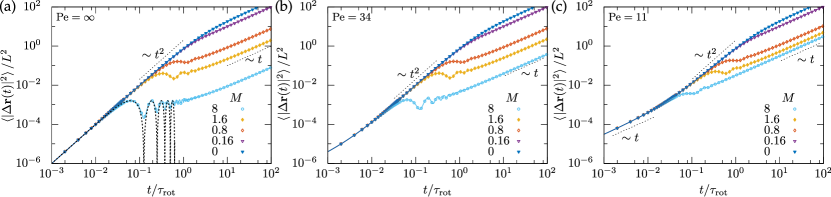
Figure 3: Mean-square displacement $\langle|\Delta\mathbf{r}(t)|^{2}\rangle/L^{2}$ in units of the persistence length $L=v/D_{\text{rot}}$ for an anisotropic ($\Delta D/\bar{D}=2/3$) Brownian circle swimmer for different Péclet numbers $\text{Pe}=av/\bar{D}$ and quality factors $M=\omega\tau_{\text{rot}}/2\pi$ with rotational diffusion time $\tau_{\text{rot}}=1/D_{\text{rot}}$. The black-dashed line in Fig. (a) indicates the mean-square displacement of a deterministic circle swimmer $\langle|\Delta\mathbf{r}(t)|^{2}\rangle=4R^{2}\sin^{2}(\omega t/2)$, where $R=v/\omega$ is the radius of the circular motion. Simulation and theory results are shown with symbols and lines, respectively.

III Exact low-order moments

Most studies consider the low-order moments, such as the mean-square displacement, of active agents only. Since the ISF can be viewed as the moment-generating function of the random displacements, the exact moments can be obtained as a byproduct of our analysis. For consistency we evaluate the mean-square displacement, which has been calculated earlier van Teeffelen and Löwen (2008); Ebbens et al. (2010), and compute for the first time the mean-quartic displacement of an anisotropic Brownian circle swimmer. These are then used as input for the non-Gaussian parameter.

To determine the exact low-order moments of the stochastic process, we expand the ISF [Eq. (10)] up to the fourth order in the wavenumber $k$

$$F(k,t) =1-\frac{k^{2}}{4}\langle|\Delta\mathbf{r}(t)|^{2}\rangle+\frac{k^{4}}{64}\langle|\Delta\mathbf{r}(t)|^{4}\rangle+\mathcal{O}(k^{6}).$$ (20)

Therefore, we apply a time-dependent perturbation theory for small wavenumbers $k$ in the form of a Dyson series Sakurai and Napolitano (2011). For convenience, we rely on the Dirac notation and introduce the scalar product $\langle\varphi|\psi\rangle=(2\pi)^{-1}\int_{0}^{2\pi}\mathrm{d}\vartheta\varphi^{*}(\vartheta)\psi(\vartheta)$. Furthermore, we use the generalized angular basis $\{\mathinner{|{\vartheta}\rangle}\}$, which is orthogonal $\mathinner{\langle{\vartheta|\vartheta_{0}}\rangle}=2\pi\delta(\vartheta-\vartheta_{0})$ and fulfills the closure relation $(2\pi)^{-1}\int_{0}^{2\pi}\mathrm{d}\vartheta|\vartheta\rangle\langle\vartheta|=\mathbb{I}$. Then the isomorphism between angular functions $\psi(\vartheta)$ and states in the Hilbert space becomes manifest $|\psi\rangle\leftrightarrow\psi(\vartheta)=\langle\vartheta|\psi\rangle$. Similarly, we define a time-evolution operator $\widetilde{\mathbb{P}}(\mathbf{k},t)$ via its matrix elements $\widetilde{\mathbb{P}}(\mathbf{k},\vartheta,t|\vartheta_{0})=\langle\vartheta|\widetilde{\mathbb{P}}(\mathbf{k},t)|\vartheta_{0}\rangle/2\pi$, such that $\widetilde{\mathbb{P}}(\mathbf{k},t=0)=\mathbb{I}$. Furthermore, we introduce a generator for the unperturbed time evolution $\hat{H}_{0}$ by $\langle\vartheta|\hat{H}_{0}|\psi\rangle=(\omega\partial_{\vartheta}-D_{\text{rot}}\partial_{\vartheta}^{2})\psi(\vartheta)$ and a perturbation $\hat{V}$ via $\langle\vartheta|\hat{V}|\psi\rangle=\left(\mathsf{i}vk\cos\vartheta+D_{\perp}k^{2}+\Delta Dk^{2}\cos^{2}\vartheta\right)\psi(\vartheta)$. We split the latter into two terms, $\langle\vartheta|\hat{V}_{\text{swim}}|\psi\rangle=\mathsf{i}vk\cos\vartheta\psi(\vartheta)$ and $\langle\vartheta|\hat{V}_{\text{diff}}|\psi\rangle=(D_{\perp}k^{2}+\Delta Dk^{2}\cos^{2}\vartheta)\psi(\vartheta)$, containing perturbations in first and second order in $k$, respectively.

With these definitions we rewrite Eq. (12) in operator form

$$\partial_{t}\widetilde{\mathbb{P}}(\mathbf{k},t) =-\hat{H}_{0}\widetilde{\mathbb{P}}(\mathbf{k},t)-\hat{V}\widetilde{\mathbb{P}}(\mathbf{k},t).$$ (21)

The eigenfunctions of the unperturbed operator $\hat{H}_{0}$ are simply the Fourier modes $|n\rangle$ with angular representation $\mathinner{\langle{\vartheta|n}\rangle}=\exp(\mathsf{i}n\vartheta)$. The corresponding unperturbed eigenvalues read $a_{n}^{0}=D_{\text{rot}}n^{2}+\mathsf{i}n\omega$, in particular, $\hat{H}_{0}\mathinner{|{n}\rangle}=a_{n}^{0}\mathinner{|{n}\rangle}$. The basis fulfills the normalization condition $\mathinner{\langle{m|n}\rangle}=\delta_{mn}$ and closure relation $\sum_{n=-\infty}^{\infty}\mathinner{|{n}\rangle}\mathinner{\langle{n}|}=\mathbb{I}$. The ISF can then be expressed in terms of the eigenbasis of the unperturbed operator by sandwiching the closure relation

$$F (k,t)=\int_{0}^{2\pi}\frac{\mathrm{d}\vartheta}{2\pi}\int_{0}^{2\pi}\frac{\mathrm{d}\vartheta_{0}}{2\pi}\langle\vartheta|\widetilde{\mathbb{P}}(\mathbf{k},t)|\vartheta_{0}\rangle$$

$$=\sum_{m,n=-\infty}^{\infty}\int_{0}^{2\pi}\frac{\mathrm{d}\vartheta}{2\pi}\int_{0}^{2\pi}\frac{\mathrm{d}\vartheta_{0}}{2\pi}\langle\vartheta|m\rangle\langle m|\widetilde{\mathbb{P}}(\mathbf{k},t)|n\rangle\langle n|\vartheta_{0}\rangle$$

$$=\sum_{m,n=-\infty}^{\infty}\int_{0}^{2\pi}\frac{\mathrm{d}\vartheta}{2\pi}e^{\mathsf{i}m\vartheta}\int_{0}^{2\pi}\frac{\mathrm{d}\vartheta_{0}}{2\pi}e^{-\mathsf{i}n\vartheta_{0}}\langle m|\widetilde{\mathbb{P}}(\mathbf{k},t)|n\rangle$$

$$=\langle m=0|\widetilde{\mathbb{P}}(\mathbf{k},t)|n=0\rangle.$$ (22)

To obtain the matrix elements of $\widetilde{\mathbb{P}}(\mathbf{k},t)$, we solve Eq. (21) in terms of a Dyson series Sakurai and Napolitano (2011)

$$\widetilde{\mathbb{P}}(\mathbf{k},t) =e^{-\hat{H}_{0}t}-\int_{0}^{t}\mathrm{d}s\ \ e^{-\hat{H}_{0}(t-s)}\hat{V}e^{-\hat{H}_{0}s}+\mathcal{O}(\hat{V}^{2}).\leavevmode\nobreak\$$ (23)

The initial condition of the time-evolution operator is $\widetilde{\mathbb{P}}(\mathbf{k},t=0)=\mathbbm{1}$, and the unperturbed solution of the propagator is formally expressed by $e^{-\hat{H}_{0}t}$. Hence, the matrix elements of the time-evolution operator up to first order in the perturbation $\hat{V}$ are computed by

$$\langle m|\widetilde{\mathbb{P}}(\mathbf{k},t)|n\rangle =e^{-a_{m}^{0}t}\left[\delta_{mn}-\langle m|\hat{V}|n\rangle\int_{0}^{t}\mathrm{d}s\ e^{-(a_{n}^{0}-a_{m}^{0})s}\right],$$ (24)

with the matrix elements of the perturbation

$$\langle m|\hat{V}|n\rangle =\left(D_{\perp}+\frac{\Delta D}{2}\right)k^{2}\delta_{mn}+\frac{\mathsf{i}vk}{2}\left(\delta_{m,n+1}+\delta_{m,n-1}\right)$$

$$\ \ \ \ +\frac{\Delta Dk^{2}}{4}\left(\delta_{m,n+2}+\delta_{m,n-2}\right).$$ (25)

To obtain an expansion of the ISF up to the fourth order in the wavenumber $\mathcal{O}(k^{4})$ we have to extend the Dyson series up to the order $\mathcal{O}(\hat{V}_{\text{swim}}^{4},\hat{V}_{\text{diff}}^{2},\hat{V}_{\text{swim}}^{2}\hat{V}_{\text{diff}},\hat{V}_{\text{diff}}\hat{V}_{\text{swim}}^{2},\hat{V}_{\text{swim}}\hat{V}_{\text{diff}}\hat{V}_{\text{swim}})$. Then the zeroth matrix element $m=n=0$ of the Fourier transform constitutes the expanded ISF up to $k^{4}$. The computations are rather lengthy but analog to the ones, that have been presented before.

III.1 Mean-square displacement

Evaluating the expansion of the ISF for small wavenumbers [Eq. (22)] and comparing with Eq. (20), we obtain the mean-square displacement of an anisotropic Brownian circle swimmer

$$\langle|\Delta\mathbf{r}(t)|^{2}\rangle =\frac{2e^{-D_{\text{rot}}t}v^{2}}{\left(D_{\text{rot}}^{2}+\omega^{2}\right)^{2}}\Bigl{[}e^{D_{\text{rot}}t}\bigl{(}D_{\text{rot}}^{2}(D_{\text{rot}}t-1)$$

$$\ \ +\omega^{2}(D_{\text{rot}}t+1)\bigr{)}+(D_{\text{rot}}^{2}-\omega^{2})\cos(\omega t)$$

$$\ \ -2D_{\text{rot}}\omega\sin(\omega t)\Bigr{]}+4\bar{D}t,$$ (26)

which has already been computed in Ref. van Teeffelen and Löwen (2008); Ebbens et al. (2010).

The problem displays three characteristic times: the time the particle diffuses translationally before active motion dominates, $\tau_{\text{diff}}:=\bar{D}/v^{2}$, the rotational diffusion time $\tau_{\text{rot}}$ and the time a particle needs to complete a circle, $\tau_{\omega}:=2\pi/\omega$. If $\tau_{\omega},\tau_{\text{rot}}\lesssim\tau_{\text{diff}}$ translational diffusion dominates the dynamics of the active particle for all times. Similarly, if $\tau_{\omega}\gtrsim\tau_{\text{rot}}$, the orientation of the particle becomes randomized before the particle can even complete a circle. Therefore, only the ordering $\tau_{\text{diff}}\lesssim\tau_{\omega}\lesssim\tau_{\text{rot}}$ displays novel physics and we restrict the discussion to this case.

For finite Péclet numbers the mean-square displacement increases linearly with diffusion coefficient $\bar{D}$ at times $t\lesssim\tau_{\text{diff}}$, see Fig. 3 (b) and (c). Then, for intermediate times the mean-square displacement increases quadratically in time $v^{2}t^{2}$ due to the persistent swimming motion. Within the rotational diffusion time $\tau_{\text{rot}}$ a particle without torque $M=0$ covers a typical distance $L=v/D_{\text{rot}}$, denoted by the persistence length.

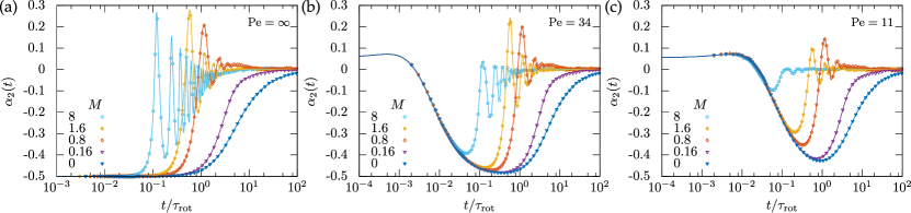
Figure 4: Non-Gaussian parameter $\alpha_{2}(t)$ for an anisotropic Brownian circle swimmer with hydrodynamic anisotropy $\Delta D/\bar{D}=2/3$ for different Péclet numbers $\text{Pe}=av/\bar{D}$ and quality factors $M=\omega\tau_{\text{rot}}/2\pi$ with rotational diffusion time $\tau_{\text{rot}}=1/D_{\text{rot}}$. Simulation and theory results are shown with symbols and lines, respectively.

For Brownian circle swimmers the ballistic increase is followed by oscillations at times $t\gtrsim\tau_{\omega}$, where the particle has completed a circle. In the case of a deterministic swimmer, $D_{\text{rot}}=\bar{D}=0$, the displacement due to the persistent circular motion is thus $|\Delta\mathbf{r}(t)|=2R|\sin(\omega t/2)|$, where $R$ denotes the radius of the circle, $R:=v/\omega$. Then the moments of the displacements evaluate to $\langle|\Delta\mathbf{r}(t)|^{n}\rangle=\left|2R\sin(\omega t/2)\right|^{n}$, which is also indicated in Fig. 3 (a). Hence, the oscillations can be rationalized by the circular motion only, whereas the fading out of the oscillations at longer times is due to the rotational diffusion. In particular, the number of circles $M$ the particle swims during the rotational diffusion time is reflected in the number of oscillations in the mean-square displacement. These oscillations are also smeared out due to translational diffusion for decreasing Péclet numbers at short times [Fig. 3].

For long times the mean-square displacement evolves again linearly in time and we obtain an effective diffusion coefficient $D_{\text{eff}}=\bar{D}+v^{2}D_{\text{rot}}/[2(D_{\text{rot}}^{2}+\omega^{2})]$. In particular, we observe an enhancement of the bare diffusion which is reduced by the torque $D_{\text{eff}}/\bar{D}=1+2\ \text{Pe}^{2}/[3(1+4\pi^{2}M^{2})]$.

III.2 Non-Gaussian parameter

A sensitive indicator that measures the deviation of the stochastic process from a Gaussian process constitutes the non-Gaussian parameter Höfling and Franosch (2013), which is defined in 2D by

$$\alpha_{2}(t) =\frac{1}{2}\frac{\langle|\Delta\mathbf{r}(t)|^{4}\rangle}{\langle|\Delta\mathbf{r}(t)|^{2}\rangle^{2}}-1.$$ (27)

The expression of the mean-quartic displacement is rather lengthy and we refer to Appendix D [Eq. (39)].

For long times $t\gtrsim\tau_{\text{rot}}$ the non-Gaussian parameter tends towards zero for all Péclet numbers and angular velocities, since the motion gets randomized and evolves to an effective diffusion, see Fig. 4.

For infinite Péclet number $\text{Pe}=\infty$ we observe a negative non-Gaussian parameter at short times, $\alpha_{2}(t\rightarrow 0)\rightarrow-1/2$ independent of the angular velocity $\omega$, whereas for finite Péclet number the non-Gaussian parameter approaches a non-negative constant $\alpha_{2}(t\rightarrow 0)\rightarrow\Delta D^{2}/8\bar{D}^{2}$. Note, that the non-Gaussian parameter vanishes for isotropic particles at short times ($\Delta D=0$).

In the case of a deterministic circle swimmer, $D_{\text{rot}}=\bar{D}=0$, we find that the non-Gaussian parameter evaluates to a constant $\alpha_{2}(t)=-1/2$ for all times. This value is indeed observed in the full solution for $\text{Pe}=\infty$ and times $t\lesssim\tau_{\text{rot}}$ where the rotational diffusion has not yet set in (see Fig. 4 (a)).

At intermediate times the non-Gaussian parameter for finite quality factors $M$ approaches the non-Gaussian parameter of an active Brownian particle with $M=0$ reflecting the active swimming motion. This regime is followed by an oscillatory behavior that can be rationalized by the interplay of deterministic circular motion and rotational diffusion of the particle. In particular, similar to the mean-square displacement [Fig. 3] the number $M$ of oscillations for $t\lesssim\tau_{\text{rot}}$ reflects the number of fulfilled circles within the rotational diffusion time. However, these oscillations smear out for finite Péclet number at short times, due to the translational diffusion.

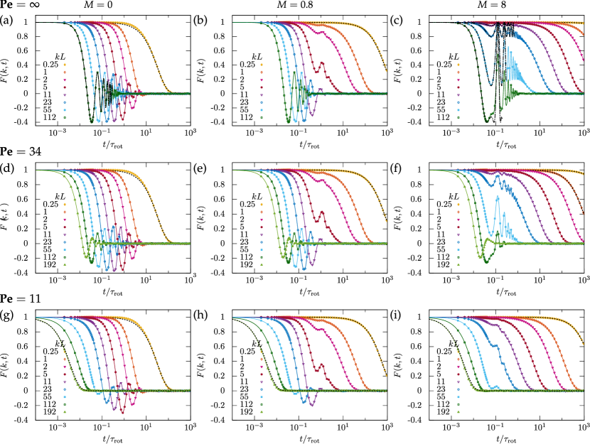
Figure 5: Intermediate scattering function $F(k,t)$ for a single, anisotropic circle swimmer with hydrodynamic anisotropy $\Delta D/\bar{D}=2/3$ for different Péclet numbers $\text{Pe}=av/\bar{D}$ and qualitiy factors $M=\omega\tau_{\text{rot}}/2\pi$. The dashed line represents the effective diffusion $\exp(-D_{\text{eff}}k^{2}t)$ and bare diffusion $\exp(-\bar{D}k^{2}t)$ for large and small wavenumbers, respectively. The dashed-dotted line in Fig. (a) indicates the Bessel function of order zero, $J_{0}(vkt)$, and in Fig. (c) the ISF for persistent circular motion, $J_{0}(2kR|\sin\omega t/2|)$. Simulation and theory results are shown with symbols and lines, respectively.

IV Intermediate scattering function

We have evaluated numerically the intermediate scattering function [Eq. (19)] for arbitrary times and a wide range of length scales measured in terms of the persistence length $kL$, and compare different Péclet numbers Pe and quality factors $M$, see Fig. 5.

For small wavenumbers the ISF can be approximated by an enhanced effective diffusion $\exp(-D_{\text{eff}}k^{2}t)$, where the diffusion coefficient $D_{\text{eff}}$ is taken from the slope of the mean-square displacement at long times [Eq. (26)]. In particular, a reduction of the effective diffusion is observed with increasing quality factor $M$ [Fig. 5].

For large wavenumbers and Péclet number $\text{Pe}=11$ [Fig. 5  (g)-(i)] the intermediate scattering function again approaches an exponential $\exp(-\bar{D}k^{2}t)$ reflecting the bare translational diffusion. A similar behavior occurs for $\text{Pe}=34$ at even higher wavenumbers (not shown).

In contrast, for infinite Péclet number $\text{Pe}=\infty$ [Fig. 5 (a)-(c)] and vanishing quality factor $M=0$ the trajectories can be approximated by a pure persistent motion $|\Delta\mathbf{r}(t)|=vt$, in particular, the ISF then assumes the form $F(k,t)=J_{0}(vkt)$, as indicated by the dashed-dotted line in Fig. 5 (a). Note that the approximation is only illustrated for $t/\tau_{\text{rot}}\lesssim 0.3$, as for longer times rotational diffusion washes out the oscillations of the Bessel function.

The circular motion of the particle ($M\neq 0$) first becomes apparent in the ISF at times $t\sim\tau_{\omega}$ [Fig. 5 (b),(c),(e),(f),(h),(i)], where the particle completes a full circle of radius $R$ due to the deterministic torque. In particular, the chiral swimming pattern manifests itself in characteristic oscillations at a plateau for wavenumbers $kR\lesssim 2\pi$ (i.e. $kL\lesssim 4\pi^{2}M$) and times $t\sim\tau_{\omega}$, which smear out due to rotational diffusion at longer times, $t\gtrsim\tau_{\text{rot}}$. For the case that $\tau_{\omega}\lesssim\tau_{\text{rot}}$ (i.e. $M\gtrsim 1$) these oscillations can be rationalized using the approximation of the pure persistent circular motion with corresponding ISF, $F(k,t)=J_{0}(2kR|\sin\omega t/2|)$. In particular, in this approximation the ISF displays oscillations between unity and the plateau $J_{0}(2kR)=J_{0}(kL/\pi M)$. These oscillations persist for arbitrarily small wavenumbers, yet, the amplitude $1-J_{0}(kL/\pi M)\approx(kL/2\pi M)^{2}$ becomes small. At infinite Péclet number, the approximation reproduces the ISF for wavenumbers probing the radius of the circular motion and for times $t\lesssim\tau_{\text{rot}}$ (see Fig. 5 (c) black dashed-dotted line). The oscillations at a plateau are also predicted by our analytic theory for small wavenumbers $kL\lesssim 5$ and times $t\sim\tau_{\omega}\lesssim\tau_{\text{rot}}$ and agree with the approximate solution. However, since these oscillations become negligible small, the ISF for small wavenumbers can be approximated by a simple exponential with effective diffusion coefficient, $\exp(-D_{\text{eff}}k^{2}t)$.

For increasing quality factors $M$, the radius of the circular motion decreases ($R=v/\omega=v/(2\pi D_{\text{rot}}M)$), and therefore, these characteristic oscillations occur at even larger wavenumbers, which are required to resolve the circular motion. For times $t\ll\tau_{\omega}$ the ISF reduces to the ISF of pure persistent swimming motion, $F(k,t)=J_{0}(vkt)$, since at these time scales the particle has completed only a small fraction of a circle and, therefore, the motion appears as a straight line.

Moreover, for increasing quality factor $M$ oscillations at a plateau become stronger at intermediate times, whereas the effective diffusion of the particle at large length scales is reduced, and therefore shifts the decaying exponentials $\exp(-D_{\text{eff}}k^{2}t)$ to longer and longer times. Furthermore, for decreasing Péclet numbers these oscillations at a plateau at intermediate times and large wavenumbers are less pronounced or even smeared out due to the translational diffusion.

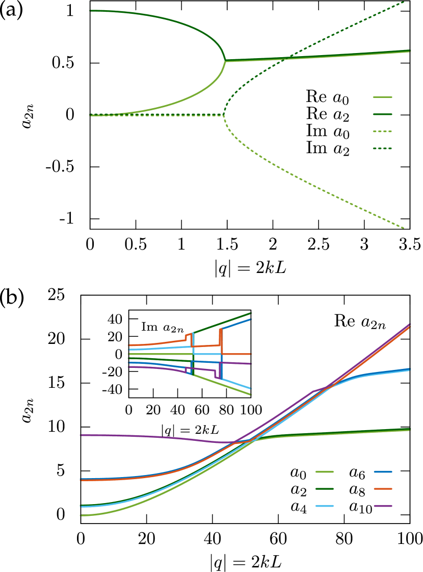
Figure 6: (a) Real (solid line) and imaginary part (dashed line) of the two adjacent eigenvalues $a_{0}$ and $a_{2}$ for Péclet number $\text{Pe}=\infty$ and quality factor $M=0$. (b) Real and imaginary part (inset) of the lowest eigenvalues for Péclet number $\text{Pe}=\infty$ and quality factor $M=0.8$. The eigenvalues depend continuously on the deformation parameter $|q|=2kL=2kv/D_{\text{rot}}$, however, the ordering changes with increasing magnitude.

Interestingly, from a mathematical point of view, these oscillations occur as the operator in Eq. (12) is not Hermitian and therefore allows for pairs of complex conjugated eigenvalues. Here, for $M=0$ and infinite Péclet number $\text{Pe}=\infty$ we find that the two lowest neighboring eigenvalues are real at small wavenumbers, whereas they merge at a certain point $kL=|q|/2=0.75$, where they branch out to a pair of complex conjugates eigenvalues Ziener et al. (2012); Kurzthaler et al. (2016), see Fig. 6 (a). Hence, oscillations in the ISF start to become apparent for wavenumbers larger than $kL>0.75$, whereas at smaller wavenumbers (e.g. $kL=0.25$) the eigenvalues are real, and we observe effective diffusion (compare with Fig. 5 (a)).

Due to the branching points of the eigenvalues, the ISF depends non-analytically on the wavenumber $kL$, and the expansion of the ISF in the wavenumber is anticipated to display a finite radius of convergence. Therefore, the oscillations of the ISF, which become apparent only after the first branching point, cannot be recovered from a perturbation theory in the wavenumber in terms of the low-order moments.

For $M\neq 0$ we find a more intricate behavior of the lowest eigenvalues, which contain complex conjugated pairs for all wavenumbers, in contrast to the case of $M=0$. In particular, the real parts of these eigenvalues merge with that of a lower eigenvalue at small wavenumbers, split up at a certain wavenumber $|q|=2kL$, where they become purely real numbers, and later form a new pair of complex conjugates with the higher adjacent eigenvalue (see Fig. 6 (b)). The eigenvalues depend continuously on $|q|=2kL$, however, they intersect and branch so that the labeling by increasing magnitude changes. Nevertheless, the series expansion of the ISF contains either real eigenvalues or pairs of these complex conjugated eigenvalues such that the solution always remains real.

V Summary and conclusion

We have elaborated an analytic expression for the ISF of an anisotropic Brownian circle swimmer in terms of appropriate eigenfunctions and corroborated our results by stochastic simulations. In addition to oscillations in the ISF reflecting the persistent swimming motion, the chiral swimming pattern of the particle manifests itself in oscillations at a plateau at intermediate times and length scales, where the particle has approximately completed one full circle. These oscillations, either around zero or at a finite plateau, smear out at large wavenumbers due to the bare translational diffusion, and at small wavenumbers due to the rotational diffusion of the particle. In particular, the deterministic torque reduces the effective diffusion of these circle swimmers at large length scales with respect to a straight swimmer.

Furthermore, we have computed exact low-order moments of the stochastic process upon expansion of the ISF in the wavenumber. In particular, we have evaluated the non-Gaussian parameter, which displays oscillations at intermediate times mirroring the interplay of circular swimming motion and rotational diffusion of these active agents. This non-monotonic behavior has also been observed in computer simulations of chiral particles in 3D, subject to isotropic translational diffusion Sevilla (2016). Similar to the non-Gaussian parameter of three dimensional anisotropic particles Kurzthaler et al. (2016), it is positive for short times reflecting the anisotropic diffusion and approaches zero for long times.

Up to now low-order moments such as the mean-square displacement of these circle swimmers have been mainly used to extract relevant motility parameters from experimental observations. In these studies, the long- and short-time diffusivities have been compared to experiments on bimetallic micromotors by Ref. Marine et al. (2013), and the full time dependence of the mean-square displacement has successfully quantified the dynamics of bacteria Utada et al. (2014) and artificial microswimmers Ebbens et al. (2010). However, these low-order moments are to a great extend insensitive to the shape of the probability distribution, whereas more detailed spatiotemporal information on the dynamics of active particles is encoded in the ISF Gardiner (2009). Only recently, the ISF of a dilute suspension of the algae Chlamydomonas reinhardtii has been measured in differential dynamic microscopy (DDM) experiments, and displays characteristic oscillations at a plateau at intermediate times and length scales Martinez et al. (2012) as found within our theory. To determine the transport properties, approximations of the ISF for the motion at small length scales have been used. Here, our analytic theory also predicts the dynamics of these circle swimmers at larger length scales, where rotational diffusion starts to play a pivotal role, and the motion of the particle gets randomized.

The analytic expression for the ISF of a Brownian circle swimmer therefore allows to analyze experimental data of chiral particles for the full range of length scales. For example, it can be used to extract relevant motility parameters of anisotropic Janus particles confined between two glass plates Kümmel et al. (2013); ten Hagen et al. (2014), or to analyze the role of diffusion in the circular motion of bacteria Berg and Turner (1990); DiLuzio et al. (2005); Lauga et al. (2006); Hill et al. (2007); Li et al. (2008); Di Leonardo et al. (2011) or sperms Woolley (2003); Riedel et al. (2005); Böhmer et al. (2005); Friedrich and Jülicher (2008) close to surfaces. Furthermore, the dynamics of a single circle swimmer in a homogeneous environment presents a suitable starting point to analyze their tactic behavior as response to an additional external (e.g. gravitational) force ten Hagen et al. (2014). It also serves as a reference to characterize the non-equilibrium behavior of these chiral particles exposed to spatially heterogeneous media Chepizhko and Peruani (2013); Schirmacher et al. (2015). Similarly, it might be a useful input to establish sorting mechanisms of microswimmers according to their (chiral) transport properties Mijalkov and Volpe (2013); Chen and Ai (2015).

Due to the mirror symmetry of clockwise and anticlockwise circle swimmers, the ISF is insensitive to the chirality, and therefore DDM measurements do not allow detecting the sense of rotation of these active agents. Hence, to elucidate the interesting question about the role of chirality, one might measure in the framework of particle tracking angular correlation functions of different orders. Furthermore, one can compute analytically and measure experimentally the low-order moments of the displacements for a fixed initial orientation in order to test the relative importance of the angular drift with respect to the rotational diffusion.

Moreover, we have also evaluated the ISFs for straight swimmers in two dimensions, which display qualitatively similar behavior as those in three dimensions Kurzthaler et al. (2016), where the oscillations wash out at small and large wavnumbers due to translational and rotational diffusion, respectively. Quantitatively, the amplitudes of the oscillations are predicted to be stronger for particles moving in a plane, which can solely be traced back to the dimension of the system, as the Péclet numbers and the relation of the diffusion coefficients are the same.

We anticipate that the analytic expressions for the ISF of anisotropic particles in three dimensions Kurzthaler et al. (2016), simple run-and-tumble particles Martens et al. (2012), and Brownian circle swimmers together permit to discriminate between different swimming behaviors of active particles, whereas the mean-square displacements are sometimes hardly distinguishable. In particular, we have worked out that the occurrence of characteristic oscillations in the ISF at a plateau constitutes a strong indicator for a chiral swimming pattern of active particles.

Appendix

Appendix A Stochastic simulation

The starting point for the stochastic simulations are the Langevin equations [Eqs. (1)- (2)], which are discretized according to the Euler scheme Gardiner (2009),

$$\vartheta(t+\Delta t) =\vartheta(t)+\sqrt{2D_{\text{rot}}\Delta t}N_{\psi}+\omega\Delta t$$ (28)

$$\mathbf{r}(t+\Delta t) =\mathbf{r}(t)+v\mathbf{u}\Delta t+\left[\sqrt{2D_{\parallel}}\mathbf{u}\mathbf{u}^{T}+\sqrt{2D_{\perp}}(\mathbb{I}-\mathbf{u}\mathbf{u}^{T})\right]\sqrt{\Delta t}\mathbf{N}_{\xi},$$ (29)

where $\Delta t$ denotes the discretized time step. Here, $N_{\psi}$ and $\mathbf{N}_{\xi}$ are independent and normally distributed random variables with zero mean and unit variance. To obtain reliable statistics we set the time step $\Delta t=10^{-3}\tau_{\text{rot}}$ and simulate $10^{5}$ particles.

Appendix B Equation of motion for the angular correlation function $C_{n}(t)$

The equation of motion for the angular correlation function $C_{n}(t)=\langle\exp\left[\mathsf{i}n(\vartheta(t)-\vartheta(0))\right]\rangle\equiv\langle c_{n}(t)\rangle$ can be obtained using It$\bar{\text{o}}$’s Lemma Gardiner (2009),

$$\mathrm{d}c_{n}(t) =\left(\mathsf{i}n\omega-n^{2}D_{\text{rot}}\right)c_{n}(t)\mathrm{d}t+\mathsf{i}nc_{n}(t)\mathrm{d}\psi(t),$$ (30)

where $\psi(t)$ denotes a white noise process. Taking the mean, we find immediately the equation of motion for $C_{n}(t)$

$$\frac{\mathrm{d}}{\mathrm{d}t}C_{n}(t)-nD_{\text{rot}}(2\pi\mathsf{i}M-n)C_{n}(t) =0.$$ (31)

Alternatively, one can derive this equation by multiplying the Fokker-Planck equation Eq. (12) for $\mathbf{k}=0$ with $\exp[\mathsf{i}n(\vartheta-\vartheta_{0})]$, averaging over initial and integrating over final angles, and then integrating by parts.

Appendix C Non-hermitian eigenvalue problem 

To show that the generalized Mathieu functions are orthogonal in the sense of Eq. (17), we first define the scalar product for $\pi$-periodic functions $\varphi(x),\psi(x)$ by

$$\langle\varphi|\psi\rangle=\frac{1}{\pi}\int_{0}^{\pi}\varphi(x)^{*}\psi(x)\mathrm{d}x.$$ (32)

The adjoint operator of the Sturm-Liouville operator in Eq. (15) with respect to this scalar product fulfills

$$L^{+}=L(q,c,M)^{+}=-\frac{\mathrm{d}^{2}}{\mathrm{d}x^{2}}+2q^{*}\cos(2x)+c^{2}\cos^{2}(2x)-4\pi M\frac{\mathrm{d}}{\mathrm{d}x}.$$ (33)

Here, we recall that generally if $r_{m}(q,c,M,x)$ is a right-eigenfunction with eigenvalue $a_{m}(q,c,M)$, $Lr_{m}=a_{m}r_{m}$, and $l_{n}(q,c,M,x)$ a left-eigenfunction with eigenvalue $b_{n}(q,c,M)$, $L^{+}l_{n}=b_{n}^{*}l_{n}$, then one finds

$$\langle l_{m}|Lr_{n}\rangle=a_{n}\langle l_{m}|r_{n}\rangle=\langle L^{+}l_{m}|r_{n}\rangle=b_{m}\langle l_{m}|r_{n}\rangle,$$ (34)

and therefore

$$(a_{n}-b_{m})\langle l_{m}|r_{n}\rangle=0.$$ (35)

Then eigenfunctions corresponding to different eigenvalues are mutually orthogonal. If the eigenvalue is the same, we label the eigenfunctions to eigenvalue $a_{m}$ by $\langle l_{m}|$ and $|r_{m}\rangle$.

A direct calculation shows that

$$[L^{+}(q,c,M)l_{n}(q,c,M,x)]^{*} =a_{n}(q,c,M)l_{n}(q,c,M,x)^{*}$$

$$=\left[-\frac{\mathrm{d}^{2}}{\mathrm{d}x^{2}}+2q\cos(2x)+c^{2}\cos^{2}(2x)-4\pi M\frac{\mathrm{d}}{\mathrm{d}x}\right]l_{n}(q,c,M,x)^{*}.$$ (36)

A change of variables $x\mapsto-x$ then yields

$$L(q,c,M)l_{n}(q,c,M,-x)^{*}=a_{n}(q,c,M)l_{n}(q,c,M,-x)^{*},$$ (37)

and we conclude that up to normalization $l_{n}(q,c,M,x)^{*}\propto r_{n}(q,c,M,-x)$. Hence, we choose $l_{n}(q,c,M,x)^{*}=r_{n}(q,c,M,-x)$ and normalize the set of eigenfunctions by $\langle l_{n}|r_{m}\rangle=\delta_{nm}$, which corresponds to the orthogonality relation in Eq. (17).

Furthermore, due to the equality of the eigenvalues $b_{n}=a_{n}$ we find

$$L^{+}(q^{*},c,-M)l_{n}(q^{*},c,-M,x) =a_{n}(q^{*},c,-M)^{*}l_{n}(q^{*},c,-M,x),$$ (38)

and as $L(q,c,M)=L^{+}(q^{*},c,-M)$, we observe by comparison with Eq. (37) that the eigenvalues fulfill the symmetry relation $a_{n}(q,c,M)=a_{n}(q^{*},c,-M)^{*}$.

In addition, for purely imaginary $q$, similar to the discussion in the main text, $z(q,c,M,x+\pi/2)$ is eigenfunction to $L(-q,c,M)$ with eigenvalue $a(q,c,M)$, and therefore the spectrum does not depend on the sign of the velocity.

Appendix D Mean-quartic displacement 

To compute the mean-quartic displacement, we expand the ISF up to the fourth order in the wavenumber $\mathcal{O}(k^{4})$. Therefore, we consider a Dyson series [Eq. (23)] with perturbations including the order $\mathcal{O}(\hat{V}_{\text{swim}}^{4},\hat{V}_{\text{diff}}^{2},\hat{V}_{\text{swim}}^{2}\hat{V}_{\text{diff}},\hat{V}_{\text{diff}}\hat{V}_{\text{swim}}^{2},\hat{V}_{\text{swim}}\hat{V}_{\text{diff}}\hat{V}_{\text{swim}})$. Using the properties of the matrix elements $\langle m|\hat{V}|n\rangle$ [Eq. (25)], which are non-zero only for $m=n,n\pm 1,n\pm 2$, the expansion of the ISF can be determined by solving for a finite number of multifold time-integrals. Since we only need the zeroth matrix element of the time-evolution operator [Eq.(22)], it suffices to consider the modes $m=0,\pm 1,\pm 2$ only, and we obtain the solution by a linear combination of the five modes: $1$, $\exp(-D_{\text{rot}}t)\sin(\omega t)$, $\exp(-D_{\text{rot}}t)\cos(\omega t)$, $\exp(-4D_{\text{rot}}t)\sin(2\omega t)$, and $\exp(-4D_{\text{rot}}t)\cos(2\omega t)$. The computations are lengthy and have therefore been implemented and evaluated in a computer algebra system Wolfram Research (2016).

Comparing the expansion of the ISF to Eq. (20), we obtain the mean-quartic displacement of the Brownian circle swimmer,

$$\langle|\Delta\mathbf{r}(t)|^{4}\rangle=\frac{e^{-4D_{\text{rot}}t}}{\omega\left(D_{\text{rot}}^{2}+\omega^{2}\right)^{4}\left(36D_{\text{rot}}^{4}+13\omega^{2}D_{\text{rot}}^{2}+\omega^{4}\right)^{2}}\Bigl{\{}2\omega\Bigl{[}\left(v^{2}+2D_{\text{rot}}\Delta D\right)\omega^{2}-\Delta D\omega^{3}-D_{\text{rot}}\left(9D_{\text{rot}}\Delta D-5v^{2}\right)\omega$$

$$-6D_{\text{rot}}^{2}\left(v^{2}-3D_{\text{rot}}\Delta D\right)\Bigr{]}\Bigl{[}18\Delta DD_{\text{rot}}^{3}+\left(9\Delta D\omega-6v^{2}\right)D_{\text{rot}}^{2}+\omega\left(2\Delta D\omega-5v^{2}\right)D_{\text{rot}}+\omega^{2}\left(v^{2}+\Delta D\omega\right)\Bigr{]}\left(D_{\text{rot}}^{2}+\omega^{2}\right)^{4}\cos(2\omega t)$$

$$-4\omega^{2}\left(9\Delta DD_{\text{rot}}^{2}-5v^{2}D_{\text{rot}}+\Delta D\omega^{2}\right)\Bigl{[}6\left(3D_{\text{rot}}\Delta D-v^{2}\right)D_{\text{rot}}^{2}+\left(v^{2}+2D_{\text{rot}}\Delta D\right)\omega^{2}\Bigr{]}\left(D_{\text{rot}}^{2}+\omega^{2}\right)^{4}\sin(2\omega t)$$

$$+2e^{4D_{\text{rot}}t}\omega\left(9D_{\text{rot}}^{2}+\omega^{2}\right)^{2}\Bigl{[}\left(4D_{\text{rot}}t+1\right)\Delta D^{2}\omega^{10}+\Bigl{(}\left(2D_{\text{rot}}t+1\right)\left(2D_{\text{rot}}t+3\right)v^{4}+6D_{\text{rot}}\left(4D_{\text{rot}}t+3\right)\Delta Dv^{2}$$

$$+32D_{\text{rot}}^{3}t\Delta D^{2}\Bigr{)}\omega^{8}+D_{\text{rot}}^{2}\Bigl{(}\left(4D_{\text{rot}}t(10D_{\text{rot}}t+21)+27\right)v^{4}+6D_{\text{rot}}\left(28D_{\text{rot}}t+5\right)D_{\text{rot}}\Delta Dv^{2}+2D_{\text{rot}}^{2}\left(44D_{\text{rot}}t-5\right)\Delta D^{2}\Bigr{)}\omega^{6}$$

$$+D_{\text{rot}}^{4}\Bigl{(}3\left(4D_{\text{rot}}t(11D_{\text{rot}}t+16)-61\right)v^{4}+18D_{\text{rot}}\left(20D_{\text{rot}}t-9\right)\Delta Dv^{2}+4D_{\text{rot}}^{2}\left(28D_{\text{rot}}t-5\right)\Delta D^{2}\Bigr{)}\omega^{4}$$

$$+D_{\text{rot}}^{6}\Bigl{(}\left(4D_{\text{rot}}t(40D_{\text{rot}}t-31)-723\right)v^{4}+6D_{\text{rot}}\left(52D_{\text{rot}}t-57\right)\Delta Dv^{2}+D_{\text{rot}}^{2}\left(68D_{\text{rot}}t-15\right)\Delta D^{2}\Bigr{)}\omega^{2}$$

$$+16\bar{D}^{2}t^{2}\left(D_{\text{rot}}^{2}+\omega^{2}\right)^{4}\left(4D_{\text{rot}}^{2}+\omega^{2}\right)^{2}+4D_{\text{rot}}^{8}\Bigl{(}\left(4D_{\text{rot}}t(4D_{\text{rot}}t-15)+87\right)v^{4}+6D_{\text{rot}}\left(4D_{\text{rot}}t-7\right)\Delta Dv^{2}$$

$$+D_{\text{rot}}^{2}\left(4D_{\text{rot}}t-1\right)\Delta D^{2}\Bigr{)}+16\bar{D}tv^{2}\left(D_{\text{rot}}^{2}+\omega^{2}\right)^{2}\left(4D_{\text{rot}}^{2}+\omega^{2}\right)^{2}\left((D_{\text{rot}}t-1)D_{\text{rot}}^{2}+(D_{\text{rot}}t+1)\omega^{2}\right)\Bigr{]}$$

$$+8e^{3D_{\text{rot}}t}v^{2}\left(4D_{\text{rot}}^{2}+\omega^{2}\right)^{2}\Bigl{[}-\omega\Bigl{(}9\left((6D_{\text{rot}}t+49)v^{2}-24D_{\text{rot}}\Delta D\right)D_{\text{rot}}^{8}-4\left((39D_{\text{rot}}t+259)v^{2}+96D_{\text{rot}}\Delta D\right)\omega^{2}D_{\text{rot}}^{6}$$

$$-2\left((108D_{\text{rot}}t-31)v^{2}+56D_{\text{rot}}\Delta D\right)\omega^{4}D_{\text{rot}}^{4}+4\left((1-D_{\text{rot}}t)v^{2}+16D_{\text{rot}}\Delta D\right)\omega^{6}D_{\text{rot}}^{2}$$

$$+\left((2D_{\text{rot}}t+1)v^{2}+8D_{\text{rot}}\Delta D\right)\omega^{8}-4\bar{D}t(D_{\text{rot}}-\omega)(D_{\text{rot}}+\omega)\left(D_{\text{rot}}^{2}+\omega^{2}\right)^{2}\left(9D_{\text{rot}}^{2}+\omega^{2}\right)^{2}\Bigr{)}\cos(\omega t)$$

$$-\Bigl{(}(8\bar{D}D_{\text{rot}}t-\Delta D)\omega^{10}+D_{\text{rot}}\left(160\bar{D}tD_{\text{rot}}^{2}+11\Delta DD_{\text{rot}}+(12D_{\text{rot}}t+5)v^{2}\right)\omega^{8}+2D_{\text{rot}}^{3}\bigl{(}472\bar{D}tD_{\text{rot}}^{2}+107\Delta DD_{\text{rot}}$$

$$+10(5D_{\text{rot}}t+2)v^{2}\bigr{)}\omega^{6}+2D_{\text{rot}}^{5}\left(720\bar{D}tD_{\text{rot}}^{2}+155\Delta DD_{\text{rot}}+(265-46D_{\text{rot}}t)v^{2}\right)\omega^{4}+3D_{\text{rot}}^{7}\bigl{(}216\bar{D}tD_{\text{rot}}^{2}+9\Delta DD_{\text{rot}}$$

$$-20(3D_{\text{rot}}t+16)v^{2}\bigr{)}\omega^{2}+81D_{\text{rot}}^{9}(v^{2}-D_{\text{rot}}\Delta D)\Bigr{)}\sin(\omega t)\Bigr{]}\Bigr{\}}.$$ (39)

Appendix E Numerical evaluation of the eigenfunctions 

To numerically evaluate the ISF [Eq. (19)], the eigenvalues $a_{2n}$ and the integrals of the eigenfunctions $\text{ee}_{2n}(q,c,M,\vartheta/2)$ are needed. Therefore, we insert the expanded eigenfunction [Eq. (16)] into the eigenvalue problem [Eq. (15)] and obtain the relation for the Fourier coefficients

$$\left(a_{2n}-\alpha_{2m}\right)A_{2m}^{2n}-q\left(A_{2m+2}^{2n}+A_{2m-2}^{2n}\right)-\frac{c^{2}}{4}\left(A_{2m+4}^{2n}+A_{2m-4}^{2n}\right) =0,$$ (40)

with coefficients $\alpha_{m}=8\pi\mathsf{i}Mm+4m^{2}+c^{2}/2$. For $c=M=0$ the relation for the Fourier coefficients is identical to that of the conventional even and odd Mathieu functions except for the zeroth mode Olver et al. (2010); DLMF . To compute numerically the Fourier coefficients and eigenvalues, we solve the eigenvalue problem $\textsf{M}\mathbf{A}^{2n}=a_{2n}\mathbf{A}^{2n}$, where the eigenvector contains the Fourier coefficients of the expansion, $\mathbf{A}^{2n}=\left[\ldots,A^{2n}_{-2},A^{2n}_{0},A^{2n}_{2},\ldots\right]^{T}$, and the matrix $\sf{M}$ is a band matrix with diagonal elements $M_{mm}=\alpha_{2m}$, and off-diagonals $M_{m,m-1}=M_{m,m+1}=q$, and $M_{m,m-2}=M_{m,m+2}=c^{2}/4$.

The orthonormalization of the eigenfunction translates in the matrix representation to $\sum_{j=-\infty}^{\infty}A_{2j}^{2m}A_{2j}^{2n}=\delta_{mn}$. To finally evaluate the ISF, we compute the integrals in Eq. (19), which reduce to the zeroth Fourier coefficient, $\int_{0}^{2\pi}\mathrm{d}\vartheta\ \text{ee}_{2n}(q,c,M,\vartheta/2)=2\pi A_{0}^{2n}$. In practice, the matrix is truncated at an appropriate dimension such that the normalization of the ISF at $t=0$ is fulfilled, $\sum_{n=-\infty}^{\infty}A_{0}^{2n}A_{0}^{2n}=1$, with reasonable accuracy.

References

- Romanczuk et al. (2012) P. Romanczuk, M. Bär, W. Ebeling, B. Lindner, and L. Schimansky-Geier, The European Physical Journal Special Topics 202, 1 (2012).
- Vicsek and Zafeiris (2012) T. Vicsek and A. Zafeiris, Physics Reports 517, 71 (2012).
- Marchetti et al. (2013) M. C. Marchetti, J. F. Joanny, S. Ramaswamy, T. B. Liverpool, J. Prost, M. Rao, and R. A. Simha, Rev. Mod. Phys. 85, 1143 (2013).
- Elgeti et al. (2015) J. Elgeti, R. G. Winkler, and G. Gompper, Reports on Progress in Physics 78, 056601 (2015).
- Bechinger et al. (2016) C. Bechinger, R. Di Leonardo, H. Löwen, C. Reichhardt, G. Volpe, and G. Volpe, Rev. Mod. Phys. 88, 045006 (2016).
- Woolley (2003) D. Woolley, Reproduction 126, 259 (2003).
- Riedel et al. (2005) I. H. Riedel, K. Kruse, and J. Howard, Science 309, 300 (2005).
- Böhmer et al. (2005) M. Böhmer, Q. Van, I. Weyand, V. Hagen, M. Beyermann, M. Matsumoto, M. Hoshi, E. Hildebrand, and U. B. Kaupp, The EMBO journal 24, 2741 (2005).
- Friedrich and Jülicher (2008) B. M. Friedrich and F. Jülicher, New Journal of Physics 10, 123025 (2008).
- Berg and Turner (1990) H. Berg and L. Turner, Biophysical Journal 58, 919 (1990).
- DiLuzio et al. (2005) W. R. DiLuzio, L. Turner, M. Mayer, P. Garstecki, D. B. Weibel, H. C. Berg, and G. M. Whitesides, Nature 435, 1271 (2005).
- Lauga et al. (2006) E. Lauga, W. R. DiLuzio, G. M. Whitesides, and H. A. Stone, Biophysical Journal 90, 400 (2006).
- Hill et al. (2007) J. Hill, O. Kalkanci, J. L. McMurry, and H. Koser, Phys. Rev. Lett. 98, 068101 (2007).
- Li et al. (2008) G. Li, L.-K. Tam, and J. X. Tang, Proceedings of the National Academy of Sciences 105, 18355 (2008).
- Di Leonardo et al. (2011) R. Di Leonardo, D. Dell’Arciprete, L. Angelani, and V. Iebba, Phys. Rev. Lett. 106, 038101 (2011).
- Utada et al. (2014) A. S. Utada, R. R. Bennett, J. C. Fong, M. L. Gibiansky, F. H. Yildiz, R. Golestanian, and G. C. Wong, Nature communications 5, 4913 (2014).
- Racey and Hallett (1981) T. Racey and F. Hallett, in Scattering Techniques Applied to Supramolecular and Nonequilibrium Systems (Springer, 1981) pp. 893–898.
- Racey and Hallett (1983) T. Racey and F. Hallett, Journal of Muscle Research & Cell Motility 4, 321 (1983).
- Martinez et al. (2012) V. Martinez, R. Besseling, O. Croze, J. Tailleur, M. Reufer, J. Schwarz-Linek, L. Wilson, M. Bees, and W. Poon, Biophysical Journal 103, 1637 (2012).
- Kümmel et al. (2013) F. Kümmel, B. ten Hagen, R. Wittkowski, I. Buttinoni, R. Eichhorn, G. Volpe, H. Löwen, and C. Bechinger, Phys. Rev. Lett. 110, 198302 (2013).
- ten Hagen et al. (2014) B. ten Hagen, F. Kümmel, R. Wittkowski, D. Takagi, H. Löwen, and C. Bechinger, Nature Communications 5, 4829 (2014).
- Fournier-Bidoz et al. (2005) S. Fournier-Bidoz, A. C. Arsenault, I. Manners, and G. A. Ozin, Chem. Commun. , 441 (2005).
- Marine et al. (2013) N. A. Marine, P. M. Wheat, J. Ault, and J. D. Posner, Phys. Rev. E 87, 052305 (2013).
- Takagi et al. (2013) D. Takagi, A. B. Braunschweig, J. Zhang, and M. J. Shelley, Phys. Rev. Lett. 110, 038301 (2013).
- Ebbens et al. (2010) S. Ebbens, R. A. L. Jones, A. J. Ryan, R. Golestanian, and J. R. Howse, Phys. Rev. E 82, 015304 (2010).
- Taktikos et al. (2011) J. Taktikos, V. Zaburdaev, and H. Stark, Phys. Rev. E 84, 041924 (2011).
- Dreyfus et al. (2005) R. Dreyfus, J. Baudry, and A. H. Stone, The European Physical Journal B - Condensed Matter and Complex Systems 47, 161 (2005).
- Ledesma-Aguilar et al. (2012) R. Ledesma-Aguilar, H. Löwen, and J. M. Yeomans, The European Physical Journal E 35, 1 (2012).
- Dunstan et al. (2012) J. Dunstan, G. Mino, E. Clement, and R. Soto, Physics of Fluids (1994-present) 24, 011901 (2012).
- Shum et al. (2010) H. Shum, E. A. Gaffney, and D. J. Smith, Proceedings of the Royal Society of London A: Mathematical, Physical and Engineering Sciences 466, 1725 (2010).
- Hu et al. (2015) J. Hu, A. Wysocki, R. G. Winkler, and G. Gompper, Scientific Reports 5, 9586 (2015).
- van Teeffelen and Löwen (2008) S. van Teeffelen and H. Löwen, Phys. Rev. E 78, 020101 (2008).
- van Teeffelen et al. (2009) S. van Teeffelen, U. Zimmermann, and H. Löwen, Soft Matter 5, 4510 (2009).
- Mijalkov and Volpe (2013) M. Mijalkov and G. Volpe, Soft Matter 9, 6376 (2013).
- Krüger et al. (2016) C. Krüger, G. Klös, C. Bahr, and C. C. Maass, Phys. Rev. Lett. 117, 048003 (2016).
- Jahanshahi et al. (2017) S. Jahanshahi, H. Löwen, and B. ten Hagen, Phys. Rev. E 95, 022606 (2017).
- Berne and Pecora (1976) B. J. Berne and R. Pecora, Dynamic Light Scattering (John Wiley and Sons, New York, 1976).
- Dhont (1996) J. Dhont, An Introduction to Dynamics of Colloids, Studies in Interface Science (Elsevier Science, 1996).
- Gardiner (2009) C. Gardiner, Stochastic Methods: A Handbook for the Natural and Social Sciences, Springer Series in Synergetics (Springer Berlin Heidelberg, 2009).
- Martens et al. (2012) K. Martens, L. Angelani, R. Di Leonardo, and L. Bocquet, The European Physical Journal E 35, 1 (2012).
- Kurzthaler et al. (2016) C. Kurzthaler, S. Leitmann, and T. Franosch, Scientific Reports 6, 36702 (2016).
- Doi and Edwards (1986) M. Doi and S. F. Edwards, The Theory of Polymer Dynamics (Oxford Science Publications, 1986).
- Arfken and Weber (2005) G. Arfken and H. Weber, Mathematical Methods For Physicists International Edition (Elsevier Science, 2005).
- Munk et al. (2009) T. Munk, F. Höfling, E. Frey, and T. Franosch, Europhysics Letters 85, 30003 (2009).
- Leitmann et al. (2016) S. Leitmann, F. Höfling, and T. Franosch, Phys. Rev. Lett. 117, 097801 (2016).
- Olver et al. (2010) F. W. J. Olver, D. W. Lozier, R. F. Boisvert, and C. W. Clark, eds., NIST Handbook of Mathematical Functions (Cambridge University Press, New York, NY, 2010) print companion to DLMF .
- (47) DLMF, “NIST Digital Library of Mathematical Functions,” http://dlmf.nist.gov/, Release 1.0.10 of 2015-08-07, online companion to Olver et al. (2010).
- Sakurai and Napolitano (2011) J. Sakurai and J. Napolitano, Modern Quantum Mechanics (Addison-Wesley, 2011).
- Höfling and Franosch (2013) F. Höfling and T. Franosch, Reports on Progress in Physics 76, 046602 (2013).
- Ziener et al. (2012) C. H. Ziener, M. Rückl, T. Kampf, W. R. Bauer, and H. P. Schlemmer, J. Comput. Appl. Math. 236, 4513 (2012).
- Sevilla (2016) F. J. Sevilla, Phys. Rev. E 94, 062120 (2016).
- Chepizhko and Peruani (2013) O. Chepizhko and F. Peruani, Phys. Rev. Lett. 111, 160604 (2013).
- Schirmacher et al. (2015) W. Schirmacher, B. Fuchs, F. Höfling, and T. Franosch, Phys. Rev. Lett. 115, 240602 (2015).
- Chen and Ai (2015) Q. Chen and B.-q. Ai, The Journal of chemical physics 143, 104113 (2015).
- Wolfram Research (2016) I. Wolfram Research, “Mathematica 10.4,” (2016).