Cross-field chaotic transport of electrons
by E $\times$ B electron drift instability in Hall thruster

Abstract

A model calculation is presented to characterize the anomalous cross-field transport of electrons in a Hall thruster geometry. The anomalous nature of the transport is attributed to the chaotic dynamics of the electrons arising from their interaction with fluctuating unstable electrostatic fields of the electron cyclotron drift instability that is endemic in these devices. Electrons gain energy from these background waves leading to a significant increase in their temperature along the perpendicular direction $T_{\perp}/T_{\parallel}\sim 4$ and an enhanced cross-field electron transport along the thruster axial direction. It is shown that the wave-particle interaction induces a mean velocity of the electrons along the axial direction, which is of the same order of magnitude as seen in experimental observations.

Keywords : ExB drift instability, Hall thruster, Chaos

PACS :
52.20.Dq Particle orbits
52.25.Fi Transport properties
52.75.Di Ion and plasma propulsion

I Introduction

Hall thrusters Morozov:a are gridless ion sources that are frequently used as space propulsion devices in geostationary satellites and long range missions such as Earth to Moon missions. They have been the subject of many past studies Lafleur:t ; Adam:j ; BoeufGarrigues ; Marusov:n ; Tsikata ; Smirnov:a ; Janes . A salient feature observed in such studies is the presence of a strong cross-field anomalous electron transport along the axial direction of the thruster. This has been consistently observed both in model numerical simulations Lafleur:t ; Adam:j ; BoeufGarrigues as well as in laboratory experiments Janes ; Tsikata ; Smirnov:a , and a detailed understanding of this anomalous transport process is still lacking. Since the efficiency of the thruster decreases with an increase in the anomalous electron transport Smirnov:a , it is important to gain some understanding of the underlying mechanism driving such a transport.

Our present work is motivated by a desire to throw some light on this process, and we attempt to do so by analyzing the characteristics of this transport and developing a physics model to describe the origin of the transport. Since the ionization efficiency in the thruster chamber is more than 90$\%$, the density of neutral atoms is so low that electron collisions cannot explain the high electron flux observed experimentally. Indeed, the electron transport coefficients are 100 times larger than those given by the collisional transport model AdamBoeuf:jcjp . Since the collisional transport fails to explain the observed cross-field electron transport after the channel exit, other explanations have been proposed in the past. Among them the non-collisional transport due to the interaction of electrons with the electric fields of the numerous electrostatic instabilities that can occur is an attractive candidate. Indeed, 2D (azimuthal and axial) PIC simulations Adam:j show that turbulence alone (without any wall conductivity that could not be modeled in this simulation) is able to drive a high enough electron transport to explain anomalous transport. The dominant instability seen in those simulations was also observed experimentally Tsikata and identified theoretically as the ${\mathbf{E}}\times{\mathbf{B}}$ electron drift instability Cavalier .

The ${\mathbf{E}}\times{\mathbf{B}}$ electron drift instability, also called the electron cyclotron drift instability or beam cyclotron instability Gary:s , is observed in a magnetized plasma under conditions when the ion motion is hardly modified by the magnetic field whereas the electrons experience a strong drift, resulting in a huge velocity difference between electrons and ions. The frequency of this instability is much lower than the electron cyclotron frequency ($\omega\ll\omega_{\mathrm{c}}$). Therefore, the resonance condition with the cyclotron harmonics, $\omega-k_{\parallel}v_{\parallel}=n\omega_{\mathrm{c}}$ is not satisfied. The frequency is of the order of the ion acoustic wave frequency.

The mechanism of the instability is the following. Bernstein waves (whose frequencies are multiples of the electron cyclotron frequency) are Doppler-shifted towards low frequencies by the high electron drift velocity and reach the ion acoustic wave range. The instability occurs when the two modes merge GarySanderson:pj . The magnetic field and the electron drift velocity are the main sources of the ${\mathbf{E}}\times{\mathbf{B}}$ electron drift instability. Plasma density, temperature and magnetic field gradients as well as ion flows can also play a role Mikhailovskii . This instability is observed in many magnetized plasma devices like magnetrons for material processing Abolmasov:s , magnetic filters BoeufClauster , Penning gauges Ellison:c , linear magnetized plasma devices dedicated to study cross-field plasma instabilities Matsukuma:m , Hall thrusters Morozov:a and many fusion devices.

The transport resulting directly from this instability has not been quantified yet and the mechanism of the instability-electron interaction in this case has not been studied. This paper proposes a first investigation into those questions based on a simple model calculation. In particular, we study the electrons dynamics in a slowly time varying ($\omega\ll\omega_{\mathrm{c}}$) potential profile in the presence of a constant axial electric field and a radial magnetic field. The ion dynamics and their effect on electrons are not considered in this model, and in that sense in our model the system is not self-consistent.

The paper is organized as follows. In section II, we briefly describe the Hall thruster mechanism and the model considered for the wave dispersion relation and spectrum. In section III, the numerical scheme used for particle trajectory integration is detailed. In section IV, we study the behavior of an electron interacting with only one Fourier mode fulfilling the instability dispersion relation of the ${\mathbf{E}}\times{\mathbf{B}}$ electron drift instability. In section V, we study the behavior of an electron interacting with three Fourier modes. In section VI, we show that due to the strong wave-particle interactions, the dynamics of each electron becomes chaotic, and in the presence of more than one wave, we find a significant amount of cross-field electron transport along the axial direction.

II Elementary model

In a Hall thruster, plasma is formed between two co-axial dielectric cylinders. Electrons are injected from an emissive cathode placed outside the exhaust plane and, due to the presence of the strong radial magnetic field, these electrons start to gyrate around magnetic lines and become magnetized. The combination of the axial electric field and the radial magnetic field generates a strong ${\mathbf{E}}\times{\mathbf{B}}$ drift motion in the azimuthal direction. This creates closed Hall current loops. The magnetized electrons are trapped in this configuration and stay for a long time within the channel. This results in a decrease of the electron conductivity in the axial direction. Xenon atoms injected through the anode at the end of the channel are ionized by the electrons drifting at a high velocity. Since the ions are not magnetized, they are extracted from the plasma and the axial electric field accelerates them from the ionization region without collision, as sketched in Fig. 1. The electrons injected from an emissive cathode help to generate the plasma and also help to neutralize the ion beam.

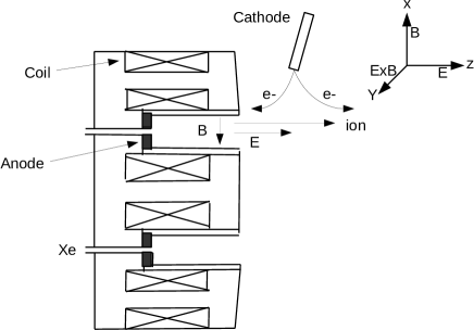
Figure 1: Schematic diagram of Hall thruster. $B$ is the magnetic field, $E_{0}$ is the constant axial electric field, $e^{-}$ denotes electrons, and the top-right sketch presents the Cartesian coordinates for our numerical simulation.

We consider a Cartesian coordinate system for the numerical modeling, with the $x$-direction as the magnetic field direction, the $y$-direction as the ${\mathbf{E}}\times{\mathbf{B}}$ drift direction and the $z$-direction as the constant electric field direction, representing the radial, azimuthal and axial directions respectively of the thruster chamber. Fig. 1 presents these three directions.

In the context of a Hall thruster, using a cold fluid equation for unmagnetized ions and a Vlasov kinetic equation for magnetized electrons, Cavalier et al. Cavalier derived a 3D dispersion relation for the ${\mathbf{E}}\times{\mathbf{B}}$ drift instability in the form

$$1+k^{2}\lambda_{\mathrm{De}}^{2}+g\left(\frac{\omega-k_{y}v_{\mathrm{d}}}{\omega_{\mathrm{ce}}},(k_{x}^{2}+k_{z}^{2})\rho_{\mathrm{e}}^{2},k_{x}^{2}\rho_{\mathrm{e}}^{2}\right)$$

$$-\frac{k^{2}\lambda^{2}_{\mathrm{De}}\omega^{2}_{\mathrm{pi}}}{(\omega-k_{z}v_{\mathrm{i,b}})^{2}} = 0,\qquad$$ (1)

where $\lambda_{\mathrm{De}}$ is the electron Debye length, $v_{\mathrm{d}}=E_{z}/B$ is the electron drift velocity, $v_{\mathrm{i,b}}$ is the ion beam velocity, $\rho_{\mathrm{e}}=v_{\mathrm{the}}/\Omega_{\mathrm{ce}}$ is the electron Larmor radius, $v_{\mathrm{the}}$ is the electron thermal velocity ; $\omega$, $\omega_{\mathrm{ce}}$ and $\omega_{\mathrm{pi}}$ are the mode, electron cyclotron and ion plasma frequency, respectively, while $k_{x}$, $k_{y}$, $k_{z}$ and $k$ are the $x$, $y$ and $z$ components and modulus of wave vector ${\mathbf{k}}$, respectively. $g$ is the Gordeev function Gordeev : $g(\Omega,X,Y)=\frac{\omega}{2Y}\exp(-X)\sum_{m=0}^{\infty}Z(\frac{\Omega-m}{\sqrt{2Y}})I_{m}(X)$ where $Z(x)$ is the plasma dispersion function and $I_{m}$ is the modified Bessel function of first kind. This instability described by Eq. (1) can grow to a sufficient level of turbulence into a non-magnetic ion-acoustic instability with modified angular frequency and growth rate BoeufGarrigues

$$\omega \approx k_{x}v_{\rm{i,b}}+\frac{kc_{\mathrm{s}}}{\sqrt{1+k^{2}\lambda_{\mathrm{De}}^{2}}},$$

$$\gamma \approx \sqrt{\frac{\pi m_{\mathrm{e}}}{8m_{\mathrm{i}}}}\frac{k_{y}v_{\mathrm{d}}}{(1+k^{2}\lambda_{\mathrm{De}}^{2})^{3/2}},$$ (2)

respectively, where $c_{\mathrm{s}}$ is the ion acoustic velocity.

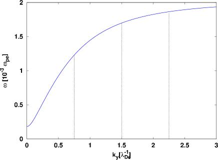
Figure 2: Solutions of the 3D ${\mathbf{E}}\times{\mathbf{B}}$ electron drift instability for $k_{x}=0.03$. The three vertical lines locate the three modes which are taken for our numerical study.

This analytical model for the dispersion relation fits well with experimental data. We consider a constant electric field ${\mathbf{E}}_{0}=E_{0}\,\hat{\mathbf{e}}_{z}$ along the $z$-direction and a constant magnetic field ${\mathbf{B}}=B_{0}\,\hat{\mathbf{e}}_{x}$ along $x$-direction.

Experimentally, the observed propagation angle of the instability-generated wave deviates by $\tan^{-1}({k_{z}/k_{y}})\sim 10-15\,\degree$ from the azimuthal $y$-direction near the thruster exit plane. Further from the exit plane, the propagation becomes progressively more azimuthal Tsikata . Hence, the wave vector along the axial direction $k_{z}\sim 0.2\,k_{y}$, and the electric field along the axial direction is dominated by the stronger constant field $E_{0}\,\hat{\mathbf{e}}_{z}$. Therefore for simplicity, we consider that the unstable modes are confined in $x-y$ (i.e., $r-\theta$) plane only. Then, the time varying part of the potential in $x-y$ plane is constructed as a sum of unstable modes. The total electric field acting on the particle is

$${\mathbf{E}}(x,y,z,t) = \sum_{n}(k_{nx}\hat{\mathbf{e}}_{x}+k_{ny}\hat{\mathbf{e}}_{y})\,{\phi}_{0n}\sin\alpha_{n}(x,y,t)$$ (3)

$$+E_{0}\,\hat{\mathbf{e}}_{z},$$

with local phase $\alpha_{n}(x,y,t)=k_{nx}x+k_{ny}y-\omega_{n}t+\zeta_{n}$, where $n$ is a label for different modes with wave vector ${\mathbf{k}}_{n}$, angular frequency $\omega_{n}$ and phase ${\zeta_{n}}$. ${\mathbf{k}}_{n}$, $\omega_{n}$ follow the dispersion relation eq. (1) and phases $\zeta_{n}$ are random. Here, the position ${\mathbf{r}}$, velocity ${\mathbf{v}}$, time $t$, and potential $\phi_{0}$ are normalized with Debye length $\lambda_{\mathrm{De}}$, thermal velocity $v_{\mathrm{the}}$, reciprocal $\omega_{\mathrm{pe}}^{-1}$ of the electron plasma frequency, and $m_{\mathrm{e}}v_{\mathrm{the}}^{2}/|q_{\mathrm{e}}|$, respectively. We choose the amplitude ${\phi}_{0n}$ of all the modes equal to the saturation potential BoeufGarrigues at the exit plane of the thruster $|\delta\phi_{y,{\mathrm{rms}}}|=T_{\mathrm{e}}/(6\sqrt{2})=0.056\,m_{\mathrm{e}}v_{\mathrm{the}}^{2}$.

We consider three modes $(n=1,2,3)$ with $(k_{nx},k_{ny},\omega_{n})=(0.03,0.75,1.23\times 10^{-3})$, $(0.03,1.5,1.7\times 10^{-3})$ and $(0.03,2.25,1.87\times 10^{-3})$, respectively. The location of these three modes is shown in Fig. 2 by three vertical lines. In normalized units, $|q_{\mathrm{e}}|B_{0}/m_{\mathrm{e}}=0.1\,\omega_{\mathrm{pe}}$, $|q_{\mathrm{e}}|E_{0}/m_{\mathrm{e}}=0.04\,\omega_{\mathrm{pe}}v_{\mathrm{the}}$, and ${v_{\mathrm{d}}=0.4\,v_{\mathrm{the}}}$. Therefore, for all three modes, the $y$-component of phase velocity $\omega_{n}/k_{ny}\ll v_{\mathrm{d}}$.

III Numerical method

The equations of motion of the particle are

$$\frac{{\mathrm{d}}{\mathbf{r}}}{{\mathrm{d}}t}={\mathbf{v}},~{}~{}~{}\frac{{\mathrm{d}}{\mathbf{v}}}{{\mathrm{d}}t}=\frac{q_{\mathrm{e}}}{m_{\mathrm{e}}}({\mathbf{E}}+{\mathbf{v}}\times{\mathbf{B}}).$$ (4)

Because ${\mathbf{E}}$ depends on space, the infinitesimal generators for both equations do not commute, and one uses a time-splitting numerical integration scheme. The first equation is integrated in the form ${\mathbf{r}}(t+\Delta t)={\cal T}_{v,\Delta t}({\mathbf{r}}(t))={\mathbf{r}}(t)+{\mathbf{v}}\Delta t$. For the second equation, we separate the electric integration ${\mathbf{v}}(t+\Delta t)={\cal T}_{E,\Delta t}({\mathbf{v}}(t))={\mathbf{v}}(t)+(q_{\mathrm{e}}/m_{\mathrm{e}}){\mathbf{E}}\Delta t$ from the magnetic integration, which solves only the gyro-motion. For the latter, we use the Boris method boris , formally ${\mathbf{v}}(t+\Delta t)={\cal T}_{B,\Delta t}{\mathbf{v}}(t)$. As a result, we use a second-order symmetric scheme

$$\left(\begin{array}[]{c}{\mathbf{r}}(t+\Delta t)\\ {\mathbf{v}}(t+\Delta t)\end{array}\right)=\mathcal{A}\left(\begin{array}[]{c}{\mathbf{r}}(t)\\ {\mathbf{v}}(t)\end{array}\right),$$ (5)

with the nonlinear map

$$\mathcal{A}={\cal T}_{v,\Delta t/2}\circ{\cal T}_{E,\Delta t/2}\circ{\cal T}_{B,\Delta t}\circ{\cal T}_{E,\Delta t/2}\circ{\cal T}_{v,\Delta t/2}.$$ (6)

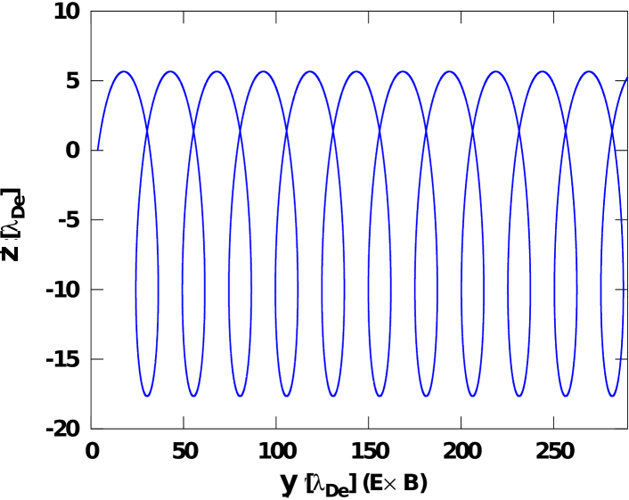
Figure 3: Regular trajectory of a single particle in presence of a constant magnetic field $\omega_{\mathrm{c}}=0.1\,\omega_{\mathrm{pe}}$ and a constant electric field $E_{0}=0.04$.

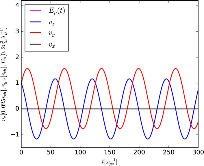
Figure 4: Three components of velocity $v_{x}$ (black), $v_{y}$ (red), $v_{z}$ (blue) and the $y$-component of electric field at the particle location $E_{\mathrm{p}}(t)$ (magenta). Since there is no background electrostatic wave, the electric field amplitude at the particle location vanishes and the magenta line coincides with the black one.

To understand the effect of waves, we first solve the equations of motion Eq. (4) numerically for a single particle trajectory with initial velocity $v_{0x}=0,v_{0y}=1$ and $v_{0z}=1$ in presence of a constant electric field $E_{0}=0.4$ along $z$-direction and a constant magnetic field along $x$-direction such that $\omega_{\mathrm{c}}=0.1\,\omega_{\mathrm{pe}}$. Since there is no background electrostatic wave ($E_{x}=E_{y}=0$), the particle exhibits regular cycloid motion. Therefore, the position co-ordinates $x,y,z$ follow the relation $(y-c-a\tau)^{2}+(z-b)^{2}=c^{2}+b^{2}$, where $a=v_{\mathrm{d}}/\omega_{\mathrm{c}}$, $b=(v_{\mathrm{d}}-v_{0y})/\omega_{\mathrm{c}}$, $c=v_{0z}/\omega_{\mathrm{c}}$ and $\tau=\omega_{\mathrm{c}}t$ and the velocity components are $v_{x}=v_{0x},v_{y}={\rm v_{\perp 0}}\cos(\tau)+v_{\mathrm{d}}$ and $v_{z}={\rm v_{\perp 0}}\sin(\tau)$, where ${\rm v_{\perp 0}}=\sqrt{v_{0z}^{2}+(v_{0y}-v_{\mathrm{d}})^{2}}$ and $(v_{0x},v_{0y},v_{0z})$ are the initial velocity components. Figs 3 and 4 present the trajectory and the velocity components of the particle. Along the $y$-direction, there is a drift velocity $v_{\mathrm{d}}=0.4\,v_{\mathrm{the}}$. Since $v_{x}=0$, the trajectory is confined in the $y-z$ plane.

IV Particle trajectory in presence of one wave

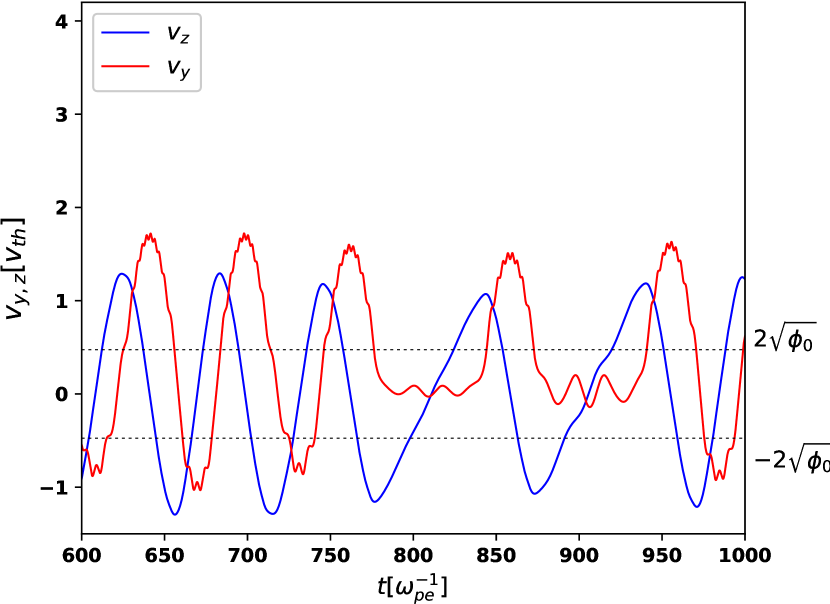
Figure 5: Particle evolution in the presence of a single background electrostatic wave with $n=2$. Velocity components $v_{y}$ (red) and $v_{z}$ (blue) of one particle. Near $t=800$ and $900$, the particle is trapped in the wave potential and it oscillates with the time period $\tau_{\mathrm{b}}=18\,\omega_{\mathrm{pe}}^{-1}$.

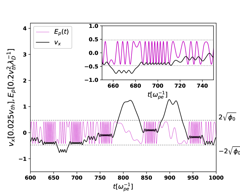
Figure 6: Particle evolution in the presence of a single background electrostatic wave with $n=2$. $v_{x}$ (black solid line), electric field at particle location $E_{\mathrm{p}}(t)$ (magenta line). Black dotted horizontal lines show the location of $\pm 2\sqrt{\phi_{0}}$.

In the presence of a background electrostatic wave, the wave-particle interaction modifies the cyclotron motion. The strength of the wave-particle interaction depends on the wave amplitude and the particle velocity. Fig. 5 presents the time evolution of $v_{y}$ (red line) and $v_{z}$ (blue line), and Fig. 6 presents the time evolution of $v_{x}$ (black line) and the $y$-component $E_{\mathrm{p}}(t)$ of electric field at particle location (magenta line). Due to the cyclotron motion, $v_{y}$ oscillates about the drift velocity $v_{\mathrm{d}}=0.4$. During each cyclotron oscillation, when $|v_{y}|\leq 2\sqrt{\phi_{0}}$ (denoted by black dashed lines) the particle interacts strongly with the electrostatic wave, and the electric field $E_{\mathrm{p}}(t)$ enhances/reduces the $v_{x}$ value by a large amount.

The inset of Fig. 6 presents, during a strong interaction, according to the sign of $E_{\mathrm{p}}$, jumps of $v_{x}$ in positive and negative direction. Moreover, during this strong interaction depending on the local potential profile, the particle may be trapped in the wave potential well and oscillate with the bounce frequency ${\omega_{\mathrm{b}}=0.35\,\omega_{\mathrm{pe}}}$. In Fig. 5 near $t=800$ and $900$, it is trapped. One essential condition for the trapping is ${\omega_{\mathrm{b}}>\omega_{\mathrm{c}}}$, where $\omega_{\mathrm{b}}=k_{y}\sqrt{|q_{\mathrm{e}}|\phi_{0}/m_{\mathrm{e}}}$ is the bounce frequency. Since $k_{y}\gg k_{x}$, the condition for trapping is easily satisfied along the $y$-direction, therefore the particle bounces back and forth along the $y$-direction and moves freely along the $x$-direction. Hence, along the $x$-direction it gains/loses energy from/to the wave, which causes a large change in $v_{x}$. Finally, depending on the local potential value, it may escape from the wave and again start to exhibit cyclotron motion. Therefore, the duration of trapping depends on $v_{x}$ and ${\omega_{\mathrm{b}}/\omega_{\mathrm{c}}}$. It is observed that, for small $v_{x}\ll\sqrt{\phi_{0}}$, this trapping is easily observed for ${\omega_{\mathrm{b}}/\omega_{\mathrm{c}}\geq 2}$.

Outside the strong interaction region, due to the large particle velocity, the electric field at particle location $E_{\mathrm{p}}$ changes rapidly, which generates the small-amplitude fast oscillation in $v_{x}$. The component $v_{y}$ is also modulated due to this fast change in $E_{\mathrm{p}}(t)$. Since the electric field along $z$-direction $E_{0}\,\hat{\mathbf{e}}_{z}$ is constant, the amplitude of the fast oscillation in $v_{z}$ is negligible. The motion along the $z$-direction is coupled with the other two directions due to ${\mathbf{v}}\times{\mathbf{B}}$ term of Lorentz force, therefore $v_{z}$ is also modified during the strong interactions. In Fig. 5 at $t=900$, during trapping, the oscillation of $v_{z}$ is observed with frequency $\omega_{\mathrm{b}}$, on top of cyclotron motion.

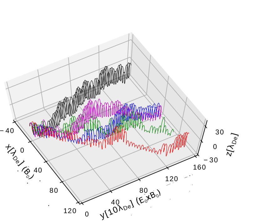
Figure 7: Trajectories of 5 different particles with different initial phase in the presence of a single background electrostatic wave with $n=2$.

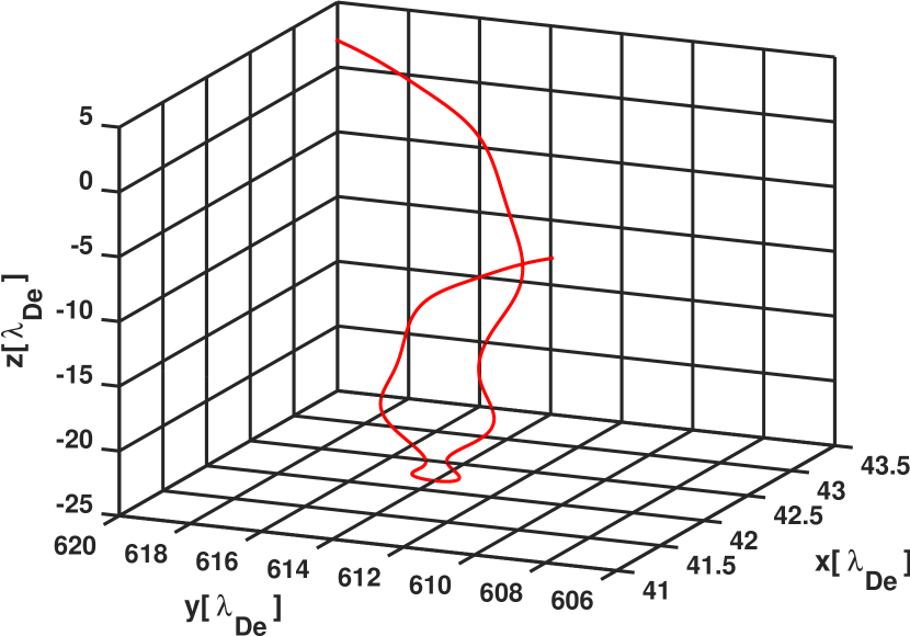
Figure 8: Trajectory of single particle during trapping.

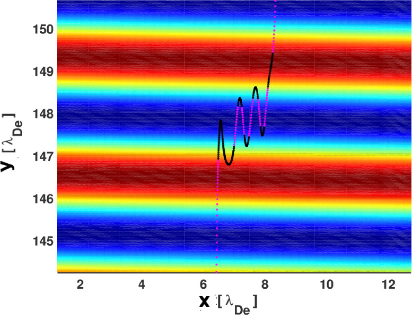
Figure 9: Trapping of particle in the potential well of background wave. Magenta dots: particle energy higher than the maximum potential energy $\phi_{0}$ of the background wave. Black dots: particle energy below $\phi_{0}$. The colour surface plot presents the potential profile of the background wave where red denotes the larger values and blue the lower values.

Fig. 7 displays the trajectories of 5 particles with slightly different initial positions. In the absence of the electrostatic wave, they exhibit cyclotron motion with drifting guiding center, and their trajectories remain confined in the $y-z$ plane. Due to the strong interaction with the electrostatic wave in presence of magnetic field, each trajectory evolves differently and they separate exponentially from each other, so that the dynamics becomes chaotic. Each strong interaction causes a change in the trajectories along $x$, and, depending on the strength of the electric field at particle location, $v_{y}$ may increase or decrease after each strong interaction, which modifies the gyroradius ($r_{\mathrm{b}}=v_{\perp}/\omega_{\mathrm{c}}$) accordingly.

Fig. 8 presents a small portion of trajectory during trapping. Since the particle is trapped along $y$-direction, it oscillates within the wavelength $\lambda=2\pi/k_{y}\sim 4\,\lambda_{\mathrm{De}}$ and Fig. 9 presents the $x-y$ projection of the trajectory during trapping. The colour surface plot presents the background wave potential. Since $\omega\ll\omega_{\mathrm{c}}$, during the strong interaction the wave potential remains constant. The magenta dots mark the particle location when its energy is greater than the maximum potential energy of the electrostatic wave $\phi_{0}$, and black dots are associated with the particle energy below $\phi_{0}$. During climbing up the potential hill, it loses energy and oppositely it gains energy during descent; finally, if, at the top of the potential hill (dark red), the particle energy is greater than the potential energy $\phi_{0}$, it detraps from the potential well. Therefore, the trapping phenomena depend on the wave potential at the particle location : sometimes it may get trapped in the potential well and sometimes it just takes energy from the wave and escapes from the potential well. During trapping, its average $y$ location remains unchanged. Due to this strong wave-particle interaction, the dynamics of the particle becomes chaotic. The duration of strong interaction depends on $\omega_{\mathrm{b}}/\omega_{\mathrm{c}}$, therefore, for a single wave, chaos will occur for amplitudes $\phi_{0}$ satisfying the inequality $\phi_{0}\geq\omega_{\mathrm{c}}^{2}/k_{y}^{2}$. For thruster parameter values, all three waves individually satisfy this criterion.

In the presence of two and three waves, the dynamics becomes more chaotic and this threshold value is reduced. With increase of the potential $\phi_{0}$ and the wave vector $k_{y}$, the bounce frequency of the particle increases, which makes the dynamics more chaotic and particles are trapped more frequently in the electrostatic wave.

V Interactions with three waves: Energy gain and axial transport

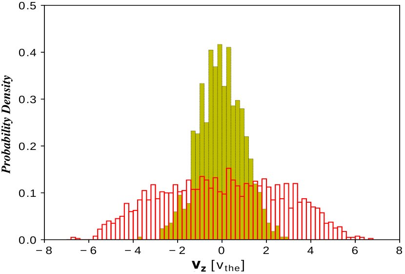
Figure 10: Velocity distribution along $z$ at $t=0$ (yellow solid bar) and at $t=5\times 10^{4}\,\omega_{\mathrm{pe}}^{-1}$ (bar with red boundary).

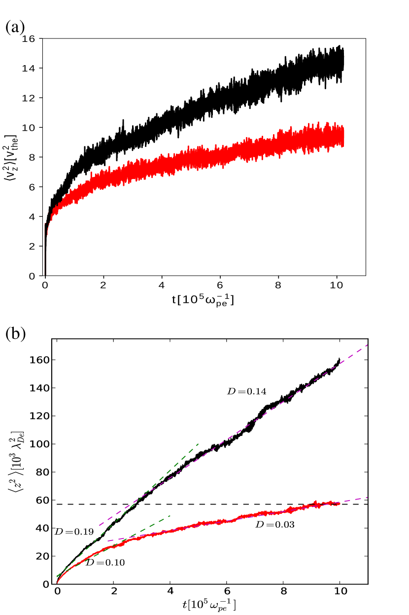
Figure 11: Panels (a) and (b): mean square velocity dispersion $\langle v_{z}^{2}(t)\rangle$ and mean square displacement $\langle z^{2}(t)\rangle$, respectively. The red and black lines correspond to no-boundary and reflecting boundary cases, respectively Panel (b) reveals two diffusion regimes in each curve, namely slopes (0.10, 0.03) for no-boundary and (0.18, 0.14) for reflecting boundary.

To analyze the transport, we consider 1056 particles with random initial positions in the rectangle $0\leq x_{0}\leq 2\pi/k_{1x}$, $0\leq y_{0}\leq 4\pi/k_{1y}$, $z_{0}=0$ and with velocities drawn from a 3D Gaussian distribution with unit standard-deviation (viz. the thermal velocity) along all three directions. Then we evolve their dynamics in the presence of all three waves with equal amplitude $\phi_{n0}={\phi_{0,\mathrm{rms}}}$. For single wave interaction, the Hamiltonian of the dynamics can be written in a time independent form and therefore, though the dynamics remains chaotic, there is no net gain/loss of energy over long time evolution. Hence, due to the chaotic dynamics, in presence of the single wave, we get a very small amount of cross-field transport along the $z$ direction, but the diffusion coefficient is very small.

But in presence of two or more waves, the Hamiltonian is no longer time independent, all the trajectories become chaotic and, due to the wave-particle interaction, they gain energy from the waves. The particles net perpendicular velocity components $v_{y},v_{z}$ increase. After a sufficiently long time-evolution, they form a Gaussian-like velocity distribution profile with higher temperature along $y$- and $z$-directions. Since $E_{x}\ll E_{y,z}$, the increase of the velocity component along the magnetic field is negligible compared to the other two directions. Therefore, the temperature along the magnetic field remains nearly unchanged. Fig. 10 presents the initial ($t=0$) (solid yellow bars) and final $(t=5\times 10^{4}\,\omega_{\mathrm{c}}^{-1})$ (bars with red border) velocity distribution of $v_{z}$, which presents a significant increase of temperature along perpendicular direction $T_{\perp}$ compared to the parallel direction, $T_{\perp}/T_{\parallel}\sim 4$.

In the thruster chamber, there is an insulating boundary along $x$-direction. The width of the annular space in the thruster is $240\,\lambda_{\mathrm{De}}$. Therefore the particles are reflected when they reach the boundary. If there were no reflection, particles would proceed under the same dynamics (red line in Fig. 11(a)-(b)). To account for reflection (black line), we consider the Debye sheath electron potential energy near the wall daren:yu to be ${\phi_{\mathrm{sh}}=20\,{\mathrm{eV}}=0.8\,m_{\mathrm{e}}v_{\mathrm{the}}^{2}}$. Electrons reaching the wall with $v_{x}<\sqrt{0.8}$ are specularly reflected, and electrons with $v_{x}>\sqrt{0.8}$ are isotropically reflected from the wall while conserving their total energy.

Fig. 11(a)-(b) present $\langle v_{z}^{2}(t)\rangle$ and $\langle z^{2}(t)\rangle$ for reflecting boundary (black) and without boundary (red), where $\langle\cdot\rangle$ denotes the average over number of particles for the deviation from the ballistic motion. Thus, $\langle z^{2}\rangle:=\langle(z(t)-v_{z0}t)^{2}\rangle$, $\langle v_{y}\rangle:=\langle(v_{y}(t)-v_{y0})\rangle$, $\langle v_{z}\rangle:=\langle(v_{z}(t)-v_{z0})\rangle$ and $\langle v_{z}^{2}\rangle:=\langle(v_{z}(t)-v_{z0})^{2}\rangle$. The duration of strong interaction with the waves and hence the gain of energy from the waves decrease for larger particle velocity. Therefore, the rate of energy gain in Fig. 11(a) decreases with time for both cases.

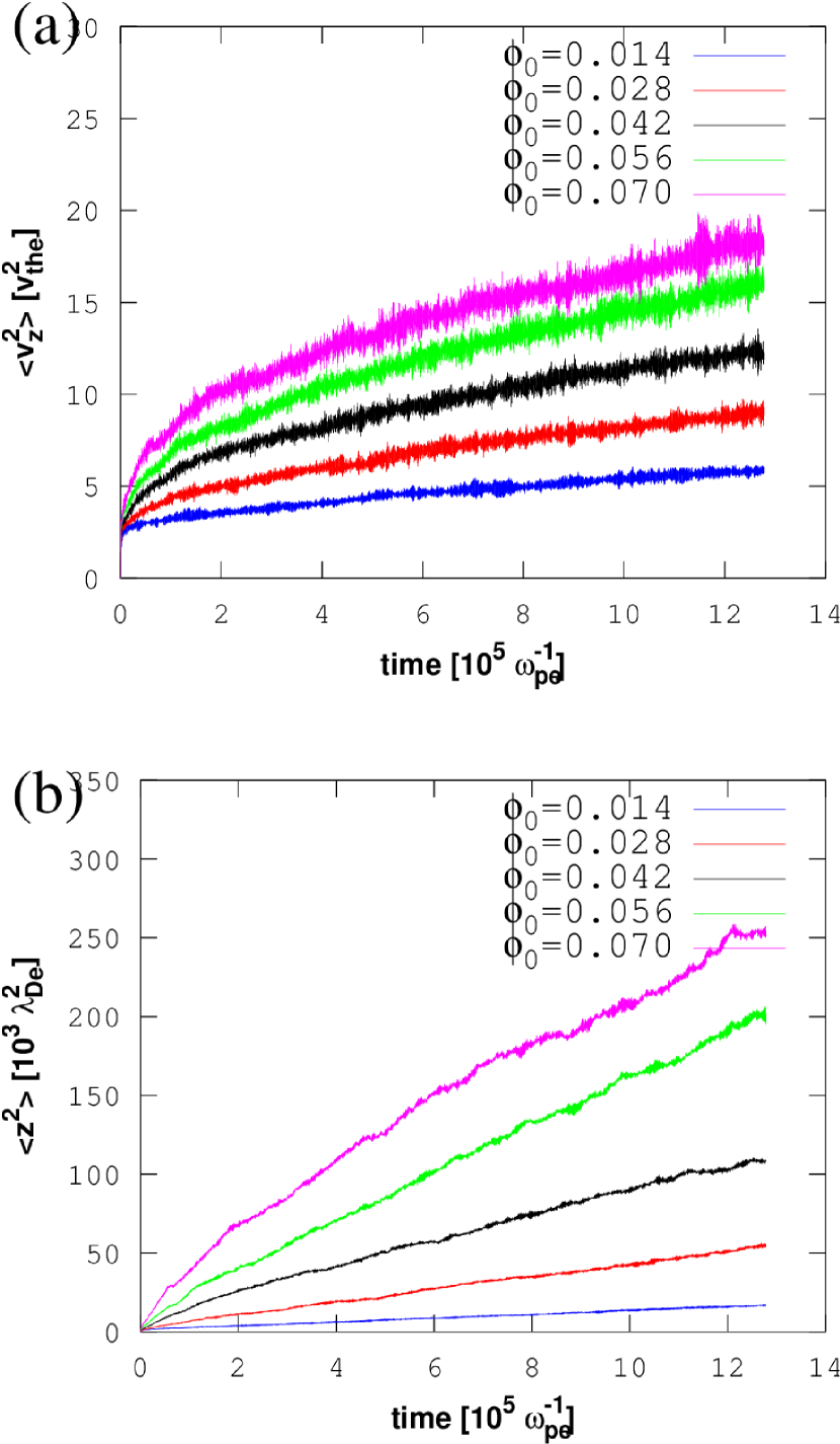
Figure 12: Panel (a): $\langle v_{z}^{2}\rangle$ evolution for different amplitude of the waves. Panel (b): $\langle z^{2}\rangle$ evolution for different wave amplitudes.

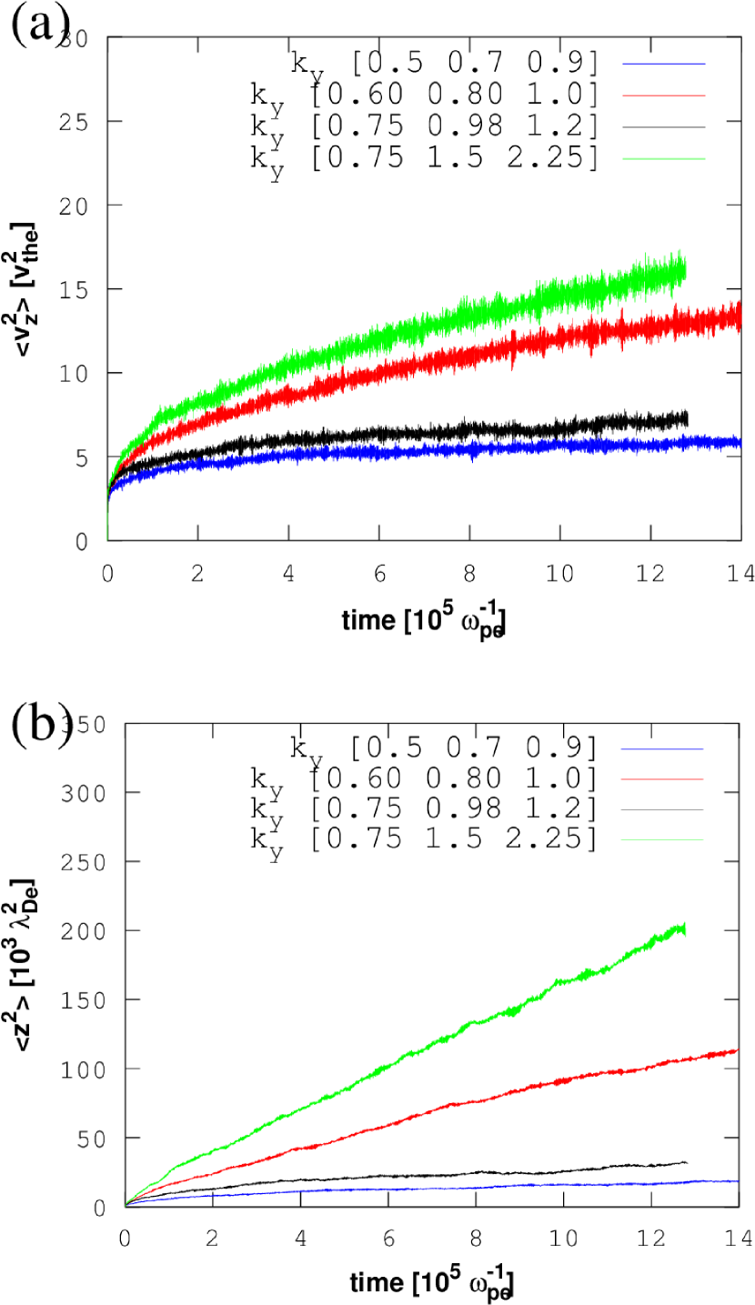
Figure 13: Panel (a): $\langle v_{z}^{2}\rangle$ evolution for different $k_{y}$ values of the waves. Panel (b): $\langle z^{2}\rangle$ evolution for different $k_{y}$ values waves.

In isotropic reflection, the velocity components of the particle are redistributed randomly in three directions, a particle with small $v_{y}$ and $v_{x}$ gains more energy from the electrostatic wave compared to that having higher $v_{y}$ and $v_{x}$. Therefore, in presence of reflecting boundary, particles gain more energy than in absence of reflection. The dashed black line marks the location of thruster outlet along the $z$-direction. Since with reflection they gain more energy, their mean square displacement along $z$-direction crosses the thruster outlet, and they exit from the thruster chamber more quickly than in the case without boundary. For both cases, we found two different regimes of transport. Although the particle motion is not brownian, one may define an effective diffusion coefficient $D={\mathrm{d}}\langle z^{2}\rangle/{\mathrm{d}}t$ in the direction of the static electric field $\bf E_{0}$, as the average of the slope of $\langle z^{2}\rangle$ as a function of time. While the derivative ${\mathrm{d}}\langle z^{2}\rangle/{\mathrm{d}}t$ is fluctuating strongly, the trend is quite stable over time spans on the order of $10^{5}\,\omega_{{\mathrm{pe}}}^{-1}$. Its observed values are $D=(0.1,0.03)$ for no-reflection and $D=(0.18,0.14)$ for reflecting boundary. The change in slope around $t=2\times 10^{5}\,\omega_{\mathrm{pe}}^{-1}$ is related to the different structure formation of the stochastic web, controlling the velocity transport zaslavsky ; leoncini .

The cross-field transport and the energy gain by the particles depend on the duration of wave-particle interaction determined by the ratio $\omega_{\mathrm{b}}/\omega_{\mathrm{c}}$. Since $\omega_{\mathrm{b}}\propto\sqrt{\phi_{0}}$, the cross-field transport and the energy gain from the wave will be higher for higher amplitude of the background waves. Figs 12(a) and (b) present the time evolution of $\langle v_{z}^{2}\rangle$ and $\langle z^{2}\rangle$ for five different amplitudes of the waves $\phi_{0}=0.014,$ $0.028$, $0.042$, $0.056$ and $0.070$.

Moreover, the strength of the electric field and the bounce frequency $\omega_{\mathrm{b}}$ are proportional to the wave number $k_{y}$, therefore $\langle v_{z}^{2}\rangle$ and $\langle z^{2}\rangle$ increase for larger $k_{y}$ of the three waves. Fig. 13(a) and (b) present $\langle v_{z}^{2}\rangle$ and $\langle z^{2}\rangle$ for four different sets of $k_{y}$ values, $(k_{y1},k_{y2},k_{y3})=(0.5,0.7,0.9);(0.6,0.8,1);(0.75,0.98,1.2);(0.75,1.5,2.25)$. For the 2nd and 4th cases, the $k_{y}$ values are the harmonics of $k_{y}=0.2$ and $0.75$, respectively. The large values of $\langle v_{z}^{2}\rangle$ and $\langle z^{2}\rangle$ for these two cases are due to the formation of stochastic webs, which help in long range transport vasilev . For the other two cases where the $k_{y}$ values are not harmonics, there is no stochastic web formation, so that $\langle v_{z}^{2}\rangle$ and $\langle z^{2}\rangle$ are small for those two cases.

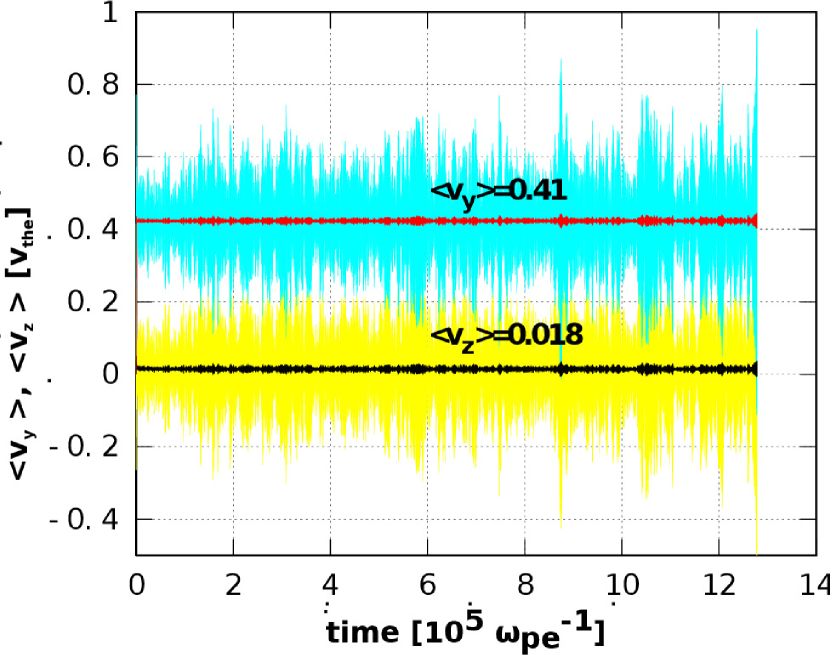
Figure 14: Time evolution of $\langle v_{y}\rangle$ (cyan) and $\langle v_{z}\rangle$ (yellow) of 1056 particles. The solid red line and the black line present the time average of the $\langle v_{y}\rangle$ and $\langle v_{z}\rangle$.

In Hall thrusters, it is experimentally observed Janes that the ratio of azimuthal to axial current-density $J_{y}/J_{z}\sim 10$. In our numerical study, we use 1056 particles with random initial positions in the rectangle $0\leq x_{0}\leq 2\pi/k_{1x}$, $0\leq y_{0}\leq 4\pi/k_{1y}$, $z_{0}=0$ and with velocities drawn from a 3D Gaussian distribution with unit standard-deviation along all three directions. We observe that the velocity distributions along $z$- and $y$-directions are nearly identical, therefore the number densities along these two directions are equal. We can compare the mean velocity ratio with the mean current density ratio along these two directions. Fig. 14 shows that $\langle v_{y}\rangle=0.41$ and $\langle v_{z}\rangle=0.018$, so that $\langle v_{y}\rangle/\langle v_{z}\rangle\sim 20$, which is of the same order as the experimental observation.

VI Conclusions

In this paper, we carried out model calculations to provide a dynamical basis for the high value of the experimentally observed anomalous cross-field transport in thruster configurations. The underlying mechanism is associated with the chaotic dynamics of electrons due to their interaction with a spectrum of unstable electrostatic waves. The electrostatic waves are generated due to the ${\mathbf{E}}\times{\mathbf{B}}$ electron drift instability. In the presence of a magnetic field $B_{0}$, an axial constant electric field $E_{0}$ and the electrostatic waves, the drifted cyclotron motion becomes chaotic due to the strong wave-particle interaction. In presence of more than one wave, the electrons gain energy over long time evolution and their temperature is increased along the perpendicular direction. This chaotic dynamics helps in the transport of electrons along the thruster axial direction.

A significant amount of axial electron transport is observed in presence of more than one wave, and the electrons exit from the thruster chamber. The reflection at boundary enhances the transport coefficient. The duration of wave-particle interaction depends on the ratio $\omega_{\mathrm{b}}/\omega_{\mathrm{c}}$ of bounce frequency to cyclotron frequency. With increase of amplitude and $k_{y}$ values of the background waves, the value of the bounce frequency increases, which enhances the energy exchange rate and the anomalous diffusion coefficient. The existence of harmonics in $k_{y}$ helps to generate different stochastic webs, which increases the diffusion coefficient. The average velocity ratio along azimuthal to axial direction $\langle v_{y}\rangle/\langle v_{z}\rangle$ in our numerical model is in good agreement with experimental observations.

References

- (1) A. I. Morozov and V. V. Savelyev, Rev. Plasma Phys. 21, 203 (2000).
- (2) G. S. Janes and R. S. Lowder, Phys. Fluids 9, 1115 (1966).
- (3) S. Tsikata, C. Honoré, N. Lemoine, D. M. Grésillon, Phys. Plasmas 17, 112110 (2010).
- (4) A. Smirnov, Y. Raitses and N. J. Fisch, Phys. Plasmas 14, 057106 (2007).
- (5) J. C. Adam, A. Héron, and G. Laval, Phys. Plasmas 11, 295 (2004).
- (6) T. Lafleur, S. D. Baalrud and P. Chabert, Phys. Plasmas 23, 053502 (2016).
- (7) J. P. Boeuf and L. Garrigues, Phys. Plasmas 25, 061204 (2018).
- (8) N. A. Marusov, E. A. Sorokina, V. P. Lakhin, V. I. Ilgisonis and A. I. Smolyakov, Plasma Sources Sci. Tech. 28, 015002 (2019).
- (9) J. C. Adam, J. P. Boeuf et al., Plasma Phys. Control. Fusion 50, 124041 (2008).
- (10) J. Cavalier, N. Lemoine, G. Bonhomme, S. Tsikata, C. Honoré and D. Grésillon, Phys. Plasmas 20, 082107 (2013).
- (11) P. S. Gary, J. Plasma Phys. 6, 561 (1971).
- (12) P. S. Gary and J.J. Sanderson, J. Plasma Phys. 4, 739 (1970).
- (13) A. B. Mikhailovskii, Electromagnetic instabilities in an inhomogeneous plasma, transl. E. W. Laing, Institute of Physics Publishing (Bristol, 1992).
- (14) S. N. Abolmasov, Plasma Sources Sci. Technol. 21, 035006 (2012).
- (15) J. P. Boeuf, J. Claustre, B. Chaudhury and G. Fubiani, Phys. Plasmas 19, 113510 (2012).
- (16) C. L. Ellison, Y. Raitses and N. J. Fisch, Phys. Plasmas 19, 013503 (2012).
- (17) M. Matsukuma, Th. Pierre, A. Escarguel, D. Guyomarc’h, G. Leclert, F. Brochard, E. Gravier and Y. Kawai, Phys. Lett. A 314, 163 (2003).
- (18) G. V. Gordeev, Zh. Eksp. Teor. Fiz. 23, 660 (1952) [Sov. Phys. JETP 6, 660 (1952)].
- (19) J. Boris, Proc. Fourth Conf. Numer. Simul. Plasmas, NRL, Washington, D.C., pp. 3-67 (1970).
- (20) Yu Daren, Li Hong and Wu Zhiwen Phys. Plasmas 14, 064505 (2007).
- (21) G. M. Zaslavsky, Chaos 1, 1 (1991).
- (22) X. Leoncini, C. Chandre and O. Ourrad, C. R. Mécanique 336, 530 (2008).
- (23) A. A. Vasil’ev and G. M. Zaslavskiĭ, Sov. Phys. JETP 72(5), 826 (1991).
- (24) MesoCentre, Aix-Marseille Université [https://mesocentre.univ-amu.fr/en/].