On the design of convolutional neural networks for automatic detection of Alzheimer’s disease

Abstract

Early detection is a crucial goal in the study of Alzheimer’s Disease (AD). In this work, we describe several techniques to boost the performance of 3D convolutional neural networks trained to detect AD using structural brain MRI scans. Specifically, we provide evidence that (1) instance normalization outperforms batch normalization, (2) early spatial downsampling negatively affects performance, (3) widening the model brings consistent gains while increasing the depth does not, and (4) incorporating age information yields moderate improvement. Together, these insights yield an increment of approximately 14% in test accuracy over existing models when distinguishing between patients with AD, mild cognitive impairment, and controls in the ADNI dataset. Similar performance is achieved on an independent dataset. We make our code and models publicly available at https://github.com/NYUMedML/CNN_design_for_AD.

1 Introduction

Alzheimer’s disease (AD) is the leading cause of dementia, and the 6th leading cause of death in the U.S. (National Center for Health Statistics (2017)). Unfortunately, all clinical trials to reverse AD have failed so far (Servick (2019)). It is hypothesized that clinical trials need to target patients at earlier stages before significant brain atrophies. But diagnosing the disease at an early stage is challenging. The current method for early detection relies on PET imaging, which is invasive and very costly. Various studies show that AD-related brain degeneration begins years before the clinical onset of symptoms (Jagust (2018)). This suggests that early detection of AD might be possible from standard structural brain imaging scans. Unfortunately, both clinical and also research-grade detection accuracies remain low.

In this paper we focus on learning to differentiate between cognitively normal aging (CN), mild cognitive impairment (MCI), and Alzheimer’s disease (AD), using structural brain MRI (T1-weighted scans). We propose a 3D convolutional neural network (CNN) architecture that achieves state-of-the-art performance for this task. The key novel components of the architecture are (1) instance normalization, an alternative to batch normalization introduced originally in the context of style transfer (Ulyanov et al. (2016); Huang and Belongie (2017)), (2) the use of small-sized kernels in the first layer to avoid downsampling, (3) wide architectures with large numbers of filters and relatively few layers, (4) providing the age of the patient to the network through an embedding inspired by a recent technique from natural language processing (Vaswani et al. (2017)).

Section 3 describes the data and our preprocessing scheme. Our methodology is then presented in Section 4. In Section 5 we report ablation experiments on the test set to isolate the effect of the different elements in our model, as well as additional analysis of the results. Code to reproduce our main results is publicly available at https://github.com/NYUMedML/CNN_design_for_AD.

2 Related Work

An important task in automatic diagnostics of AD is to distinguish patients with different degrees of mental impairment from MRI scans. Initial works applied simple classifiers such as support vector machines on features obtained from volumetric measurements of the hippocampus (Gerardin et al. (2009)) and other brain areas (Plant et al. (2010)).

More recently, several deep-learning approaches have been applied to this task. Gupta et al. (2013) used pretraining based on a sparse autoencoder to perform classification on the Alzheimer’s Disease Neuroimaging Initiative (ADNI) dataset (ADNI ). Hon and Khan (2017) applied state-of-the-art architectures such as VGG (Simonyan and Zisserman (2014)) and Inception Net (Szegedy et al. (2015)) on the OASIS dataset (Marcus et al. (2010)), selecting the most informative slices in the 3D scans based on image entropy. Valliani and Soni (2017), showed that a ResNet (He et al. (2016)) pretrained on ImageNet (Deng et al. (2009)) outperformed a baseline 2D CNN. Hosseini-Asl et al. (2016) evaluated a 3D CNN architecture on ADNI and data from the CADDementia challenge (Bron et al. (2015)). Cheng et al. (2017) proposed a more computationally-efficient approach based on large 3D patches processed by individual CNNs, which are then combined by an additional CNN to produce the output. Lian et al. (2018) proposed a related hierarchical CNN architecture that automatically identifies significant patches. Siamese networks were applied by Khvostikov et al. (2018) to distinguish regions of interest around the hippocampus fusing data from multiple imaging modalities.

As described in a recent survey paper, Wen et al. (2019), many existing works suffer from data leakage due to flawed data splits, biased transfer learning, or the absence of an independent test set. The authors also report that, in the absence of data leakage, CNNs achieve an accuracy of 72-86% when distinguishing between AD and healthy controls. In a similar spirit, Fung et al. (2019) studied the effect of different data-splitting strategies on classification accuracy. A significant drop in test accuracy (from 84% to 52% for the three-class classification problem considered in the present work) was reported when there was no patient overlap between the training and test sets. Bäckström et al. (2018) also studied the effect of splitting strategies and report similar results for two-way classification.

3 Datasets and Preprocessing

3.1 Datasets

For this study, we use T1-weighted structural MRI scans from the ADNI dataset (Mueller et al. (2005)), which have undergone specific image preprocessing steps including multiplanar reconstruction (MPR), Gradwarp, B1 non-uniformity correction, and N3 intensity normalization (ADNI (2008)). In total, we used over 3000 preprocessed scans. According to the ADNI procedures manuals, labels in the ADNI dataset are extracted based on the scores obtained on memory tasks– corrected by education level– and other criteria, some of which are subjective (ADNI (2008)). The labels are AD (mildly demented patients diagnosed with AD), MCI (mildly cognitively-impaired patients in the prodromal phase of AD) and CN (elderly control participants).

3.2 Data preprocessing

Most previous studies use packages such as FSL , Statistical Parametric Mapping (SPM ), and FreeSurfer (Fischl (2012)) to preprocess the data. FSL provides brain extraction and tissue segmentation functionality, while SPM realigns, spatially normalizes, and smooths the scans. FreeSurfer provides a preprocessing stream that includes skull stripping, segmentation, and nonlinear registration. For this study, we used the Clinica software platform developed by ARAMIS Lab , which supports FSL, SPM and FreeSurfer. We first split patients into training, validation and test sets. Then we use Clinica to register the scans to a Dartel template computed exclusively from the training data (Ashburner (2007)), and normalize them to the Montreal Neurological Institute (MNI) coordinate space (Evans et al. (1993)). The validation and test data are not used to compute any templates in order to avoid data leakage. The input to the Clinica software is the ADNI scans converted to BIDS format. The output dimensions are 121 $\times$ 145 $\times$ 121 voxels along sagittal, coronal and axial dimensions respectively. Due to preprocessing and registration errors, the final number of scans in our dataset is 2702.

The subjects in the dataset are split between training (70%), validation (15%) and test (15%) sets. As mentioned in the previous section, the split is carried out before preprocessing to avoid any data leakage. Data leakage resulting from using the same subjects in the training and test sets has been shown to artificially improve model performance by a large margin (Bäckström et al. (2018); Fung et al. (2019)). Table 1 shows the demographics of the patients in the training, validation, and test sets.

Split	Class	Num. subjects	Num. Scans	Mean Age (std)
Train	CN	140	567	77.0 (5.4)
	MCI	248	840	75.9 (7.3)
	AD	193	527	76.7 (7.4)
Val	CN	33	126	77.2 (5.6)
	MCI	39	138	73.3 (7.2)
	AD	41	124	76.1 (8.3)
Test	CN	24	105	79.0 (6.1)
	MCI	43	140	76.7 (6.5)
	AD	45	135	76.4 (5.1)

Table 1: Demographics of our training, validation and test sets after preprocessing.

4 Methodology

Figure 1 shows a scatterplot of the values of two popular hand-crafted features associated to AD diagnostics: normalized hippocampus volumes and entorhinal volumes (Frisoni et al. (1999); Leandrou et al. (2018)). The features are informative (AD patients tend to have smaller volumes with respect to healthy controls), but they do not enable accurate classification due to the significant overlap between the three classes. This motivates learning discriminative features automatically. Our proposed methodology achieves this using a deep convolutional neural network, inspired by their success in computer vision. However, it is worth emphasizing that our dataset of interest is very different to the datasets of natural images typically used to benchmark computer vision tasks. In our case, all scans are registered and have very similar structure. In addition, the number of examples is usually orders of magnitude smaller. Therefore, we need to design architectures capable of learning subtle differences from relatively small datasets.

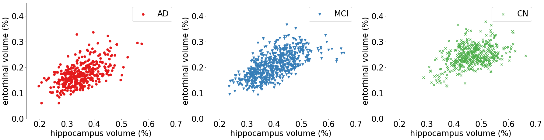
Figure 1: Visualization intracranial normalized hippocampus and entorhinal volumes of AD, MCI, and CN subjects. Note that there is significant overlap between the three classes.

4.1 Proposed model

Our proposed architecture is a 3D CNN model, composed of convolutional, normalization, activation and max-pooling layers. The architecture is described in more detail in Table 2. In this section, we outline several design choices that significantly boost the performance of the network for the task of differentiating between CN, AD, and MCI patients.

Instance normalization. Batch normalization, introduced by Ioffe and Szegedy (2015), has become one of the standard techniques to ease training of deep feed-forward networks. In our proposed model, however, we apply instance normalization, a technique introduced in the context of style transfer (Ulyanov et al. (2016); Huang and Belongie (2017)). In Section 5.3.1, we show that applying instance normalization consistently outperforms batch normalization for our task of interest.

Small-sized kernels. In contrast to most standard architectures for image classification, we use small-sized kernels in the first convolutional layer to prevent early spatial downsampling. For instance, ResNet and AlexNet use relatively large kernel sizes and strides in their first layer, which dramatically reduce the spatial dimension of their inputs. This accelerates the computation and is not usually detrimental in the case of natural-image classification tasks. However, for our task of interest, early downsampling results in significant loss of performance, as we show in Section 5.3.2.

Wider network. In our architecture design we favor a wider architecture that is not too deep. In Section 5.3.3, we find that increasing the depth of the model only brings marginal gains, whereas widening the architecture improves performance significantly.

Age encoding. Brains typically shrink to some degree in healthy aging (Peters (2006)). This might confuse the model since Alzheimer’s disease may have a similar effect (Van Hoesen et al. (1991)). A simple way to incorporate age in our model is to concatenate the normalized age of the patient to the output of the convolutional layers. However, this seems to result in worse performance. In order to better integrate age information, we encode each age value into a vector and combine the vector with the output of the convolutional layers. See Appendix A for further details.

Block	Layer	Type	Output size
	Inputs		$96\times 96\times 96$
1	Conv3D	k1-c4$\cdot f$-p0-s1-d1	$96\times 96\times 96$
	InstanceNorm3D
	ReLU
	MaxPool3D	k3-s2	$47\times 47\times 47$
2	Conv3D	k3-c32$\cdot f$-p0-s1-d2	$43\times 43\times 43$
	InstanceNorm3D
	ReLU
	MaxPool3D	k3-s2	$21\times 21\times 21$
3	Conv3D	k5-c64$\cdot f$-p2-s1-d2	$17\times 17\times 17$
	InstanceNorm3D
	ReLU
	MaxPool3D	k3-s2	$8\times 8\times 8$
4	Conv3D	k3-c64$\cdot f$-p1-s1-d2	$6\times 6\times 6$
	InstanceNorm3D
	ReLU
	MaxPool3D	k5-s2	$5\times 5\times 5$
FC1		1024
FC2		3
Softmax		3

Table 2: The backbone architecture. k = kernel size, c = number of channels as a multiple of the widening factor $f$, p = padding size, s = stride and d = dilation. We report results for $f$ equal to 1, 2, 4, and 8 in Section 5. The age encoding, if used, is forward propagated through two linear layers with layer normalization before being added to the output of FC1, see Table 6 in the Appendix for details.

5 Experiments and Results

In this section, we present and interpret the results of our study, which demonstrate the effectiveness of the techniques described in Section 4.

Method	Accuracy	Balanced Acc	Micro-AUC	Macro-AUC
ResNet-18$\star$	$50.8\%$	-	-	-
ResNet-18 pretrained$\star$	$56.8\%$	-	-	-
ResNet-18 3D$\diamond$	$52.4\pm 1.8\%$	$53.1\%$	-	-
ResNet-18 3D	$50.1\pm 1.1\%$	$51.3\pm 1.0\%$	$71.2\pm 0.4\%$	$72.4\pm 0.7\%$
AlexNet 3D	$57.2\pm 0.5\%$	$56.2\pm 0.8\%$	$75.1\pm 0.4\%$	$74.2\pm 0.5\%$
proposed$\bullet$	$66.9\pm 1.2\%$	$67.9\pm 1.1\%$	$82.0\pm 0.7\%$	$78.5\pm 0.7\%$
proposed$\bullet$  + Age	$\bf{68.2\pm 1.1}\%$	$\bf{70.0\pm 0.8\%}$	$\bf{82.0\pm 0.2\%}$	$\bf{80.0\pm 0.5\%}$

• Results on $2D$ ResNets initialized with or without pretrained weights on Imagenet reported by Valliani and Soni (2017).

• $3D$ ResNet with mild modifications, see Fung et al. (2019) for details. The balanced accuracy is computed using the confusion matrix in the paper.

• The backbone model showed in Table 2 with a widening factor of $8$.

Table 3: Comparison of the published models to our best proposed models. + Age means that the model incorporates age encodings.

Figure 2: ROC curves on the validation set (left) and test set (right). Differentiating CN or AD from all other classes results in high AUCs while detecting MCI remains a difficult task.

5.1 Description of computational experiments

We choose AlexNet and ResNet as baseline 3D CNNs since they are popular in computer vision as well as for our task. Unsurprisingly, given the size of the dataset, all architectures, including ResNet and AlexNet, are able to fit the training set with high balanced accuracy, while the generalization ability varies. We perform data augmentation via Gaussian blurring with $\sigma$ uniformly chosen from 0 to 1.5, and random cropping of size $96\times 96\times 96$. We set the batch size to 4 (for memory considerations) and the learning rate to 0.01. We use stochastic gradient descent with momentum equal to 0.9. We use the same settings for AlexNet and ResNet, except for the batch size which is set to 16 since these architectures use batch normalization. After training, the models with the lowest validation loss are saved and evaluated on the test set to obtain the results reported in Table 3. We compute the confidence intervals using bootstrapping.

5.2 Comparison to other methods

Our primary metric in this work is standard classification accuracy (Acc). As the test set is not necessarily balanced, we also use balanced classification accuracy (Bal-Acc) which is calculated as the average of the recall of each class. We also compute area under the ROC curves (AUCs), which are widely used for measuring the predictive accuracy of binary classification problems. This metric indicates the relationship between the true positive rate and false positive rate when the classification threshold varies. As AUC can only be computed for binary classification, we compute AUCs for all three binary problems of distinguishing between one of the categories and the rest. We also calculate micro and macro averages, denoted as Micro-AUC and Macro-AUC respectively.

Table 3 summarizes our results. Our proposed model significantly outperforms previously reported results, as well as the baseline architectures. Incorporating age through the proposed encoding improves performance moderately. We show the ROC curves obtained on the validation and test set in Figure 2. The model achieves around $90\%$ AUC when distinguishing CN or AD from the other two classes, and $60-65\%$ when distinguishing MCI from the other two classes.

5.3 Ablation studies

In this section, we perform ablation studies on the techniques described in Section 4 to isolate their individual contributions to the accuracy of the proposed model. The studies were performed on the test set.

5.3.1 Instance normalization vs batch normalization

We compare batch normalization (BN) and instance normalization (IN) on the backbone architecture using different widening factors and on ResNet-18. The results are in Table 4. More comprehensive evaluations on different widening factors are presented in Table 8 of Appendix B. Models with IN layers perform consistently better than models with BN layers.

Method	Accuracy	balanced Acc	Micro-AUC	Macro-AUC
$\times 4$ with IN	$\bf{63.2\pm 1.0\%}$	$\bf{63.3\pm 0.9\%}$	$\bf{80.5\pm 0.5\%}$	$\bf{77.0\pm 0.7\%}$
$\times 4$ with BN	$61.8\pm 1.1\%$	$62.2\pm 1.1\%$	$77.0\pm 0.5\%$	$73.0\pm 0.6\%$
$\times 8$ with IN	$\bf{66.9\pm 1.2\%}$	$\bf{67.9\pm 1.1\%}$	$\bf{82.0\pm 0.7\%}$	$\bf{78.5\pm 0.7\%}$
$\times 8$ with BN	$58.8\pm 0.9\%$	$60.7\pm 0.7\%$	$75.9\pm 0.7\%$	$73.1\pm 0.8\%$
ResNet-18 with IN	$\bf{52.3\pm 0.8\%}$	$\bf{52.7\pm 1.1\%}$	$\bf{74.1\pm 0.7\%}$	$\bf{73.1\pm 0.9\%}$
ResNet-18 with BN	$50.1\pm 1.1\%$	$51.3\pm 1.0\%$	$71.2\pm 0.4\%$	$72.4\pm 0.7\%$

Table 4: Comparison of batch normalization (BN) and instance normalization (IN) layers on the backbone architecture with widening factor of 4 and 8 and on ResNet-18. See also Table 8 for results with other widening factors. Instance normalization outperforms batch normalization in all cases.

5.3.2 Early spatial downsampling

Here we study how the kernel size of the first convolutional layer affects the final classification performance. We compare original kernel sizes $1\times 1\times 1$ with stride 1, $3\times 3\times 3$ with stride 2, and $7\times 7\times 7$ with stride 4. The results are summarized in Figure 3. The smallest kernel has the best performance. This is a possible explanation for the inferior performance of ResNet and AlexNet for our task. We further check this hypothesis for ResNet, the results show that reducing kernel size for the initial layer is effective for ResNet as well (see details in Appendix C).

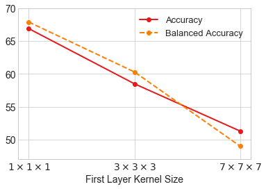
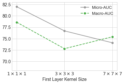
Figure 3: Comparison of the performances of different first layer kernel sizes for the backbone architecture in Table 2. Larger kernel sizes in the first layer result in worse performance.

5.3.3 Wider or deeper model?

In this section we compare the effect of varying width or depth on classification accuracy. The left graph in Figure 4 shows that widening the network architecture leads to better classification performance up until a certain point. This finding is in line with results reported for the ResNet by Zagoruyko and Komodakis (2016). We increase the depth of our backbone network by adding convolutional blocks (convolutional layers + instance normalization + ReLU activation). It should be noted that the size of the representation output from the final convolutional block might decrease when the network becomes deeper. To control for the effects of the representation size when making the architecture deeper, convolutional layers in each block are set to have kernel size of $3\times 3\times 3$, stride of 1 and padding of 1. Increasing depth only achieves small gains in accuracy. We also observe that deeper networks are often slower and more difficult to train when compared to wider networks.

Width	Depth

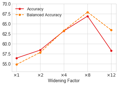
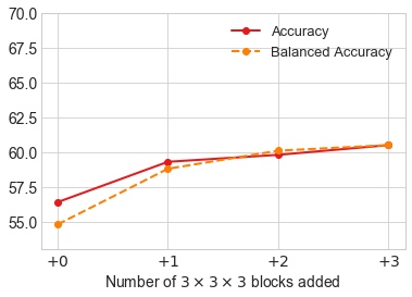
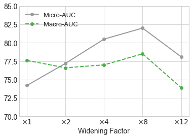
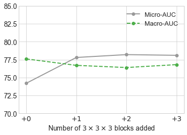
Figure 4: Performance for different widening factors (left) and numbers of added blocks (right) for backbone architecture in Table 2. Wider architectures consistently achieve better performance up until a widening factor of x4. Deeper networks only achieve marginal improvement.

5.3.4 Impact of dataset size

In Figure 5, we report the performance of the proposed model for datasets of different sizes (obtained by randomly subsampling the data). We observe that increasing the size of the dataset results in better performance in all evaluation metrics. Given that the model is trained on a very small dataset compared to regular computer-vision tasks, more data may be needed to exhaust the representation ability of the models.

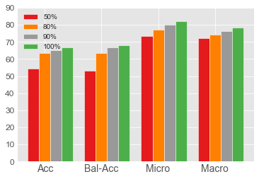
Figure 5: Performance of the proposed model evaluated using different subsampling rates. The trend is clear: increasing dataset size improves performance across all evaluation metrics.

5.4 Validation with independent dataset

We test the generalization capacity of our model on a completely separate dataset, obtained from the Australian Imaging Biomarkers and Lifestyle flagship study of ageing (AIBL) (Ellis et al. (2009)). We follow the same preprocessing procedures as for the ADNI validation and test set (described in Section 3), being careful to avoid any data leakage. After preprocessing, we obtain 783 CN scans from 461 subjects with average age 73.5, 150 MCI scans from 113 subjects with average age 76.2, and 134 AD scans from 95 subjects with average age 75.4. The results are shown in Table 5. We apply our proposed architecture without age information, since this information may not be readily available for different datasets. The model achieves a similar performance on this independent dataset as on the ADNI data, which demonstrates that the features learned by the network generalize effectively.

Method	Accuracy	Balanced Acc	Micro-AUC	Macro-AUC
proposed on ADNI	$66.9\pm 1.2\%$	$67.9\pm 1.1\%$	$82.0\pm 0.7\%$	$78.5\pm 0.7\%$
proposed on AIBL	$63.6\pm 0.7\%$	$65.7\pm 1.1\%$	$90.0\pm 0.6\%$	$82.1\pm 0.7\%$

Table 5: Comparison of the performance of the proposed model on the ADNI and AIBL datasets.

6 Analysis

6.1 Analysis of wrongly-classified subjects

We analyze the wrongly-classified validation examples in Figure 6. Mini-Mental State Exam (MMSE) scores (with value ranges from 0 to 30) are widely used tools for detecting cognitive impairment, assessing severity, and monitoring cognitive changes over time. Lower scores often mean more cognitive impairment. The model’s output after the softmax layer (logits) can be viewed as the confidence of the model in predicting a class. The trend in the figure shows that for higher MMSE scores the model becomes more confident in predicting CN, and less confident in predicting AD. Since the criteria to assign labels are subjective, and the boundary between MCI and the other two classes is not always clear, it is possible that some of the classification errors are due to noise in the labels.

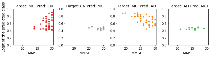
Figure 6: The Mini-Mental State Exam (MMSE) scores and corresponding logits of the predicted class for wrongly-classified validation examples.

6.2 Opening the black box

In order to visualize the features learned by the model, we compute saliency maps consisting of the magnitude of the gradient of the target class score with respect to the input (Simonyan et al. (2013)). Figure 7 shows examples of these saliency maps for randomly selected scans in the validation set belonging to each class. It also shows aggregated maps that combine saliency maps from all scans in the validation set. These results reveal some interesting aspects of the proposed model: the model focuses on gray-matter regions around the hippocampus and the ventricles, which is consistent with existing biomarkers (Risacher and Saykin (2013)), as well as on some additional regions. A detailed study of these regions lies beyond the scope of this work, but is an intriguing direction for future research.

	Axial 50th	Axial 26th	Coronal 56th	Sagittal 26th
Agg.
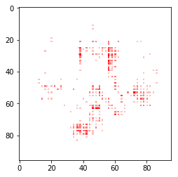
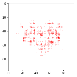
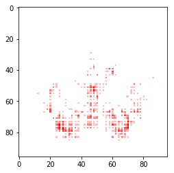
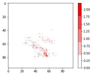
CN
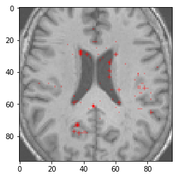
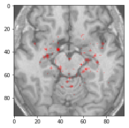
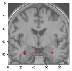
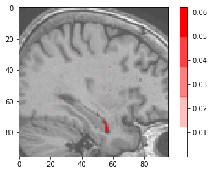
MCI
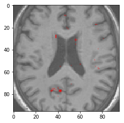
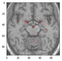
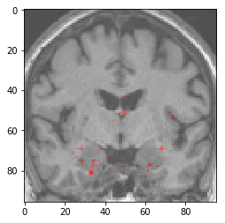
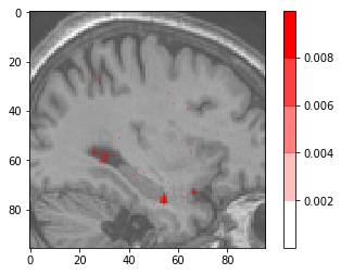
AD

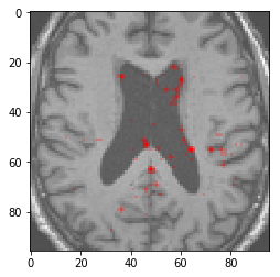
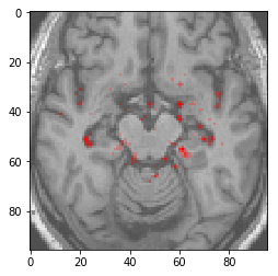
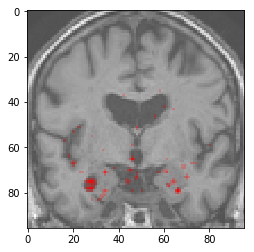
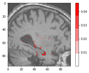
Figure 7: Visualization of class saliency maps (slices) obtained by computing the magnitude of the gradient of the learned map associated to each class with respect to the input (for each patient we compute the gradient with respect to their true class). The top row shows a aggregated plot of all saliency maps in the validation set for three slices. The bottom rows show saliency maps for examples of patients in each class superposed on the corresponding registered brain scan and smoothed by a Gaussian kernel with $\sigma=0.8$.

7 Conclusion

In this paper, we develop a novel 3D CNN architecture to perform three-way classification between patients with Alzheimer’s disease, patients with mild cognitive impairment, and healthy controls. Our architecture combines different elements (instance normalization, wider layers, and an encoding of the patient’s age) to achieve a significant gain in classification accuracy, demonstrated on completely held-out data and on an independent dataset.

The authors would like to thank Henry Rusinek and Arjun Masurkar for their useful comments on earlier versions of this manuscript. Authors also acknowledge Leon Lowenstein Foundation for funding support, and the Alzheimer’s Disease Neuroimaging Initiative (ADNI) (National Institutes of Health Grant U01 AG024904) and DOD ADNI (Department of Defense award number W81XWH-12-2-0012), as well as National Institute on Aging and the National Institute of Biomedical Imaging and Bioengineering for data collection and sharing.

Appendix A Age encodings

To compute the age encoding vector, we first fix the age values range from 0 to 120 years old, and round all possible age values to 0.5 decimal places. In total, we get 240 possible age values. Inspired by the positional encoding in the transformer model (Vaswani et al. (2017)), we use sinusoidal functions to implement the encoding. We define $\text{AE}_{(\text{age})}\in\mathbf{R}^{d_{\text{model}}}$ to be the age encoding function defined as:

$$\text{AE}_{(\text{age},2i)} =\sin(\text{age}/10000^{2i/d_{\text{model}}})$$

$$\text{AE}_{(\text{age},2i+1)} =\cos(\text{age}/10000^{2i/d_{\text{model}}})$$

where age is one of the 240 possible age values,and $i=0,1,2,\dots,d_{\text{model}}/2-1$ is the dimension and $d_{\text{model}}$ is the size of the encodings. We further transform the age encodings using a few fully connected layers to match the scales and sizes with the visual representation. The architecture for the transformation is showed in Table 6.

Layer	Output size
Linear	512
LayerNorm	512
Linear	1024

Table 6: The age encoder architecture

We compare this method with a simple baseline. In the baseline, we directly concatenate normalized age (with range from 0 to 1) to the learned representation obtained from the convolutional layers. The results are in Table 7. Our proposed encoding results in improved performance, whereas the baseline encoding results in worse performance.

Method	Accuracy	Balanced Acc	Micro-AUC	Macro-AUC
No age information	$66.9\pm 1.2\%$	$67.9\pm 1.1\%$	$82.0\pm 0.7\%$	$78.5\pm 0.7\%$
Proposed age encoding	$\bf{68.2\pm 1.1}\%$	$\bf{70.0\pm 0.8\%}$	$\bf{82.0\pm 0.2\%}$	$\bf{80.0\pm 0.5\%}$
Baseline age encoding	$61.5\pm 1.4\%$	$62.6\pm 1.0\%$	$78.6\pm 1.2\%$	$78.3\pm 1.1\%$

Table 7: Comparison of different ways of incorporating the age information using the proposed architecture.

Appendix B Instance Normalization vs Batch Normalization

In Table 8, we present the complete results of comparing Instance Normalization (IN) and Batch Normalization (BN) on our backbone architecture with various widening factors. IN consistently outperforms BN for all architectures.

Method	Accuracy	balanced Acc	Micro-AUC	Macro-AUC
$\times 1$ with IN	$\bf{56.4\pm 1.4\%}$	$\bf{54.8\pm 1.2\%}$	$\bf{74.2\pm 0.8\%}$	$\bf{75.6\pm 0.9\%}$
$\times 1$ with BN	$54.2\pm 1.2\%$	$53.3\pm 0.8\%$	$74.1\pm 0.7\%$	$73.2\pm 0.9\%$
$\times 2$ with IN	$\bf{58.4\pm 1.7\%}$	$\bf{57.8\pm 1.7\%}$	$\bf{77.2\pm 0.8\%}$	$\bf{76.6\pm 0.9\%}$
$\times 2$ with BN	$57.1\pm 0.7\%$	$55.6\pm 0.8\%$	$74.8\pm 0.6\%$	$73.6\pm 0.6\%$
$\times 4$ with IN	$\bf{63.2\pm 1.0\%}$	$\bf{63.3\pm 0.9\%}$	$\bf{80.5\pm 0.5\%}$	$\bf{77.0\pm 0.7\%}$
$\times 4$ with BN	$61.8\pm 1.1\%$	$62.2\pm 1.1\%$	$77.0\pm 0.5\%$	$73.0\pm 0.6\%$
$\times 8$ with IN	$\bf{66.9\pm 1.2\%}$	$\bf{67.9\pm 1.1\%}$	$\bf{82.0\pm 0.7\%}$	$\bf{78.5\pm 0.7\%}$
$\times 8$ with BN	$58.8\pm 0.9\%$	$60.7\pm 0.7\%$	$75.9\pm 0.7\%$	$73.1\pm 0.8\%$
ResNet-18 with IN	$\bf{52.3\pm 0.8\%}$	$\bf{52.7\pm 1.1\%}$	$\bf{74.1\pm 0.7\%}$	$\bf{73.1\pm 0.9\%}$
ResNet-18 with BN	$50.1\pm 1.1\%$	$51.3\pm 1.0\%$	$71.2\pm 0.4\%$	$72.4\pm 0.7\%$

Table 8: Comparison of batch normalization (BN) and instance normalization (IN) layers on the backbone architecture with different widening factors as well as on ResNet-18, instance normalization outperforms batch normalization in all cases.

Appendix C Early spatial downsampling

Figure 8: Performance of different first layer kernel sizes for a ResNet-18 with IN. Method $\mathbf{(a)}$ modifying the kernel into $3\times 3\times 3$, stride 1. In method $\mathbf{(b)}$, we further add a $1\times 1\times 1$ convolutional block on the top of the model from method $\mathbf{(a)}$.

Figure 8 shows results for ResNet when for different kernel sizes of the first convolutional layer. We modify the architecture of a ResNet-18 with instance normalization in the following way: (a) we reduce the size of the first convolution from $7\times 7\times 7$ with stride 2 into $3\times 3\times 3$ with stride 1, (b) we further add a $1\times 1\times 1$ convolutional block on the top (right after the input), the results are showed in Figure 8. These results demonstrate that reducing filter size in the first convolutional layer yields performance improvements for the ResNet as well. For a ResNet-18 with batch normalization, performance also improves, although less markedly.

References

- (1) FMRIB software library. https://fsl.fmrib.ox.ac.uk/fsl. released: 2019-03-11.
- (2) Statistical parametric mapping. www.fil.ion.ucl.ac.uk/spm/. released: 2014-10-01.
- (3) ADNI. ADNI website. http://adni.loni.usc.edu/.
- ADNI (2008) ADNI. Alzheimer’s disease neuroimaging initiative 2 procedures manual, 2008.
- (5) ARAMIS Lab. Aramis lab. www.aramislab.fr.
- Ashburner (2007) John Ashburner. A fast diffeomorphic image registration algorithm. Neuroimage, 38(1):95–113, 2007.
- Bäckström et al. (2018) Karl Bäckström, Mahmood Nazari, Irene Yu-Hua Gu, and Asgeir Store Jakola. An efficient 3D deep convolutional network for Alzheimer’s disease diagnosis using MR images. In 2018 IEEE 15th International Symposium on Biomedical Imaging (ISBI 2018), pages 149–153. IEEE, 2018.
- Bron et al. (2015) Esther E Bron, Marion Smits, Wiesje M Van Der Flier, Hugo Vrenken, Frederik Barkhof, Philip Scheltens, Janne M Papma, Rebecca ME Steketee, Carolina Méndez Orellana, Rozanna Meijboom, et al. Standardized evaluation of algorithms for computer-aided diagnosis of dementia based on structural MRI: the caddementia challenge. NeuroImage, 111:562–579, 2015.
- Cheng et al. (2017) Danni Cheng, Manhua Liu, Jianliang Fu, and Yaping Wang. Classification of MR brain images by combination of multi-CNNs for AD diagnosis. In Ninth International Conference on Digital Image Processing (ICDIP 2017), volume 10420, page 1042042. International Society for Optics and Photonics, 2017.
- (10) Clinica. Clinica software platform. http://www.clinica.run. released: 2019-05-23.
- Deng et al. (2009) Jia Deng, Wei Dong, Richard Socher, Li-Jia Li, Kai Li, and Li Fei-Fei. Imagenet: A large-scale hierarchical image database. In 2009 IEEE conference on computer vision and pattern recognition, pages 248–255. Ieee, 2009.
- Ellis et al. (2009) Kathryn A Ellis, Ashley I Bush, David Darby, Daniela De Fazio, Jonathan Foster, Peter Hudson, Nicola T Lautenschlager, Nat Lenzo, Ralph N Martins, Paul Maruff, et al. The Australian Imaging, Biomarkers and Lifestyle (AIBL) study of aging: methodology and baseline characteristics of 1112 individuals recruited for a longitudinal study of Alzheimer’s disease. International Psychogeriatrics, 21(4):672–687, 2009.
- Evans et al. (1993) Alan C Evans, D Louis Collins, SR Mills, ED Brown, RL Kelly, and Terry M Peters. 3D statistical neuroanatomical models from 305 MRI volumes. In 1993 IEEE conference record nuclear science symposium and medical imaging conference, pages 1813–1817. IEEE, 1993.
- Fischl (2012) Bruce Fischl. Freesurfer. Neuroimage, 62(2):774–781, 2012.
- Frisoni et al. (1999) GB Frisoni, MP Laakso, A Beltramello, C Geroldi, A Bianchetti, H Soininen, and M Trabucchi. Hippocampal and entorhinal cortex atrophy in frontotemporal dementia and Alzheimer’s disease. Neurology, 52(1):91–91, 1999.
- Fung et al. (2019) Yi Ren Fung, Ziqiang Guan, Ritesh Kumar, Joie Yeahuay Wu, and Madalina Fiterau. Alzheimer’s disease brain MRI classification: Challenges and insights. arXiv preprint arXiv:1906.04231, 2019.
- Gerardin et al. (2009) Emilie Gerardin, Gaël Chételat, Marie Chupin, Rémi Cuingnet, Béatrice Desgranges, Ho-Sung Kim, Marc Niethammer, Bruno Dubois, Stéphane Lehéricy, Line Garnero, et al. Multidimensional classification of hippocampal shape features discriminates Alzheimer’s disease and mild cognitive impairment from normal aging. Neuroimage, 47(4):1476–1486, 2009.
- Gupta et al. (2013) Ashish Gupta, Murat Ayhan, and Anthony Maida. Natural image bases to represent neuroimaging data. In International conference on machine learning, pages 987–994, 2013.
- He et al. (2016) Kaiming He, Xiangyu Zhang, Shaoqing Ren, and Jian Sun. Deep residual learning for image recognition. In Proceedings of the IEEE conference on computer vision and pattern recognition, pages 770–778, 2016.
- Hon and Khan (2017) Marcia Hon and Naimul Mefraz Khan. Towards Alzheimer’s disease classification through transfer learning. In 2017 IEEE International Conference on Bioinformatics and Biomedicine (BIBM), pages 1166–1169. IEEE, 2017.
- Hosseini-Asl et al. (2016) Ehsan Hosseini-Asl, Georgy Gimel’farb, and Ayman El-Baz. Alzheimer’s disease diagnostics by a deeply supervised adaptable 3D convolutional network. arXiv preprint arXiv:1607.00556, 2016.
- Huang and Belongie (2017) Xun Huang and Serge Belongie. Arbitrary style transfer in real-time with adaptive instance normalization. In Proceedings of the IEEE International Conference on Computer Vision, pages 1501–1510, 2017.
- Ioffe and Szegedy (2015) Sergey Ioffe and Christian Szegedy. Batch normalization: Accelerating deep network training by reducing internal covariate shift. arXiv preprint arXiv:1502.03167, 2015.
- Jagust (2018) William Jagust. Imaging the evolution and pathophysiology of Alzheimer disease. Nature Reviews Neuroscience, 19(11):687, 2018.
- Khvostikov et al. (2018) Alexander Khvostikov, Karim Aderghal, Jenny Benois-Pineau, Andrey Krylov, and Gwenaelle Catheline. 3D CNN-based classification using sMRI and MD-DTI images for Alzheimer disease studies. arXiv preprint arXiv:1801.05968, 2018.
- Leandrou et al. (2018) Stephanos Leandrou, I Mamais, Styliani Petroudi, Panicos A Kyriacou, Constantino Carlos Reyes-Aldasoro, and Constantinos S Pattichis. Hippocampal and entorhinal cortex volume changes in Alzheimer’s disease patients and mild cognitive impairment subjects. In 2018 IEEE EMBS International Conference on Biomedical & Health Informatics (BHI), pages 235–238. IEEE, 2018.
- Lian et al. (2018) Chunfeng Lian, Mingxia Liu, Jun Zhang, and Dinggang Shen. Hierarchical fully convolutional network for joint atrophy localization and Alzheimer’s disease diagnosis using structural MRI. IEEE transactions on pattern analysis and machine intelligence, 2018.
- Marcus et al. (2010) Daniel S Marcus, Anthony F Fotenos, John G Csernansky, John C Morris, and Randy L Buckner. Open access series of imaging studies: longitudinal MRI data in nondemented and demented older adults. Journal of cognitive neuroscience, 22(12):2677–2684, 2010.
- Mueller et al. (2005) Susanne G Mueller, Michael W Weiner, Leon J Thal, Ronald C Petersen, Clifford R Jack, William Jagust, John Q Trojanowski, Arthur W Toga, and Laurel Beckett. Ways toward an early diagnosis in Alzheimer’s disease: the Alzheimer’s disease neuroimaging initiative (ADNI). Alzheimer’s & Dementia, 1(1):55–66, 2005.
- National Center for Health Statistics (2017) . National Center for Health Statistics. Deaths and mortality, May 2017. URL https://www.cdc.gov/nchs/fastats/deaths.htm. [Online; posted 07-May-2017].
- Peters (2006) Ruth Peters. Ageing and the brain. Postgraduate medical journal, 82(964):84–88, 2006.
- Plant et al. (2010) Claudia Plant, Stefan J Teipel, Annahita Oswald, Christian Böhm, Thomas Meindl, Janaina Mourao-Miranda, Arun W Bokde, Harald Hampel, and Michael Ewers. Automated detection of brain atrophy patterns based on MRI for the prediction of Alzheimer’s disease. Neuroimage, 50(1):162–174, 2010.
- Risacher and Saykin (2013) Shannon L Risacher and Andrew J Saykin. Neuroimaging and other biomarkers for Alzheimer’s disease: the changing landscape of early detection. Annual review of clinical psychology, 9:621–648, 2013.
- Servick (2019) K Servick. Another major drug candidate targeting the brain plaques of Alzheimer’s disease has failed. what’s left. Science, 10, 2019.
- Simonyan and Zisserman (2014) Karen Simonyan and Andrew Zisserman. Very deep convolutional networks for large-scale image recognition. arXiv preprint arXiv:1409.1556, 2014.
- Simonyan et al. (2013) Karen Simonyan, Andrea Vedaldi, and Andrew Zisserman. Deep inside convolutional networks: Visualising image classification models and saliency maps. arXiv preprint arXiv:1312.6034, 2013.
- Szegedy et al. (2015) Christian Szegedy, Wei Liu, Yangqing Jia, Pierre Sermanet, Scott Reed, Dragomir Anguelov, Dumitru Erhan, Vincent Vanhoucke, and Andrew Rabinovich. Going deeper with convolutions. In Proceedings of the IEEE conference on computer vision and pattern recognition, pages 1–9, 2015.
- Ulyanov et al. (2016) Dmitry Ulyanov, Andrea Vedaldi, and Victor Lempitsky. Instance normalization: The missing ingredient for fast stylization. arXiv preprint arXiv:1607.08022, 2016.
- Valliani and Soni (2017) Aly Valliani and Ameet Soni. Deep residual nets for improved Alzheimer’s diagnosis. In BCB, page 615, 2017.
- Van Hoesen et al. (1991) Gary W Van Hoesen, Bradley T Hyman, and Antonio R Damasio. Entorhinal cortex pathology in Alzheimer’s disease. Hippocampus, 1(1):1–8, 1991.
- Vaswani et al. (2017) Ashish Vaswani, Noam Shazeer, Niki Parmar, Jakob Uszkoreit, Llion Jones, Aidan N Gomez, Łukasz Kaiser, and Illia Polosukhin. Attention is all you need. In Advances in neural information processing systems, pages 5998–6008, 2017.
- Wen et al. (2019) Junhao Wen, Elina Thibeau-Sutre, Jorge Samper-Gonzalez, Alexandre Routier, Simona Bottani, Stanley Durrleman, Ninon Burgos, and Olivier Colliot. Convolutional neural networks for classification of Alzheimer’s disease: Overview and reproducible evaluation. arXiv preprint arXiv:1904.07773, 2019.
- Zagoruyko and Komodakis (2016) Sergey Zagoruyko and Nikos Komodakis. Wide residual networks. arXiv preprint arXiv:1605.07146, 2016.