Characterizing dynamically varying acoustic scenes from egocentric audio recordings in workplace setting

Abstract

Devices capable of detecting and categorizing acoustic scenes have numerous applications such as providing context-aware user experiences. In this paper, we address the task of characterizing acoustic scenes in a workplace setting from audio recordings collected with wearable microphones. The acoustic scenes, tracked with Bluetooth transceivers, vary dynamically with time from the egocentric perspective of a mobile user. Our dataset contains experience sampled long audio recordings collected from clinical providers in a hospital, who wore the audio badges during multiple work shifts. To handle the long egocentric recordings, we propose a Time Delay Neural Network (TDNN)-based segment-level modeling. The experiments show that TDNN outperforms other models in the acoustic scene classification task. We investigate the effect of primary speaker’s speech in determining acoustic scenes from audio badges, and provide a comparison between performance of different models. Moreover, we explore the relationship between the sequence of acoustic scenes experienced by the users and the nature of their jobs, and find that the scene sequence predicted by our model tend to possess similar relationship. The initial promising results reveal numerous research directions for acoustic scene classification via wearable devices as well as egocentric analysis of dynamic acoustic scenes encountered by the users.

Index Terms—  Acoustic scene classification, audio event detection, dynamic audio environment, time delay neural network

1 Introduction

Audio modality often provides information streams that are important in building multi-modal systems such as for enabling context-aware and personalized user experiences. There is a fast-growing research interest in building systems capable of understanding the ambient acoustic environment: this includes both its dynamically evolving nature in a given location, and across locations such as from the view point of a mobile user. An “acoustic scene” [1] refers to an audio environment characterized by the “sound events” [2] that occur in it. Machines with the ability of identifying the acoustic scene in a given audio recording have numerous applications in robot navigation [1, 3], context-aware devices and associated user notifications, advanced gaming systems, accessibility systems, self-driving vehicles, and surveillance [4]. The machine learning task of identifying the acoustic environment in an audio recording is generally known as Acoustic Scene Classification (ASC) [1]. Over the past few years, significant progress has been made in this domain of research in the form of new datasets (e.g., the DCASE challenges [5]) and novel algorithms [5, 6, 7, 8, 9].

Acoustic scenes can vary in granularity of their semantic descriptors, and they can be heterogeneous in nature [10, 11, 12] – location (indoor, outdoor, etc.), sources (alarms, chatter, door slams, etc.) and so on. For example, the acoustic environment of a workplace such as a hospital can have multiple sub-categories (acoustic locales) of interest such as nurse stations, medication rooms, patient rooms, labs, lounges, etc., each with distinct acoustic ambiences. Moreover, from the perspective of the employees in a workplace, the dynamically varying acoustic environments might look different for different job-types. A nurse in a hospital setting might experience most of the above acoustic scenes in a certain work shift as compared to a lab technician for instance. Identifying such dynamically changing acoustic scenes from an egocentric (centered around a certain person) view of the user, and characterizing their temporal patterns can potentially provide insights about the relationship between the acoustic scenes experienced by the employees and nature of their jobs. For example, stress patterns related to acoustic environments could be mapped.

In this paper, we address the task of identifying and characterizing dynamically varying acoustic scenes in a workplace setting from egocentric audio recordings obtained through audio recorders worn as badges by individuals [13]. There are three fundamental differences between the task at hand and standard ASC tasks [1, 6]. First, to get an egocentric view, we employ wearable microphones for audio feature collection [13]. The employees wear their audio recorders throughout multiple work shifts. The audio badges always capture the voice of the participant wearing the microphone; the speech is recorded at a higher intensity than the background scenes because of the sensor design. Second, from the standpoint of the participant, the acoustic scenes might vary dynamically over time (including across locations for ambulatory individuals such as nurses). Third, the acoustic scenes are from fine-grained classes inside the umbrella of a workplace (more specifically, a large critical care hospital) setting.

The main contributions of the paper are summarized below.

• This work formulates the problem of identifying dynamically varying acoustic scenes in a real world workplace setting.

• The data collection setup makes this a one of a kind problem as we have an unobtrusive, experience sampled [14] measurements of location and audio from an egocentric point of view.

• The present ASC task is constrained with the possible overlay of the user’s speech; acoustic scenes have to be identified even when the user is talking.

• The effect of foreground speech (the speaker wearing the audio badge) in predicting acoustics scenes from wearable microphones is analyzed.

• A deep learning framework based on a Time Delay Neural Network (TDNN) [15] model to learn the segment-level acoustic scenes from audio features is proposed.

• The temporal characteristics of the acoustic scenes experienced by the users are analyzed with respect to the nature of their occupations.

2 Dataset

The present work is a part of the “TILES: Tracking IndividuaL performancE with Sensors” project, which is a part of the IARPA MOSAIC program. The goal of this project is to assess the effect of multiple stressors (stressful events in life [16]) on workplace behaviors, affect, and performance of the employees through the use of off-the-shelf wearable sensors. We collected multi-modal sensory data (audio, physiology, continuous location, etc.) from $350$ nurses and other direct clinical providers in a critical care hospital. The data was collected through audio badges [13] developed in-house, which the participants wore during their work shifts. Each participant went through the data collection procedure in multiple work shifts, each typically lasted from $8$ to $12$ hours. The entire dataset was collected over the period of ten weeks. The dataset contains multiple days of multi-modal data for every participant, thus contains data with longer temporal context as compared to standard ASC tasks like [5]. This rich context inspired us to deploy segment-level modeling as described in Section 3. More details about the dataset can be found in [17]. For this work (in the initial phase), we employ a subset of $86$ participants ($29$ males and $57$ females).

2.1 Acoustic features

In compliance with HIPAA regulations [18] and because of the sensitive nature of the study environment (hospital), we were unable to collect raw audio signal. The audio badge [13], equipped with an energy based voice activity detector, collected $125$ low-level descriptor features using the OpenSMILE toolkit [19] at a sampling rate of $16$ kHz. The features were computed using a moving window of $60$ ms length with $50$ ms overlap [20]. The feature set consists of spectral features such as MFCCs, other speech features including pitch and loudness, and voice quality measures like vocal shimmer and jitter. We incorporate all features for our current analysis.

2.2 Acoustic scene location labels

The acoustic scene locales are derived from Bluetooth transceivers installed in different locations in the hospital [21] as a part of the TILES study. The transceivers receive Bluetooth pings sent by the audio badges, and provide Received Signal Strength Indicator (RSSI) values which are used to track the temporally varying acoustic environment from the participant’s perspective. The temporal resolution of this location data is much coarser ($\sim 1$ minute) than that of the acoustic features, and this needs further alignment step as discussed in Section 4.1. At every timestamp, maximum RSSI value is used to determine the fine-grained location of the participant. We refer the readers to [21] for further details about the indoor localization process. The fine-grained locations are then processed and clustered according to their associated acoustic environments. In this work, we target four different locations (see Figure 1) in a hospital unit, each having unique characteristics in their acoustic scenes: nurse stations (‘ns’), patient rooms (‘pat’), medication rooms (‘med’), and lounge (‘lounge’).

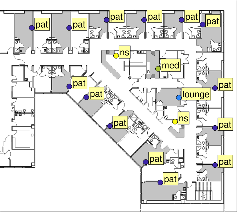
(a) Typical Floor plan.

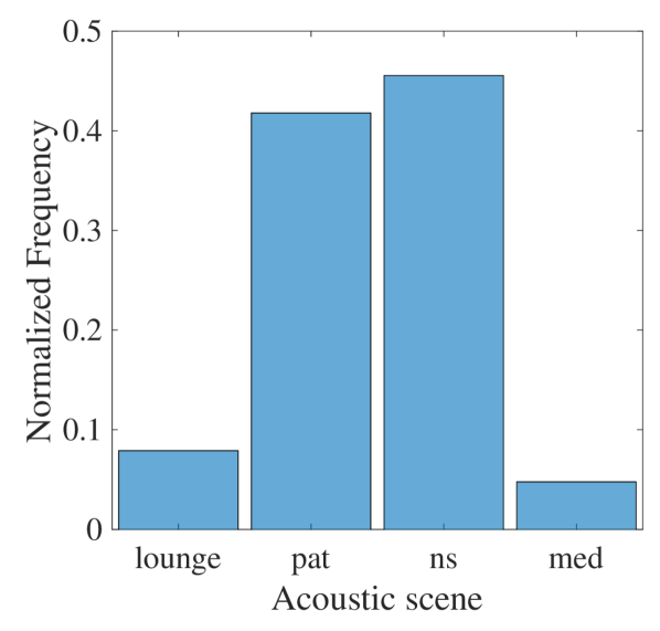
(b) Histogram of scenes.

Fig. 1: (a) One of the hospital floor plans showing different acoustic locales. (b) Histogram of acoustic scene samples in our dataset.

3 Methodology

Because of the having extremely long audio recordings for every participant (see Section 2), we address the problem with a segment-level modeling. The goal is to learn an acoustic scene model that can predict the scene given an input audio (features) segment. Moreover, we characterize the temporal sequence of predicted acoustic scenes for the subsequent analysis of its relationship with the nature of job..

3.1 Problem Formulation

Let, $\mathcal{D}=\left\{\mathcal{X}_{i},\mathcal{Y}_{i}\right\}_{i=1}^{N}$ be a dataset of $N$ participants. Here $\mathcal{X}_{i}$ denotes the temporal sequence of segmented audio features for the $i^{\text{th}}$ participant:

$$\mathcal{X}_{i}=\left[\mathbf{X}_{i1},\mathbf{X}_{i2},\dots,\mathbf{X}_{iT_{i}}\right].$$ (1)

Here, $\mathbf{X}_{ij}\in\mathbb{R}^{L_{ij}\times F}$ denotes the $j^{\text{th}}$ segment of the $i^{\text{th}}$ participant. It is a 2D matrix containing $L_{ij}$ acoustic feature vectors of dimension $F$. For simplicity, in this work we fix the segment length, i.e., $L_{ij}=L$. Therefore, $\mathbf{X}_{ij}$ can be represented as:

$$\mathbf{X}_{ij}=\left[\mathbf{x}^{T}_{ij1}|\mathbf{x}^{T}_{ij2}|\dots|\mathbf{x}^{T}_{ijL}\right]^{T},$$ (2)

where $\mathbf{x}_{ijk}\in\mathbb{R}^{F}$ is the $k^{\text{th}}$ feature vector of dimension $F$. $\mathcal{Y}_{i}$ denotes the sequence of acoustic scene labels for the $i^{\text{th}}$ participant:

$$\mathcal{Y}_{i}=\left[y_{i1},y_{i2},\dots,y_{iT_{i}}\right],$$ (3)

where $y_{ij}\in\{1,2,\dots,C\}$ denotes one of the $C$ acoustic scenes.

3.2 Acoustic scene modeling

The acoustic scene predictor is learned on the segment-level acoustic feature streams in a speaker-agnostic setting. More formally, given $\mathcal{D}$, the task is to learn a nonlinear mapping $f(\cdot)$:

$$\hat{y}_{ij}=f\left(\mathbf{X}_{ij};\Theta\right).$$ (4)

Here, $f(\cdot)$ is modeled by a Deep Neural Network (DNN) with parameter set $\Theta$, and $\hat{y}_{ij}$ gives the predicted class label for $\mathbf{X}_{ij}$. Standard cross-entropy loss is employed as the minimization objective.

3.3 Time Delay Neural Network (TDNN)

Time delay Neural Networks [22] have been found to achieve state-of-the-art performance for speech recognition [15] and speaker recognition [23] tasks. TDNNs are conceptually similar to 1D dilated [24] convolutional neural networks, and thus, they can model long term temporal dependencies with much fewer parameters compared to recurrent neural networks [15]. We adopt the architecture of [23], but with minor modifications (details about the parameters are in Section 4.5). The TDNN model takes an acoustic feature segment, $\mathbf{X}_{ij}$ (see Equation 2), and transforms it to a sequence of embedding vectors through a series of hierarchical dilated 1D convolution operations:

$$\left[\mathbf{z}_{ij1}|\mathbf{z}_{ij2}|\dots|\mathbf{z}_{ijL^{{}^{\prime}}}\right]=g\left(\mathbf{X}_{ij}\right).$$ (5)

Then, we compute the sample mean of the embedding vectors, and pass them through two more layers of dense transformation (similar to [23]), before reaching the penultimate layer with $C$ outputs having softmax activations. Similar to Equation 4, the overall mapping can be expressed as:

$$\hat{y}_{ij}=f\left(\mathbf{X}_{ij}\right)=h\left(\mathbb{E}_{T}\left[g\left(\mathbf{X}_{ij}\right)\right]\right),$$ (6)

where $\mathbb{E}_{T}[\cdot]$ denotes temporal mean function, and $h(\cdot)$ indicates the transformation after the TDNN layers.

3.4 Characterizing dynamically varying acoustic scenes

From the egocentric perspective of a participant, the acoustic scenes may dynamically vary depending on the nature of their job. The output of a pre-trained model on all the segment-level acoustic features of a participant are temporally ordered to produce the predicted acoustic scene vector:

$$\mathcal{\hat{Y}}_{i}=\left[\hat{y}_{i1},\hat{y}_{i2},\dots,\hat{y}_{iT_{i}}\right].$$ (7)

We look at how frequently the acoustic scene changes for a particular participant, and if that characteristic is related to the nature their jobs. Formally, we measure the number of non-zero elements of the following difference signal:

$$\hat{\delta}_{i}[t]=\mathcal{\hat{Y}}_{i}\left[t\right]-\mathcal{\hat{Y}}_{i}\left[t-1\right].$$ (8)

Therefore, number of changes in $\hat{\delta}_{i}$ is given by (normalized with respect to its length):

$$\Delta\mathcal{\hat{Y}}_{i}=\frac{1}{T_{i}}\sum_{t=1}^{T_{i}}\mathbb{I}\left(\hat{\delta}_{i}[t]\neq 0\right),$$ (9)

where $\mathbb{I}(\cdot)$ is the indicator function. Similarly, we can compute $\Delta\mathcal{Y}_{i}$ for the true scene sequence, and compare if the information captured by the true sequnce is also captured by the predicted one (Section 5.2).

4 Experimental Setting

4.1 Mining samples from continuous audio

Because the difference in the resolutions of audio and location data (Section 2.2), we mine $5s$ (i.e., $L$ $=$ $500$ frames) audio feature segments from the dataset when there is a location label available. The sampling method results in a reduction of the amount of audio features to process. To restrict the model from getting biased toward specific speakers, we normalize every segment of a certain participant by subtracting the mean feature vector computed on that participant’s entire data (might be spanning multiple days). Thus, $500\times 125$ dimensional samples are fed to the acoustic scene models (except the baseline model, see Section 4.5) for training and inference.

4.2 Distribution of acoustic scene labels

Figure 1(b) plots the histogram of all the collected acoustic scene labels in our data. We can see that the class distribution is skewed. Most of the samples come from nurse stations and patient rooms. This makes the problem more challenging since the unbalanced dataset might include some class-specific biases during the training process. Note that the accuracy of a majority guess baseline classifier would be $\sim 46\%$ (i.e., percentage of ‘ns’ samples).

4.3 Effect of foreground speech

To analyze the effect of foreground (FG as abbreviation) speech in predicting the acoustic scenes, we apply a pre-trained foreground detection model [20] on the audio features. The foreground detection model was trained in a supervised way (on an out-of-domain corpus containing speech from meetings) to detect the foreground speaker i.e., the speaker wearing the close-talk microphone. This analysis is particularly important here due the usage of wearable devices for collecting the audio features. We now have two data subsets:

1. FG active: Dataset created by mining samples from audio when foreground speaker is supposedly active. It should capture background audio mixed with foreground speech. This has $\sim 64$k samples (train and test).

2. Full: Dataset generated by sampling from the raw features without applying any FG detection masks. It should capture background audio in presence and absence of the FG speech. This subset contains $\sim 185$k samples.

Note that the label distribution (Section 4.2) is almost similar for the two subsets. We analyze performance of different models separately on these two data subsets.

4.4 Data splits

We do $10$-fold cross validation to report test performances. We ensure that a participant only lies in one out of the $10$ folds, so that the model does not get biased toward certain speakers. For each test fold, we perform model selection by utilizing a validation set curated from $4$ participants in the train set (remaining $9$ folds). We choose the model with lowest validation loss for evaluating on the test fold.

4.5 Model parameters

The baseline DNN is a Multi-layer Perceptron (MLP) with three hidden layers of sizes: $\left[512,1024,512\right]$. It has $1.1$M learnable parameters. This model is fed with the $125$-dimensional (see Section 2.1) mean feature vector of each audio segment. The TDNN architecture adopted here is the same as [23], but we employ fewer kernels (or CNN filters) to reduce the model size. Moreover, we use smaller statistics dimension (see frame5 in the Table 1 of [23]). We experiment with two TDNN model sizes:

1. TDNN-small: $128$ filters at each CNN layer, $256$ as statistics dimension, total $\sim 280$k parameters.

2. TDNN-big: $256$ filters at each CNN layer, $512$ as statistics dimension, total $\sim 954$k parameters.

We incorporate batch normalization [25] and $30\%$ dropout [26] for all the intermediate convolutional and linear layers of the DNN and TDNN models. We also train a modified Resnet-18 model [27] to explore the learning capability of 2D time-frequency convolutions. Two necessary changes are: usage of $32\times 4$ kernels for average pooling [27], and having $4$ outputs nodes. This model has $11.1$M trainable parameters. We use Adam [28] optimizer for training with a batch size of $64$, learning rate of $0.001$, and $\beta_{1}=0.9,\beta_{2}=0.999$.

Table 1: Mean classification accuracy $(\%)$ of different models on segment-level acoustic scene classification task under $10$ fold cross validation. (FG = Foreground).

Model	# parameters	FG active	Full
Baseline DNN	$1.1$M	52.39	55.29
Resnet-18	$11.1$M	51.54	49.20
TDNN-small	$280$k	56.80	56.22
TDNN-big	$954$k	55.55	59.41

5 Results and Discussion

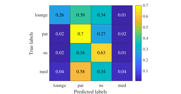
Fig. 2: Mean test confusion matrix (values are in fraction of samples) for TDNN-big with no foreground speaker detection.

5.1 Performance of the acoustic scene model

Table 1 shows the classification accuracy of all the models. First, we analyze the performance of different models on the FG active data. We note that the baseline DNN performs better ($6.39\%$ absolute improvement) than the majority guess classifier (Section 4.2), which confirms the existence of acoustic scene patterns in the audio data. Resnet-18 performs poorly for our task, possibly because of having too many trainable parameters with respect to the number of samples in the dataset (Section 4.3). TDNN-small and TDNN-big outperform the baseline DNN by an absolute $4.41\%$ and $3.16\%$ respectively.

Next we move our attention to the full dataset. Note that the number of samples is thrice of the FG active dataset. Resnet-18 still shows poor generalization. TDNN-small gets a little improvement over that baseline (absolute $\sim 1\%$). TDNN-big achieves an absolute boost of $4.12\%$ from the baseline DNN.

The results verify the efficacy of both the time delay networks to learn frame-level temporal dependencies even with fewer parameters compared to Resnet-18. TDNN-small has much fewer parameters than the baseline DNN, yet it outperforms the baseline for masked and unmasked cases. TDNN-big has similar number of parameters as the baseline, yet the former model shows better performance for both the data subsets.

The mean confusion matrix on test folds is shown in Figure 2 for the best model i.e., TDNN-big on the full dataset. It is evident that the model is more accurate in predicting nurse stations (‘ns’) and patient rooms (‘pat’), possibly because of having more training samples from these acoustic scenes. The performance of the model degrades in predicting the lounge, with almost equal number of confusing samples coming from nurse stations and patient rooms. The performance is poor for medication rooms (‘med’), possibly because of having the least number of training samples (see Section 4.2). Most of the confusions are originated from patient rooms, probably because of similar acoustic environment (comparatively quiet).

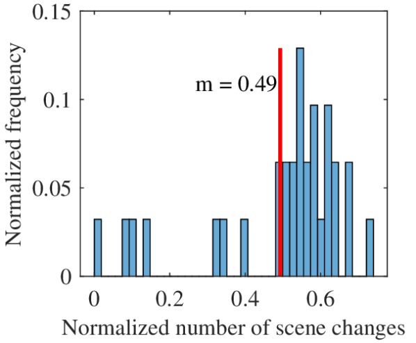
(a) Day shift, true sequence

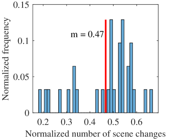
(b) Day shift, predicted sequence

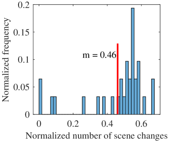
(c) Night shift, true sequence

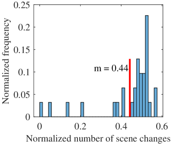
(d) Night shift, predicted sequence

Fig. 3: Histograms for normalized number of changes in true and predicted acoustic scene sequences for day and night shifts.

5.2 Characterizing predicted sequence of acoustic scenes

Here we try to explore if patterns in changes in acoustic scenes experienced by a certain participant is related to the nature of their job, specifically work shift and current position in the hospital. We first try to find pattern in the true acoustic scene sequences, and then, verify whether the predicted scene sequences provide similar patterns.

Continuing the formulation of Section 3.4, the histograms of normalized number of changes (see Equation 9) in the acoustic scene sequence (both for the true and the predicted sequences) are plotted in Figure 3 for day and night shift jobs. The mean values are annotated on the histograms with red bars. A quantitative analysis shows, for the true scene sequence, the mean of normalized number of changes ($1/{N_{\text{shift}}}\sum_{i=1}^{N_{\text{shift}}}\Delta\mathcal{Y}_{i}$ where $N_{\text{shift}}$ denotes number of participants in a particular shift) for day and night shifts are $0.49$ and $0.46$ respectively. Similar, decrease in mean can be observed with the same metric for predicted sequence, $\Delta\mathcal{\hat{Y}}_{i}$ as well: 0.47 and 0.44 respectively for day and night shifts.

This distinction is more prevalent when we do similar analysis on current job positions in the hospital: nursing vs. non-nursing. For true acoustic scene sequences, the mean of normalized number of changes are $0.25$ and $0.54$ for non-nursing and nursing jobs respectively. It also aligns with the intuition that the nursing jobs should be relatively more ambulatory. More interestingly, the same metric for the predicted scene sequences are $0.34$ and $0.49$, i.e., similar increasing trend for nursing jobs.

6 Conclusions and future directions

In this paper, we addressed the problem of predicting the acoustic scenes in a hospital workplace setting from long egocentric audio recordings. The audio recordings obtained using wearable close-talk microphones capture both participant’s speech and the ambient audio, and thus, it opens up new research directions in acoustic scene prediction through wearable or mobile devices.

We proposed a segment-level audio scene modeling to tackle extremely long audio recordings. We employed a time delay neural network to model the acoustic features at the segment level. The experiments showed that the employed time delay network performed the best in classifying the acoustic scenes, with or without an active foreground speaker detection step. Moreover, to characterize the egocentric view of acoustic scenes from the perspective of a participant, we explored the relationship between temporal pattern of the acoustic scenes experienced by the users with their job-types.

In the future, we will investigate how the egocentric acoustic patterns are related to individual mental states such as stress [29]. The proposed segment-level modeling is additionally attractive, since it helps compressing the data, and thus higher layers of temporal systems can be designed for end-to-end learning.

References

- [1] Dan Stowell, Dimitrios Giannoulis, Emmanouil Benetos, Mathieu Lagrange, and Mark D Plumbley, “Detection and classification of acoustic scenes and events,” IEEE Tran. on Multimedia, vol. 17, no. 10, pp. 1733–1746, 2015.
- [2] Jort F Gemmeke, Daniel PW Ellis, Dylan Freedman, Aren Jansen, Wade Lawrence, R Channing Moore, Manoj Plakal, and Marvin Ritter, “Audio set: An ontology and human-labeled dataset for audio events,” in ICASSP. IEEE, 2017, pp. 776–780.
- [3] Selina Chu, Shrikanth Narayanan, C-C Jay Kuo, and Maja J Mataric, “Where am i? scene recognition for mobile robots using audio features,” in Int. conference on multimedia and expo. IEEE, 2006, pp. 885–888.
- [4] Pradeep K Atrey, Namunu C Maddage, and Mohan S Kankanhalli, “Audio based event detection for multimedia surveillance,” in ICASSP. IEEE, 2006, vol. 5, pp. V–V.
- [5] Annamaria Mesaros, Toni Heittola, and Tuomas Virtanen, “A multi-device dataset for urban acoustic scene classification,” in Proceedings of the Det. and Classif. of Acoustic Scenes and Events 2018 Workshop, November 2018, pp. 9–13.
- [6] Annamaria Mesaros, Toni Heittola, Emmanouil Benetos, Peter Foster, Mathieu Lagrange, Tuomas Virtanen, and Mark D Plumbley, “Detection and classification of acoustic scenes and events: Outcome of the dcase 2016 challenge,” IEEE/ACM Tran. on Audio, Speech and Language Processing, vol. 26, no. 2, pp. 379–393, 2018.
- [7] Daniele Barchiesi, Dimitrios Giannoulis, Dan Stowell, and Mark D Plumbley, “Acoustic scene classification: Classifying environments from the sounds they produce,” IEEE Signal Processing Magazine, vol. 32, no. 3, pp. 16–34, 2015.
- [8] Annamaria Mesaros, Toni Heittola, and Tuomas Virtanen, “Tut database for acoustic scene classification and sound event detection,” in 2016 24th European Signal Processing Conference (EUSIPCO). IEEE, 2016, pp. 1128–1132.
- [9] Gaël Richard, Shiva Sundaram, and Shrikanth Narayanan, “An overview on perceptually motivated audio indexing and classification,” Proceedings of the IEEE, vol. 101, no. 9, pp. 1939–1954, 2013.
- [10] Antti J Eronen, Vesa T Peltonen, Juha T Tuomi, Anssi P Klapuri, Seppo Fagerlund, Timo Sorsa, Gaëtan Lorho, and Jyri Huopaniemi, “Audio-based context recognition,” IEEE Tran. on Audio, Speech, and Language Processing, vol. 14, no. 1, pp. 321–329, 2005.
- [11] Selina Chu, Shrikanth Narayanan, and C-C Jay Kuo, “Environmental sound recognition with time–frequency audio features,” IEEE Tran. on Audio, Speech, and Language Processing, vol. 17, no. 6, pp. 1142–1158, 2009.
- [12] A. Jati, N. Kumar, R. Chen, and P. Georgiou, “Hierarchy-aware loss function on a tree structured label space for audio event detection,” in ICASSP 2019 - 2019 IEEE International Conference on Acoustics, Speech and Signal Processing (ICASSP), May 2019, pp. 6–10.
- [13] Tiantian Feng, Amrutha Nadarajan, Colin Vaz, Brandon Booth, and Shrikanth Narayanan, “Tiles audio recorder: An unobtrusive wearable solution to track audio activity,” in 4th ACM Workshop on Wearable Sys. and Apps. ACM, 2018, pp. 33–38.
- [14] Reed Larson and Mihaly Csikszentmihalyi, “The experience sampling method,” in Flow and the foundations of positive psychology, pp. 21–34. Springer, 2014.
- [15] Vijayaditya Peddinti, Daniel Povey, and Sanjeev Khudanpur, “A time delay neural network architecture for efficient modeling of long temporal contexts,” in 16th Annual Conference of the International Speech Communication Association, 2015.
- [16] Arindam Jati, Paula G Williams, Brian Baucom, and Panayiotis Georgiou, “Towards predicting physiology from speech during stressful conversations: Heart rate and respiratory sinus arrhythmia,” in ICASSP. IEEE, 2018, pp. 4944–4948.
- [17] Brandon M Booth, Karel Mundnich, Tiantian Feng, Amrutha Nadarajan, Tiago H Falk, Jennifer L Villatte, Emilio Ferrara, and Shrikanth Narayanan, “Multimodal human and environmental sensing for longitudinal behavioral studies in naturalistic settings: Framework for sensor selection, deployment, and management,” Journal of medical Internet research, vol. 21, no. 8, pp. e12832, 2019.
- [18] Denise L Anthony, Ajit Appari, and M Eric Johnson, “Institutionalizing hipaa compliance: organizations and competing logics in us health care,” Journal of health and social behavior, vol. 55, no. 1, pp. 108–124, 2014.
- [19] Florian Eyben, Martin Wöllmer, and Björn Schuller, “Opensmile: the munich versatile and fast open-source audio feature extractor,” in Proceedings of the 18th ACM international conference on Multimedia. ACM, 2010, pp. 1459–1462.
- [20] Amrutha Nadarajan, Krishna Somandepalli, and Shrikanth S Narayanan, “Speaker agnostic foreground speech detection from audio recordings in workplace settings from wearable recorders,” in ICASSP. IEEE, 2019, pp. 6765–6769.
- [21] Karel Mundnich, Benjamin Girault, and Shrikanth Narayanan, “Bluetooth based indoor localization using triplet embeddings,” in ICASSP. IEEE, 2019, pp. 7570–7574.
- [22] Alex Waibel, Toshiyuki Hanazawa, Geoffrey Hinton, Kiyohiro Shikano, and Kevin J Lang, “Phoneme recognition using time-delay neural networks,” IEEE Tran. on acoustics, speech, and signal processing, vol. 37, no. 3, pp. 328–339, 1989.
- [23] David Snyder, Daniel Garcia-Romero, Gregory Sell, Daniel Povey, and Sanjeev Khudanpur, “X-vectors: Robust dnn embeddings for speaker recognition,” in ICASSP. IEEE, 2018, pp. 5329–5333.
- [24] Aaron van den Oord, Sander Dieleman, Heiga Zen, Karen Simonyan, Oriol Vinyals, Alex Graves, Nal Kalchbrenner, Andrew Senior, and Koray Kavukcuoglu, “Wavenet: A generative model for raw audio,” arXiv preprint arXiv:1609.03499, 2016.
- [25] Sergey Ioffe and Christian Szegedy, “Batch normalization: Accelerating deep network training by reducing internal covariate shift,” arXiv preprint arXiv:1502.03167, 2015.
- [26] Nitish Srivastava, Geoffrey Hinton, Alex Krizhevsky, Ilya Sutskever, and Ruslan Salakhutdinov, “Dropout: a simple way to prevent neural networks from overfitting,” JMLR, vol. 15, no. 1, pp. 1929–1958, 2014.
- [27] Kaiming He, Xiangyu Zhang, Shaoqing Ren, and Jian Sun, “Deep residual learning for image recognition,” in CVPR. IEEE, 2016, pp. 770–778.
- [28] Diederik P Kingma and Jimmy Ba, “Adam: A method for stochastic optimization,” preprint arXiv:1412.6980, 2014.
- [29] Michelle L’Hommedieu, Justin H. L’Hommedieu, Cynthia Begay, Alison Schenone, Lida Dimitropoulou, Gayla Margolin, Tiago H. Falk, Emilio Ferrara, Kristina Lerman, and Shrikanth Narayanan, “Lessons learned: Recommendations for implementing a longitudinal study using wearable and environmental sensors in a healthcare organization,” Journal of medical Internet research (JMIR), mHealth and uHealth, 2019.