The hydroxyl satellite-line ‘flip’ as a tracer of expanding Hii regions

Abstract

Observations of the four ${}^{2}\Pi_{3/2},~{}J=3/2$ ground state transitions of the hydroxyl radical (OH) have emerged as an informative tracer of molecular gas in the Galactic ISM. We discuss an OH spectral feature known as the ‘flip’, in which the satellite lines at 1612 and 1720 MHz flip – one from emission to absorption and the other the reverse – across a closely blended double feature. We highlight 30 examples of the flip from the literature, 27 of which exhibit the same orientation with respect to velocity: the 1720 MHz line is seen in emission at more negative velocities. These same examples are also observed toward bright background continuum, many (perhaps all) show stimulated emission, and 23 of these are coincident in on-sky position and velocity with Hii radio recombination lines. To explain these remarkable correlations we propose that the 1720 MHz stimulated emission originates in heated and compressed post-shock gas expanding away from a central Hii region, which collides with cooler and more diffuse gas hosting the 1612 MHz stimulated emission. The foreground gas dominates the spectrum due to the bright central continuum, hence the expanding post-shock gas is blue-shifted relative to the stationary pre-shock gas. We employ non-LTE excitation modelling to examine this scenario, and find that indeed FIR emission from warm dust adjacent to the Hii region radiatively pumps the 1612 MHz line in the diffuse, cool gas ahead of the expanding shock front, while collisional pumping in the warm, dense shocked gas inverts the 1720 MHz line.

1 Introduction

The hydroxyl radical, OH, is a sensitive tracer of the physical characteristics and dynamics of the molecular interstellar medium (ISM). OH was the first molecule discovered in the ISM (Weinreb et al., 1963) and though its ground rotational state hyperfine transitions are weak, many early works used it to study the distribution and properties of Galactic molecular gas (Barrett, 1964; Robinson & McGee, 1967; Rogers & Barrett, 1967; Goss, 1968; Heiles, 1968, 1969; Turner, 1979). However, once the technology was developed to observe the much brighter rotational transitions of carbon monoxide – particularly the CO ($J=1\rightarrow 0$) transition (e.g. Wilson et al., 1970; Solomon et al., 1972) – the focus of OH observations moved away from its ability to trace the molecular ISM as a whole, and more towards its ability to trace specific excitation conditions (Elitzur, 1976; Elitzur et al., 1976; Guibert et al., 1978; Elitzur, 1978), such as those responsible for masing in each of the four ground-rotational state transitions.

Though CO remains a very effective tracer of molecular gas in the ISM, a significant amount of molecular gas in more diffuse regions is not traced well by CO (e.g. Reach et al., 1994; Grenier et al., 2005; Planck Collaboration et al., 2011; Remy et al., 2018), but is expected to be well-traced by OH (Wannier et al., 1993; Liszt & Lucas, 1996; Barriault et al., 2010; Allen et al., 2012; Allen et al., 2015; Li et al., 2018). This has led to a resurgence of interest in the observation and interpretation of OH as a supplementary tracer of molecular gas (e.g. Dawson et al., 2014; Rugel et al., 2018; Nguyen et al., 2018; Engelke & Allen, 2019).

The four ${}^{2}\Pi_{3/2},~{}J=3/2$  ground state transitions of OH occur at 1612.231, 1665.402, 1667.359 and 1720.530 MHz. These transitions are generally weak, and therefore are most readily observed in absorption against bright background continuum emission. OH in the molecular ISM is almost never in local thermodynamic equilibrium (LTE), so the excitation temperatures $T_{\rm ex}$ of its transitions are not a reliable indication of the kinetic temperature of the gas $T_{\rm gas}$ (Elitzur, 1992). Without the ability to assume LTE, the interpretation of OH emission and absorption can be quite difficult. Thus when considering the molecular ISM, many studies focus on the stronger ‘main’ lines at 1665 and 1667 MHz as their excitation temperatures – though often sub-thermal – tend to not deviate from LTE as strongly as the satellite lines under a wide range of local conditions (e.g. Baud & Wouterloot, 1980; Barriault et al., 2010; Nguyen et al., 2018; Li et al., 2018). In such cases reasonable assumptions may be applied to the excitation of the main lines and properties of the gas can be inferred without solving for the population of the four levels within the OH ground rotational state (e.g. Barriault et al., 2010; Rugel et al., 2018).

However, the complexity of OH satellite-line excitation is sometimes an advantage, as its greater sensitivity to local environmental conditions carries information that may not be captured by the main lines. For example, stimulated emission of the OH satellite lines (i.e. when $T_{\rm ex}<0$) has been studied extensively in the context of OH masers (e.g. Elitzur, 1976; Elitzur et al., 1976; Guibert et al., 1978; Pavlakis & Kylafis, 1996). Stimulated emission in the 1612 MHz line is generally interpreted as indicating a radiatively-dominated environment, while stimulated emission in the 1720 MHz line is interpreted as indicating a collisionally-dominated environment (Elitzur, 1992). High-gain 1612 MHz masers (i.e. where optical depth $|\tau|\gg 1$) trace both active star formation (Caswell, 1999) and evolved stellar sources such as OH-IR stars (Elitzur et al., 1976). High-gain 1720 MHz masers trace the shocked gas of supernova remnants (Frail et al., 1994; Frail et al., 1996). Widespread weak satellite-line maser emission (i.e. where $|\tau|<1$) is also observed in the Milky Way (e.g. Turner, 1982; Dawson et al., 2014; Walsh et al., 2016; Rugel et al., 2018).

Here we present an example of a peculiar OH profile shape sometimes known as the satellite-line ‘flip’ – first described by Caswell & Haynes (1975), with the first examples seen in the literature almost a decade earlier (Goss, 1967). A typical example of the profile is given in Fig. 1. On one side of the feature the 1612 MHz line is seen in absorption while the 1720 MHz line is in emission. The lines then flip their relative orientation to have the 1612 MHz line in emission and the 1720 MHz line in absorption, all within a closely blended double feature. Meanwhile, both main lines are in absorption, often obscuring the fact that two velocity components exist.

van Langevelde et al. (1995) carried out non-LTE excitation calculations in the context of an extragalactic example of the flip towards the nucleus of Cen A (G200.63-42.76). They tested a range of number densities, column densities, gas temperatures and radiation fields with an assumed velocity dispersion of $\Delta V=1\,$km s^-1, and found that in models where a flip could be achieved, it occurred where two gas components lay on either side of $N_{\rm OH}/\Delta V\approx 10^{15}\,$cm^-2 km^-1 s, in broad agreement with Elitzur (1976). They therefore interpret the flip as indicating $N_{\rm OH}/\Delta V\approx 10^{15}\,$cm^-2 km^-1 s. Other than this work and those that apply its conclusions (e.g. Frayer et al., 1998; Rugel et al., 2018), no local astrophysical process has been proposed to account for the flip. In Section 3 we outline our own non-LTE excitation modelling and find that the effects of line overlap complicate the picture reported by van Langevelde et al. (1995).

In this work we identify, from our own observations and from the literature, 30 examples of the satellite-line flip (Goss, 1967; Caswell & Robinson, 1974; Caswell & Haynes, 1975; Turner, 1979; van Langevelde et al., 1995; Frayer et al., 1998; Brooks & Whiteoak, 2001; Dawson et al., 2014; Rugel et al., 2018; Ogbodo et al., 2020) presented in Table 1. All but two extragalactic examples (towards G200.63-42.76 (van Langevelde et al., 1995) and towards G277.81+32.42 (Frayer et al., 1998)) are within our Galaxy. With only three exceptions, all of these examples are observations of OH gas towards bright background continuum sources, most of which may be interpreted as locally associated Hii regions. The bright background continuum suggests that the observed emission is stimulated emission (i.e. indicating a population inversion where optical depth $\tau<0$ and $T_{\rm ex}<0$), as opposed to thermal emission (i.e. where $\tau>0$ and $T_{\rm ex}>T_{\rm c}$).

We note the hitherto unnoticed fact that all of the flips observed towards bright background continuum sources (27/30) exhibit the same orientation in velocity: the 1720 MHz inversion is seen at more negative velocities and the 1612 MHz inversion at more positive velocities. This remarkable trend leads us to propose a physical explanation of the flip where the 1612 MHz and 1720 MHz inversions originate in pre- and post-shock gas (respectively) surrounding an Hii region. To justify this model we first outline the key factors affecting OH excitation in the context of the satellite-line flip in Section 2. We outline our physical model in detail in Section 3, discuss its implications and limitations in Section 4 and present our conclusions in Section 5.

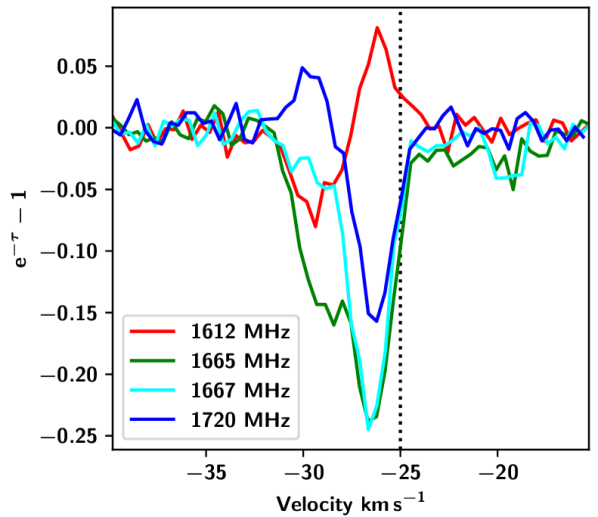
Figure 1: Optical depth observations of hydroxyl made with the Australia Telescope Compact Array towards the bright background continuum source G340.79-1.02 from Petzler et al. (2020, in prep.) as an illustrative example of the OH satellite-line flip. The 1612 MHz line can be seen in absorption at more negative velocities, transitioning to stimulated emission at -28 km s^-1. The 1720 MHz line shows the opposite behaviour with stimulated emission at more negative velocities, transitioning to absorption at -28 km s^-1. Both main lines (1665 and 1667 MHz) are in absorption but clearly indicate the presence of two blended velocity components, with peaks roughly corresponding to the peak emission in each satellite line. A radio-recombination line is detected toward this source, centred at -25 km s^-1 (dotted line), indicating the presence of an Hii region.

$l\,^{\circ}$	$b\,^{\circ\;a}$	$v$ (km s-1)$\,{}^{b}$		1612 MHz		1720 MHz		Unitsc	$\theta_{1/2}\,^{d}$	Hii Assoc.e	Ref.f
		Blue	Red	Blue	Red	Blue	Red		arcmin	Y/N
8.10	0.20	13	17.8	-0.15	0.11	0.25	-0.37	K	18.8	Y	A
12.80	-0.20	32.5	38.5	-0.2	0.4	0.64	-0.3	Jy	0.12$\dagger$	Y	B
14.00	-0.60	17.8	22.9	-0.25	0.13	0.14	-0.22	K	18.8	Y	A
19.08	-0.29	62	71	-10	10	10	-15	K∗	0.77$\dagger$	Y	C
19.61	-0.23	43.9	48.2	-0.32	0.1	0.56	-0.15	Jy	0.12$\dagger$	Y	B
30.50	0.00	90	95.2	-0.52	0.34	0.18	-0.34	K	18.8	Y	A
30.78	-0.14	90	95	-1	0.3	0.6	-0.9	K	33.4	Y	D
32.80	0.19	7	20	-15	15	70	-60	K∗	0.77$\dagger$	Y	C
35.20	-1.70	39.8	43.9	-0.18	0.19	0.28	-0.36	K	18.8	Y	A
48.92	-0.28	5.6	6.5	-0.165	0.029	0.127	-0.104	$e^{-\tau}-1$	0.5	N	E
49.37	-0.30	63	66	-90	100	90	-80	K∗	0.77$\dagger$	Y	C
133.70	1.20	-40.6	-38	-1	0.4	3.06	-0.44	K	18.8	Y	A
172.80	-13.24	5.3	6.8	0.2	-0.033	-0.067	0.067	K	3	N	F
173.40	-13.26	5	8	0.133	-0.04	-0.023	0.057	K	8.2	N	G
175.83	-9.36	7.1	7.8	0.003	-0.017	-0.043	0.031	$e^{-\tau}-1$	0.5	N	E
200.63	-42.76	550	555	-0.11	0.1	0.13	-0.1	Jy	0.11$\dagger$	Y	H
267.90	-1.10	0.1	2.1	-1.1	1	0.9	-4.9	K	12	Y	I
277.81	32.42	200	240	-0.015	0.01	0.015	-0.007	Jy	0.02$\dagger$	Y	J
316.80	0.00	-38	-35	-2.5	1.9	1.9	-1.9	K	12.6	Y	K
332.71	-0.71	-52	-48	-6	5	1	-9	K	2.5	Y	L
333.09	-0.50	-56	-51	-10	5	5	-7	K	2.5	Y	L
333.09	-0.50	-43	-39	-3	2	3	-3	K	2.5	Y	L
336.95	-0.20	-83	-75	-0.25	0.25	0.25	-0.3	K	12.6	Y	M
336.95	-0.20	-43	-38	-0.5	0.5	0.25	-0.75	K	12.6	N	M
337.10	-0.20	-44	-36.4	-0.3	0.4	0.1	-0.54	K	18.8	Y	A
337.80	-0.10	-53	-36.2	-0.3	0.53	0.23	-0.6	K	18.8	Y	A
340.79	-1.02	-29.2	-26.5	-0.07	0.081	0.038	-0.148	$e^{-\tau}-1$	0.5$\dagger$	Y	N
342.00	-0.20	-33	-23	-0.4	0.1	0.2	-0.2	K	12.6	Y	M
351.42	0.66	-6.1	-1	-0.28	0.1	0.19	-0.18	$e^{-\tau}-1$	0.37$\dagger$	Y	O
353.41	-0.30	-18.3	-15.2	-0.063	0.081	0.166	-0.125	$e^{-\tau}-1$	0.5$\dagger$	Y	N

Table 1: Spectra exhibiting the satellite-line flip: where the conjugate relationship between the satellite lines flips across a closely-blended double feature. ^aLocations of each flip are given in Galactic coordinates. ^bThe velocities of the more blue-shifted component and the more red-shifted component are given along with the peak values measured at 1612 and 1720 MHz. As these examples are drawn from disparate publications, the values of these peaks are approximate. ^c Units of measurement are either: continuum subtracted brightness temperature (K, ^∗converted from Jy beam^-1), continuum subtracted flux density (Jy), or optical depth ($e^{-\tau}-1$). In all cases a positive value indicates relative emission and a negative value indicates relative absorption. ^dThe resolution of the flip observation is given in arcmin, and $\dagger$ indicates interferometric observations. ^eThe presence or absence of an associated Hii region is indicated. ^fReferences: (A) Turner (1979), (B) Ogbodo et al. (2020), (C) Rugel et al. (2018), (D) Goss (1967), (E) Petzler et al. (2020 in prep), (F) Xu et al. (2016), (G) Ebisawa et al. (2019), (H) van Langevelde et al. (1995), (I) Manchester et al. (1970), (J) Frayer et al. (1998), (K) Caswell & Robinson (1974), (L) Cunningham M.R. (private communication), (M) Dawson et al. (2014), (N) Petzler et al. (2020 in prep), (O) Brooks & Whiteoak (2001).

2 OH satellite-line excitation

In this section we outline the level population requirements for satellite-line inversion as seen in the satellite-line flip, and the de-excitation pathways that lead to these populations (Elitzur, 1976; Elitzur et al., 1976; Guibert et al., 1978). We then discuss the environmental conditions that influence the relative dominance of these de-excitation pathways, and how these could manifest in the observed satellite-line flip. An exhaustive discussion of this subject can be found in Elitzur (1992).

The OH ${}^{2}\Pi_{3/2},~{}J=3/2$  ground rotational state is split into four levels via $\Lambda$-doubling and hyperfine splitting. These levels, as well as their allowed transitions at 1612, 1665, 1667 and 1720 MHz, are illustrated in Fig. 2. Due to the different degeneracies of its upper and lower levels, inversion in the 1612 MHz line is achieved when the population of its upper level is greater than $3/5$ that of its lower level. Inversion of the 1720 MHz line is achieved when the population of its upper level is greater than $5/3$ that of its lower level (Elitzur, 1992).

The relative population of the OH ground state hyperfine levels in the ISM is largely determined by cascade pathways into the ground state from previously-excited higher rotational states. As all cascades into the ground state will pass through the first excited ${}^{2}\Pi_{3/2},~{}J=5/2$ or the second excited ${}^{2}\Pi_{1/2},~{}J=1/2$ rotational states (Elitzur, 1992), only these are illustrated in Fig. 3. Also illustrated in Fig. 3 are the allowed transitions (determined by quantum mechanical selection rules) from the levels within those excited rotational states into the levels of the ground state. If the radiative decay pathways from the first and second excited rotational states into the ground state are optically thick, then the rates of individual transitions within each pathway are independent of line strength due to photon trapping, and depend only on the number of possible transitions into the ground state (Elitzur, 1976).

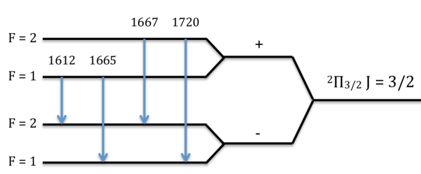
Figure 2: Energy level diagram of the ${}^{2}\Pi_{3/2},~{}J=3/2$ ground state of hydroxyl. The ground state is split into four levels due to $\Lambda$-doubling and hyperfine splitting, with 4 allowed transitions between these levels: ‘main’ lines at 1665.402 and 1667.359 MHz, and ‘satellite’ lines at 1612.231 and 1720.530 MHz. The degeneracies of the levels are given by $g=2F+1$.

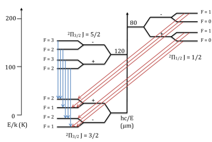
Figure 3: Schematic of the three lowest rotational states of OH, as well as the $\Lambda$ and hyperfine splitting of those states. Excitations above the ${}^{2}\Pi_{3/2},~{}J=3/2$ ground state will cascade back down to it via the ${}^{2}\Pi_{3/2},~{}J=5/2$ state, or the ${}^{2}\Pi_{1/2},~{}J=1/2$ state. Allowable transitions are those where parity is changed and $|\Delta F|$ = 1, 0; shown in blue at left and red on the schematic. The energy scale is given at left in kelvin, and the wavelengths of the IR transitions are shown at centre in $\mu$m. The splittings of the $\Lambda$ and hyperfine levels are greatly exaggerated for clarity.

As illustrated in Fig. 2, the main-line transitions at 1665 and 1667 MHz occur between upper and lower levels with the same total angular momentum quantum number $F$, while the satellite-line transitions occur between levels with different $F$ number. The $F$ numbers of the different levels of the ground and excited rotational states (see Fig. 3) introduce an asymmetry in the possible transitions into the ground state for the satellite lines but not for the main lines: there are more allowed transitions from the first excited ${}^{2}\Pi_{3/2},~{}J=5/2$ state into the upper level of the 1720 MHz transition than there are into its lower level. Similarly, there are more allowed transitions from the second excited ${}^{2}\Pi_{1/2},~{}J=1/2$ state into the upper level of the 1612 MHz transition than there are into its lower level. Environmental factors that preference the cascade pathway from one of the excited rotational states over the other can therefore provide a pumping mechanism that inverts the 1720 or 1612 MHz transitions. In general, when one of the satellite-lines is inverted in this manner, the other satellite-line is sub-thermally excited, leading to the ‘conjugate’ behaviour often observed in the satellite lines (e.g. van Langevelde et al., 1995; Ebisawa et al., 2019), the ‘flip’ being one manifestation of this behaviour.

There are three main physical mechanisms by which one of these pathways is preferred and hence one of the satellite lines can be inverted:

1. In radiatively-dominated environments where a wide range of photon energies are available (i.e. far-infrared emission from warm dust), and where the transitions into the ground state from both the first and second excited rotational levels are optically thick, the two cascade pathways are equally likely, and the populations of each of the levels of the ground state will be roughly equal. Due to the level degeneracies (3 and 5 for the upper and lower levels of the 1612 MHz transition, respectively, and the reverse for the 1720 MHz transition) this leads to sub-thermal excitation of the 1720 MHz line and inversion of the 1612 MHz line (Elitzur et al., 1976).

2. In collisionally-dominated environments where the transitions into the ground state from both the first and second excited rotational levels are optically thick, high temperatures can invert the 1612 MHz line and lower temperatures can invert the 1720 MHz line (Elitzur, 1976). Lower temperatures lead to a sufficient reduction in excitation into higher rotational states that the pathway via the ${}^{2}\Pi_{3/2},~{}J=5/2$ state is left to dominate the population of the ground state levels. This pathway will in effect transfer molecules from the $F=1$ levels of the ground state to the $F=2$ levels, leading to sub-thermal excitation in the 1612 MHz line and inversion of the 1720 MHz line.

3. In cases where the 1612 MHz pumping mechanism is active, it can be deactivated by lowering the OH column, which can then allow the 1720 MHz line to invert. The line strengths for transitions to the ground state from the second excited rotational state are about an order of magnitude lower than those from the first excited rotational state. As a consequence, for a given velocity dispersion there exists a range of column densities for which transitions from the second excited (${}^{2}\Pi_{1/2},~{}J=1/2$) rotational level are optically thin while transitions from the first excited (${}^{2}\Pi_{3/2},~{}J=5/2$) level are optically thick. van Langevelde et al. (1995) found that this range is $N_{\rm OH}/\Delta V\approx 1$–$9\times 10^{14}$ cm^-2 km^-1 s. In this case, the rate of transitions from the second excited state to the ground state will be determined by their individual line strengths, which will tend to maintain the original population of the ground state levels. This prevents the transfer of molecules from the $F=2$ levels of the ground state to the $F=1$ levels, thus disabling the 1612 MHz pumping mechanism (Elitzur, 1976).

In the context of the flip towards the nucleus of Cen A (G200.63-42.76), van Langevelde et al. (1995) performed non-LTE calculations of OH assuming $\Delta V=1$ km s^-1. Their models included a radiation field characterised by two IR components: one with dust temperature $T_{\rm dust}=43\,$K and external visual extinction $A_{\mathrm{v}}({\rm ext})$ $=30\,$mag, and the other with $T_{\rm dust}=150\,$K and $A_{\mathrm{v}}({\rm ext})$ $=3\,$mag. This choice was motivated by the excess 25 and 12 ${\rm\mu m}$ emission observed along the disk of Cen A by Marston & Dickens (1988). These mid-IR components allowed for excitation into the ${}^{2}\Pi_{1/2}~{}J=5/2$ rotational state – the highest state included in their modelling – through absorption of the 35 ${\rm\mu m}$ line. These OH molecules then cascade down to the ground rotational state via the second excited rotational state, allowing the inversion of the 1612 MHz line. They found that this 1612 MHz inversion could then be disabled and the 1720 MHz line inverted when $N_{\rm OH}/\Delta V\approx 10^{15}\,$cm^-2 km^-1 s.

As we discuss in the following section, we also find that the flip can be produced by changes in $N_{\rm OH}/\Delta V$ in radiatively dominated environments, but due to line overlap this trend is only seen while $\Delta V\lesssim 1$ km s^-1. Instead we find that a flip can also be generated by a change in a combination of parameters such as gas temperature and number density, and that these changes can naturally exist in the environment around an expanding Hii region.

3 Physical explanation of the flip

We propose that the satellite-line flip is best explained by a physical model where two parcels of gas exist on either side of a shock expanding away from a central Hii region, as illustrated by the cartoon in Fig. 4. The Hii region provides the radiation required to invert the 1612 MHz line in the surrounding ambient molecular cloud, while the increased gas temperature and number density in the post-shock gas disable the 1612 MHz inversion and invert the 1720 MHz line. The central Hii region then provides the bright background continuum which leads the foreground emission and absorption to dominate the observed brightness temperature, thus accounting for the striking velocity bias seen in examples of the satellite-line flip. Our reasoning and evidence are detailed in this section.

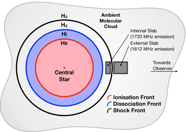
Figure 4: Cartoon of an expanding Hii region and associated fronts. The relative positions of the ionisation front (red), the dissociation front (blue) and the shock front (black) expanding from the central star into an ambient molecular medium are shown. The locations of parallel slabs internal (post-shock) and external (pre-shock) to the shock front modelled in Fig. 6 are indicated. The widths of the Hi and post-shock H₂ regions are exaggerated for clarity.

The flip is most commonly observed with the 1720 MHz line inverted at more negative velocities and the 1612 MHz line inverted at more positive velocities – 90% (27/30) of the examples shown in Table 1 show this orientation. The separation in velocity suggests that the satellite line flip may be associated with a coherent velocity field, such as expansion and/or infall. The observation that most of the flips have the 1720 MHz inversion at more negative velocities implies a bias in the orientation of this velocity field with respect to the observer. As examples of the flip are observed in all quadrants of the Milky Way, this bias is not due to the large-scale Galactic velocity field. Instead, we note that all of the flips that demonstrate this velocity bias are also observed against bright background continuum (27/30). When the continuum brightness temperature $T_{\rm c}\gg|T_{\rm ex}|$, absorption or stimulated emission from the foreground gas will dominate the observed line brightness temperature. Therefore, if the source of background continuum was also the source of the velocity field, this could provide a natural explanation for the observed bias in the orientation of the flip – in principle, a physically-associated source of continuum (e.g. an embedded Hii region) could provide the necessary bright background continuum and drive expansion.

This led us to consider whether there was evidence for a local association between the OH gas and the background continuum illuminating it: i.e. whether the continuum source could be identified as an Hii region and localised in on-sky position and velocity to the observed flip.

All but one of the examples of the flip towards bright background continuum (26/27) coincide positionally on the sky with the location of a known Hii region. A flip was considered to ‘coincide’ with an Hii region if the half-power beam-width with which it was observed overlapped with the recorded radius of an Hii region. In the case of the two extragalactic examples, specific Hii regions are not resolved but both are associated with large molecular structures that contain Hii regions (Hodge & Kennicutt, 1983; Ulvestad & Antonucci, 1991). Excluding these two extragalactic examples, all but one of the flips associated on the sky with specific Hii regions (23/24) also have recorded radio recombination lines (RRL) within $\pm 10$ km s^-1 of one or other component of the flip. The relative velocities of the components of the flips with the RRL of on-sky overlapping Hii regions are illustrated in Fig. 5. All Hii data were obtained from the Wide-field Infrared Survey Explorer (WISE Anderson et al., 2014, 2015; Anderson et al., 2018) and from the Southern Hii Region Discovery Survey (SHRDS Wenger et al., 2019). Any more precise association with individual Hii regions was not possible given the large full width at half-maximum of radio recombination lines (WISE median $\Delta V=25$ km s^-1) compared to the average separation of the flips, and velocity blending along the line of sight.

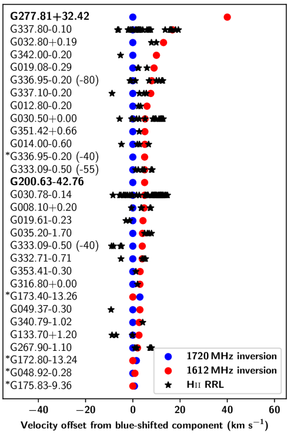
Figure 5: Velocity separation of the 1720 MHz emission (blue circles) and 1612 MHz emission (red circles) components of the examples of the satellite-line flip given in Table 1. The velocities of RRL for Hii regions overlapping in on-sky position with each example of the flip are indicated by black stars. Extragalactic examples of the flip are highlighted with boldface type, and those without associated Hii RRL are indicated with an asterisk (^∗). Details of how these associations were determined are given in the text. All velocities are plotted as offsets from the blue-shifted component of the flip. The flips are plotted in descending order of the velocity offset of their red-shifted component to illustrate the distribution of velocity separation. All Hii data were obtained from the Wide-field Infrared Survey Explorer (WISE Anderson et al., 2014, 2015; Anderson et al., 2018) and from the Southern Hii Region Discovery Survey (SHRDS Wenger et al., 2019).

We then undertook non-LTE molecular excitation modelling to determine if the conditions expected in the molecular gas surrounding an Hii region could give rise to the flip. Our modelling explored ‘reasonable’ values of gas temperature ($T_{\rm gas}=5$–$150$ K), number density ($n_{\rm H_{2}}=1$–$10^{6}\,{\rm cm}^{-3}$), velocity dispersion ($\Delta V=0.5$–$10$ km s^-1), column density ($N_{\rm OH}=10^{12}$–$10^{18}\,{\rm cm}^{-2}$), internal and external dust temperatures ($T_{\rm dust}\textrm{(int)}=10$–$50\,$K and $T_{\rm dust}\textrm{(ext)}=10$–$100\,$K, respectively) and external visual extinction ($A_{\mathrm{v}}({\rm ext})$ $=0.1$–$10\,$mag). The range of parameters tested were chosen to be consistent with expected conditions in the molecular ISM and the previous findings of Elitzur et al. (1976) and van Langevelde et al. (1995). It was also informed by 1D hydrodynamical modelling of the shock, dissociation and ionisation fronts surrounding an expanding Hii region (Hosokawa & Inutsuka, 2005, 2006), as well as modelling and observations of dust temperatures around Hii regions (Churchwell et al., 1990; Okumura et al., 1996; Anderson et al., 2012; Deharveng et al., 2012).

Hosokawa & Inutsuka (2006) modelled the expansion of an Hii region surrounding solitary O-type stars in a typical host molecular cloud with $n_{\rm H_{2}}=10^{3}\,{\rm cm}^{-3}$. Their models showed the velocity discontinuity at the shock to be $\approx 1-8$ km s^-1, consistent with a large portion of the flips identified in Table 1. They also found that the post-shock gas could be heated to a gas temperature 50–100 K warmer than the pre-shock gas, and that the number density of the post-shock gas was increased by a factor of 10.

Observations consistently find that dust temperatures in molecular clouds are typically 10–30 K (Okumura et al., 1996; Anderson et al., 2012; Deharveng et al., 2012), and only rarely exceed 40 K (Dupac et al., 2003; Salgado et al., 2016). We therefore considered internal dust temperatures $T_{\rm dust}(\rm{int})=10$–$50\,$K. Modelling predicts, however, that the hottest dust surrounding an Hii region (i.e. within the photodissociation zone) could be up to several $10^{2}\,$K – but only around the youngest stars and in a very thin layer (Wolfire & Churchwell, 1994). We therefore considered external dust temperatures $T_{\rm dust}(\rm{ext})=10$–$100$ K and visual extinction $A_{\mathrm{v}}({\rm ext})$ $=0.1$–$10$ mag, but models with high $T_{\rm dust}(\rm{ext})$ were paired with low $A_{\mathrm{v}}({\rm ext})$ and vice versa.

The full parameter ranges tested are outlined in Table 2, and extend from quiescent, diffuse molecular gas to shock-compressed gas nearing dissociation in close proximity to an Hii region. Values outside these ranges that were also tested are referred to explicitly in Section 4.

property	values explored
$N_{\rm OH}$	$10^{12}$	$-~{}10^{18}\,{\rm cm^{-2}}$
$\Delta V$	$0.5$	$-~{}10\,$km s-1
$T_{\rm gas}$	$5$	$-~{}150\,{\rm K}$
$n_{\rm H_{2}}$	$10^{0}$	$-~{}10^{6}\,{\rm cm^{-3}}$
$T_{\rm dust}$ (internal)	$10$	$-~{}50\,{\rm K}$
$T_{\rm dust}$ (external)	$10$	$-~{}100\,{\rm K}$
$A_{\rm v}$ (external)	$0.1$	$-~{}10\,{\rm mag}$

Table 2: Properties of models explored using our molecular excitation code to approximate slabs of molecular gas surrounding an Hii region as illustrated in Fig. 4. The effects of gas temperature, velocity dispersion, OH column density, H₂ number density, internal dust temperature and radiation field as defined by external dust temperature and visual extinction on the satellite-line flip were explored across the region of parameter space indicated by the ranges given. Values of ortho : total H₂ ratio (0.75), OH and He abundances relative to H₂ ($10^{-7}$ and $10^{-4}$, respectively) were kept constant. The resulting optical depths at 1612 and 1720 MHz found from this modelling are illustrated in Fig. 6.

Our non-LTE molecular excitation code was used to determine the level populations of the lowest 8 rotational states of OH and their hyperfine levels (32 levels in all). The code employed an escape probability approach to radiative transfer in a uniform slab including line overlap, following the treatment of Lockett & Elitzur (1989). Line overlap occurs when the Doppler shift due to the velocity dispersion in the gas spans the difference in frequency between the 3 or 4 IR transitions linking the same pair of rungs of the OH rotational ladder. The most relevant IR transitions are those between the first two excited rotational states and the ground rotational state (i.e. those illustrated in Fig. 3). Line overlap disrupts the population inversions caused by the pumping mechanisms outlined in Section 2 by allowing photons emitted in one IR transition to be reabsorbed in a neighbouring IR transition when the linewidths exceed $\sim 1$ km s^-1. The escape probability approach makes the approximation that the OH level population does not vary with depth within the slab. The level population is solved iteratively for consistency with the rates of collisional excitation and de-excitation, spontaneous emission, and of absorption and stimulated emission implied by the mean intensity of the radiation field within the slab. The mean intensity (frequency-dependent but averaged over solid angle and position) includes the source function and absorption coefficient implied by the level population, as well as thermal emission from external and internal dust.

The energy levels and Einstein $A$ coefficients for the hyperfine transitions within rotational states were taken from Destombes et al. (1977), while the infrared transitions and $A$ coefficients were taken from Brown et al. (1982). Collisional rate coefficients with H₂ were taken from Offer et al. (1994) for transitions between the lowest 6 rotational levels, with hard sphere collision rates used for transitions involving the upper two rotational levels. Collisional rate coefficients with helium were taken from Kłos et al. (2007) and were computed for electrons using the prescription from Chu (1976). The infrared radiation fields from dust lying outside the slab and within the slab were represented by grey body models using the MRN dust extinction curve of Draine & Lee (1984). The input parameters were gas temperature $T_{\rm gas}$, velocity FWHM $\Delta V$ of the Gaussian line profile (which implicitly includes the contributions of thermal and “microturbulent” broadening), fraction of ortho-H₂, abundances of OH, He and electrons relative to H₂ ($X_{\rm OH}$, $X_{\rm He}$, $X_{\rm e}$), external dust temperature $T_{\rm dust}({\rm ext})$ and external visual extinction $A_{\mathrm{v}}({\rm ext})$, internal dust temperature $T_{\rm dust}({\rm int})$, number density $n_{\rm H_{2}}$ and column density $N_{\rm OH}$. The extinction of the dust internal to the slab is computed using $A_{\mathrm{v}}\mathrm{(int)}=N_{\rm OH}/X_{\rm OH}/(10^{21}\mathrm{cm^{-2}})$. The electron abundance relative to H₂ ($X_{\rm e}$) declined with increasing $n_{\rm H_{2}}$, ranging from $X_{\rm e}=10^{-4}$ when $n_{\rm H_{2}}=10^{2}\,{\rm cm^{-3}}$ to $X_{\rm e}=10^{-7.5}$ when $n_{\rm H_{2}}=10^{5}\,{\rm cm^{-3}}$, reflecting the relative dominance of photo- and cosmic ray ionisation expected in these regimes. The fraction of ortho-H₂ (0.75), $X_{\rm OH}$ ($n_{\rm OH}/n_{\rm H_{2}}=10^{-7}$) and $X_{\rm He}$ ($n_{\rm He}/n_{\rm H_{2}}=0.2$) were held constant for all models. Some key results of our modelling are illustrated in Fig. 6.

‘Low’ Radiation: $T_{\rm dust}({\rm int})=20$ K $T_{\rm dust}({\rm ext})=20$ K $A_{\mathrm{v}}({\rm ext})$ $=0.3$ mag
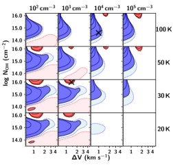
‘High’ Radiation: $T_{\rm dust}({\rm int})=20$ K $T_{\rm dust}({\rm ext})=70$ K $A_{\mathrm{v}}({\rm ext})$ $=0.1$ mag

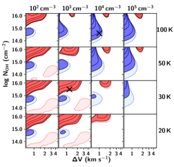
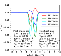
Figure 6: Left panels: Regions of ${\rm log}\,N_{\rm OH}$ vs $\Delta V$ parameter space where the 1612 MHz (pink) and 1720 MHz (blue) OH satellite lines are inverted. Dotted contours and lighter shading indicate where $-0.02\leq\tau\leq 0$. Solid contours and darker shading represent areas of ‘significant’ inversion where $\tau=-(0.02,0.1,0.5,1,2,3,4)$. The grids both have constant internal dust temperature $T_{\rm dust}(\rm int)=20$ K. From top to bottom the grids increase in external dust temperature $T_{\rm dust}(\rm ext)=20-70$ K and decrease in visual extinction (equivalent to the thickness of the external dust layer) $A_{\mathrm{v}}({\rm ext})$ $=0.3-0.1$ mag. The grids therefore represent a transition from ‘low’ radiation at the top to ‘high’ radiation at the bottom. These parameters were chosen to represent increasing proximity to the central ionising sources and/or differences in the properties of those sources and their surrounding ISM. The panels in each row of the grids correspond to gas temperature $T_{\rm gas}=20,~{}30,~{}50,~{}100\,{\rm K}$ from bottom to top; the columns to number density $n_{\rm H_{2}}=10^{2},~{}10^{3},~{}10^{4},~{}10^{5}\,{\rm cm}^{-3}$ from left to right. The satellite-line flip can be achieved by a two component feature with one component in a pink shaded region and the other component in a blue shaded region. Right panels: Synthetic profiles with parameters corresponding to the positions in parameter space marked by black crosses in the adjacent grid. All parameters used are given on the respective plots.

The grids on the left in Fig. 6 show the pattern of satellite-line inversion across the parts of parameter space most relevant to our discussion: pink regions indicate inversion of the 1612 MHz line and blue regions indicate inversion of the 1720 MHz line. The grids show two radiation regimes characterised by their internal and external dust temperatures, and external dust visual extinction. In the ‘low’ radiation regime shown at top in Fig. 6, the dust within the modelled slab has a temperature of 20 K, and is surrounded by a layer of external dust with a temperature of 20 K and visual extinction $A_{\mathrm{v}}({\rm ext})$ $=0.3$ mag. In the ‘high’ radiation regime shown at bottom in Fig. 6, the dust within the slab also has a temperature of 20 K but is exposed to a hotter, thinner layer of dust, with temperature 70 K and visual extinction 0.1 mag. These two sets of model runs are intended to capture a realistic range of conditions, potentially corresponding to increasing proximity to a central ionising source and/or differences in the properties of that source and the surrounding ISM. When we modelled the ‘high’ radiation regime with a thinner and hotter layer of external dust we found there was little change to the pattern of satellite-line inversion.

Each of the panels within the grids illustrate the pattern of satellite-line inversion for a range of velocity dispersion ($\Delta V=0.5$–$5$ km s^-1) and column density ($N_{\rm OH}=10^{13.5}$–$10^{16.2}\,{\rm cm}^{-2}$), and how those patterns change across the number densities ($n_{\rm H_{2}}=10^{2}$–$10^{5}\,{\rm cm}^{-3}$) and gas temperatures ($T_{\rm gas}=20$–$100$ K) that might be expected in the molecular gas surrounding an Hii region. The presence of 1612 MHz (pink) or 1720 MHz (blue) inversion in most panels of the two grids implies that the flip could potentially be produced in either radiation regime – provided that one parcel of gas occupies a pink region and the other occupies a blue. This is demonstrated by the synthetic profiles on the right of Fig. 6 which are both broadly consistent with the examples of the flip seen in the literature. These profiles were generated assuming a 2 km s^-1 velocity discontinuity between the 1612 MHz-inverted and 1720 MHz-inverted parcels of gas in the arrangement shown in Fig. 4. The parameters of the gas are shown on the plots and indicated by black crosses on the adjacent grid. We assume that both parcels of gas responsible for the flip would be exposed to the same radiation field.

With reference to the satellite-line pumping mechanisms outlined in Section 2, the radiatively dominated regime is best illustrated at low number density ($n_{\rm H_{2}}\lesssim 10^{4}\,{\rm cm}^{-3}$) and gas temperature ($T_{\rm gas}\lesssim 50\,$K) in the bottom grid of Fig. 6. The excitation pattern is characterised by 1612 MHz inversion above a threshold value of $N_{\rm OH}/\Delta V\approx 10^{15}\,$cm^-2 km^-1 s. Below this threshold the 1720 MHz line is able to invert, but only for a narrow range of column densities ($N_{\rm OH}\sim 10^{14}$–$10^{15}\,{\rm cm}^{-2}$) and at low velocity dispersion ($\Delta V\lesssim 1\,$km s^-1). This is consistent with Elitzur et al. (1976) and van Langevelde et al. (1995) only at low velocity dispersion, as neither of those works considered the effects of line overlap which disrupts the $N_{\rm OH}/\Delta V$ trend when $\Delta V\gtrsim 1\,$km s^-1.

The collisionally dominated regime is best illustrated at high number density ($n_{\rm H_{2}}\gtrsim 10^{3}\,{\rm cm}^{-3}$) and gas temperature ($T_{\rm gas}\gtrsim 30\,$K) in both grids of Fig. 6. The excitation pattern is characterised by 1720 MHz inversion across a wide range of column densities at velocity dispersions lower than $\sim 2\,$km s^-1. At higher velocity dispersions the 1720 MHz pumping mechanism is disabled by line overlap. The 1612 MHz line is strongly inverted only at high column densities ($N_{\rm OH}\sim 10^{16}\,{\rm cm}^{-2}$).

‘Low’ Radiation: $T_{\rm dust}({\rm ext})=20$ K $A_{\mathrm{v}}({\rm ext})$ $=0.3$ mag
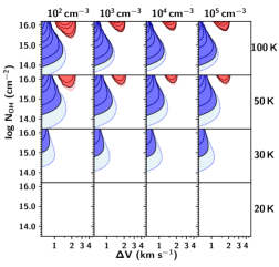
‘High’ Radiation: $T_{\rm dust}({\rm ext})=70$ K $A_{\mathrm{v}}({\rm ext})$ $=0.1$ mag

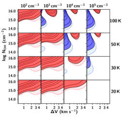
Figure 8: Same as the left panels of Fig. 6 without the effects of the radiation from internal dust.

In both radiation regimes there is a region of weak 1612 MHz inversion below $N_{\rm OH}/\Delta V\approx 2\times 10^{14}$ cm^-2 km^-1 s. This weak inversion is only seen when the effect of radiation from internal dust is included in our modelling, and cannot be replicated by simply increasing the column of external dust. (For comparison, Fig. 8 reproduces the left panels of Fig. 6 without the inclusion of internal dust.) The effect of the radiation from internal dust on the level populations of the first excited ${}^{2}\Pi_{3/2}\,J=5/2$ and the second excited ${}^{2}\Pi_{1/2}\,J=1/2$ rotational states (at $\lambda\approx 120\,{\rm\mu m}$ and 80 $\mu$m, respectively) is illustrated in Fig. 7. This figure shows the proportional change in population of the hyperfine levels within these two excited rotational states in the ‘low’ radiation regime, for a gas kinetic temperature of 30 K, number density of $10^{3}\,{\rm cm}^{-3}$ and velocity dispersion of 1.4 km s^-1. The population in all levels is increased when radiation from internal dust is included, and this increase is greatest for the second excited ${}^{2}\Pi_{1/2}\,J=1/2$ rotational state (shown in red in Fig. 7), which tends to invert the 1612 MHz line.

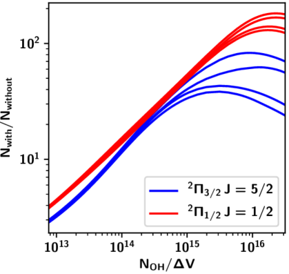
Figure 7: The ratio of level populations $N$ with the effects of internal dust and without as a function of $N_{\rm OH}/\Delta V$ for the hyperfine levels in the first excited ${}^{2}\Pi_{3/2}\,J=5/2$ rotational state (blue) and the second excited ${}^{2}\Pi_{1/2}\,J=1/2$ rotational state (red). The values shown represent a model cloud in the ‘low’ radiation regime (see Fig. 6) with gas kinetic temperature 30 K, number density $10^{3}\,{\rm cm}^{-3}$ and velocity dispersion 1.4 km s^-1.

The dominant pattern of 1720 MHz inversion seen in the low radiation regime (particularly in the lower gas temperature and number density panels) is qualitatively consistent with the fact that the 1720 MHz line is widely observed in emission in the ambient ISM of the Galactic Plane, in contrast to the 1612 MHz line which is more commonly seen in absorption (Turner, 1982; Dawson et al., 2014). Increasing the radiation field increases the range of column densities and velocity dispersions at which the 1612 MHz line will invert, and inhibits the 1720 MHz inversion at low gas temperatures and number densities, while still readily allowing 1720 MHz inversion at higher gas temperatures and number densities.

In the case of the 23 examples of the satellite-line flip where the 1720 MHz inversion is seen at more negative velocities, has a bright background source of continuum, and is associated on sky and in velocity with an Hii region, we may consider a model in which an Hii region provides the high radiation field required to invert the 1612 MHz line at typical molecular cloud gas temperatures and number densities. The expanding Hii region drives a shock into this molecular gas, as illustrated by the cartoon in Fig. 4. The moderate shock velocity ($<10$ km s^-1 Hosokawa & Inutsuka, 2005, 2006) will only partially dissociate the molecular gas (Draine et al., 1983; Flower et al., 2003). The increased gas temperature and number density of the shock pushes the post-shock gas into the collisionally dominated regime, disabling the 1612 MHz inversion and inverting the 1720 MHz line. This picture provides a very natural explanation for the observed features of the satellite line flip.

4 Discussion

The high-radiation case outlined above provides a qualitatively convincing explanation of the satellite line flip as a phenomenon driven by the expansion of an Hii region into a molecular cloud. The on-sky association of the majority of observed flips with known Hii regions, together with the systematic bias in velocity orientation (with 1720 MHz-inverted gas always approaching faster), paint very consistent parts of this picture. However, it is important to note that a satellite line flip can in principle be produced without the need for expansion, shocks, or a high IR radiation field. The basic requirements are only the presence of molecular gas on either side of a velocity discontinuity, with the gas on either side possessing sufficiently different physical parameters to invert the relevant lines. Our non-LTE modelling indeed shows that a flip could in principle be driven by changes in number density, column density, velocity dispersion or gas temperature, even in ambient low-radiation regions.

That said, of the two radiation fields considered in our modelling (illustrated in Fig. 6), a flip is more readily and comfortably produced in the ‘high’ radiation regime. In this scenario, increased FIR radiation allows the 1612 MHz inversion to be radiatively pumped in the pre-shock gas of the molecular cloud – in contrast to the 1720 MHz emission more generally seen in the ambient molecular ISM (Turner, 1982; Dawson et al., 2014). Our modelling has then shown that the increased temperature and number density of the post-shock gas can disable the 1612 MHz pumping mechanism and allow the 1720 MHz line to invert. These are both essential elements of our Hii region picture, which requires 1612 MHz emission from the ambient pre-shock gas, and 1720 MHz emission from a blue-shifted, shocked component.

Importantly, however, this high radiation regime also allows the 1612 MHz line to invert at lower column densities, permitting a lower line-of-sight extent for the 1612 MHz-inverted component of the flip. Assuming an ambient molecular cloud density of $n_{\rm H_{2}}\approx 10^{3}\,{\rm cm}^{-3}$ and an OH abundance relative to H₂ of $X_{\rm OH}=10^{-7}$, the column density of $N_{\rm OH}=10^{15.5}\,{\rm cm}^{-2}$ shown in the high radiation synthetic spectrum at the bottom right in Fig. 6 would require a line-of-sight extent of $\approx 10\,$pc. In contrast, the column density of $N_{\rm OH}=10^{16}\,{\rm cm}^{-2}$ shown in the low radiation synthetic spectrum would require a line-of-sight extent of $\approx 30$ pc. Both distances are problematic when we consider the velocity gradient of the ambient molecular cloud that is suggested by these values. The synthetic spectrum in the low radiation regime would require a velocity gradient of $\approx 0.04\,{\rm km\,s}^{-1}\,{\rm pc}^{-1}$, while that of the high radiation regime would require a velocity gradient of $\approx 0.12\,{\rm km\,s}^{-1}\,{\rm pc}^{-1}$: both significantly lower than the expected value of $1\,{\rm km\,s}^{-1}\,{\rm pc}^{-1}$ (Scoville & Solomon, 1974). We could of course make sensible increases to the ambient molecular cloud number density or the OH to H₂ abundance to produce a more acceptable velocity gradient, but such fine-tuning of a simplified 1D model may not be reasonable. It is difficult to evaluate this conclusion further without the support of more detailed or complex models.

Flip location		Velocity	Background		Refc
$l^{\circ}$	$b^{\circ}$	orientationa	continuumb
48.92	-0.28	1720 (-)	Extragalactic	41 K	1
172.80	-13.24	1612 (-)	CMB/synchrotron	4 K	2
173.40	-13.26	1612 (-)	CMB/synchrotron	4 K	3
175.83	-9.36	1612 (-)	CMB/synchrotron	4 K	1
336.95	-0.20	1720 (-)	Diffuse/unresolved	37 K	4

Table 3: Approximate 18 cm background brightness temperatures of the 5 instances of the satellite line flip not associated with Hii regions. ^aVelocity orientation of the flip is indicated by the line that is inverted at more negative velocities. ^bDescription of the background source of continuum and its brightness temperature at $\approx 18$ cm. ^cReferences: 1. Petzler et al. (2020 in prep), 2. Xu et al. (2016), 3. Ebisawa et al. (2019), 4. Dawson et al. (2014).

In our sample there are five instances of the flip without associated RRL detections. Table 3 lists their background brightness temperatures and restates their velocity orientations. First, we consider the flips with the more common velocity orientation (1720 MHz line inverted at more negative velocities), which are seen towards G048.92-0.28 (Petzler et al. 2020 in prep) and G336.95-0.20 ($-40\,$km s^-1, Dawson et al., 2014). Both of these sources lie in the Galactic Plane, have high background continuum temperatures and are positionally coincident with regions of active star formation. While they do not have literature RRL detections within 10 km s^-1 of either component of the flip, it seems likely that these examples may represent pre- and post-shock gas surrounding as-yet unidentified Hii regions.

Next, we consider the flips with the opposite velocity orientation (1612 MHz line inverted at more negative velocities), which are seen towards G172.80-13.24 (Xu et al., 2016), G173.40-13.26 (Ebisawa et al., 2019) and G175.83-9.36 (Petzler et al. 2020 in prep). All three of these examples are within the Taurus molecular cloud complex and have low background continuum brightness temperature ($T_{\rm c}\sim 4$ K). The flip towards G175.83-9.36 is seen in optical depth with the 1612 MHz emission at $\tau=-0.003$ and the 1720 MHz at $\tau=-0.03$ (Petzler et al. 2020 in prep). Our modelling indicates that such weak inversion of the 1612 MHz line is possible in the low radiation regime at quite low column density. The 1720 MHz inversion could also be readily produced in this radiation regime across a wide range of column densities. Our modelling does not suggest that this example of the flip implies the presence of an enhanced radiation field or a shock.

The other two examples in Taurus (G172.80-13.24 and G173.40-13.26) are both reported in brightness temperature only, and it is therefore possible that they are not in fact stimulated emission ($T_{\rm ex}<0$), but rather conventional thermal emission ($T_{\rm ex}>T_{\rm c}$). The pumping mechanisms outlined in Section 2 could still be responsible for the deviations from LTE in this gas, but such thermal emission would not correspond exactly to the regions of stimulated emission illustrated in Fig. 6. Ebisawa et al. (2019) have recently presented non-LTE excitation modelling similar to ours of the flip towards G173.40-13.26. Their modelling focused on the blue-shifted component of this flip. They assumed a ‘typical’ velocity dispersion of 1 km s^-1, and a dust temperature of 15 K based on IR observations (Flagey et al., 2009). They found that the sub-thermal excitation of the 1720 MHz line inferred from their observations was best fit by a model with extremely high external dust column density ($A_{\mathrm{v}}({\rm ext})$ $\approx 150$ mag), high OH column density ($N_{\rm OH}>10^{15.5}\,{\rm cm}^{-2}$) and low gas temperature ($T_{\rm gas}<30\,$K). However, they did not propose a physical mechanism by which such a high dust column could exist in Taurus.

A key difference between our modelling and that of Ebisawa et al. (2019) appears to be our inclusion of the effects of internal dust: when we remove this from our modelling, the weak 1612 MHz inversion seen at low column densities in the low radiation regime in Fig. 6 is not present. This weak 1612 MHz inversion is simultaneous with sub-thermal excitation of the 1720 MHz line, implying that the inclusion of internal dust may allow the observations of Ebisawa et al. (2019) to be modelled without the need for such a high external dust column. Indeed, we find that our modelling is able to approximately reproduce the observed brightness temperatures of their blue-shifted component (with the same beam-filling factor used by Ebisawa et al. (2019) of 0.1) in a low radiation environment.

The above discussion highlights the need for caution when considering the exact quantitative results of 1D molecular excitation modelling. There are several known factors that our modelling does not consider, such as the effects of turbulence, unresolved structure in the foreground gas, and uncertainties or errors in collisional rates. Indeed, new collision rates of OH and H₂ (Kłos et al., 2020) are systematically higher than those used of Offer et al. (1994) in our modelling. There are also other significant observational assumptions that we do not address, such as structure in the background continuum source (Engelke & Allen, 2019). Therefore the fine-tuning of our model parameters in order to match observations is not likely to be strictly valid. Nevertheless, the qualitative physical picture presented here is convincing: the satellite line flip is most commonly and readily produced in pre- and post-shock gas in the high-radiation environment surrounding an expanding Hii region.

5 Conclusions

In this work we present 30 examples from the literature of the OH satellite-line flip: a peculiar profile wherein both of the OH ground rotational state satellite lines flip – one from emission to absorption and the other the reverse – across a closely blended double feature. We note that with the exception of the three flips observed towards the Taurus molecular cloud, all are observed towards bright background continuum and have the same orientation in velocity: the 1720 MHz inversion is seen at more negative velocities and the 1612 MHz inversion at more positive velocities. In addition, we note that all save 5 are associated with radio recombination lines of Hii regions.

We find that the 1612 MHz inversion can be radiatively pumped in an environment with typical molecular cloud gas temperature of $T_{\rm gas}\approx 20$ – $30\,$K and number density of $n_{\rm H_{2}}\approx 10^{2}$ – $10^{3}\,{\rm cm}^{-3}$, that is exposed to a high radiation field. The 1720 MHz inversion can then originate in gas exposed to this same radiation field but with enhanced gas temperature ($T_{\rm gas}\approx 50$ – $100\,$K) and number density ($n_{\rm H_{2}}\approx 10^{4}$ – $10^{5}\,{\rm cm}^{-3}$). We demonstrate that these physical conditions can be realised by a shock expanding from a central Hii region: the Hii region provides the enhanced radiation field required to invert the 1612 MHz line in the pre-shock gas while the shock heats and compresses the gas sufficiently to invert the 1720 MHz line. The brightness of the central Hii region causes the foreground gas to dominate the observed brightness temperature spectra, so the 1720 MHz inversion in the post-shock gas is blue-shifted relative to the 1612 MHz inversion in the pre-shock gas. We support this model through our own non-LTE molecular excitation modelling, and with reference to observations (Okumura et al., 1996; Anderson et al., 2012; Deharveng et al., 2012) and modelling (Churchwell et al., 1990; Hosokawa & Inutsuka, 2005, 2006) of Hii regions and dust temperatures. The precise quantitative results of our simplified 1D modelling should be regarded with caution as our models do not account for the clumpy and filamentary structure, nor the effects of turbulent motions known to exist in molecular clouds. The inclusion of such mechanisms may allow us to more precisely match the observed OH spectra.

The results presented in this work have highlighted a potential new tool for pinpointing the locations and properties of molecular gas associated with Hii regions. In principle, observations of the OH satellite-line flip should allow us to characterise the physical conditions in the molecular gas interacting with numerous Hii regions throughout the Galactic Disk, providing information on kinematics, density and temperature. For example, the velocity spacing of the flip and modelling of the blue-shifted 1720 MHz inversion could then characterise the kinematics and physical conditions of the expanding shock. As a radio spectral line probe, the OH lines (like RRLs) allow us to see through the full depth of the Milky Way disk, and localise interaction sites at least in the spatio-velocity domain, if not in true 3D space as well. Cross-matching with multi-wavelength tracers of Hii regions in the Milky Way Disk would therefore allow us to paint a more complete picture of the interactions between Hii regions and molecular gas in the Milky Way. With a number of large-scale OH Galactic Plane surveys either published or underway (e.g. THOR; Beuther et al. 2016, SPLASH; Dawson et al. 2014, and GASKAP; Dickey et al. 2013), there is scope to identify far more examples of the satellite flip, and moreover to model the overall trends in all four transitions throughout large regions of the Milky Way.

Data Availability

The data underlying this article were obtained from Goss (1967), Manchester et al. (1970), Caswell & Robinson (1974), Turner (1979), van Langevelde et al. (1995), Frayer et al. (1998), Brooks & Whiteoak (2001), Dawson et al. (2014), Xu et al. (2016), Rugel et al. (2018), Ebisawa et al. (2019) and Ogbodo et al. (2020), as outlined in Table 1. Additional data from Petzler et al. (2020 in prep.) and from private communication will be shared on reasonable request to the corresponding author.

Appendix A Satellite-line inversion without internal dust

References

- Allen et al. (2012) Allen R. J., Ivette Rodríguez M., Black J. H., Booth R. S., 2012, AJ, 143, 97
- Allen et al. (2015) Allen R. J., Hogg D. E., Engelke P. D., 2015, AJ, 149, 123
- Anderson et al. (2012) Anderson L. D., et al., 2012, A&A, 542, A10
- Anderson et al. (2014) Anderson L. D., Bania T. M., Balser D. S., Cunningham V., Wenger T. V., Johnstone B. M., Armentrout W. P., 2014, ApJS, 212, 1
- Anderson et al. (2015) Anderson L. D., Armentrout W. P., Johnstone B. M., Bania T. M., Balser D. S., Wenger T. V., Cunningham V., 2015, ApJS, 221, 26
- Anderson et al. (2018) Anderson L. D., Armentrout W. P., Luisi M., Bania T. M., Balser D. S., Wenger T. V., 2018, ApJS, 234, 33
- Barrett (1964) Barrett A., 1964, IEEE Transactions on Antennas and Propagation, 12, 822
- Barriault et al. (2010) Barriault L., Joncas G., Lockman F. J., Martin P. G., 2010, MNRAS, 407, 2645
- Baud & Wouterloot (1980) Baud B., Wouterloot J. G. A., 1980, A&A, 90, 297
- Beuther et al. (2016) Beuther H., et al., 2016, A&A, 595, A32
- Brooks & Whiteoak (2001) Brooks K. J., Whiteoak J. B., 2001, MNRAS, 320, 465
- Brown et al. (1982) Brown J. M., Schubert J. E., Evenson K. M., Radford H. E., 1982, ApJ, 258, 899
- Caswell (1999) Caswell J. L., 1999, MNRAS, 308, 683
- Caswell & Haynes (1975) Caswell J. L., Haynes R. F., 1975, MNRAS, 173, 649
- Caswell & Robinson (1974) Caswell J. L., Robinson B. J., 1974, Australian Journal of Physics, 27, 629
- Chu (1976) Chu S. I., 1976, ApJ, 206, 640
- Churchwell et al. (1990) Churchwell E., Wolfire M. G., Wood D. O. S., 1990, ApJ, 354, 247
- Dawson et al. (2014) Dawson J. R., et al., 2014, MNRAS, 439, 1596
- Deharveng et al. (2012) Deharveng L., et al., 2012, A&A, 546, A74
- Destombes et al. (1977) Destombes J. L., Marliere C., Baudry A., Brillet J., 1977, A&A, 60, 55
- Dickey et al. (2013) Dickey J. M., et al., 2013, Publ. Astron. Soc. Australia, 30, e003
- Draine & Lee (1984) Draine B. T., Lee H. M., 1984, ApJ, 285, 89
- Draine et al. (1983) Draine B. T., Roberge W. G., Dalgarno A., 1983, ApJ, 264, 485
- Dupac et al. (2003) Dupac X., et al., 2003, A&A, 404, L11
- Ebisawa et al. (2019) Ebisawa Y., Sakai N., Menten K. M., Yamamoto S., 2019, ApJ, 871, 89
- Elitzur (1976) Elitzur M., 1976, ApJ, 203, 124
- Elitzur (1978) Elitzur M., 1978, A&A, 62, 305
- Elitzur (1992) Elitzur M., 1992, Astronomical Masers. Astrophysics and Space Science Library, Springer Netherlands
- Elitzur et al. (1976) Elitzur M., Goldreich P., Scoville N., 1976, ApJ, 205, 384
- Engelke & Allen (2019) Engelke P. D., Allen R. J., 2019, ApJ, 874, 49
- Flagey et al. (2009) Flagey N., et al., 2009, ApJ, 701, 1450
- Flower et al. (2003) Flower D., Le Bourlot J., Pineau des Forêts G., Cabrit S., 2003, Astrophysics and Space Science, 287, 183
- Frail et al. (1994) Frail D. A., Goss W. M., Slysh V. I., 1994, ApJ, 424, L111
- Frail et al. (1996) Frail D. A., Goss W. M., Reynoso E. M., Giacani E. B., Green A. J., Otrupcek R., 1996, AJ, 111, 1651
- Frayer et al. (1998) Frayer D. T., Seaquist E. R., Frail D. A., 1998, AJ, 115, 559
- Goss (1967) Goss W. M., 1967, PhD thesis, University of California, Berkeley.
- Goss (1968) Goss W. M., 1968, ApJS, 15, 131
- Grenier et al. (2005) Grenier I. A., Casandjian J.-M., Terrier R., 2005, Science, 307, 1292
- Guibert et al. (1978) Guibert J., Rieu N. Q., Elitzur M., 1978, A&A, 66, 395
- Heiles (1968) Heiles C. E., 1968, ApJ, 151, 919
- Heiles (1969) Heiles C., 1969, ApJ, 157, 123
- Hodge & Kennicutt (1983) Hodge P. W., Kennicutt R. C. J., 1983, AJ, 88, 296
- Hosokawa & Inutsuka (2005) Hosokawa T., Inutsuka S.-i., 2005, ApJ, 623, 917