A new tool for predicting the solar cycle: Correlation between flux transport at the equator and the poles

1 Introduction

sec:intro

Detailed studies of solar photospheric magnetic fields are crucial for understanding the origin and evolution of solar magnetic activity which impacts the manner in which global solar magnetic fields evolve and change. The long term evolution of global solar magnetic fields is eventually important in the context of the heliospheric environment (Schwenn, 2006a; Sasikumar Raja et al., 2019), space weather activity changes in near-Earth space (Schwenn, 2006b) and in understanding the terrestrial magnetosphere and ionosphere (Pulkkinen, 2007; Janardhan et al., 2015b; Ingale, Janardhan, and Bisoi, 2019). Typically the origin of the magnetic activity of the Sun, well known as the solar cycle and varying with a period of $\sim$11 years, is attributed to a cyclic process, operated by an interior solar dynamo, which generates toroidal fields by shearing pre-existing poloidal fields and eventually regenerating poloidal fields to complete the cyclic process (Charbonneau, 2010). The toroidal fields get amplified by differential rotation (Parker, 1955a) and rise through the turbulent convection zone to form sunspot pairs or bipolar magnetic regions (BMRs) (Parker, 1955b). The BMRs emerge typically at low solar latitudes, around 35^o North and South at the start of the solar cycle constituting sunspot groups of positive and negative polarity fluxes. However, due to the systematic tilt of BMRs with respect to the equator (Hale et al., 1919), caused by the action of the Coriolis force on the buoyantly rising toroidal magnetic flux tubes, one of the spots in BMRs leads the other in both hemispheres, commonly known as leading polarity flux. While the other sunspot is known as following polarity flux. These opposite sunspot polarity fluxes generally cancel among themselves and decay according to the Babcock-Leighton mechanism (Babcock, 1961; Leighton, 1969).

The remnant leading and following polarity fluxes are transported, respectively, towards the equator and the poles due to diffusion and advection (Wang, Nash, and Sheeley, 1989). The leading polarity fluxes cancel those from the opposite solar hemisphere, at the equator, while the following polarity fluxes cancel the existing, opposite polarity polar cap fields and impart a new polarity. The polarity of the polar cap field thereby reverses, creating polar cap fields with opposite polarity. This well known process is referred to as polar field reversal, and with the exception of cycle 24 when the field reversal was extremely unusual and asymmetric (Gopalswamy, Yashiro, and Akiyama, 2016; Janardhan et al., 2018), takes place at each solar maximum (Babcock, 1961). One can therefore expect that there should be a correlation between the net amount of flux cancelled at the equator and the net amount of flux transported to the poles. We thus, in this study, investigate the relationship between the net flux variations across the equator and the poles during the past four solar cycles, viz. Cycles 21–24.

The polar field strength at the end of a cycle is crucial for determining the strength of toroidal fields in the subsequent cycle and, in turn, the amplitude of the next sunspot cycle (Jiang et al., 2018). In fact, the strength of polar field at the cycle minimum shows a good empirical correlation with the amplitude of the next sunspot cycle (Schatten and Pesnell, 1993; Schatten, 2005), so it has been used as a proxy to estimate the amplitude of the subsequent cycle (Schatten et al., 1978; Sofia, Fox, and Schatten, 1998; Svalgaard, Cliver, and Kamide, 2005; Choudhuri, Chatterjee, and Jiang, 2007; Janardhan et al., 2015a). Generally, surface flux transport simulations (Wang, Nash, and Sheeley, 1989; Sheeley, 2005; Mackay and Yeates, 2012; Iijima et al., 2017; Upton and Hathaway, 2018; Jiang et al., 2018; Bhowmik and Nandy, 2018) have been used to estimate the strength of the polar field at the minimum of a cycle. However, the possible correlation, if there is any, between the net flux strength across the equator and at the poles, can also be used to estimate the polar field strength at the cycle minimum. We thus discuss, in this study, the role of this correlation for estimating the amplitude of the upcoming Sunspot Cycle 25.

1.1 Magnetic Butterfly Diagram

sec:mag-field The observational evidence of a correlation between the flux transport at the equator and the poles can be seen from a magnetic butterfly diagram. Figure butter shows a magnetic butterfly diagram. The diagram is basically a latitudinal map in time depicting the distribution of photospheric magnetic fields for the period from February 1975 (1975.12) – December 2017 (2018.00) or CR1625 – CR2197 covering Solar Cycles 21 – 24. A magnetic butterfly diagram is generated using photospheric magnetic field values obtained from Carrington Rotation (CR) averaged synoptic magnetograms. A full description about the synoptic maps used is given in the following section and also can be found in Janardhan, Bisoi, and Gosain (2010); Janardhan et al. (2015a, 2018). The procedure for generating the butterfly diagram is described briefly below, and more details can be found in Bisoi et al. (2014) and Janardhan et al. (2018).

The butterfly diagram depicts the evolution of sunspot activity and the generation or renewal of polar fields. A butterfly pattern of bipolar sunspot groups is clear from Fig.butter as their latitudes of emergence shift equatorward with the progression of the solar cycle. These bipolar regions constituting leading and trailing or following fluxes of opposite polarity are shown in red and green in Fig.butter for Cycle 21, respectively. It is seen from Fig.butter that the leading and following polarity fluxes in each hemisphere move equatorward and poleward, respectively. The leading polarity fluxes are mostly confined to the equatorial belt between 0^∘-35^∘. Further, mixed populations of the leading polarity fluxes from the opposite hemispheres can be seen in the latitude range -10^∘ and 10^∘ that shows the cross-equatorial movement of the leading polarity fluxes and their eventual cancellation near the equator.

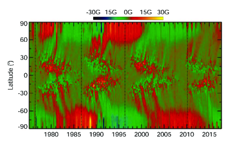
Figure 1.: A magnetic butterfly diagram shown, for the period 1975.14 – 2018.00, covering Solar Cycles 21 – 24. The magnetic flux has been limited to $\pm$30 Gauss so as to have better contrast and positive and negative polarities are shown in red and green respectively. The vertical dotted lines are drawn at solar minima of Cycles 20–23.butter

In the meanwhile, the following polarity fluxes in both hemispheres drift poleward and eventually reach the poles. This poleward motion of the trailing polarity fluxes can be seen from Fig.butter as tongues of flux, called polar surges, moving poleward in both hemispheres in the latitude band 45^∘-60^∘. The following polarity fluxes, or those moving poleward, eventually reach the poles, cancel the previous polar cap fluxes of opposite polarity (red, in Cycle 21) and impart a new polarity at the polar cap referred to as polar field reversal. It is, thus, clear from Fig.butter that the net flux transported to the equator or the amount of cross-equatorial flux could be correlated with the net flux transported to the poles. Again as the net flux transported to the poles is also correlated with the net amount of polar cap fields, the net amount of cross-equatorial flux could be related to polar cap fields. In this study, we thus investigate the possible correlations that could exist between the net flux transport at the equator and to the poles, and that between the net flux transport at the equator and polar cap fields.

2 Data and methodology

We used Carrington synoptic maps available from the magnetic database of the National Solar Observatory, Kitt Peak, USA (NSO/KP; ftp://nsokp.nso.edu/kpvt/synoptic/mag/) and the Synoptic Optical Long-term Investigation of the Sun facility (NSO/SOLIS; ftp://solis.nso.edu/synoptic/level3/vsm/merged/carr-rot/). A synoptic Carrington rotation map is generally made from several full-disk daily solar magnetograms observed over a CR period covering 27.2753 days. These maps, available online as standard FITS files contain 180 $\times$ 360 pixels in sine of latitude and longitude format.

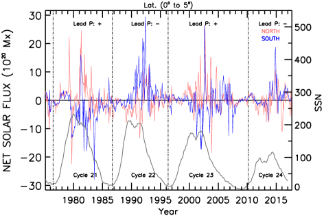
Figure 2.: The temporal variation of the net solar flux in the latitude range, 0^∘-5^∘, in the Northern (pink solid line) and Southern (blue solid line) hemispheres for Solar Cycles 21–24. Also, the temporal variations in SSN are shown by a grey solid line for the corresponding periods. The polarity of leading flux in the Northern hemisphere is indicated by a positive or negative sign at top of the figure. The vertical lines are drawn at each solar minimum.netf-0

For each synoptic map, photospheric magnetic fields were first estimated for each of the 180 arrays in sine of latitude by taking a longitudinal average of the entire 360 arrays of Carrington longitude. Thus, each CR map, previously in the form of an 180 $\times$ 360 array, is reduced to an array of 180 $\times$ 1. Similarly, such longitudinal strips of 180 $\times$ 1 were obtained for all synoptic maps in the period from 1975.14 to 2018.00 and a butterfly diagram was generated by placing each strip laterally in time. In short, the magnetic butterfly diagram represents latitudinal map of longitudinally averaged solar photospheric fields in time. Care was taken to see that data gaps, amounting to $\sim$2.5% of the total data set, were replaced with magnetic field values, estimated through a cubic spline interpolation (Janardhan, Bisoi, and Gosain, 2010). For achieving a better contrast in the butterfly diagram, the field strengths were restricted to $\pm 30$G, and the two polarities are shown respectively, in red (positive) and green (negative) in Fig.butter.

For the flux cancellation across the equator we estimate the net flux between the latitudes of $\pm$5^∘, while for the flux transport to the poles we estimate the net flux between the latitudes of $\pm$45^∘ and $\pm$60^∘. The magnetic flux density values for the desired latitude ranges were directly estimated from the magnetic butterfly diagram shown in Fig.butter. As mentioned earlier, the magnetic butterfly diagram comprises of an array of 180 $\times$573 in sine of latitude and time (in CR). For each time (in CR) we have 180 magnetic flux values in latitude. So to obtain the net magnetic flux in time for all CRs for a desired latitude range, for e.g. between latitude of 0^∘ and 5^∘, the (signed) magnetic fluxes are latitudinally averaged in the latitude bin of 0^∘ and 5^∘ separately for both the Northern and Southern hemispheres. We have particularly stressed in this paper the variation in the net magnetic flux at latitudes of 0^∘–5^∘, 45^∘–50^∘, 50^∘–55^∘, and 55^∘–60^∘, respectively. It is known (Hathaway, 2010) and evident from Fig.butter that the emergence of sunspots is largely confined to the the sunspot activity belt at latitudes between $\pm$5^∘ and $\pm$35^∘. Therefore, for the estimation of flux transport across the equator we have selected the latitudes of $\pm$5^∘, where the sunspots are barely seen. It is again known (Wang, Nash, and Sheeley, 1989; Mackay and Yeates, 2012) and evident from Fig.butter that the flux transport to the poles is mainly confined to the latitude range of $\pm$45^∘–$\pm$60^∘ where a series of discrete surges or tongues of flux are usually observed channelling the magnetic fluxes to the poles. Therefore, for the estimation of the flux transport to the poles we have selected the latitude range of $\pm$45^∘–$\pm$60^∘.

We estimated the polar cap fields measured above the latitude of 55^∘, which are actually the line-of-sight magnetic fields obtained from the Wilcox Solar Observatory (WSO) (http://wso.stanford.edu/Polar.html). A detail description about the WSO polar cap field measurements can be found in Janardhan et al. (2018). While for the monthly averaged total and hemispheric smoothed sunspot number (SSN), we used SSN V2.0 observations obtained from the Royal Observatory of Belgium, Brussels (http://www.sidc.be/silso/datafiles). The monthly total SSN observations are available since 1749, while the monthly hemispheric SSN ara available since only 1992. In this study, we thus used the monthly total SSN for Cycles 21–24 and monthly hemispheric SSN for Cycles 23-24. It is to be noted that a recalibrated SSN, known as SSN V2.0, was devised after Jul. 2015 (Clette and Lefèvre, 2016; Cliver, 2016) and is available at the Royal Observatory of Belgium.

3 Results and Discussions

sec:flux-var

3.1 Net flux variations at latitude of 0^∘- $\pm$5^∘

The net magnetic flux in the latitude band of 0^∘-5^∘ is shown in Figure netf-0. The pink and blue solid lines respectively represent temporal variation of magnetic measurements in the Northern and Southern hemispheres. The polarity of leading sunspot in the Northern hemisphere in each cycle is shown by a positive (+) or negative (-) sign at top in pink (parameters in the North are represented in pink and the South in blue). The net magnetic flux at the beginning of a cycle is generally less. This can be simply attributed to lower flux transport from the higher solar latitudes because at the start of the solar cycle sunspots have just started emerging at latitudes of $\pm$35^∘ in both hemispheres. The net flux then rises up gradually as the flux starts getting transported from the higher latitudes, and at the solar cycle maximum, the net flux is at the peak. Afterward, in the declining phase of the cycle, the net flux dips down because of the reduction in the number of sunspots, and the rise in flux cancellation at the equator. It is clearly seen from Figure netf-0 that the polarity of the net magnetic flux in both the hemispheres is same as that of the polarity of the leading sunspots in their respective hemispheres.

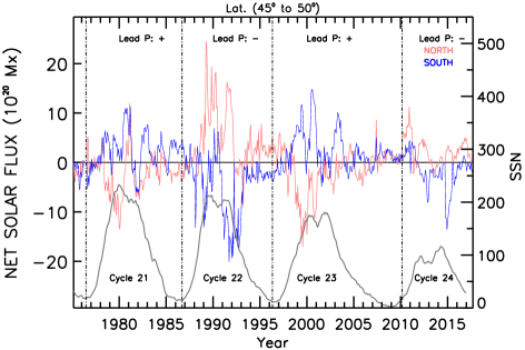
Figure 3.: The temporal variation of the net solar flux in latitude range, 45^∘-50^∘, for the Northern and Southern hemispheres marked in pink and blue, respectively, shown for Solar Cycles 21–24.netf-45

From the variation of the net hemispheric flux in the latitude band of 0^∘- $\pm$5^∘ the presence of the wrong orientation fluxes are also easily observable. As described earlier, we see that the bipolar sunspot regions generally follow the Hale’s polarity law (Hale et al., 1919) so that the leading and following spots have a polarity opposite to that of the corresponding polarity of the leading and following spots in the other hemisphere. However, it is sometimes found that bipolar regions have an orientation opposite to the normally expected orientation of bipolar regions. Such fluxes are referred to as wrong orientation fluxes (Wang, Nash, and Sheeley, 1989; Jiang, Cameron, and Schüssler, 2015). For example, in Cycle 21, we can clearly see sudden changes in the polarity of the net magnetic flux in the Northern hemisphere from positive to negative during the period around 1980. We also find a similar behaviour in the Southern hemisphere around the period 1982. Similarly, wrong orientation fluxes are also observed in Cycle 23 where the polarity of the net flux in the Southern hemisphere changes from positive to negative around 2004. Such changes in the polarity of net fluxes indicate the appearance of low latitude bipolar regions having the wrong orientation of fluxes.

A close inspection of the net flux variation in Cycle 24 shows a peculiarity in the Southern hemisphere. As expected, the polarity of the net flux in the beginning of the cycle was positive until 2012 while it was unexpectedly negative from 2012–2014, and only changed back to normal polarity when it approached solar cycle maximum. However, such behaviour of the net flux has not been noticed for other Solar Cycles 21–23 from the Southern hemisphere. Also, a comparison of the net magnetic flux variation in the Northern and Southern hemispheres in the last four Solar Cycles 21–24 shows a clear hemispheric asymmetry. However, it is important to note that this hemispheric asymmetry is much more significant in Cycle 22 as compared to other solar cycles wherein, the flux from the Southern hemisphere is seen significantly higher than that of the Northern hemisphere during the solar maximum of the cycle. A quantification of the hemispheric magnetic flux asymmetry is further discussed in Section sec:correlation.

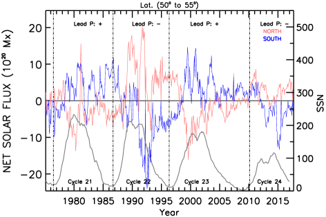
Figure 4.: The temporal variation of the net solar flux in latitude range, 50^∘-55^∘, for the Northern and Southern hemispheres marked in pink and blue, respectively, shown for Solar Cycles 21–24.netf-50

3.2 Net flux variations at latitude of $\pm$45^∘- $\pm$50^∘

sec:netf-45 The net flux in the latitude band of $\pm$45^∘–$\pm$50^∘ is shown in Figure netf-45 for both the Northern and Southern hemispheres. Unlike the latitude band of 0^∘-5^∘, the polarity of the net flux in each hemisphere is opposite to that of the polarity of leading sunspots. However, as mentioned for the latitude band of 0^∘–$\pm$5^∘, for this latitude band we also found changes in the polarity of the net flux. In particular it is seen that, such changes are comparatively more frequent in Cycles 21 and 23 compared to that of Cycles 22 and 24. In Cycle 21 a sudden large change in the polarity of the net flux is found in the North around 1980, while a similar change in the polarity of the net flux is observed at around 1982 in the South. These changes in the polarity of the net flux corresponds to the same period of time when changes in the polarity of the net flux have been observed in the latitude band of 0^∘- $\pm$5^∘. Thus, this further confirms the low latitude emergence of the bipolar magnetic regions with the wrong orientation. Similarly, we have also noticed, in Cycle 22, random changes in polarity of the flux in the South around the solar cycle maximum while the same has been noticed frequently in Cycle 23 both in the Northern and Southern hemispheres after the solar cycle maximum. In addition, the strength of the net hemispheric flux in Cycle 23 was comparatively less after around 2004,

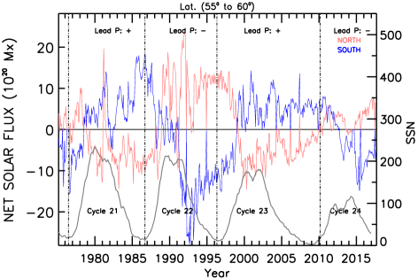
Figure 5.: The temporal variation of the net solar flux in the latitude range, 55^∘-60^∘, for both solar hemisphere, with the Northern and Southern hemispheres marked in pink and blue, respectively, shown for Solar Cycles 21–24.netf-55

and was subsequently reduced during the prolonged minimum of Cycle 23 indicating that the flux transport to the polar cap region was low. This may explain the weakness of polar field strength during the minimum of Cycle 23. Unlike the latitude band of 0^∘-$\pm$5^∘ the net flux in Cycle 24 shows a normal or expected behaviour though its strength is comparatively weaker.

Also, from Fig.netf-45, the hemispheric asymmetry in the net magnetic flux variation in each solar cycle is clearly evident and like the latitude band of 0^∘–$\pm$5^∘, the hemispheric asymmetry is more significant in Cycle 22. In addition, the same in Cycle 24 also shows significant difference during the maximum of Cycle 24 with the flux for the Southern hemisphere higher than that of the Northern hemisphere.

	Latitude	Solar Cycle	${\lvert\phi\rvert}_{N}$ ($\times$1022Mx)	${\lvert\phi\rvert}_{S}$ ($\times$1022Mx)	${\Gamma_{\Phi}}$
	0∘–5∘	21	1.29	3.61	0.47
		22	1.45	3.36	0.40
		23	1.93	1.21	0.23
		24	0.49	1.33	0.49
	45∘–50∘	21	3.00	3.07	0.01
		22	5.53	5.69	0.01
		23	3.03	3.97	0.13
		24	2.30	1.80	0.12
	50∘–55∘	21	3.68	4.29	0.07
		22	6.84	6.76	0.01
		23	3.70	4.54	0.11
		24	2.80	2.25	0.10
	55∘–60∘	21	5.05	5.52	0.04
		22	8.57	8.06	0.03
		23	4.34	5.02	0.07
		24	2.71	2.60	0.02

Table 1.: Lists the estimated net flux values for Solar Cycles 21–24 in the Northern (${\lvert\phi\rvert}_{N}$) and Southern (${\lvert\phi\rvert}_{S}$) hemispheres and the hemispheric magnetic flux asymmetry (${\Gamma_{\Phi}}$) in the latitude bands 0^∘- $\pm$5^∘, $\pm$45^∘- $\pm$50^∘, $\pm$50^∘- $\pm$55^∘, and $\pm$55^∘- $\pm$60^∘, respectively.tab-1

3.3 Net flux variations at latitude of $\pm$50^∘- $\pm$55^∘

sec:netf-50 The temporal variation in the net flux in latitude bin 50^∘-55^∘ is shown in Figure netf-50 both in the Northern and the Southern hemispheres. The variations seen show that they are almost similar in behaviour to the net flux variations seen in the latitude bin, 45^∘-50^∘. It is seen that the polarity of the net flux also behaves in the same way. The difference that distinguishes it from the previous latitude bin is that the strength of the net flux in every cycle is comparatively higher. Also, the abrupt changes in the polarity of the net flux that are seen during Solar Cycle 22 are for a longer duration than earlier and the strength of the net flux in the South is stronger. However, unlike the frequent changes of the polarity of the net flux (as seen in Cycles 21 and 23 in the previous latitude band of 45^∘ - 50^∘) we find such changes are less frequent in this latitude band. This indicates that both polarity fluxes are transported up to the latitude of $\pm$50^∘.

	Latitude		Hemisphere	Pearson’s Correlation	Spearman’s Correlation
	0∘–5∘	45∘–50∘	North	-0.26(P=99%)	0.50(P=66%)
			South	0.08 (P=99%)	-0.50(P=66%)
			North & South	0.10 (P=99%)	0.20(P=70%)
	0∘–5∘	50∘–55∘	North	-0.27 (P=99%)	0.5(P=66%)
			South	0.33 (P=99%)	-0.5(P=66%)
			North & South	0.21 (P=99%)	0.08(P=87%)
	0∘–5∘	55∘–60∘	North	-0.42 (P=99%)	-0.50(P=66%)
			South	0.55 (P=99%)	0.5(P=66%)
			North & South	0.22 (P=99%)	0.31(P=54%)
	0∘–5∘	55∘–90∘	North	-0.99 (P=99%)	-1.00(P=66%)
			South	0.87 (P=99%)	1.00(P=66%)
			North & South	0.51 (P=99%)	0.31(P=54%)

Table 2.: Lists the Pearson’s and Spearman’s rank correlations between the net flux values in the latitude bands of 0^∘-5^∘ and 45^∘-50^∘, 0^∘-5^∘ and 50^∘-55^∘, 0^∘-5^∘ and 55^∘-60^∘, 0^∘-5^∘and 55^∘-90^∘ for the Northern, Southern, and both hemispheres, estimated for Solar Cycles 21–23.tab-2

The hemispheric asymmetry in the net flux variation in each solar cycle for this latitude band shows a similar behaviour like that in the latitude band of 45^∘–50^∘.

3.4 Net flux variations at latitude of $\pm$55^∘- $\pm$60^∘

sec:netf-55 Figures netf-55 represents the net flux for both the Northern and Southern hemispheres in the latitude band of $\pm$55^∘-$\pm$60^∘. The net flux in this latitude bin, as depicted in Figure netf-55, is actually more like the polar cap flux, which shows a reversal in polarity of the flux in each cycle at around solar cycle maximum, unlike the net flux in the previous latitude bands. At the initial phase of solar cycle, the net hemispheric flux has the same polarity to that of the leading sunspot flux. As the solar cycle progresses the net hemispheric flux strength decreases and at around the solar maximum the polarity of the net hemispheric flux reverses, and is the same as that of the polarity of the following sunspot flux.

Actually, as pointed out previously, the surplus amount of trailing polarity fluxes transported from the low latitudes, on reaching in this regime, cancel the old polar cap flux to produce the new polar cap flux having the opposite polarity. A comparison of the strength of the net flux in this latitude band for Cycles 21 – 24 shows that the net flux was weaker during the prolonged minimum of Cycle 23 as compared to the earlier minima of Solar Cycles 20–22. The net flux in the rising phase of the Cycle 24 as well as in the declining phase of the Cycle 24 were also found weaker in strength as compared to the earlier cycles. Also, the hemispheric asymmetry in the net flux variation for each solar cycle, like in the previous latitude bands of 45^∘–50^∘ and 50^∘-55^∘, is clearly seen during the maxima of Cycles 22 and 24.

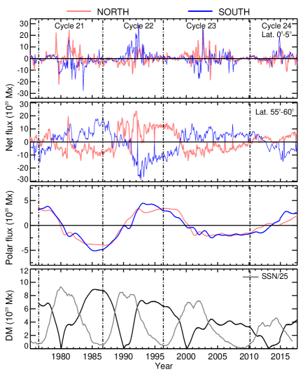
Figure 6.: (first and second panels) the temporal variation in the net solar flux in latitude range, 0^∘-5^∘ (first panel) and 55^∘-60^∘ (second panel) for the northern and southern hemispheres marked in pink and blue respectively for Solar Cycles 21-23. (third panel) the variation in the north polar cap flux (pink) and negative of south polar cap flux (blue) estimated from the WSO polar field measurements for the last four solar cycles. (fourth panel) the variation of axial dipole moment estimated from WSO polar fields (black) overplotted by the monthly averaged SSN (grey) divided by 25. The vertical lines demarcate the solar minima differentiating the solar cycles.netflux-0n55

3.5 Correlation of the net solar fluxes

sec:correlation From the investigation of variations in the net flux at different latitude bands, as described above, it is apparent that the flux cancelled across the equator and the flux transported to the poles may have a correlation. For finding the correlation between the net amount of flux in the latitude belt of 0^∘–$\pm$5^∘ with that of the corresponding net amount of flux in the latitude band $\pm$45^∘–$\pm$50^∘, $\pm$50^∘–$\pm$55^∘, and $\pm$55^∘–$\pm$60^∘, respectively, the net amount of flux in both the North and the South is estimated for each solar cycle from Cycles 21 – 24. The estimated fluxes in both the North and South for each solar cycle are listed in Table tab-1 for these latitude bands. We also estimated the magnetic flux asymmetry, ${\Gamma_{\Phi}}$:

$$\Gamma{{}_{\phi}}=\frac{{\lvert\phi\rvert}_{N}-{\lvert\phi\rvert}_{S}}{{\lvert\phi\rvert}_{N}+{\lvert\phi\rvert}_{S}}\ilabel{eqphi}$$ (1)

where ${\lvert\phi\rvert}_{N}$ and ${\lvert\phi\rvert}_{S}$ are absolute values of the net flux for the Northern and Southern hemispheres. The estimated values of ${\Gamma_{\Phi}}$ in each solar cycle are also listed in Table tab-1 for these latitude bands.

An inspection of the net flux values as shown in Table tab-1 reveals that the net amount of flux in the latitude band 0^∘–$\pm$5^∘ shows a progressive increase in its strength from Cycle 21 to 23 in the North while for the South it shows a reduction in its strength. However such behaviour has not been observed for all the other latitude bands, although it is noticed that the net flux shows a progressive decrease in its strength from Cycle 22 to 24 for both the North and South with the flux is higher in Cycle 22 in comparison to Cycles 21, 23 and 24. This suggests a continuous weaker polar flux since Cycle 22. It is to be reminded here that in our earlier studies (Janardhan, Bisoi, and Gosain, 2010; Janardhan et al., 2015a; Ingale, Janardhan, and Bisoi, 2019) we also showed a similar steady decrease in unsigned polar field strength since Cycle 22. While a comparison of the net flux values for the North and South in the latitude band 0^∘–$\pm$5^∘ shows a weaker net magnetic flux for the North in each solar cycle except for Cycle 23 wherein the net magnetic flux in the North is stronger than the South. Also, a lower value (0.23) of ${\Gamma_{\Phi}}$ has been found for Cycle 23 as compared to other Solar Cycles (0.40-0.49). On the other hand, the comparison of the net flux values for the North and South in the latitude band 45^∘–50^∘ shows a weaker net magnetic flux for the North in each solar cycle except for Cycle 24. In the latitude bands 50^∘–55^∘ and 55^∘–60^∘, the net flux values for the North and South are alternatively stronger or weaker from Cycles 21–24. While the inspection of ${\Gamma_{\Phi}}$ values for these latitude bands shows no specific trend. However, the value of ${\Gamma_{\Phi}}$ has been found to be comparatively higher for Cycle 23 as compared to other Solar Cycles.

We estimated the Pearson’s correlation coefficient and the Spearman’s rank correlation coefficient by comparing the net amount of flux in the Northern hemisphere in the latitude belt of 0^∘–$\pm$5^∘ with that of of the net flux in the latitude belt of $\pm$45^∘–$\pm$50^∘, $\pm$50^∘–$\pm$55^∘, and $\pm$55^∘–$\pm$60^∘, respectively. Similarly, we repeated the same for the Southern hemisphere too. All these estimated coefficient values are listed in Table tab-2 with their statistical significance. It is evident form Table tab-2 that a moderately good negative correlation (Pearson’s correlation coefficient, r = -0.42, P=99% confidence level) is observed between the net flux in the latitude band of 0^∘–5^∘ and 55^∘–60^∘ for the North while a moderately good positive correlation (Pearson’s correlation coefficient, r = 0.55, P=99%) is observed for the South. It thus indicates that the flux cancellation at the equator and the flux transport to the poles have a good correlation. When we consider the net flux values of the North and the South together to find any correlation between the latitude band of 0^∘–5^∘ and 55^∘–60^∘, we found low values of Pearson’s correlation coefficient (r=0.22, P=99%) and Spearman’s rank correlation coefficient ($\rho$=0.31, P=54%). Thus, it is clear that the correlation for the net flux only exists when the North and South are taken separately, but not for the net flux for the North and South considered together.

Taking advantage of the new correlation between the net flux cancelled at the equator and the net flux transported to the poles, we tried to see if any correlation exists between the net flux cancelled at the equator and the polar fields at solar minimum. This has been discussed in the following section.

3.6 Correlation of the net flux at the equator and the polar cap fields

sec:flux-cantr For an easier comparison of the net flux in the latitude band of 0^∘–5^∘ and 55^∘–60^∘ during the past four Solar Cycles 21–24, we plot the respective net flux, obtained from NSOKP magnetic field measurements, in the first and second panels of Figure netflux-0n55 for both the Northern (pink) and Southern (blue) hemispheres, respectively. The variation in the polar cap flux, obtained from WSO measurements, is shown in the third panel of

	Solar Cycle	Year	CR	PMF${{}_{min}^{n}}$ (N)	PMF${{}_{min}^{n}}$ (S)
	21	1986	1771-1783	-8.5	10.7
	22	1996	1905-1917	7.2	-6.9
	23	2008-2009	2072-2084	-3.6	4.0

Table 3.: Lists the estimated values of polar cap fields (PMF${{}_{min}^{n}}$) in the Northern and Southern hemispheres during the solar minima of Cycles 21–23. The values of polar fields are in unit of Gauss.tab-3

Fig.netflux-0n55. The polar cap fields for the Southern hemisphere (blue) have been inverted in order to compare them with the polar cap fields for the Northern hemisphere (pink). While the axial dipole moment, estimated from the absolute difference between the Northern and Southern WSO polar cap fields, is shown in the fourth panel. Over-plotted in the fourth panel is also the monthly averaged SSN in grey, which is divided by 25 to fit into the Y-axis. The dotted vertical lines in each panel of Fig.netflux-0n55 demarcate the solar minima of Cycles 20–23. As mentioned earlier, it is clear from the first and second panels of Fig.netflux-0n55 that the net flux at the equator and the poles in Cycle 22 is comparatively more than that in cycles 21 and 23. While the net flux in Cycle 24 both at the equator and the poles is lower than that of Cycle 23. The same is found for the polar cap field strength during solar minimum of each cycle (third panel of Fig.netflux-0n55) with the field strength in Cycle 24 showing weaker values than that in Cycle 23. Thus, there may be a correlation between the net flux at the equator during each cycle (EMFⁿ) and the polar cap fields at cycle minimum (PMF${{}_{min}^{n}}$).

In order to find the correlation, we estimated WSO polar cap field strength during each solar cycle minimum, from Cycles 21–23, by averaging the values of polar cap fields in each hemisphere for an interval of one year around each solar cycle minimum. The one year intervals (Wang, Robbrecht, and Sheeley, 2009) around the minima of Solar Cycles 21, 22, and 23 were chosen corresponding to CR periods of CR1771–1783, CR1905–1917, and CR2072–2084, respectively. The estimated values of hemispheric polar cap fields for Cycles 21–23 are listed in Table tab-3. We have then compared these values with the already estimated values of the net flux in the latitude band 0^∘–5^∘, those representing the flux cancelled at the equator, and found a good correlation with a Pearson’s correlation coefficient of r = 0.51 and P = 99% confidence level. Shown in the left panel of Figure corr is the correlation of EMFⁿ versus PMF${{}_{min}^{n}}$. The filled black dots in Fig.corr (left) represent data points for both the Northern and Southern hemispheres for Cycles 21–23. The solid black line in Fig.corr is a best fit to all the data points obtained using a least square residual method. The linear correlation of EMFⁿ and PMF${{}_{min}^{n}}$ can be represented by the following equation,

$$PMF{{}_{min}^{n}}=4.06\pm(0.2)+(1.28\pm 0.05)\times EMF{{}^{n}}\ilabel{eq1}$$ (2)

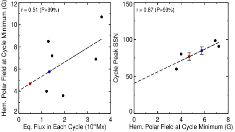
Figure 7.: (Left) correlation between net equatorial flux of each cycle with polar field at solar minimum shown with r=0.51 (P=99%). The filled black dots are data points for the Northern and Southern hemispheres covering Solar Cycles 21–23. The dashed line corresponds to a best fit obtained using the least square residual method. The filled red and blue dots are, respectively, values for the Northern and Southern hemisphere for Cycle 24. (Right) correlation between polar field at solar minimum of a preceding cycle and cycle peak of the following cycle shown with r=0.87 (P=99%). The filled black dots are data points for the Northern and Southern hemispheres for Cycles 22/23–23/24, while the filled red and blue dots represent the data point for the Northern and Southern hemispheres, respectively, for Cycle 24/25. The dashed line is a best fit to all the data points.corr

Using the values of EMFⁿ of 0.49 $\times$ 10²² Mx and 1.33 $\times$ 10²² Mx for the Northern and Southern hemispheres, respectively, for Cycle 24 (see Table tab-1) in Equation eq1, we estimated the values of PMF${{}_{min}^{n}}$ of 4.68 G and 5.76 G for the Northern and Southern hemispheres, respectively, for Cycle 24. The value for the North is indicated by a solid red circle in Fig.corr (left), while the value for the South is indicated by a solid blue circle.

An interesting feature in the correlation, when it is estimated separately for the North and South, is an improvement in the Pearson’s correlation coefficient. So for the North we found a Pearson’s correlation coefficient of r = -0.99 and P = 99%, while for the South we found a Pearson’s correlation coefficient of r = 0.87 and P = 99%.

3.7 Amplitude of solar cycle 25

sec:ampl25 Using polar flux measurements for Solar Cycles 14–23, Muñoz-Jaramillo, Balmaceda, and DeLuca (2013) showed that the solar cycle predictions made separately for each hemisphere provide a better estimate of SSN_max of the next cycle. Taking into this account, we used the estimated values of hemispheric PMF${{}_{min}^{n}}$ at Cycle 24 minimum to predict the amplitude of Solar Cycle 25 for the Northern and Southern hemispheres. We thus derived a correlation equation between hemispheric PMF${{}_{min}^{n}}$ and SSN${{}_{max}^{n+1}}$ using hemispheric measurements of PMF_min and SSN_max obtained for Solar Cycles 22 and 23, as shown in the right panel of Fig.corr. The filled solid dots in Fig.corr (right) represent the data points for Cycles 22-23. Although there are only four points, we found a very good statistically significant correlation between PMF${{}_{min}^{n}}$ and SSN${{}_{max}^{n+1}}$ with a Pearson correlation coefficient of $r=0.87$ at a significance level of $99\%$. Also, it is to be noted that the polar field strength at the minimum of a preceding cycle has been successfully used as a precursor for predicting the amplitude of the next cycle (Schatten et al., 1978; Schatten and Pesnell, 1993; Schatten, 2005) wherein the authors used either two or three data points only. The solid black line in Fig.corr (right) is a best fit to all the data points between PMF${{}_{min}^{n}}$ and SSN${{}_{max}^{n+1}}$. The linear correlation between them can be represented by the following equation,

$$SSN{{}_{max}^{n+1}}=40.78\pm(17)+(7.67\pm 3.0)\times PMF{{}_{min}^{n}}\ilabel{eq2}$$ (3)

Using the value of PMF${{}_{min}^{n}}$ of 4.68 G for the Northern hemisphere for Cycle 24 (see Section sec:flux-cantr) in equation eq2, we predict a SSN_max of 77$\pm$5 for Solar Cycle 25. This value is indicated by a solid red circle with a 1 sigma error-bar in Fig.corr (right). Similarly, using the value of PMF${{}_{min}^{n}}$ of 5.76 G for the Southern hemisphere for Cycle 24 in equation eq2, we predict a SSN_max of 85$\pm$5 for Solar Cycle 25. This value is indicated by a solid blue circle with 1 sigma error-bar in Fig.corr (right).

4 Summary and Conclusions

sec:con In this paper, we have used photospheric magnetic field measurements from NSOKP covering a period from Solar Cycles 21 – 24 to study and compare solar magnetic flux cancelled at the equator and transported to the poles. For the flux cancelled at the equator, we have estimated the net flux in the latitude belt $0^{\circ}$–$5^{\circ}$, while for the flux transported to the poles we have estimated the net flux in the latitude belt $45^{\circ}$–$50^{\circ}$, $50^{\circ}$–$55^{\circ}$, and $55^{\circ}$–$60^{\circ}$. We have estimated the net flux for each latitude belt for both the Northern and Southern hemispheres for each solar cycle from Cycles 21–24. The net flux variations in each latitude belt show different behaviour in each solar cycle, although an hemispheric asymmetry in the net flux strength is seen for each solar cycle in all the latitude belts. This asymmetry is more pronounced during the maximum of Cycle 22 as compared to the maxima of other cycles. While the value of hemispheric magnetic flux asymmetry for the latitude belt $0^{\circ}$–$5^{\circ}$ shows a lower value for Cycle 23 as compared to other solar cycles, the value of the same for all other latitude belts shows a higher value for Cycle 23 as compared to other solar cycles. Compared to earlier cycles both the flux cancelled at the equator and transported to the poles, in Cycle 24, show weaker hemispheric flux strength.

It is usually seen that the overall polarity of the net flux in each hemisphere is same as that of the leading sunspot polarity for the low latitude belt, while for the high latitude belt it is same as that of the following sunspot polarity. However, sometimes around the maximum of solar cycle, we have observed the change of polarity in the net flux transport at the equator, called as the wrong orientation fluxes, due to the emerging of low latitude rogue active regions. The same is also observed in the net flux estimated for the high latitude belts. This change of polarity due to the wrong orientation fluxes is different from the change in polarity of solar polar fields that usually always occurs during the maximum of each solar cycle. Such wrong orientation fluxes have been mostly seen in Cycles 21 and 23. It is argued (Jiang, Cameron, and Schüssler, 2015) that the wrong orientation fluxes seen during Cycle 23 have contributed to the weakness of Solar Cycle 24. Recently, Janardhan et al. (2018) reported the unusual polar field reversal pattern in Cycle 24 that showed a prolonged near-zero polar magnetic field condition in the Northern hemisphere after the start of the polar reversal. The multiple wrong orientation fluxes seen in Cycle 24, from this study, corresponding to the above period can explain the prolonged near-zero magnetic field condition in the Northern hemisphere.

Further, we have found a good correlation between the net flux in the latitude belt of $0^{\circ}$–$5^{\circ}$ and $55^{\circ}$–$60^{\circ}$ for the Northern as well as for the Southern hemispheres, and a much better correlation when we considered the net flux for both the Northern and Southern hemispheres together. Next, we have also compared the flux cancelled at the equator during each cycle to the polar cap field strength at the cycle minimum. We have found a good correlation between them when considered separately for the Northern and Southern hemispheres and together. We have used this correlation to estimate the hemispheric polar field strength at the Solar Cycle 24 minimum. The values, in turn, are used to estimate SSN_max of 77$\pm$5 and 85$\pm$5 for the Northern and Southern hemispheres, respectively, for the upcoming Solar Cycle 25. This is actually in agreement with the prediction made by Gopalswamy et al. (2018) wherein, the authors predicted SSN_max of 59 and 89 for the Northern and Southern hemispheres for Solar Cycle 25, respectively. The predicted values, from this study, for the amplitude of Solar Cycle 25 thus indicates that we would witness another mini-solar maximum, like that in Cycle 24, in the upcoming Solar Cycle 25. Janardhan et al. (2018) reported (see the upper panel of Fig.7 in the paper), that the strength of unsigned solar polar magnetic fields in the Southern hemisphere is relatively stronger than the Northern hemisphere in Solar Cycle 24. Thus, the amplitude of Solar Cycle 25 for the Southern hemisphere could be stronger than that for the Northern hemisphere that is exactly what our study reports here. In addition, it is shown in Fig.netflux-0n55 (third panel) of this study that an hemispheric asymmetry exists for the signed solar polar fields in Cycle 24 with the Southern polar fields reversing earlier than the Northern polar fields. This could lead to a delay in the timing of the sunspot minimum of Cycle 24 for the Northern hemisphere. As a result, there could be an hemispheric asymmetry in the timing of the sunspot maximum for the Northern and Southern hemispheres in the upcoming Solar Cycle 25.

In the present space age, the study of such evolution of solar photospheric magnetic flux and solar cycle predictions are important to plan the mission years of space and planetary exploration programs. Continued investigations of solar magnetic flux should thus be carried out.

Acknowledgement

The authors would thank the free use data policy of the National Solar Observatory (NSO/KP and NSO/SOLIS) and the Wilcox Solar Observatory (WSO) for the synoptic magnetogram data and World Data Center SILSO at Royal Observatory, Belgium, Brussels for the sunspot data. The SOLIS data obtained by the NSO Integrated Synoptic Program (NISP), managed by the National Solar Observatory, which is operated by the Association of Universities for Research in Astronomy (AURA), Inc. under a cooperative agreement with the National Science Foundation. Data storage supported by the University of Colorado Boulder “PetaLibrary.” SKB acknowledges Dr. Dibyendu Nandi from Indian Institute of Scientific and Educational Research (IISER), Kolkata for the scientific discussion and the support when the maximum work of this study has been carried out. Also, SKB acknowledges the support by the NSFC (Grant No. 11750110422, 11433006, 11790301, and 11790305).

References

- Babcock (1961) Babcock, H.W.: 1961, The Topology of the Sun’s Magnetic Field and the 22-YEAR Cycle. ApJ 133, 572. DOI. ADS.
- Bhowmik and Nandy (2018) Bhowmik, P., Nandy, D.: 2018, Prediction of the strength and timing of sunspot cycle 25 reveal decadal-scale space environmental conditions. Nature Communications. DOI.
- Bisoi et al. (2014) Bisoi, S.K., Janardhan, P., Chakrabarty, D., Ananthakrishnan, S., Divekar, A.: 2014, Changes in Quasi-periodic Variations of Solar Photospheric Fields: Precursor to the Deep Solar Minimum in Cycle 23? Sol. Phys. 289, 41. DOI. ADS.
- Charbonneau (2010) Charbonneau, P.: 2010, Dynamo Models of the Solar Cycle. Living Reviews in Solar Physics 7, 3. DOI. ADS.
- Choudhuri, Chatterjee, and Jiang (2007) Choudhuri, A.R., Chatterjee, P., Jiang, J.: 2007, Predicting Solar Cycle 24 With a Solar Dynamo Model. Physical Review Letters 98(13), 131103. DOI. ADS.
- Clette and Lefèvre (2016) Clette, F., Lefèvre, L.: 2016, The New Sunspot Number: Assembling All Corrections. Sol. Phys. 291, 2629. DOI. ADS.
- Cliver (2016) Cliver, E.W.: 2016, Comparison of New and Old Sunspot Number Time Series. Sol. Phys. 291, 2891. DOI. ADS.
- Gopalswamy, Yashiro, and Akiyama (2016) Gopalswamy, N., Yashiro, S., Akiyama, S.: 2016, Unusual Polar Conditions in Solar Cycle 24 and Their Implications for Cycle 25. ApJ 823, L15. DOI. ADS.
- Gopalswamy et al. (2018) Gopalswamy, N., Mäkelä, P., Yashiro, S., Akiyama, S.: 2018, Long-term solar activity studies using microwave imaging observations and prediction for cycle 25. Journal of Atmospheric and Solar-Terrestrial Physics 176, 26. DOI. ADS.
- Hale et al. (1919) Hale, G.E., Ellerman, F., Nicholson, S.B., Joy, A.H.: 1919,. ApJ 49, 153.
- Hathaway (2010) Hathaway, D.H.: 2010, The Solar Cycle. Living Reviews in Solar Physics 7(1), 1. DOI. ADS.
- Iijima et al. (2017) Iijima, H., Hotta, H., Imada, S., Kusano, K., Shiota, D.: 2017, Improvement of solar-cycle prediction: Plateau of solar axial dipole moment. A&A 607, L2. DOI. ADS.
- Ingale, Janardhan, and Bisoi (2019) Ingale, M., Janardhan, P., Bisoi, S.K.: 2019, Beyond the mini-solar maximum of solar cycle 24: Declining solar magnetic fields and the response of the terrestrial magnetosphere. Journal of Geophysical Research (Space Physics) 124, 6363. DOI. ADS.
- Janardhan, Bisoi, and Gosain (2010) Janardhan, P., Bisoi, S.K., Gosain, S.: 2010, Solar Polar Fields During Cycles 21 - 23: Correlation with Meridional Flows. Sol. Phys. 267, 267. DOI. ADS.
- Janardhan et al. (2015a) Janardhan, P., Bisoi, S.K., Ananthakrishnan, S., Tokumaru, M., Fujiki, K., Jose, L., Sridharan, R.: 2015a, A 20 year decline in solar photospheric magnetic fields: Inner-heliospheric signatures and possible implications. J. Geophys. Res. 120, 5306. DOI. ADS.
- Janardhan et al. (2015b) Janardhan, P., Bisoi, S.K., Ananthakrishnan, S., Sridharan, R., Jose, L.: 2015b, Solar and Interplanetary Signatures of a Maunder-like Grand Solar Minimum around the Corner - Implications to Near-Earth Space. Sun and Geosphere 10, 147. ADS.
- Janardhan et al. (2018) Janardhan, P., Fujiki, K., Ingale, M., Bisoi, S.K., Rout, D.: 2018, Solar cycle 24: An unusual polar field reversal. A&A 618, A148. DOI. ADS.
- Jiang, Cameron, and Schüssler (2015) Jiang, J., Cameron, R.H., Schüssler, M.: 2015, The Cause of the Weak Solar Cycle 24. ApJ 808, L28. DOI. ADS.
- Jiang et al. (2018) Jiang, J., Wang, J.-X., Jiao, Q.-R., Cao, J.-B.: 2018, Predictability of the Solar Cycle Over One Cycle. ApJ 863, 159. DOI. ADS.
- Leighton (1969) Leighton, R.B.: 1969, A Magneto-Kinematic Model of the Solar Cycle. ApJ 156, 1. DOI. ADS.
- Mackay and Yeates (2012) Mackay, D.H., Yeates, A.R.: 2012, The Sun’s Global Photospheric and Coronal Magnetic Fields: Observations and Models. Living Reviews in Solar Physics 9, 6. DOI. ADS.
- Muñoz-Jaramillo, Balmaceda, and DeLuca (2013) Muñoz-Jaramillo, A., Balmaceda, L.A., DeLuca, E.E.: 2013, Using the Dipolar and Quadrupolar Moments to Improve Solar-Cycle Predictions Based on the Polar Magnetic Fields. Physical Review Letters 111(4), 041106. DOI. ADS.
- Parker (1955a) Parker, E.N.: 1955a, Hydromagnetic Dynamo Models. ApJ 122, 293. DOI. ADS.
- Parker (1955b) Parker, E.N.: 1955b, The Formation of Sunspots from the Solar Toroidal Field. ApJ 121, 491. DOI. ADS.
- Pulkkinen (2007) Pulkkinen, T.: 2007, Space Weather: Terrestrial Perspective. Living Reviews in Solar Physics 4(1), 1. DOI. ADS.
- Sasikumar Raja et al. (2019) Sasikumar Raja, K., Janardhan, P., Bisoi, S.K., Ingale, M., Subramanian, P., Fujiki, K., Maksimovic, M.: 2019, Global Solar Magnetic Field and Interplanetary Scintillations During the Past Four Solar Cycles. Sol. Phys. 294, 123. DOI. ADS.
- Schatten (2005) Schatten, K.: 2005, Fair space weather for solar cycle 24. Geophys. Res. Lett. 32, 21106. DOI. ADS.
- Schatten and Pesnell (1993) Schatten, K.H., Pesnell, W.D.: 1993, An early solar dynamo prediction: Cycle 23 is approximately cycle 22. Geophys. Res. Lett. 20, 2275. DOI. ADS.
- Schatten et al. (1978) Schatten, K.H., Scherrer, P.H., Svalgaard, L., Wilcox, J.M.: 1978, Using dynamo theory to predict the sunspot number during solar cycle 21. Geophys. Res. Lett. 5, 411. DOI. ADS.
- Schwenn (2006a) Schwenn, R.: 2006a, Solar Wind Sources and Their Variations Over the Solar Cycle. Space Sci. Rev. 124(1-4), 51. DOI. ADS.
- Schwenn (2006b) Schwenn, R.: 2006b, Space Weather: The Solar Perspective. Living Reviews in Solar Physics 3(1), 2. DOI. ADS.
- Sheeley (2005) Sheeley, N.R. Jr.: 2005, Surface Evolution of the Sun’s Magnetic Field: A Historical Review of the Flux-Transport Mechanism. Living Reviews in Solar Physics 2, 5. DOI. ADS.
- Sofia, Fox, and Schatten (1998) Sofia, S., Fox, P., Schatten, K.: 1998, Forecast update for activity cycle 23 from a dynamo-based method. Geophys. Res. Lett. 25, 4149. DOI. ADS.
- Svalgaard, Cliver, and Kamide (2005) Svalgaard, L., Cliver, E.W., Kamide, Y.: 2005, Sunspot cycle 24: Smallest cycle in 100 years? Geophys. Res. Lett. 32, 1104. DOI. ADS.
- Upton and Hathaway (2018) Upton, L.A., Hathaway, D.H.: 2018, An Updated Solar Cycle 25 Prediction With AFT: The Modern Minimum. Geophys. Res. Lett. 45, 8091. DOI. ADS.
- Wang, Nash, and Sheeley (1989) Wang, Y.-M., Nash, A.G., Sheeley, N.R. Jr.: 1989, Evolution of the sun’s polar fields during sunspot cycle 21 - Poleward surges and long-term behavior. ApJ 347, 529. DOI. ADS.
- Wang, Robbrecht, and Sheeley (2009) Wang, Y.-M., Robbrecht, E., Sheeley, N.R. Jr.: 2009, On the Weakening of the Polar Magnetic Fields during Solar Cycle 23. ApJ 707, 1372. DOI. ADS.