On the Three Methods for Bounding the Rate of Convergence for some Continuous-time Markov Chains

Abstract. Consideration is given to the three different analytical methods for the computation of upper bounds for the rate of convergence to the limiting regime of one specific class of (in)homogeneous continuous-time Markov chains. This class is particularly suited to describe evolutions of the total number of customers in (in)homogeneous $M/M/S$ queueing systems with possibly state-dependent arrival and service intensities, batch arrivals and services. One of the methods is based on the logarithmic norm of a linear operator function; the other two rely on Lyapunov functions and differential inequalities, respectively. Less restrictive conditions (compared to those known from the literature) under which the methods are applicable, are being formulated. Two numerical examples are given. It is also shown that for homogeneous birth-death Markov processes defined on a finite state space with all transition rates being positive, all methods yield the same sharp upper bound.

Keywords: inhomogeneous continuous-time Markov chains, weak ergodicity, rate of convergence, sharp bounds, logarithmic norm, Lyapunov functions, differential inequalities, forward Kolmogorov system

1 Introduction

In this paper we revisit the problem of finding the upper bounds for the rate of convergence of (in)homogeneous continuous-time Markov chains. Consideration is given to classic inhomogeneous birth-death processes and to special inhomogeneous chains with transitions intensities, which do not depend on the current state. Specifically, let $\{X(t),\ t\geq 0\}$ be an inhomogeneous continuous-time Markov chain with the state space ${\mathcal{X}=\{0,1,2,\dots,S\}}$, where $1\leq S\leq\infty$. Denote by $p_{ij}(s,t)=P\left\{X(t)=j\left|X(s)=i\right.\right\}$, $i,j\geq 0,\;0\leq s\leq t$, the transition probabilities of $X(t)$ and by $p_{i}(t)=P\left\{X(t)=i\right\}$ – the probability that $X(t)$ is in state $i$ at time $t$. Let ${\mathbf{p}}(t)=\left(p_{0}(t),p_{1}(t),\dots,p_{S}(t)\right)^{T}$ be probability distribution vector at instant $t$. Throughout the paper it is assumed that in a small time interval $h$ the possible transitions and their associated probabilities are

$$p_{ij}(t,t+h)=\left\{\!\begin{array}[]{cc}q_{ij}(t)h\!+\!\alpha_{ij}\left(t,h\right),&\mbox{if }j\neq i,\\ 1\!-\!\sum\limits_{k\in\mathcal{X},k\neq i}q_{ik}(t)h\!+\!\alpha_{i}\left(t,h\right),&\mbox{if }j=i,\end{array}\right.$$

where transition intensities $q_{ij}(t)\geq 0$ are arbitrary non-random functions of $t$, locally integrable on $[0,\infty)$, satisfying $\sup_{i\in\mathcal{X}}\left(\sum_{k\in\mathcal{X},k\neq i}q_{ik}(t)\right)\leq L<\infty$ for almost all $t\geq 0$, and $|\alpha_{i}(t,h)|=o(h)$ for $S<\infty$ and $\sup_{i\in\mathcal{X}}|\alpha_{i}(t,h)|=o(h)$ for $S=\infty$. The results of this paper are applicable to Markov chains $X(t)$ with the following transition intensities:

1. $q_{ij}(t)=0$ for any $t\geq 0$ if $|i-j|>1$ and both $q_{i,i+1}(t)$ and $q_{i,i-1}(t)$ may depend on $i$;

2. $q_{i,i-k}(t)=0$ for $k\geq 2$, $q_{i,i-1}(t)$ may depend on $i$ and $q_{i,i+k}(t)$, $k\geq 1$, depend only on $k$;

3. $q_{i,i-k}(t)=0$ for $k\geq 1$ depend only on $k$, $q_{i,i+1}(t)$ may depend on $i$ and $q_{i,i+k}(t)=0$, $k\geq 2$;

4. both $q_{i,i-k}(t)$ and $q_{i,i+k}(t)$, $k\geq 1$, depend only on $k$ and do not depend on $i$.

Being motivated by the application of the obtained results in the theory of queues, in what follows it is convenient to think of $X(t)$ as of the process describing the evolution of the total number of customers of a queueing system. Then type (i) transitions describe Markovian queues with possibly state-dependent arrival and service intensities (for example, the classic $M_{t}(n)/M_{t}(n)/1$ queue); type (ii) transitions allow consideration of Markovian queues with state-independent batch arrivals and state-dependent service intensity; type (iii) transitions lead to Markovian queues with possible state-dependent arrival intensity and state-independent batch service; type (iv) transitions describe Markovian queues with state-independent batch arrivals and batch service. For the details concerning possible applications of Markovian queues with time-dependent transitions we can refer to [24], which contains a broad overview and a classification of time-dependent queueing systems considered up to 2016 and also [3, 4, 5, 24, 32, 34, 27, 19, 28, 9, 1, 17, 2, 25] and references therein.

In this paper we propose three different analytical methods for the computation of the upper bounds for the rate of convergence to the limiting regime (provided that it exists) of any process $X(t)$ belonging to one of the classes (i)–(iv). The first one is based on logarithmic norm of a linear operator function. The second one uses simplest Lyapunov functions and the third one relies on the differential inequalities. Even though the methods are not new, it is the first time when it is shown how they can be applied for the analysis of Markov chains with the transition intensities specified by (i)–(iv). This constitutes the main contribution of the paper. Another contribution is the fact that in a case of periodic intensities the bounds on the rate of convergence depend on the intensities only through their mean values over one period.

It is worth noticing here that, except for the upper bounds for the rate of convergence, we may also be interested in the lower bounds, stability (perturbation) bounds or truncation bounds (with error estimation). But the exact estimates of the rate of convergence yield exact estimates of stability bounds (see, for example, [7, 10, 14, 15, 20, 29, 16] and references therein). Moreover, as our research shows (see [32, 33, 34, 39]), in some cases, all these quantities can be constructed automatically, given that some good upper bounds for the rate of convergence are provided. This makes us believe that the upper bounds are of primary interest.

Estimation of the convergence rate by virtue of the methods proposed in this paper heavily relies on the notion of the reduced intensity matrix, say $B(t)$, of a Markov chain $X(t)$. The matrix $B(t)$ can be obtained by considering the probabilistic dynamics of the process $X(t)$, given by the forward Kolmogorov system

$$\frac{d}{dt}{\mathbf{p}}(t)=A(t){\mathbf{p}}(t),$$ (1)

where $A(t)$ is the transposed intensity matrix i.e. $a_{ij}(t)=q_{ji}(t)$, $i,j\in\mathcal{X}$. Since due to the normalization condition $p_{0}(t)=1-\sum_{i=1}^{S}p_{i}(t)$, we can rewrite the system (1) as follows:

$$\frac{d}{dt}{{\mathbf{z}}}(t)=B(t){{\mathbf{z}}}(t)+{{\mathbf{f}}}(t),$$ (2)

where

$${{\mathbf{f}}}(t)=\left(a_{10}(t),a_{20}(t),\dots\right)^{T},\ {{\mathbf{z}}}(t)=\left(p_{1}(t),p_{2}(t),\dots\right)^{T},$$

$${\footnotesize\!B(t)\!=\!\left(\begin{array}[]{ccccc}a_{11}\!-\!a_{10}&a_{12}\!-\!a_{10}&\cdots&a_{1r}\!-\!a_{10}&\cdots\\ a_{21}\!-\!a_{20}&a_{22}\!-\!a_{20}&\cdots&a_{2r}\!-\!a_{20}&\cdots\\ \cdots&\cdots&\cdots&\cdots&\cdots\\ a_{r1}\!-\!a_{r0}&a_{r2}\!-\!a_{r0}&\cdots&a_{rr}\!-\!a_{r0}&\cdots\\ \vdots&\vdots&\vdots&\vdots&\ddots\end{array}\right)\!.}$$ (3)

Here and henceforth each entry of $B(t)$ may depend on $t$ but, for the sake of brevity, the argument is omitted. We note that the matrix $B(t)$ has no any probabilistic meaning. All bounds of the rate of convergence to the limiting regime for $X(t)$ correspond to the same bounds of the solutions of the system

$$\frac{d}{dt}{{\mathbf{y}}}(t)=B(t){{\mathbf{y}}}(t),$$ (4)

because ${{\mathbf{y}}}(t)={{\mathbf{z}}}^{*}(t)-{{\mathbf{z}}}^{**}(t)$ is the difference of two solutions of system (2), and ${{\mathbf{y}}}(t)=\left({y}_{1}(t),{y}_{2}(t),\dots,{y}_{S}(t)\right)^{T}$ is the vector with the coordinates of arbitrary signs. As it was firstly noticed in [30], it is more convenient to study the rate of convergence using the transformed version $B^{*}(t)$ of $B(t)$ given by $B^{*}(t)=TB(t)T^{-1}$, where $T$ is the $S\times S$ upper triangular matrix of the form

$$T=\left(\begin{array}[]{ccccccc}1&1&1&\cdots&1\\ 0&1&1&\cdots&1\\ 0&0&1&\cdots&1\\ \vdots&\vdots&\vdots&\ddots\\ 0&0&0&\cdots&1\end{array}\right).$$ (5)

Let ${{\mathbf{u}}}(t)=T{{\mathbf{y}}}(t)$. Then the system (4) can be rewritten in the form

$$\frac{d}{dt}{{\mathbf{u}}}(t)=B^{*}(t){{\mathbf{u}}}(t),$$ (6)

where ${{\mathbf{u}}}(t)=\left({u}_{1}(t),u_{2}(t),\dots,u_{S}(t)\right)^{T}$ is the vector with the coordinates of arbitrary signs. If one of the two matrices $B^{*}(t)$ or $B(t)$ is known, the other is also (uniquely) defined.

The method based on the logarithmic norm of a linear operator function and the corresponding bounds for the Cauchy operator of reduced forward Kolmogorov system has already been applied successfully in many settings (see, for example, [5, 32]). Moreover, in [39] we have obtained the bounds for the rate of convergence and perturbation bounds for a process $X(t)$ belonging to classes (i)–(iv) under the assumption that $B^{*}(t)$ is essentially non-negative i.e. $b^{*}_{ij}(t)\geq 0$, $i\neq j$, $i,j\in\mathcal{X}\backslash(0)$. The obtained bounds are sharp for non-negative difference of the initial probability distributions of $X(t)$. In this paper it is no longer assumed that $B^{*}(t)$ must be essentially non-negative. Thus the considered class of eligible processes $X(t)$ is wider than the one considered in [39].

It may happen that the difference of the initial probability distributions of $X(t)$ has coordinates of different signs and/or $B^{*}(t)$ contains negative elements. In such situations the upper bounds provided by the method based on the logarithmic norm may not be sharp. Having alternative estimates, provided by the other two methods considered in this paper, we can choose the best. The idea to apply Lyapunov functions for the analysis of Markov chains is not new (see, for example, [6, 11]). Yet, to our best knowledge, in the considered setting they have not been applied before (see the seminal paper [41]). The approach based on the differential inequalities (see [42]) seems to be the most general: it can be applied both in the case when $B(t)$ is essentially non-negative (and yield the same results as the method based on the logarithmic norm) and in other cases in which the other two methods are not applicable. Usually the three methods lead to different upper bounds and the quality (sharpness) of the bounds depends on the properties of $B^{*}(t)$. All three methods are applicable when the state space i.e. $S<\infty$. For countable $\mathcal{X}$ the method based on Lyapunov functions no longer applies. Note also that for a $X(t)$ with a finite state space belonging to classes (i)–(iv) apparently no general method for the construction of Lyapunov functions can be suggested. Thus here consideration is given only to such $X(t)$, for which it can be guessed how Lyapunov functions can be constructed.

The paper is structured as follows. In the next section the explicit forms of the reduced intensity matrix $B^{*}(t)$ for each class (i)–(iv) are given. In section 3 we review the upper bounds on the rate of convergence, obtained by the method based on the logarithmic norm. Alternative upper bounds provided by Lyapunov functions and differential inequalities for some $X(t)$ from classes (i)–(iv) are given in sections 4 and 5. Section 6 concludes the paper.

2 Explicit forms of the reduced intensity matrix

As it was mentioned above, estimation of the convergence rate of $X(t)$ to the limiting regime is based on the reduced intensity matrix $B(t)$, given by (3), or its transform $B^{*}(t)=TB(t)T^{-1}$. In this section the explicit form of $B^{*}(t)$ for each class (i)–(iv) is given.

2.1 $B^{*}(t)$ for $X(t)$ belonging to class $\rm(i)$

Consider a process $X(t)$ with $a_{ij}(t)=0$ for any $t\geq 0$ if $|i-j|>1$, $a_{i,i+1}(t)=\mu_{i+1}(t)$ and $a_{i+1,i}(t)=\lambda_{i}(t)$. Then $X(t)$ is the inhomogeneous birth-death process with state-dependent transition intensities $\lambda_{i}(t)$ (birth) and $\mu_{i+1}(t)$ (death). In the queueing theory context, $X(t)$ describes the evolution of the total number of customers in the $M_{n}(t)/M_{n}(t)/1/S$ queue. For such $X(t)$ in the case of countable state space (i.e. $S=\infty$) the matrix $B^{*}(t)$ has the form:

$$B^{*}(t)=$$

$${\tiny\left(\begin{array}[]{ccccccc}-\left(\lambda_{0}+\mu_{1}\right)&\mu_{1}&0&\cdots&0&\cdots&\cdots\\ \lambda_{1}&-\left(\lambda_{1}+\mu_{2}\right)&\mu_{2}&\cdots&0&\cdots&\cdots\\ \ddots&\ddots&\ddots&\ddots&\ddots&\cdots\\ 0&\cdots&\cdots&\lambda_{r-1}&-\left(\lambda_{r-1}+\mu_{r}\right)&\mu_{r}&\cdots\\ \cdots&\cdots&\cdots&\cdots&\cdots&\cdots&\cdots\\ \end{array}\right).}$$ (7)

In the case of finite state space (i.e. $S<\infty$) the matrix $B^{*}(t)=$

$${\scriptsize\left(\begin{array}[]{ccccc}-\left(\lambda_{0}+\mu_{1}\right)&\mu_{1}&0&\cdots&0\\ \lambda_{1}&-\left(\lambda_{1}+\mu_{2}\right)&\mu_{2}&\cdots&0\\ \ddots&\ddots&\ddots&\ddots&\ddots\\ 0&\cdots&\cdots&\lambda_{S-1}&-\left(\lambda_{S-1}+\mu_{S}\right)\end{array}\right).}$$ (8)

Note that the matrix $B^{*}(t)$ is essentially non-negative for any $t\geq 0$ i.e. all its off-diagonal elements are non-negative for any $t$.

2.2 $B^{*}(t)$ for $X(t)$ belonging to class $\rm(ii)$

Consider a process $X(t)$ with $a_{ij}(t)=0$ for $i<j-1$, $a_{i+k,i}(t)=a_{k}(t)$ for $k\geq 1$ and $a_{i,i+1}(t)=\mu_{i+1}(t)$. Such $X(t)$ describes the evolution of the total number of customers in a queue with batch arrivals and single services ($a_{k}(t)$ are the (state-independent) intensities of group arrivals and $\mu_{i+1}(t)$ are the (state-dependent) service intensities). Such processes in the simplest forms were firstly considered in [18] and, under the assumption of decreasing of $a_{k}(t)$, have been studied in [39]. In the case of countable state space (i.e. $S=\infty$) the matrix $B^{*}(t)$ has the form:

$${\scriptsize B^{*}(t)=\left(\begin{array}[]{cccccc}a_{11}&\mu_{1}&0&\cdots&0\\ a_{1}&a_{22}&\mu_{2}&\cdots&0\\ a_{2}&a_{1}&a_{33}&\mu_{3}&\cdots&\\ \ddots&\ddots&\ddots&\ddots&\ddots\\ \ddots&\ddots&\ddots&\ddots&\ddots\\ \end{array}\right)}.$$ (9)

In the case of finite state space (i.e. $S<\infty$) the matrix $B^{*}(t)=$

$${\scriptsize\left(\begin{array}[]{ccccc}a_{11}-a_{S}&\mu_{1}&0&\cdots&0\\ a_{1}-a_{S}&a_{22}-a_{S-1}&\mu_{2}&\cdots&0\\ \ddots&\ddots&\ddots&\ddots&\ddots\\ a_{S-1}-a_{S}&\cdots&\cdots&a_{1}-a_{2}&a_{SS}-a_{1}\end{array}\right)}.$$ (10)

Note that the matrix $B^{*}(t)$ is essentially non-negative for any $t\geq 0$ if the arrival intensities $a_{k}(t)$ are decreasing in $k$.

2.3 $B^{*}(t)$ for $X(t)$ belonging to class $\rm(iii)$

Consider a process $X(t)$ with $a_{ij}(t)=0$ for $i>j+1$, $a_{i,i+k}(t)=b_{k}(t)$, $k\geq 1$ and $a_{i+1,i}(t)=\lambda_{i}(t)$. Such $X(t)$ describes the evolution of the total number of customers in a queue with batch services and single arrivals ($\lambda_{i}(t)$ are the (state-independent) arrival intensities and $b_{k}(t)$ are the (state-independent) intensities of service of a group of $k$ customers). Such processes were considered to some extent in [18, 8]. In the case of countable state space (i.e. $S=\infty$) the matrix $B^{*}(t)=$

$${\tiny\left(\begin{array}[]{cccccc}-\left(\lambda_{0}+b_{1}\right)&b_{1}-b_{2}&b_{2}-b_{3}&\cdots&\cdots\\ \lambda_{1}&-\big{(}\lambda_{1}+\sum\limits_{i\leq 2}b_{i}\big{)}&b_{1}-b_{3}&\cdots&\cdots\\ \ddots&\ddots&\ddots&\ddots&\ddots\\ 0&\cdots&\cdots&\lambda_{r-1}&-\big{(}\lambda_{r-1}+\sum\limits_{i\leq r}b_{i}\big{)}\cdots\\ \ddots&\ddots&\ddots&\ddots&\ddots\\ \end{array}\right)}.$$ (11)

In the case of finite state space (i.e. $S<\infty$) the matrix $B^{*}(t)$ is

$$B^{*}(t)=$$

$${\tiny\left(\begin{array}[]{ccccc}-\left(\lambda_{0}+b_{1}\right)&b_{1}-b_{2}&b_{2}-b_{3}&\cdots&b_{S-1}-b_{S}\\ \lambda_{1}&-\big{(}\lambda_{1}+\sum\limits_{i\leq 2}b_{i}\big{)}&b_{1}-b_{3}&\cdots&b_{S-2}-b_{S}\\ \ddots&\ddots&\ddots&\ddots&\ddots\\ 0&\cdots&\cdots&\lambda_{S-1}&-\big{(}\lambda_{S-1}+\sum\limits_{i\leq S}b_{i}\big{)}\end{array}\right)}.$$ (12)

Note that the matrix $B^{*}(t)$ is essentially non-negative for any $t\geq 0$ if the service intensities $b_{k}(t)$ are decreasing in $k$.

2.4 $B^{*}(t)$ for $X(t)$ belonging to class $\rm(iv)$

Consider a process $X(t)$ with $a_{i+k,i}(t)=a_{k}(t)$ and $a_{i,i+k}(t)=b_{k}(t)$ for ${k\geq 1}$. Such $X(t)$ describes the evolution of the total number of customers in an inhomogeneous queue with (state-independent) batch arrivals and group services ($a_{k}(t)$ are the (state-independent) intensities of group arrivals and $b_{k}(t)$ are the (state-independent) intensities of group services). Such process under the assumption of decreasing in $k$ intensities $a_{k}(t)$ and $b_{k}(t)$ have been studied in [34]. In the case of countable state space (i.e. $S=\infty$) the matrix $B^{*}(t)$ has the form:

$$B^{*}={\small\left(\begin{array}[]{cccccc}a_{11}&b_{1}-b_{2}&b_{2}-b_{3}&\cdots&\cdots\\ a_{1}&a_{22}&b_{1}-b_{3}&\cdots&\cdots\\ \\ \ddots&\ddots&\ddots&\ddots&\ddots\\ a_{r-1}&\cdots&\cdots&a_{1}&a_{rr}&\cdots\\ \cdots&\cdots&\cdots&\cdots&\cdots&\cdots\\ \end{array}\right)}.$$ (13)

In the case of finite state space (i.e. $S<\infty$) the matrix $B^{*}(t)=$

$${\small\left(\begin{array}[]{ccccc}a_{11}-a_{S}&b_{1}-b_{2}&b_{2}-b_{3}&\cdots&b_{S-1}-b_{S}\\ a_{1}-a_{S}&a_{22}-a_{S-1}&b_{1}-b_{3}&\cdots&b_{S-2}-b_{S}\\ \ddots&\ddots&\ddots&\ddots&\ddots\\ a_{S-1}-a_{S}&\cdots&\cdots&a_{1}-a_{2}&a_{SS}-a_{1}\end{array}\right)}.$$ (14)

Note that the matrix $B^{*}(t)$ is essentially non-negative for any $t\geq 0$ if the intensities $a_{k}(t)$ and $b_{k}(t)$ are decreasing in $k$.

3 Upper bounds using logarithmic norm

Throughout this section by $\|\cdot\|$ we denote the $l_{1}$-norm, i.e. $\|{{\mathbf{p}}(t)}\|=\sum_{i\in\mathcal{X}}|p_{i}(t)|$ and $\|A(t)\|=\sup_{j\in\mathcal{X}}\sum_{i\in\mathcal{X}}|a_{ij}(t)|$. Let $\Omega$ be a set of all stochastic vectors, i.e. $l_{1}$ vectors with non-negative coordinates and unit norm. Recall that a Markov chain $X(t)$ is called weakly ergodic, if ${\|{\mathbf{p}}^{*}(t)-{\mathbf{p}}^{**}(t)\|\to 0}$ as $t\to\infty$ for any initial conditions ${\mathbf{p}}^{*}(0)$ and ${\mathbf{p}}^{**}(0)$, where ${\mathbf{p}}^{*}(t)$ and ${\mathbf{p}}^{**}(t)$ are the corresponding solutions of (1).

Recall that the logarithmic norm of the operator function ${B}(t)$ is defined as

$$\gamma({B}(t))=\lim_{h\to+0}h^{-1}\left(\|I+hB(t)\|-1\right).$$

Denote by $V(t,s)=V(t)V^{-1}(s)$ the Cauchy operator of the equation (4). Then $\|V(t,s)\|\leq e^{\,\int_{s}^{t}\gamma(B(u))\,du}$. For an operator function from $l_{1}$ to itself we have the formula

$$\gamma({B}(t))=\sup_{j\in\mathcal{X}}\left(b_{jj}(t)+\sum_{i\in\mathcal{X},i\neq j}|b_{ij}(t)|\right).$$ (15)

Note that if the matrix $B(t)$ is essentially non-negative then $\gamma({B}(t))=\sup_{j\in\mathcal{X}}\left(\sum_{i\in\mathcal{X}}b_{ij}(t)\right)$.

Assume that the state space $\mathcal{X}$ is countable i.e. $S=\infty$. Let ${\{d_{i},\ i\geq 1\}}$ be a sequence of positive numbers and let $D=diag(d_{1},d_{2},\dots)$ be the diagonal matrix, with the off-diagonal elements equal to zero. By putting ${\bf w}(t)=D{\bf u}(t)$ in (6), we obtain the following equation

$$\frac{d}{dt}{\bf w}(t)=B^{**}(t){\bf w}(t),$$ (16)

where $B^{**}(t)=DB(t)^{*}D^{-1}$. Put

$$\alpha_{i}\left(t\right)=-\sum_{j=1}^{\infty}b_{ji}^{**}(t),\ i\geq 1,$$ (17)

and let $\alpha(t)$ and $\beta(t)$ denote the least lower and the least upper bound of the sequence of functions $\{\alpha_{i}(t),\ i\geq 1\}$ i.e.

$$\alpha\left(t\right)=\inf_{i\geq 1}\alpha_{i}\left(t\right),\ \beta\left(t\right)=\sup_{i\geq 1}\alpha_{i}\left(t\right).$$ (18)

The next theorem and corollary have been proved in [39, Theorem 1] and are stated here for the sake of completeness.

Theorem 1.

Let there exist a sequence $\{d_{i},\ i\geq 1\}$ of positive numbers such that $d_{1}=1$, $d=\inf_{i\geq 1}d_{i}>0$ and $B^{*}(t)$ is essentially non-negative. Let $\alpha(t)$, defined by (18), satisfy

$$\int_{0}^{\infty}\alpha(t)\,dt=+\infty.$$ (19)

Then the Markov chain $X(t)$ is weakly ergodic and for any initial conditions $s\geq 0$, ${\bf w}(s)$ and any $t\geq s$ the following upper bound holds:

$$\|{\bf w}\left(t\right)\|\leq e^{-\int_{s}^{t}{\alpha\left(u\right)du}}\|{\bf w}(s)\|.$$ (20)

If in addition all components of the vector ${\bf w}\left(s\right)$ are non-negative, then for any $0\leq s\leq t$ the following lower bound holds:

$$\|{\bf w}\left(t\right)\|\geq e^{-\int_{s}^{t}{\beta\left(u\right)du}}\|{\bf w}(s)\|.$$ (21)

Corollary 1.

Let under the assumptions of Theorem 1 the sequence ${\{d_{i},\ i\geq 1\}}$ be such that all $\alpha_{i}\left(t\right)$ do not depend on $i$ i.e. are the same for any $i$. Then $\alpha\left(t\right)=\beta\left(t\right)$ and the upper bound (20) is sharp. If in addition all components of the vector ${\bf w}(s)$ are non-negative, for any $0\leq s\leq t$ it holds that

$$\|{\bf w}\left(t\right)\|=e^{-\int_{s}^{t}{\alpha\left(u\right)du}}\|{\bf w}\left(s\right)\|.$$ (22)

If the Markov chain $X(t)$ is homogeneous, then the expressions in (17) and (18) do not depend on $t$. In such case the upper and lower bounds (20), (21) can be improved. The following result is due to [39, Theorem 2].

Theorem 2.

Let there exist a sequence $\{d_{i},\ i\geq 1\}$ of positive numbers such that $d_{1}=1$, $d=\inf_{i\geq 1}d_{i}>0$ and $B^{*}(t)$ is essentially non-negative. Let $\alpha$, defined by (18), be positive. Then $X(t)$ is ergodic and for any initial condition ${\bf w}(0)$ and any $t\geq 0$ the following upper bound holds:

$$\|{\bf w}\left(t\right)\|\leq e^{-\alpha t}\|{\bf w}\left(0\right)\|.$$ (23)

If in addition all components of the vector ${\bf w}\left(0\right)$ are non-negative, then for any $t\geq 0$ the following lower bound holds:

$$\|{\bf w}\left(t\right)\|\geq e^{-\beta t}\|{\bf w}\left(0\right)\|.$$ (24)

If $\alpha=\beta$ then the bound (23) is sharp.

Assume now that the state space is finite i.e. $S<\infty$. Then $d_{i}$ can be arbitrary positive numbers and we can find such constants, say $C_{1}$ and $C_{2}$, that

$$\|{\bf w}(t)\|=\|DT{\bf y}(t)\|\leq C_{1}\|{\bf y}(t)\|,$$

$$\ \|{\bf y}(t)\|=\|T^{-1}D^{-1}{\bf w}(t)\|\leq C_{2}\|{\bf w}(t)\|.$$

Hence Theorem 1 and Theorem 2 provide bounds on the rate of convergence in the $l_{1}$-norm. The explicit expressions for the constants can be found in [5, 32]. If the Markov chain $X(t)$ is homogeneous and $\alpha^{*}$ is the decay parameter, defined as

$$\lim_{t\rightarrow\infty}(p_{ij}(t)-\pi_{j})=O(e^{-\alpha^{*}t}),$$

where $\{\pi_{j},\ j\geq 0\}$ are the stationary probabilities of the chain, then ${\alpha\leq\alpha^{*}\leq\beta}$.

Notice that some additional results for finite homogeneous Markov chains $X(t)$ belonging to class (i) we can find in [26]. In particular, in [26] it was proved that the exact estimate of the rate of convergence can be obtained. In the next theorem we provide an alternative proof of this fact.

Theorem 3.

Let $X(t)$ be a homogeneous birth-death processes with a finite state space of size $S$ and let all birth and death intensities be positive. Then there exists a set $\{d_{i},\ 1\leq i\leq S\}$ of positive numbers such that $\alpha=\alpha^{*}=\beta$, where $\alpha^{*}$ is the decay parameter of $X(t)$, and $\alpha$ and $\beta$ are defined by (18).

Proof. Let $C$ be an essentially non-negative irreducible matrix such that there exists $n_{0}>0$ such that $C^{n_{0}}>0$. Denote by $\lambda_{0}$ its maximal eigenvalue. It is simple and positive. Then there exists a diagonal matrix with positive entries $D=diag(d_{1},\dots,d_{S})$ such that all column sums for matrix $C_{D}=DCD^{-1}$ are equal to $\lambda_{0}$. Indeed, let $m=\max_{1\leq j\leq S}{|c_{jj}|}$. Consider the irreducible matrix $C^{\prime}=C^{T}+mI$. It has a simple eigenvalue $\lambda^{*}=\lambda_{0}+m$ and the corresponding eigenvector ${\bf x}=\left(x_{1},\dots,x_{S}\right)^{T}$ has strictly positive coordinates. Put $d_{i}=x_{i}^{-1}$, $1\leq i\leq S$. Then ${\bf e}=\left(1,\dots,1\right)^{T}$ is the eigenvector of the matrix $C^{\prime}_{D}=DC^{\prime}D^{-1}$. Therefore all row sums in the matrix $C^{\prime}_{D}$ are equal to $\lambda^{*}$. Thus all row sums in the matrix $C^{T}_{D}=C^{\prime}_{D}-mI$ are equal to $\lambda^{*}-m=\lambda_{0}$, and all column sums of the matrix $C_{D}$ are equal to $\lambda_{0}$.

4 Upper bounds using Lyapunov functions

As is was mentioned in the introduction the method based on Lyapunov functions no longer applies in the case of countable state space $\mathcal{X}$. In this section, under the assumption that $\mathcal{X}$ is finite i.e. $S<\infty$, it is shown how (quadratic) Lyapunov functions can be applied to obtain the explicit upper bounds on the rate of convergence of some $X(t)$ belonging to classes (i)–(iii). Unlike the bounds provided by the method based on the logarithmic norm, Lyapunov functions yield bounds in $l_{2}$-norm (Euclidean norm) and thus are somewhat weaker.

Denote throughout this section by $\|\cdot\|$ the $l_{2}$-norm, i. e. $\|{{\mathbf{p}}}(t)\|=\sqrt{\sum_{i\in\mathcal{X}}p_{i}(t)^{2}}$. Consider the system (16). Let $V(t)=\sum_{k=1}^{S}w^{2}_{k}(t)$, where ${\bf w}(t)=\left({w}_{1}(t),w_{2}(t),\dots,w_{S}(t)\right)^{T}$ is the solution of (16). By differentiating $V(t)$ we obtain

$$\frac{dV(t)}{dt}=\sum_{k=1}^{S}2w_{k}(t)\frac{dw_{k}(t)}{dt}=$$ (25)

$$=-2\sum_{i=1}^{S}\sum_{j=1}^{S}\left(-b_{ij}^{**}(t)\right)w_{i}(t)w_{j}(t).$$

If we find a set of positive numbers $\{d_{i},1\leq i\leq S\}$ and a function $\beta^{*}(t)$ satisfying

$$\frac{dV(t)}{dt}\leq-2\beta^{*}(t)V(t),$$ (26)

for any ${\bf w}(t)$, being the solution of (16), then for a $X(t)$ belonging to classes (i)–(iv) and for any initial condition ${\bf w}(0)$ it holds that

$$\|{\bf w}(t)\|\leq e^{-\int_{s}^{t}\beta^{*}(\tau)\,d{\tau}}\|{\bf w}(0)\|.$$ (27)

For a finite homogeneous Markov chain $X(t)$ belonging to class (i) such set $\{d_{i},1\leq i\leq S\}$ is given in the next theorem.

Theorem 4.

Let $X(t)$ be a homogeneous birth-death process defined on a finite state space $\mathcal{X}$ with the possibly state-dependent birth intensities $\lambda_{k}$ and possibly state-dependent death intensities $\mu_{k}$. Assume that $\lambda_{k}>0$ and $\mu_{k}>0$ for each $k\in\mathcal{X}$. Then there exist a set of positive numbers $\{d_{i},1\leq i\leq S\}$, a positive number $\beta^{*}$ and a set of numbers $\{\alpha_{i},1\leq i\leq S\}$ such that

$$\frac{dV(t)}{dt}=-2\beta^{*}\sum^{S}_{k=1}w^{2}_{k}-2\sum^{S-1}_{k=1}(\alpha_{k}w_{k}-\alpha_{k+1}w_{k+1})^{2}.$$ (28)

Proof. If $X(t)$ is a homogeneous birth-death process, then $B^{*}(t)$ does not depend on $t$ and thus it is constant tridiagonal matrix. Let $d_{1}=1$, ${d_{k+1}=d_{k}\sqrt{\mu_{k}/\lambda_{k}}}$, $k\geq 1$. Remembering that $D=diag(d_{1},\dots,d_{S})$ and $B^{**}(t)=DB(t)^{*}D^{-1}$, we immediately obtain $B^{**}=$

$${\tiny\left(\begin{array}[]{ccccc}-\left(\lambda_{0}+\mu_{1}\right)&\sqrt{\lambda_{1}\mu_{1}}&0&\cdots&0\\ \sqrt{\lambda_{1}\mu_{1}}&-\left(\lambda_{1}+\mu_{2}\right)&\sqrt{\lambda_{2}\mu_{2}}&\cdots&0\\ \ddots&\ddots&\ddots&\ddots&\ddots\\ 0&\cdots&\cdots&\sqrt{\lambda_{S-1}\mu_{S-1}}&-\left(\lambda_{S-1}+\mu_{S}\right)\end{array}\right)}.$$ (29)

Note that $B^{**}$ is the symmetric matrix. By putting $\Phi(t)=-0.5\frac{dV(t)}{dt}$ in (4) we obtain

$$\Phi(t)=\lambda_{0}w_{1}^{2}+\mu_{S}w_{S}^{2}+\sum^{S-1}_{k=1}(\sqrt{\mu_{k}}w_{k}-\sqrt{\lambda_{k}}w_{k+1})^{2}.$$

Choose a positive number $\beta$ such that $\beta<\min(\lambda_{0},\lambda_{1},\dots,\lambda_{S})$ and put ${\phi_{0}=\lambda_{0}-\beta}$. Then the terms in the right-hand side of the previous relation can be rearranged to give

$$\Phi(t)=\beta w_{1}^{2}+\left(\sqrt{\mu_{1}+\phi_{0}}w_{1}-\frac{\sqrt{\lambda_{1}\mu_{1}}}{\sqrt{\mu_{1}+\phi_{0}}}w_{2}\right)^{2}+$$

$$+\lambda_{1}\left(\frac{\phi_{0}}{\mu_{1}+\phi_{0}}\right)w_{2}^{2}+$$

$$+\sum^{S-1}_{k=2}(\sqrt{\mu_{k}}w_{k}-\sqrt{\lambda_{k}}w_{k+1})^{2}+\mu_{S}w_{S}^{2}.$$

Consider the coefficient of $w_{2}^{2}$. Note that it can always be represented as $\beta+\phi_{1}$ with $\phi_{1}>0$. Thus we can rearrange the terms in the previous relation and obtain

$$\Phi(t)=\beta(w_{1}^{2}+w_{2}^{2})+\left(\sqrt{\mu_{1}+\phi_{0}}w_{1}-\frac{\sqrt{\lambda_{1}\mu_{1}}}{\sqrt{\mu_{1}+\phi_{0}}}w_{2}\right)^{2}+$$

$$+\left(\sqrt{\mu_{2}+\phi_{1}}w_{2}-\frac{\sqrt{\lambda_{2}\mu_{2}}}{\sqrt{\mu_{2}+\phi_{1}}}w_{3}\right)^{2}+\lambda_{2}\left(\frac{\phi_{1}}{\mu_{2}+\phi_{1}}\right)w_{3}^{2}+$$

$$+\sum^{S-1}_{k=3}(\sqrt{\mu_{k}}w_{k}-\sqrt{\lambda_{k}}w_{k+1})^{2}+\mu_{S}w_{S}^{2}.$$

By proceeding in the similar manner (i.e. choosing suitable value of $\beta$, representing each coefficient of $w_{k}$ as $\beta+\phi_{k-1}$, $\phi_{k-1}>0$, and rearranging the terms) we arrive at the following representation of $\Phi(t)$:

$$\Phi(t)=\beta\sum^{S-1}_{k=1}w_{k}^{2}+$$

$$\sum^{S-1}_{k=1}\left(\sqrt{\mu_{k}+\phi_{k-1}}w_{k}-\frac{\sqrt{\lambda_{k}\mu_{k}}}{\sqrt{\mu_{k}+\phi_{k-1}}}w_{k+1}\right)^{2}+$$

$$+\left(\mu_{S}+\lambda_{S-1}\frac{\phi_{S-2}}{\mu_{S-1}+\phi_{S-2}}\right)w_{S}^{2}.$$

If the coefficient of $w_{S}^{2}$ is larger than $\beta$, then we can choose any $\beta^{\ast}$ such that $\beta^{\ast}\in\left(\beta;\mu_{S}+\lambda_{S-1}\phi_{S-2}/(\mu_{S-1}+\phi_{S-2})\right)$. Therefore $\beta<\beta^{\ast}<\beta+\varepsilon$, where $\beta+\varepsilon=\mu_{S}+\lambda_{S-1}\phi_{S-2}/(\mu_{S-1}+\phi_{S-2})$. Put $\beta_{1}=\beta+0.5\varepsilon$ and continue the process of selecting squares in the opposite direction (starting from $w_{S}^{2}$). If the coefficient of $w_{S}^{2}$ is less than $\beta$, then we can choose $\beta^{\ast}\in\left(\beta-\varepsilon;\beta\right)$. In this case we put $\beta_{1}=\beta-0.5\varepsilon$ and continue the process of selecting squares, starting from $w_{1}^{2}$. In such a way we get a sequence of nested segments converging to $\beta^{\ast}$.

Note that the existence of the upper bound $\|{\bf w}(t)\|\leq e^{-\beta^{*}t}\|{\bf w}(0)\|$ also follows from (26), (27) and the Theorem 4. The inequality turns into the equality once the set of numbers $\{\alpha_{i},1\leq i\leq S\}$ is chosen in such a way that the second sum in (28) is equal to zero.

Let us specify the upper bound (27) for some finite homogeneous Markov chains $X(t)$ belonging to class (ii). Specifically let in a process $X(t)$ belonging to (ii) the arrival intensities be such that $\lambda_{1}=0$ and $\lambda_{k}=\lambda$ for $2\leq k\leq S$. From the queueing perspective this means that only arrivals in batches are possible. Then the matrix $B^{*}(t)$ given by (10) does not depend on $t$ and takes the following form:

$${B^{*}=\left(\begin{array}[]{ccccccc}a_{11}-\lambda&\mu_{1}&0&\cdots&0\\ -\lambda&a_{22}-\lambda&\mu_{2}&\cdots&0\\ 0&-\lambda&a_{33}-\lambda&\cdots&0\\ \cdots\\ 0&0&0&\cdots&a_{SS}\\ \end{array}\right)}.$$ (30)

Let $d_{1}=1$, $d_{k+1}=d_{k}\sqrt{\mu_{k}/\lambda}$, $k\geq 1$. Remembering that $D=diag(d_{1},\dots,d_{S})$ and $B^{**}(t)=DB(t)^{*}D^{-1}$, we immediately obtain $B^{**}=$

$${\left(\begin{array}[]{ccccc}-\left(S\lambda+\mu_{1}\right)&\sqrt{\lambda\mu_{1}}&0&\cdots&0\\ -\sqrt{\lambda\mu_{1}}&-\left((S-1)\lambda+\mu_{2}\right)&\sqrt{\lambda\mu_{2}}&\cdots&0\\ \ddots&\ddots&\ddots&\ddots&\ddots\\ 0&\cdots&\cdots&-\sqrt{\lambda\mu_{S-1}}&-\mu_{S}\end{array}\right)}.$$ (35)

For such matrix $B^{**}$ the equation (4) can be rewritten as $\frac{dV(t)}{dt}=2\sum^{S}_{k=1}(a_{kk}-\lambda)w_{k}^{2}(t)$, wherefrom the next theorem follows.

Theorem 5.

Let $X(t)$ be a homogeneous Markov chain defined on a finite state space $\mathcal{X}$ with the state-independent group arrival intensities $q_{k,k+i}=\lambda$, $i\geq 2$, $q_{k,k+1}=0$, and possibly state-dependent service intensities $q_{k,k-1}=\mu_{k}$, $1\leq k\leq S$. Then the following bound on the rate of convergence holds:

$$\|{\bf w}(t)\|\leq e^{-\beta^{*}t}\|{\bf w}(0)\|,$$ (36)

where $\beta^{*}=\min\left(S\lambda+\mu_{1},\dots,2\lambda+\mu_{S-1},\mu_{S}\right)$ i.e. $\beta^{*}$ is the decay parameter (spectral gap) of the Markov chain.

Note that a similar result can be obtained for the homogeneous Markov chains $X(t)$ belonging to class (iii). The following example shows that Lyapunov functions lead to explicit uppers bounds for the rate of convergence also for finite inhomogeneous Markov chains.

Example 1. Consider the Markov process $X(t)$ that describes the evolution of the total number of customers in the $M(t)/M(t)/1/S$ queue with bulk arrivals, when all transition intensities are periodic functions of time. Let the arrival intensities be $a_{1}(t)=1+\sin 2\pi t$, $a_{k}(t)=2+\sin 2\pi t+\cos 2\pi t$ for $2\leq k\leq S$ and all the service intensities be $\mu_{k}(t)=m^{2}\left(1+\cos 2\pi t\right)$ for $1\leq k\leq S$ and some $m\geq 1$. Such $X(t)$ belongs to class (ii). By setting $d_{1}=1$, $d_{k+1}=md_{k}$, $k\geq 1$, we obtain the matrix $B^{**}(t)$ in the following form $B^{**}(t)=(b_{ij}^{**}(t))$, where

$$b_{i,i+1}^{**}(t)=m\left(1+\cos 2\pi t\right),$$

$$b_{i,i}^{**}(t)=a_{ii}(t)-a_{S-i+1},$$

$$b_{i+1,i}^{**}(t)=-m\left(1+\cos 2\pi t\right).$$

Then $\frac{dV(t)}{dt}=2\sum^{S}_{k=1}(a_{kk}(t)-a_{S+1-k}(t))w_{k}^{2}(t)$ and from (35) it follows that for any initial condition ${\bf w}(0)$ the sharp upper bound on the rate of convergence is

$$\|{\bf w}(t)\|\leq e^{-\int_{0}^{t}\beta^{*}(\tau)\,d{\tau}}\|{\bf w}(0)\|,$$

where $\beta^{*}(t)=2+\sin 2\pi t+\cos 2\pi t$. Note that, for the considered case, the method based on Lyapunov functions yields the best (among the three methods considered in this paper) possible upper bound. It is also worth noticing that we can apply the obtained upper bound for the computation of the limiting distribution of $X(t)$. For example, let $S=199$ and $m=90$. Then, using truncation techniques, which were developed in [32, 35], any limiting probability characteristic of $X(t)$ can be computed with the given approximation error. In Figs. 1–8 we can see the behaviour of the conditional expected number $E(X(t)|X(0))$ of customers in the queue at instant $t$ and the state probabilities $p_{0}(t)$, $p_{99}(t)$ and $p_{199}(t)$ as functions of time $t$ under different initial conditions $X(0)$. The approximation error is $10^{-3}$.

Note that one general framework for the computation of the limiting characteristics of time-dependent queueing systems is described in detail in the recent paper [23]. Particularly, having the bounds on the rate of convergence we can compute the time instant, say $t^{*}$, starting from which probabilistic properties of $X(t)$ do not depend on the value of $X(0)$ (assuming that the process starts at time $t=0$). Thus, for example, if the transition intensities are periodic (say, 1-time-periodic), we can truncate the process on the interval $[t^{*},t^{*}+1]$ and solve the forward Kolmogorov system of differential equations on this interval with $X(0)=0$. In such a way, we can build approximations for any limiting probability characteristics of $X(t)$ and estimate stability (perturbation) bounds.

5 Upper bounds using differential inequalities

As it was firstly shown in [42], there are situations when the previous two methods for bounding the rate of convergence do not work well (either lead to poor upper bounds or do not yield upper bounds at all). Here we present probably the most general method, which is based on differential inequalities and which can be applied to a $X(t)$ belonging to classes (i)–(iv) with finite state space (i.e. $S<\infty$) and all transition intensity functions being analytic functions of time $t$.

Throughout this section by $\|\cdot\|$ we denote the $l_{1}$-norm. Consider a finite system of linear differential equations

$$\frac{d}{dt}{\mathbf{x}}(t)=A(t){\mathbf{x}}(t),\ t\geq 0,$$ (37)

where $A(t)$ is some matrix with all entries $a_{ij}(t)$ being analytic functions of $t$ and ${{\mathbf{x}}}(t)=\left({x}_{1}(t),\dots,{x}_{S}(t)\right)^{T}$. Let ${\mathbf{x}}(t)$ be an arbitrary solution of (37). Consider an interval $[t_{1},t_{2}]$ with fixed signs of coordinates of ${\mathbf{x}}(t)$ (i.e. $x_{i}(t)\neq 0$ for all $1\leq i\leq S$ and for all $t\in[t_{1},t_{2}]$). Choose the set of numbers $\{d_{i},1\leq i\leq S\}$ such that the sign of each $d_{i}$ coincides with the sign of $x_{i}(t)$. Then $d_{i}x_{i}(t)\geq 0$ for all $t\in[t_{1},t_{2}]$ and hence $\sum_{k=1}^{S}d_{k}x_{k}(t)=\|{\mathbf{x}}(t)\|$ can be considered as the $l_{1}$-norm.

Put ${\mathbf{z}}(t)=D{\mathbf{x}}(t)$ and $\tilde{A}(t)=DA(t)D^{-1}$, where $D=diag(d_{1},\dots,d_{S})$, and consider the following system of differential equations

$$\frac{d}{dt}{\mathbf{z}}(t)=\tilde{A}(t){\mathbf{z}}(t),$$ (38)

for $t\in[t_{1},t_{2}]$. If for the chosen matrix $D$ there exists a function $\alpha_{D}(t)$ such that $\sum_{i=1}^{S}\tilde{a}_{ij}(t)\leq-\alpha_{D}(t)$ for each $1\leq j\leq S$, then the following bound holds

$$\frac{d}{dt}\|{\mathbf{z}}(t)\|=\sum_{j=1}^{S}\sum_{i=1}^{S}\tilde{a}_{ij}(t)z_{j}(t)\leq-\alpha_{D}(t)\|{\mathbf{z}}(t)\|.$$ (39)

Choose $\alpha^{*}(t)$ such that $\alpha^{*}(t)=\min\alpha_{D}(t)$, where the minimum is taken over all time intervals $[t_{1},t_{2}]$, $0<t_{1}<t_{2}$, with different combinations of coordinate signs of the solution ${{\mathbf{x}}}(t)$. For any such combination there exists a particular inequality $\|{\mathbf{z}}(t)\|\leq e^{-\int_{t_{1}}^{t_{2}}\alpha^{*}(\tau)\,d\tau}\|{\mathbf{z}}(t_{1})\|$.

From the fact that there exist constants, say $C_{1}$ and $C_{2}$, such that $\|{\mathbf{x}}(t)\|\leq C_{1}\|{\mathbf{z}}(t)\|$ and $\|{\mathbf{z}}(t)\|\leq C_{2}\|{\mathbf{x}}(t)\|$ for any interval $[t_{1},t_{2}]$, $0<t_{1}<t_{2}$, and any corresponding diagonal matrix $D$, the following theorem follows.

Theorem 6.

For $\alpha^{*}(t)=\min\alpha_{D}(t)$ and corresponding constants $C_{1}$ and $C_{2}$ the following upper bound for the rate of convergence holds:

$$\|{\mathbf{x}}(t)\|\leq C_{1}C_{2}e^{-\int_{0}^{t}\alpha^{*}(\tau)\,d\tau}\|{\mathbf{x}}(0)\|.$$ (40)

Note that if the matrix $A(t)$ is essentially non-negative then the method based on differential inequalities yields the same results as the method based on the logarithmic norm. Thus the result of the Theorem 3 can also be obtained using differential inequalities.

For some processes $X(t)$ belonging to classes (i)–(iv) the method based on differential inequalities leads to such upper bounds, which are better than those obtained using the both previous methods. Several such settings are illustrated below. Consider a homogeneous Markov chain $X(t)$ belonging to class (iii) with the constant arrival intensity $\lambda$ and constant bulk service intensity $b_{S}(t)=b$ and $b_{k}(t)=0$, $1\leq k\leq S-1$. In this case both the method based on logarithmic norm and the method based on Lyapunov functions do not yield any upper bound, whereas with the differential inequalities we can obtain a meaningful result. Indeed, the matrix $B^{*}$, given by (12), and the matrix $B^{**}$ takes the following form:

$${B^{*}=\left(\begin{array}[]{cccccc}-\lambda&0&0&\cdots&0&-b\\ \lambda&-\lambda&0&\cdots&0&-b\\ \ddots&\ddots&\ddots&\ddots&\ddots&\ddots\\ 0&0&0&\cdots&\lambda&-\left(\lambda+b\right)\end{array}\right)},$$ (41)

$$B^{**}={\small\left(\begin{array}[]{ccccccc}-\lambda&0&0&0&\cdots&0&-b\frac{d_{1}}{d_{S}}\\ \lambda\frac{d_{2}}{d_{1}}&-\lambda&0&0&\cdots&0&-b\frac{d_{2}}{d_{S}}\\ 0&\lambda\frac{d_{3}}{d_{2}}&-\lambda&0&\cdots&0&-b\frac{d_{3}}{d_{S}}\\ \ddots&\ddots&\ddots&\ddots&\ddots&\ddots&\ddots\\ 0&0&0&0&\cdots&-\lambda&-b\frac{d_{S-1}}{d_{S}}\\ 0&0&0&0&\cdots&0&-\lambda-b\end{array}\right)}.$$ (42)

Assume that $\{d_{i},1\leq i\leq S\}$ are given and put $z_{k}(t)=d_{k}x_{k}(t)$. Then we have

$$\sum^{S}_{i=1}{dz_{i}(t)\over dt}=-\lambda\sum^{S-1}_{i=1}\left(1-\frac{d_{i+1}}{d_{i}}\right)z_{i}(t)-$$

$$-\left(\lambda+b\sum^{S}_{i=1}\frac{d_{i}}{d_{S}}\right)z_{S}(t).$$

Since $x_{i}(t)$ can be of different signs we have to consider all the possible sign changes. It is convenient to start with the case when there are no changes of signs. Let all $x_{i}(t)$ be positive. Put $d_{i}=\varepsilon^{i}$, $1\leq i\leq S$, for some $0<\varepsilon<1$. Then

$$\sum^{S}_{i=1}{dz_{i}(t)\over dt}=-\lambda(1-\varepsilon)\sum^{S-1}_{i=1}z_{i}(t)-\left(\lambda+b\sum^{S}_{i=1}\frac{1}{\varepsilon^{i-1}}\right)z_{S}(t),$$

and we obtain $\alpha=\lambda\left(1-\varepsilon\right)$.

The next case is when there is a single change of signs. Let all $x_{1}(t),\dots,x_{k}(t)$ be positive for some $k$, $1\leq k\leq S-1$, and all $x_{k+1}(t),\dots,x_{S}(t)$ be negative. Put $d_{i}=\varepsilon^{S-k+i}$, $1\leq i\leq k$, and $d_{i}=-\varepsilon^{i-k}$, $k+1\leq i\leq S$. Then

$$\sum^{S}_{i=1}z^{\prime}_{i}(t)=-\lambda(1-\frac{d_{2}}{d_{1}})z_{1}(t)-\lambda(1-\frac{d_{3}}{d_{2}})z_{2}(t)-$$

$$-\lambda(1-\frac{d_{4}}{d_{3}})z_{3}(t)-\cdots-$$

$$-\left(\lambda+b\left(1+\frac{d_{1}}{d_{S}}+\frac{d_{2}}{d_{S}}+\cdots+\frac{d_{S-1}}{d_{S}}\right)\right)z_{S}(t)=$$

$$=-\lambda(1-\varepsilon)z_{1}(t)-\lambda(1-\varepsilon)z_{2}(t)-\lambda(1-\varepsilon)z_{3}(t)-\cdots-$$

$$-\lambda(1-\varepsilon)z_{k-1}(t)-\lambda(1+\frac{1}{\varepsilon^{S-1}})z_{k}(t)-\cdots-$$

$$-\left(\lambda+b\left(1-\varepsilon-\varepsilon^{2}-...-\varepsilon^{k}+\frac{1}{\varepsilon^{S-k-1}}+\right.\right.$$

$$\left.\left.+\frac{1}{\varepsilon^{S-k-2}}+\cdots+\frac{1}{\varepsilon}\right)\right)z_{S}(t)\leq$$

$$\leq-\lambda\left(1-\varepsilon\right)\sum^{S}_{i=1}z_{i}(t),$$

and we have that $\alpha=\lambda\left(1-\varepsilon\right)$.

Now consider the case when there are exactly two changes of signs. Let all $x_{1}(t),\dots,x_{k}(t)$ be positive for some $1\leq k\leq S-2$, all $x_{k+1}(t),\dots,x_{s}(t)$ be negative for some $k+1\leq s\leq S-1$ and all $x_{s+1}(t),\dots,x_{S}(t)$ be positive. Let $d_{i}=\varepsilon^{S-k+i}$ for $1\leq i\leq k$, $d_{i}=-\varepsilon^{S-s-k+i}$ for $k+1\leq i\leq s$ and $d_{i}=\varepsilon^{i-s}$, for $s+1\leq i\leq S$. We have

$$\sum^{S}_{i=1}z^{\prime}_{i}(t)=-\lambda(1-\frac{d_{2}}{d_{1}})z_{1}(t)-$$

$$-\lambda(1-\frac{d_{3}}{d_{2}})z_{2}(t)-\lambda(1-\frac{d_{4}}{d_{3}})z_{3}(t)-\cdots-$$

$$-\left(\lambda+b\left(1+\frac{d_{1}}{d_{S}}+\frac{d_{2}}{d_{S}}+\cdots+\frac{d_{S-1}}{d_{S}}\right)\right)z_{S}(t)=$$

$$=-\lambda(1-\varepsilon)z_{1}(t)-\lambda(1-\varepsilon)z_{2}(t)-\lambda(1-\varepsilon)z_{3}(t)-\cdots-$$

$$-\lambda(1-\varepsilon)z_{k-1}(t)-\lambda(1+\frac{1}{\varepsilon^{s-1}})z_{k}(t)-\lambda(1-\varepsilon)z_{k+1}(t)-\cdots-$$

$$-\lambda(1-\varepsilon)z_{s-1}-\lambda(1+\frac{1}{\varepsilon^{S-k}})z_{s}(t)-\lambda(1-\varepsilon)z_{s+1}(t)-\cdots-$$

$$-\left(\lambda+b\left(1+\varepsilon^{s-k+1}+\varepsilon^{s-k+2}+...+\varepsilon^{s}-\right.\right.$$

$$\left.\left.-\varepsilon-\varepsilon^{2}-...-\varepsilon^{s-k}+\frac{1}{\varepsilon^{S-k-1}}+\right.\right.$$

$$\left.\left.+\frac{1}{\varepsilon^{S-k-2}}+\cdots+\frac{1}{\varepsilon}\right)\right)z_{S}(t)\leq-\lambda\left(1-\varepsilon\right)\sum^{S}_{i=1}z_{i}(t),$$

and $\alpha=\lambda\left(1-\varepsilon\right)$. Note that the total number of sign changes does not exceed $S-1$. On each change of sign when going from $x_{s}(t)$ to $x_{s+1}(t)$ we put $d_{s+1}$ equal to $\varepsilon^{S-m+1}$, where $m$ is the number of the last element in the current period of consistency (i.e. when there is no change of signs). Then eventually we arrive at the following upper bound $\|{\mathbf{x}}(t)\|\leq C_{1}C_{2}e^{-\lambda\left(1-\varepsilon\right)t}\|{\mathbf{x}}(0)\|$, with $C_{1}C_{2}=\varepsilon^{1-S}$.

The following example shows how the method based on differential inequalities can be applied for inhomogeneous Markov chains with finite state space.

Example 2. Consider the Markov process $X(t)$ that describes the evolution of the total number of customers in the $M(t)/M^{X}(t)/1/S$ queue with bulk services, when all transition intensities are periodic functions of time. Let the arrival intensities be $\lambda_{k}(t)=\lambda(t)=10\left(2+\sin(2\pi t)\right)$, and the service intensities be $b_{k}(t)=0$, for $1\leq k<S$, and $b_{S}(t)=m^{-2}\left(2+\cos 2\pi t\right)$ for some $m\geq 1$. Such $X(t)$ belongs to class (iii). The matrix $B^{**}$ for such $X(t)$ has the form $B^{**}(t)=(b_{ij}^{**}(t))$, where

$$b_{i,i}^{**}(t)=-10(2+\sin(2\pi t)),$$

$$b_{i+1,i}^{**}(t)=10(2+\sin(2\pi t))\frac{d_{i+1}}{d_{i}},$$

$$b_{i,S}^{**}(t)=-m^{-2}\left(2+\cos(2\pi t)\right)\frac{d_{i}}{d_{S}},\leavevmode\nobreak\ \leavevmode\nobreak\ i<S,$$

$$b_{SS}^{**}(t)=-10(2+\sin(2\pi t))-m^{-2}\left(2+\cos(2\pi t)\right),\leavevmode\nobreak\ \leavevmode\nobreak\ i=S.$$

Then for any initial condition ${\bf{\mathbf{x}}}(0)$ we can deduce the following two upper bounds on the rate of convergence:

$$\|{\mathbf{x}}(t)\|\leq\varepsilon^{1-S}e^{-{\int^{t}_{0}\left(1-\varepsilon\right)\lambda(\tau)d\tau}}\|{\mathbf{x}}(0)\|,$$

$$\ \|{\mathbf{x}}(t)\|\leq\varepsilon^{1-S}e^{-10\left(1-\varepsilon\right)t}\|{\mathbf{x}}(0)\|.$$

These bounds are not sharp (the leftmost is better among the two) but the other two methods give essentially worse results. As in the Example 1, these bounds can be used in the approximation of the limiting distribution of $X(t)$. For example, let $S=40$ and $m=1$. In Figs. 9–16 we can see the behaviour of the conditional expected number $E(X(t)|X(0))$ of customers in the queue at instant $t$ and the state probabilities $p_{0}(t)$, $p_{20}(t)$ and $p_{40}(t)$ as functions of time $t$ under different initial conditions $X(0)$.

We conclude the section by emphasizing that the method of differential inequalities may lead to meaningful upper bounds for the rate of convergence even in the case of countable state space $\mathcal{X}$. For example, consider a homogeneous countable (i.e. $S=\infty$) Markov process $X(t)$ belonging to class (iii) with constant arrival intensities $\lambda$ and batch service intensities $b_{2}(t)=\mu>0$ and $b_{k}(t)=0$ for $k\neq 2$. Hence the matrix $B^{*}$, given by (12), takes the form

$$B^{*}={\scriptsize\left(\begin{array}[]{cccccc}-\lambda&-\mu&\mu&\cdots&\cdots\\ \lambda&-\left(\lambda+\mu\right)&0&\mu&\cdots\\ \vdots&\ddots&\ddots&\ddots&\ddots\\ \vdots&\cdots&\cdots&\lambda&-\left(\lambda+\mu\right)\cdots\\ \cdots&\cdots&\cdots&\cdots&\cdots&\cdots\\ \end{array}\right)}.$$ (43)

In such case, to our best knowledge, the method of differential inequalities is the only method, with which we can obtain the ergodicity of the chain and explicit estimates of the rate of convergence (see the details in [23]).

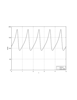
Рис. 1: Example 1. The expected number $E(X(t)|X(0))$ of customers in the queue for $t\in[0,5]$ with the initial condition $X(0)=0$.

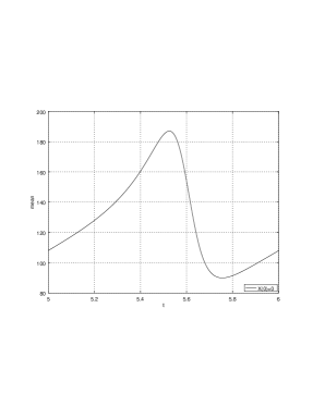
Рис. 2: Example 1. The expected number $E(X(t)|X(0))$ of customers in the queue for $t\in[5,6]$ with the initial condition $X(0)=0$.

Рис. 3: Example 1. The probability $p_{0}(t)$ of empty queue for $t\in[0,5]$ with the initial condition $X(0)=0$.

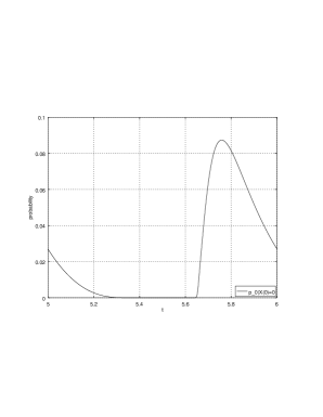
Рис. 4: Example 1. The probability $p_{0}(t)$ of empty queue for $t\in[5,6]$ with the initial condition $X(0)=0$.

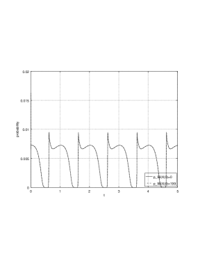
Рис. 5: Example 1. The probability $p_{99}(t)$ for $t\in[0,5]$ with the initial condition $X(0)=0$.

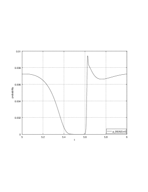
Рис. 6: Example 1. The probability $p_{99}(t)$ for $t\in[5,6]$ with the initial condition $X(0)=0$.

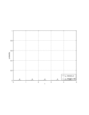
Рис. 7: Example 1. The probability $p_{199}(t)$ for $t\in[0,5]$ with the initial condition $X(0)=0$.

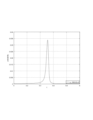
Рис. 8: Example 1. The probability $p_{199}(t)$ for $t\in[5,6]$ with the initial condition $X(0)=0$.

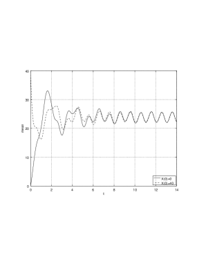
Рис. 9: Example 2. The expected number $E(X(t)|X(0))$ of customers in the queue for $t\in[0,14]$ with the initial conditions $X(0)=0$ and $X(0)=S$.

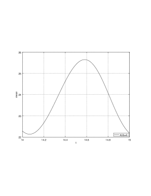
Рис. 10: Example 2. The expected number $E(X(t)|X(0))$ of customers in the queue for $t\in[14,15]$ with initial condition $X(0)=0$.

Рис. 11: Example 2. The probability $p_{0}(t)$ of empty queue for $t\in[0,14]$ with the initial conditions $X(0)=0$ and $X(0)=S$.

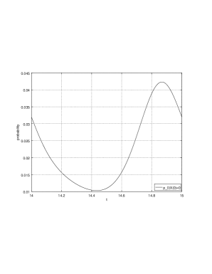
Рис. 12: Example 2. The probability $p_{0}(t)$ of empty queue for $t\in[14,15]$ with the initial condition $X(0)=0$.

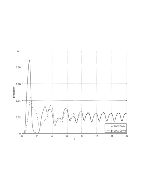
Рис. 13: Example 2. The probability $p_{20}(t)$ for $t\in[0,14]$ with the initial conditions $X(0)=0$ and $X(0)=S$.

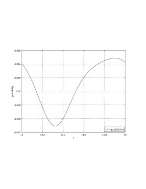
Рис. 14: Example 2. The probability $p_{20}(t)$ for $t\in[14,15]$ with the initial condition $X(0)=0$.

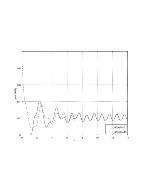
Рис. 15: Example 2. The probability $p_{40}(t)$ for $t\in[0,14]$ with the initial conditions $X(0)=0$ and $X(0)=S$.

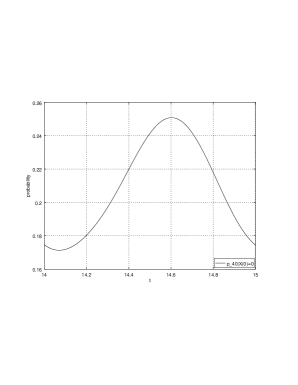
Рис. 16: Example 2. The probability $p_{40}(t)$ for $t\in[14,15]$ with the initial condition $X(0)=0$.

6 Conclusion

The three methods considered in this paper provide various alternatives for the computation of the upper bounds for the rate of convergence to the limiting regime of (in)homogeneous continuous-time Markov processes. Yet even for the four considered classes (i)–(iv) of Markov processes a single unified framework cannot be suggested: special cases do exist when none of the methods works well.

7 Acknowledgment

This research was supported by Russian Science Foundation under grant 19-11-00020.

• [1] B. Almasi. J. Roszik, J. Sztrik. Homogeneous finite-source retrial queues with server subject to breakdowns and repairs, Mathematical and Computer Modelling, 2005, 42, 673–682.
• [2] . A. Brugno, C. D Apice, A. Dudin, R. Manzo . Analysis of an $MAP/PH/1$ queue with flexible group service, International Journal of Applied Mathematics and Computer Science, 2017, 27, 119–131.
• [3] A. Di Crescenzo, V. Giorno, B. Krishna Kumar, A. Nobile. A Time-Non-Homogeneous Double-Ended Queue with Failures and Repairs and Its Continuous Approximation, Mathematics, 2018, 6:5, 81.
• [4] V. Giorno, A. Nobile, S. Spina. On some time non-homogeneous queueing systems with catastrophes, Applied Mathematics and Computation, 2014, 245, 220–234.
• [5] B. Granovsky, A. Zeifman. Nonstationary Queues: Estimation of the Rate of Convergence, Queueing Systems, 2004, 46, 363–388.
• [6] V. Kalashnikov. Analysis of ergodicity of queueing systems by Lyapunovś direct method, Automation and Remote Control, 1971, 32, 559–566.
• [7] N. Kartashov. Criteria for uniform ergodicity and strong stability of Markov chains with a common phase space, Theory of Probability and Mathematical Statistics, 1985, 30, 71–89.
• [8] J. Li, L. Zhang. $M^{X}/M/c$ Queue with catastrophes and state-dependent control at idle time, Frontiers of Mathematics in China, 2017, 12, 1427–1439.
• [9] H. Li, Q. Zhao, Z. Yang. Reliability Modeling of Fault Tolerant Control Systems, International Journal of Applied Mathematics and Computer Science, 2007, 17 ,491–504.
• [10] Y. Liu. Perturbation bounds for the stationary distributions of Markov chains, SIAM Journal on Matrix Analysis and Applications, 2012, 33, 1057–1074.
• [11] V. Malyshev, M. Menshikov. Ergodicity, continuity and analyticity of countable Markov chains, Transactions of the Moscow Mathematical Society, 1982, 1, 148.
• [12] S. Meyn, R. Tweedie. Stability of Markovian processes III: Foster-Lyapunov criteria for continuous time processes, Advances in Applied Probability, 1993, 25, 518–548.
• [13] S. Meyn, R. Tweedie. Markov chains and stochastic stability, Springer Science & Business Media, 2012.
• [14] A. Mitrophanov. Stability and exponential convergence of continuous-time Markov chains, Journal of Applied Probability, 2003, 40, 970–979.
• [15] A. Mitrophanov. The spectral gap and perturbation bounds for reversible continuous-time Markov chains, Journal of Applied Probability, 2004, 41, 1219–1222.
• [16] A. Mitrophanov. Connection between the rate of convergence to stationarity and stability to perturbations for stochastic and deterministic systems, 2018. Proceedings of the 38th International Conference Dynamics Days Europe, DDE 2018, Loughborough, UK. http://alexmitr.com/talk_DDE2018_Mitrophanov_FIN_post_sm.pdf
• [17] A. Moiseev, A. Nazarov. Queueing network ${MAP-(GI/\infty)K}$ with high-rate arrivals, European Journal of Operational Research, 2016, 254: 1, 161–168.
• [18] R. Nelson, D. Towsley, A. Tantawi. Performance Analysis of Parallel Processing Systems, IEEE Transactions on software engineering, 1988, 14: 4, 532–540.
• [19] T. Olwal, K. Djouani, O. Kogeda, B. Wyk. Joint queue-perturbed and weakly coupled power control for wireless backbone networks, International Journal of Applied Mathematics and Computer Science, 2012, 22, 749–764.
• [20] D. Rudolf, N. Schweizer. Perturbation theory for Markov chains via Wasserstein distance, Bernoulli, 2018, 24:4A, 2610–2639.
• [21] Y. Satin, A. Zeifman, A. Korotysheva, S. Shorgin. On a class of Markovian queues, Informatics and its Applications, 2011, 5: 4, 18–24.
• [22] Y. Satin, A. Zeifman, A. Korotysheva. On the Rate of Convergence and Truncations for a Class of Markovian Queueing Systems, Theory of Probability & Its Applications, 2013, 57, 529–539.
• [23] Ya. Satin, A. Zeifman, A. Kryukova .On the Rate of Convergence and Limiting Characteristics for a Nonstationary Queueing Model, Mathematics, 2019, 7, 678.
• [24] J. Schwarz, G. Selinka, R. Stolletz. Performance analysis of time-dependent queueing systems: Survey and classification, Omega, 2016, 63, 170–189.
• [25] K. K. Trejo, J. B. Clempner, A. S. Poznyak. Proximal constrained optimization approach with time penalization, Engineering Optimization, 2019, 51, 1207–1228.
• [26] E. Van Doorn, A. Zeifman, T. Panfilova. Bounds and asymptotics for the rate of convergence of birth-death processes, Theory of Probability and its Applications, 2010, 54, 97–113.
• [27] N. Vvedenskaya, A. Logachov, Y. Suhov, A. Yambartsev. A Local Large Deviation Principle for Inhomogeneous Birth-Death Processes, Problems of Information Transmission, 2018, 54:3, 263–280.
• [28] R. Wieczorek. Markov chain model of phytoplankton dynamics, International Journal of Applied Mathematics and Computer Science, 2010, 20, 763–771.
• [29] A. Zeifman. Stability for continuous-time nonhomogeneous Markov chains, Stability problems for stochastic models. Springer, Berlin, Heidelberg, 1985, 401–414.
• [30] A. Zeifman. Some properties of the loss system in the case of varying intensities. Automation and remote control, 1989, 50: 1, 107–113.
• [31] A. Zeifman. Upper and lower bounds on the rate of convergence for nonhomogeneous birth and death processes, Stochastic Processes and their Applications, 1995, 59, 157–173.
• [32] A. Zeifman, S. Leorato, E. Orsingher, Ya. Satin, G. Shilova. Some universal limits for nonhomogeneous birth and death processes, Queueing Systems, 2006, 52:2, 139–151.
• [33] A. Zeifmanm V. Korolev. On perturbation bounds for continuous-time Markov chains, Statistics & Probability Letters, 2014, 88, 66–72.
• [34] A. Zeifman, V. Korolev, Y. Satin, A. Korotysheva, V. Bening. Perturbation Bounds and Truncations for a Class of Markovian Queues, Queueing Systems, 2014, 76: 2, 205–221.
• [35] A. Zeifman, Y. Satin, V. Korolev, S. Shorgin. On truncations for weakly ergodic inhomogeneous birth and death processes, International Journal of Applied Mathematics and Computer Science, 2014, 24, 503–518.
• [36] A. Zeifman, V. Korolev. Two-sided bounds on the rate of convergence for continuous-time finite inhomogeneous Markov chains, Statistics & Probability Letters, 2015, 103, 30–36.
• [37] A. Zeifman, A. Korotysheva, V. Korolev, Y. Satin. Truncation Bounds for Approximations of Inhomogeneous Continuous-Time Markov Chains, Theory of Probability & Its Applications, 2017, 61, 513–520.
• [38] A. Zeifman, A. Sipin, V. Korolev, G. Shilova, K. Kiseleva, A. Korotysheva, Y. Satin. On Sharp Bounds on the Rate of Convergence for Finite Continuous-Time Markovian Queueing Models, Moreno-Diaz R., Pichler F., Quesada-Arencibia A. (eds). Computer Aided Systems Theory – EUROCAST 2017. EUROCAST 2017. Lecture Notes in Computer Science, 2018, 10672, 20–28.
• [39] A. Zeifman, R. Razumchik, Y. Satin, K. Kiseleva, A. Korotysheva, V. Korolev. Bounds on the Rate of Convergence for One Class of Inhomogeneous Markovian Queueing Models with Possible Batch Arrivals and Services, International Journal of Applied Mathematics and Computer Science, 2018, 28, 66–72.
• [40] A. Zeifman, V. Korolev, Y. Satin, K. Kiseleva. Lower bounds for the rate of convergence for continuous-time inhomogeneous Markov chains with a finite state space, Statistics & Probability Letters, 2018, 137 84–90.
• [41] A. Zeifman, K. Kiseleva, Y. Satin, A. Kryukova, V. Korolev. On a Method of Bounding the Rate of Convergence for Finite Markovian Queues, "10th International Congress on Ultra Modern Telecommunications and Control Systems and Workshops (ICUMT), Moscow, Russia 2018, 1–5.
• [42] A. Zeifman, Y. Satin, A. Kryukova. Applications of Differential Inequalities to Bounding the Rate of Convergence for Continuous-time Markov Chains, "AIP Conference Proceedings 2019, 2116, 090009.
• [43] Zeifman, A. I., Satin, Y. A., Kiseleva, K. M. On Obtaining Sharp Bounds of the Rate of Convergence for a Class of Continuous-Time Markov Chains. 2019, arXiv preprint arXiv:1905.10507.