Context-aware Active Multi-Step Reinforcement Learning

Abstract

Reinforcement learning has attracted great attention recently, especially policy gradient algorithms, which have been demonstrated on challenging decision making and control tasks. In this paper, we propose an active multi-step TD algorithm with adaptive stepsizes to learn actor and critic. Specifically, our model consists of two components: active stepsize learning and adaptive multi-step TD algorithm. Firstly, we divide the time horizon into chunks and actively select state and action inside each chunk. Then given the selected samples, we propose the adaptive multi-step TD, which generalizes TD($\lambda$), but adaptively switch on/off the backups from future returns of different steps. Particularly, the adaptive multi-step TD introduces a context-aware mechanism, here a binary classifier, which decides whether or not to turn on its future backups based on the context changes. Thus, our model is kind of combination of active learning and multi-step TD algorithm, which has the capacity for learning off-policy without the need of importance sampling. We evaluate our approach on both discrete and continuous space tasks in an off-policy setting respectively, and demonstrate competitive results compared to other reinforcement learning baselines.

1 Introduction

REINFORCE(Williams, 1992), as the most classic policy gradient approach (Sutton and Barto, 1998; Kakade, 2001; Schulman et al., 2015), directly optimizes the parameterized policy to improve the total return. The advantages of policy gradient algorithm is that it models the policy effectively by optimizing the parameters related to the policy control, and it handles high dimensional and continuous actions well. However, it suffers from high variance by delaying its model update and leading to slow learning until the end of the episode. Value-based (or critic only) approaches, such as Q-learning (Watkins and Dayan, 1992), iteratively improve its evaluations of the action-state pairs, which in turn can guide an agent what action to take under what circumstances. The updating procedure derived from Bellman equation needs to handle every state and action from environment, which is computationally intensive especially for the continuous action space. Actor-critic algorithms (Witten, 1977; Konda and Tsitsiklis, 1999) leverage both advantages of policy gradient and value function approaches(Sutton and Barto, 1998; Kakade, 2001; Schulman et al., 2015, 2017), such as lower variance and good convergence properties. Thus, actor-critic algorithms have gained popularity in reinforcement learning community recently. For example, Lillicrap et al. extends the actor-critic model using deep learning to handle the continuous action space (Lillicrap et al., 2015). Asynchronous Advantage Actor Critic ($A^{3}C$) (Mnih et al., 2016) presents a asynchronous version of actor critic algorithm, which uses parallel actor learners to update a shared model to make the learning process stabilized. Schulman et al. proposed a generalized advantage estimation (GAE) uses an exponentially-weighted estimator (Schulman et al., 2016) of the advantage function to reduce the variance of policy gradient. Recently, Twin Delayed Deep Deterministic Policy Gradients (TD3) (Fujimoto, van Hoof, and Meger, 2018) uses the minimum of two critics to limit the overestimated bias in actor-critic network. A soft actor critic algorithm (Haarnoja et al., 2018), an off policy actor-critic, leverages the maximum entropy to balance the exploration and exploitation in reinforcement learning framework. However, actor-critic as a special TD algorithm with one step (Sutton, 1988) updates the model (actor and critic) with every time step (Lillicrap et al., 2015; Haarnoja et al., 2018), which is time consuming and computationally intensive while updating a large deep model controller. Multi-step methods take a balance strategy between actor-critic ( or TD(0)) and Monte Carlo, and have gained resurgence in reinforcement learning (Asis et al., 2018; Hernandez-Garcia and Sutton, 2019), such as n-step Tree Backup (Precup, Sutton, and Singh, 2000), Retrace($\lambda$) (Munos et al., 2016), n-step Q($\sigma$) (Asis et al., 2018) and Sarsa (Rummery and Niranjan, 1994). Unfortunately, the step-size must be manually set up as the TD($\lambda$) (Sutton, 1988).

Instead of updating the model at each state, in this paper, we propose to actively learn the time step in the outer loop while internalizing the multi-step TD algorithm in the inner loop. However, it is a challenge to optimize the step size, considering the time step is a discrete variable. To do it, we divide the trajectories into intervals. Then, our method can select the most significant states and actions inside of each interval, which implicitly learns the step size in the outer loop. While in the inner loop, we propose the adaptive multi-step TD learning, which turns on/off the future backups if its context changes dramatically. In particular, we introudce a binary classifier for the future backups. Based on this function, our model generalizes TD($\lambda$) to adaptively detect the context change and take average of backups of different steps in the lookahead environment, and then update the model with the average target value to improve the training effectiveness.

In the experiments, we demonstrate that our active multi-step TD algorithm does in fact perform well by a wide margin on a bunch of continuous control tasks, compared to prior reinforcement learning methods.

2 Problem Setting and Notation

We consider the usual reinforcement learning problem (i.e. optimal policy existed) with sequential interactions between an agent and its environment (Sutton and Barto, 1998) in order to maximize a cumulative return. At every time step $t$, the agent selects an action $a_{t}$ in the state $s_{t}$ according its policy and receives a scalar reward $r_{t}(s_{t},a_{t})$, and then transit to the next state $s_{t+1}$. The problem is modeled as Markov decision process (MDP) with tuple: $(\mathcal{S},\mathcal{A},p(s_{0}),p(s_{t+1}|s_{t},a_{t}),r(s_{t},a_{t}),\gamma)$. Here, $\mathcal{S}$ and $\mathcal{A}$ indicate the state and action space respectively, $p(s_{0})$ is the initial state distribution. $p(s_{t+1}|s_{t},a_{t})$ is the state transition to $s_{t+1}$ given the current state $s_{t}$ and action $a_{t}$, $r(s_{t},a_{t})$ is reward from the environment after the agent taking action $a_{t}$ in state $s_{t}$ and $\gamma$ is the return discount factor, which is necessary to decay the future rewards ensuring bounded returns. We model the agent’s behavior with $\pi_{\theta}(a|s)$, which is a parametric distribution from a neural network.

Suppose we have the finite trajectory length while the agent interacting with the environment. The return under the policy $\pi$ for a trajectory $\tau={(s_{t},a_{t})}_{t=0}^{T}$

$$J(\theta) =E_{\tau\sim\pi_{\theta}(\tau)}[r(\tau)]=E_{\tau\sim\pi_{\theta}(\tau)}[R_{0}^{T}]$$

$$=E_{\tau\sim\pi_{\theta}(\tau)}[\sum_{t=0}^{T}\gamma^{t}r(s_{t},a_{t})]$$ (1)

where $\pi_{\theta}(\tau)$ denotes the distribution of trajectories,

$$\rho(\tau) =\pi(s_{0},a_{0},s_{1},...,s_{T},a_{T})$$

$$=p(s_{0})\prod_{t=0}^{T}\pi_{\theta}(a_{t}|s_{t})p(s_{t+1}|s_{t},a_{t})$$ (2)

For convenience, we can absorb $\gamma$ into reward in Eq. 2. The goal of reinforcement learning is to learn a policy $\pi$ which can maximize the expected returns.

$$\theta=\operatorname*{arg\,max}J(\theta)=\operatorname*{arg\,max}E_{\tau\sim\pi_{\theta}(\tau)}[R_{0}^{T}]$$ (3)

2.1 Policy gradient

Take the derivative w.r.t. $\theta$

$$\nabla_{\theta}J(\theta) =\nabla_{\theta}E_{\tau\sim\pi_{\theta}(\tau)}[R_{0}^{T}]=\nabla_{\theta}\int\rho(\tau)R_{0}^{T}d\tau$$

$$=\int\nabla_{\theta}\rho(\tau)R_{0}^{T}d\tau=\int\rho(\tau)\frac{\nabla_{\theta}\rho(\tau)}{\rho(\tau)}R_{0}^{T}d\tau$$

$$=E_{\tau\sim\pi_{\theta}(\tau)}[\nabla_{\theta}\textrm{log}\pi_{\theta}(\tau)R_{0}^{T}]$$ (4)

As we can see the high variance Eq. 2.1 is attributed to the stochastic rewards from trajectory. To reduce the variance, the baseline is introduced to Eq. 2.1. Then we have the following policy gradient:

$$\nabla_{\theta}J(\theta)=E_{\tau\sim\pi_{\theta}(\tau)}[\nabla_{\theta}\textrm{log}\pi_{\theta}(\tau)(R_{0}^{T}-b)]$$ (5)

If we replace the bias with value function $V(s)$, and factorize the above equation into each time step TD(0), we get

$$\nabla_{\theta}J(\theta)$$

$$= E_{\tau\sim\pi_{\theta}(\tau)}\bigg{[}\sum_{t=0}^{T}\nabla_{\theta}\textrm{log}\pi_{\theta}(a_{t}|s_{t})\big{(}Q(s_{t},a_{t})-V(s_{t})\big{)}\bigg{]}$$

$$= E_{\tau\sim\pi_{\theta}(\tau)}\bigg{[}\sum_{t=0}^{T}\nabla_{\theta}\textrm{log}\pi_{\theta}(a_{t}|s_{t})\big{(}r(s_{t},a_{t})+V(s_{t+1})-V(s_{t})\big{)}\bigg{]}$$ (6)

where $Q(s_{t},a_{t})=\sum_{t^{\prime}=t}^{T}E_{\pi_{\theta}}(r(s_{t},a_{t})|s_{t^{\prime}},a_{t^{\prime}})$, and $V(s_{t+1})=\sum_{{a_{t}}\sim\pi_{\theta}(\tau)}Q(s_{t},a_{t})$. In every time step $t$, the actor-critic algorithm updates parameters for the value function $V(s)$ with temporal difference and policy gradient in Eq. 2.1. This gradient has lower variance, i.e. single state transition, but is biased because of the potential inaccuracy of the lookahead estimate of $V(s)$. Thus, we can see that the bias-variance tradeoff is significantly influenced by the policy $\textrm{log}\pi_{\theta}(\tau)$ and the temporal difference $\delta_{t}(s_{t})$

$$\delta_{t}=\big{(}r_{t}+V(s_{t+1})\big{)}-V(s_{t})$$ (7)

Furthermore, given a specific time $t$, the contributions from $\pi_{\theta}(a_{t}|s_{t})$ and $\delta_{t}$ varies much to the policy gradient. For example, at some state $s_{t}$, if the temporal difference $\delta_{t}$ is too small, then we can skip this step to update actor-critic.

Instead of updating at each step $t$, we split the horizon into chunks, and find the most significant state (or $t$) inside each chunk, and then we query the oracle, such as actor-critic. In turn, we can update the model inside the actor-critic.

2.2 Value estimation

TD($\lambda$) is a popular TD learning algorithm (Sutton and Barto, 1998) to estimate state-value function $V(s_{t})$, which perfectly combines one-step TD prediction with Monte Carlo methods through the use of eligibility traces and the trace-decay parameter $\lambda$. Given the current policy $\pi_{\theta}$, the true value function $V(s_{t})$ at step $t$, which looks ahead to the end of episode with discounted rewards as

$$R_{t}^{T}=r_{t}+\gamma r_{t+1}+...+\gamma^{n}r_{t+n}+...$$ (8)

where $r_{t}$ is the reward at $s_{t}$ and $a_{t}$, which are omitted for simplicity. For $n$ step TD($n$), we can use $n$-step expected Sarsa to handle both on-policy and off-policy by using the return

$$R_{t}^{n}=r_{t}+\gamma r_{t+1}+...+\gamma^{n}E_{a\sim\pi(a)}(Q(s_{t+n},a_{t+n}))$$ (9)

Note that the first $n-1$ rewards are returns of states and actions sampled according to the behaviour policy, but the last state is backed up according to the expected action-value under the target policy. Similarily as TD($\lambda$), we can average $n$-step TD for different $n$ to balance the bias and variance. Suppose we get stepsize $n_{1},n_{2},...,n_{l}$, and look forward different timesteps ahead, then we can take the average and yield the return at time step $t$ as following

$$R_{t}^{avg}=\frac{\lambda_{1}R_{t}^{n_{1}}+\lambda_{2}R_{t}^{n_{2}}+...+\lambda_{l}R_{t}^{n_{l}}}{\lambda_{1}+\lambda_{2}+...+\lambda_{l}}$$ (10)

where $\lambda_{1},\lambda_{2},...,\lambda_{l}$ are the weights repectively for TD($n_{1}$), TD($n_{2}$),…, TD($n_{l}$).

One issue arising for multi-step reinforement learning is that we can’t assume that these trajectories would have been taken if the agent was using the current policy. In other words, we may need off-policy correction or importance sampling, which will reduce the impact of policies which are further away from the current one. However, the importance sampling has drawback with high variance, which can be compensated with small step sizes but it will slow learning (Precup, Sutton, and Singh, 2000). In the next section we present a method that unifies active learning to select states and actions, and adaptive TD$(\lambda)$ to switch on/off backups of different stepsizes.

3 Active multi-step TD learning

Our model consits of two pillars: active sample selection and adaptive multi-step TD learning. To speed up learning, we divide the time horizon into chunks and then select the most significant states. After we sample the states and actions, we propose an adaptive multi-step TD algorithm, which generalizes TD($\lambda$) by adaptively averaging backups of different $n$-step returns.

3.1 Active stepsize learning

For each trajectory $\tau=({s_{0},a_{0},s_{1},...,s_{T}})$ with length $T$, We split the horizon into chunks in Figure 1. Specifically, we can define a interval size $K$, which equally splits the horizon into $[T/K]$ chunks. Inside of each interval, we can actively select the most significant states to speed up learning. According to Eq. 2.1, we define the most significant state $(s_{t},a_{t})$ either has higher temporal difference or policy uncertainty. Note that we do not consider random policy in this paper. Thus, given the actor and critic, we select the most important time $t$, by maximizing the following objective in each interval $t\in[j,j+K]$:

$$\mathcal{L}(t;\theta)= \delta_{t}(s_{t})^{2}+\beta\textrm{H}\big{(}\textrm{log}\pi_{\theta}(a_{t}|s_{t})\big{)}$$ (11)

where $\textrm{H}\big{(}\textrm{log}\pi_{\theta}(a_{t}|s_{t})\big{)}$ is the entropy, $\delta_{t}$ is the one step temporal difference in Eq. 7 and $\beta$ is the weight to balance the above two terms.

For steps with higher $\delta_{t}$ and H($\cdot$) in Eq. 11, we should give them higher probability for exploration. So as in the active learning setting, we can always query actor-critic which step $t$ should be selected and further we can update our actor-critic models using TD learning. Specifically, if the current state $s_{t}$ has higher uncertain policy, it should query actor-critic to improve its policy at the current state. Similarly, if the current value approximator has higher bias, it should query actor-critic to update its value function. Our objective looks at the time step $t$ which has higher policy uncertainty (which leads to higher variance) and higher bias. Moreover, by selecting the most significant time $(s_{t},a_{t})$, we can explore the action space well to converge to the optimal policy while $K\to 1$ as TD(0). An example is shown in Fig. 2, where the red points are the steps selected by maximizing Eq. 11 inside each interval.

As for the discrete action space, we can take Eq. 11 to select the state-action inside the chunk, which can implictly adjust stepsize between successive states and then optimze the policy. In the continouse action space, we can use Gaussian policy in the $A^{2}C$. However, it performs poorly compared to DDPG (Lillicrap et al., 2015). Thus, we define another function for continous control below:

$$\mathcal{L}(t;\theta)=\delta_{t}(s_{t})^{2}+\beta(\nabla_{\theta}\textrm{log}\pi_{\theta}(a_{t}|s_{t}))^{2}$$ (12)

The difference between Eq. 11 and Eq. 12 is that the later uses policy gradient for the continous action space. The high value in Eq. 12, the high magnitude of gradient value in Eq. 2.1. In other words, we select the state-action pairs, which impacts the gradient most.

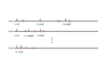
Figure 1: The coarse-to-fine actor-critic approach to select the state (or the time step).

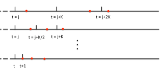
Figure 2: The active actor-critic approach to select the state (or the time step) inside the intervals.

Instead of updating actor-critic in every time step $t$, our strategy can select states inside intervals via active query to the current actor-critic architecture, which in turn implictly optimize the stepsize in the whole reinforcement learning framework. In the extreme case $K=1$, our model becomes the vanilla actor-critic method. Given the samples, we can use TD($n$) learning to update actor-critic model. Because we sample states, so the stepsize between successive states will be significant increased when $K>1$. One arising issue from TD($n$) learning may be the adverse effect from large $n$, which is even worse in continuous off-policy learning (Harutyunyan et al., 2016). This phenomenon has also been mentioned early in the Tree-backup algorithm (Precup, Sutton, and Singh, 2000).

In the following section, we introduce our adaptive multi-step TD learning, which can avoid correction or importance sampling in the large stepsize case.

3.2 Adaptive multi-step TD learning

Adaptive multi-step TD learning is a context-aware approach, which can decide whether to switch on or off future backups of different stepsizes. As mentioned before, given the interval length $K$, we can select the important states and actions based on Eq.12. Although the samples ($s_{t_{i}}$, $a_{t_{i}}$) at the different time $t_{i}$ is in order, the time difference ($t_{i+1}-t_{i}=1$) between occurrence of successive data points (which are actively sampled) does not hold anymore if $K>1$. Fortunately, we can still use the average multi-step TD($n$) via Eq. 10 over the sampled data $\{(s_{t_{i}},a_{t_{i}})\}$. Here, we introduce the binary variables which can adaptively decide whether to truncate the long term returns or not while averaging backups of different step lengths. If the state and action are not consistent, it may indicate there is significant context change, then we can turn off the long term returns, and only use the near term backups to update our model. On the contrary, if the long term state and action is consisitent with the current environment, we can include it in our value estimation.

The motivation we introduce the binary variables to TD$(\lambda)$ is to reduce its variance. In the early stage of learning, $n$-step bootstrapping with large $n$ (as $n\to T$, it equals to the Monte Carlo return) can better fit the true value function. As the value function is better estimated, it is will be better if we can reduce its variance in the late stage of learning. Recall that:

$$R_{t}^{n}=r_{t}+\gamma r_{t+1}+...+\gamma r_{t+n-1}+\gamma^{n}V(s_{t+n})$$ (13)

Then we can compute the variance of $R_{t}^{n}$ as: $\displaystyle Var(R_{t}^{n})=$ $\displaystyle Var[R_{t}^{n-1}-\gamma^{n-1}V(s_{t+n-1})+\gamma^{n-1}r_{t+n-1}+\gamma^{n}V(s_{t+n})]$ $\displaystyle=$ $\displaystyle Var[R_{t}^{n-1}-\gamma^{n-1}(r_{t+n-1}+V(s_{t+n})-V(s_{t+n-1}))]$ $\displaystyle=$ $\displaystyle Var[R_{t}^{n-1}]+\gamma^{2(n-1)}Var((r_{t+n-1}+V(s_{t+n})-V(s_{t+n-1})))$ $\displaystyle+2Cov(R_{t}^{n-1},(r_{t+n-1}+V(s_{t+n})-V(s_{t+n-1})))$ $\displaystyle\approx$ $\displaystyle Var[R_{t}^{n-1}]+\gamma^{2(n-1)}Var((r_{t+n-1}+V(s_{t+n})-V(s_{t+n-1})))$ $\displaystyle=$ $\displaystyle Var[R_{t}^{n-1}]+\gamma^{2(n-1)}Var(\delta_{t}(n))$ (14)

where we assume $Cov(R_{t}^{n},R_{t}^{n-1})\approx Var(R_{t}^{n-1})$ considering the highly correlation between $R_{t}^{n}$ and $R_{t}^{n-1}$ in successive sequences. So that we have $Cov(R_{t}^{n-1},(r_{t+n-1}+V(s_{t+n})-V(s_{t+n-1})))\approx 0$ as in (Kearns and Singh, 2000). As $n$ increasing, the variance of the $n$-step return $R_{t}^{n}$ increases correspondingly, which is contributed from $Var(\delta_{t}(n))$. In addition, $\delta_{t}(n)$ can be thought as the advantage over the current state. If its sign changes, it may lead to high variance. Thus, if $Var(\delta_{t}(n))$ changes rapidly, we can truncate the future backups to reduce the variance of TD$(\lambda)$.

Hence, we extend Eq. 10 by introducing binary variables to turn on or off different steps while we compute the average return at $t_{i}$

$$R_{t_{i}}^{avg}=\frac{\lambda_{1}b_{1}R_{t_{i}}^{n_{1}}+\lambda_{2}b_{2}R_{t_{i}}^{n_{2}}+...+\lambda_{l}b_{l}R_{t_{i}}^{n_{l}}}{\lambda_{1}b_{1}+\lambda_{2}b_{2}+...+\lambda_{l}b_{l}}$$ (15)

where $R_{t_{i}}^{n_{l}}$ is defined via Eq. 9, and $b_{i},i=\{1,2,...,l\}$ is the context-aware binary variable, which will be learned based on the consisitency between states and actions. If ${b_{l}=0}$, then its branch backup from $R_{t_{i}}^{n_{l}}$ will be turned off. Otherwise, it will include $R_{t_{i}}^{n_{l}}$ in the average of backups above.

In our model, we train a binary classifier $f(s,a)$ to model context change. Especially, given $(s_{t_{i}},a_{t_{i}})$, we use the sign of the advantage $Q(s_{t_{i}},a_{t_{i}})-V(s_{t_{i}})$ as the groundtruth, then we can learn a binary classifier $y=f(s,a)$. So for the future environment $(s_{n_{l}},a_{n_{l}})$, we define $b_{l}$ as follows

$$b_{l}=[f(s_{t_{i}},a_{t_{i}})==f(s_{n_{l}},a_{n_{l}})]$$ (16)

The purpose we introduce $b_{l}$ for TD($n_{l}$) is to capture the context consistence while we average the different stepsize returns. So our model is a context-aware approach, which can automatically turn on/off certain backups if it detects significantly environmental changes. In addition, we can add more information, such as stepsize and action difference, to the context except states and actions while learning the binary classifier.

3.3 Algorithms

Assume that we have $N$ trajectories ${\{\tau_{i}\}_{i=1}^{N}}$, where $\tau_{i}=({s_{0},a_{0},s_{1},...,s_{T_{i}}})$. Further, we define a list of $M$ intervals $\mathcal{K}=\{K_{1},K_{2},...,K_{M}\}$, where each $K_{m}$ specifies the interval size. If we take a coarse to fine scale in the horizon, then intervals satisfy $T>K_{1}\geq...\geq K_{M}=1$, shown in Fig. 1. Moreover, the step distance between samples in successive intervals will vary from time to time, shown in Fig. 2. On the contrary, we can also take a fine to coarse approach, by setting $1\leq K_{1}\leq...\leq K_{M}<T$. Of course, we can set a fixed $K_{m}$ for any $m$ over all these trajectories. Note that $K_{m}$ for $m\in[1,M]$ can be any integer as long as $K_{i}\in[1,T]$. In addition, we can calculate the number of trajectories $N_{i}$ assigned to each interval, where $N_{i}=[N/M]$ if the trajectories are equally distributed over the total $M$ intervals. Our active multi-step TD in Algorithm 1 comprises two loops: the loop for state selection and the loop to update actor-critic model using adpative multi-step TD learning. In the active selection stage, we do the inference over the steps $t\in[j,j+K]$, where $K\in\mathcal{K}$, and select $(s_{t},a_{t})$ by maximizing Eq. 12. In the learning stage, we can consider two situatioins: on-policy and off-policy learning. In the on-policy case, we can immediately update the model with TD(0). As for the off-policy, we can put the sampled data into buffer, and then we can update actor-critic with adpative multi-step TD by sampling the data from the buffer. Note that we can use any state of the art TD algorithm in our context-aware framework to improve the performance. Note that $r_{t}$ in Algorithm 1 is the accumulated reward over the past steps under the behavior policy.

Algorithm 1 Active multi-step TD algorithm

  Initialize critic network $Q(s,a|\theta^{Q})$ and actor $\mu(s|\theta^{\mu})$ with weights $\theta^{Q}$ and $\theta^{\mu}$

  Initialize the binary classifier $f(s,a)$

  Initialize $M$ intervals $[K_{1},K_{2},...,K_{M}]$

  Initialize the total number of episodes $N$ and the replay buffer R

  Initialize the coefficient $\beta$ in Eq. 12

  Initialize the number of lookahead backups $l$

  Calculate the number of episodes for each interval $[N/M]$

  for episode = 1 to $N$ do

     Compute the interval size $K=K_{episode\%M}$

     $D$ = [ ] // samples from the trajectory

     Receive initial observation state $s_{0}$ from the environment

     for $t=0$ to $T$ do

        Select action according to $a_{t}=\mu(s_{t}|\theta^{\mu})$

        Execute action $a_{t}$ and receive reward $r_{t}$, $done$, and further observe new state $s_{t+1}$

        Compute the selection function $\mathcal{L}(t;\theta)$ in Eq. 12

        if $t\%K==0$ then

           Select the most significant state $(s_{t},a_{t})$

           Add the sample $(s_{t},a_{t},r_{t},t,s_{t+1})$ into $D$

        end if

     end for

     for  $t$ =1 to length($D$)  do

        Push continuous $l$ tuples of $(s_{t},a_{t},r_{t},t,s_{t+1})$ into R

     end for

     Update the actor and critic via Algorithm 2

  end for

  Return parameters $\theta=\{\theta^{Q},\theta^{\mu}\}$.

Algorithm 2 Adaptive multi-step TD algorithm

  Input: critic network $Q(s,a|\theta^{Q})$ and actor $\mu(s|\theta^{\mu})$, and their target networks

  Input: the binary classifier $f(s,a)$

  Input: the number of lookahead backups $l$

  Input: the number of iterations $Iter$

  Input: the batchsize

  for i = 1 to $Iter$ do

     Sample a batchsize of $l$ continuous tuples from R: $(s_{t_{i}},a_{t_{i}},r_{t_{i}},t_{i},s_{t_{i}+1})$, …, $(s_{t_{i}+n_{l}},a_{t_{i}+n_{l}},r_{t_{i}+n_{l}},t_{{i}+l},s_{t_{i}+n_{l}})$

     Infer the binary variables $b_{1}$, …, $b_{l}$ via $f(s,a)$

     Compute the average return at ${t_{i}}$ via Eq. 15

     Compute the advantage and its sign $y_{t_{i}}$,

     Prepare the training data $\{(s_{t_{i}},a_{t_{i}}),y_{t_{i}}\}$

     Update critic $Q(s,a|\theta^{Q})$

     Update actor $\mu(s|\theta^{\mu})$

     Update target networks

     Update the classifier $f(s,a)$ with $\{(s_{t_{i}},a_{t_{i}}),y_{t_{i}}\}$

  end for

  Return parameters $\theta=\{\theta^{Q},\theta^{\mu}\}$ and the classifier $f(s,a)$.

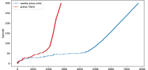
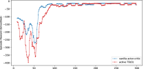
(a)	(b)	(c)

Figure 3: The results on the Cliff Walking problem. (a) and (b) show how many episodes are required to reach the maximum return, which demonstrates that our method with active selection can use the training data more effectively. (c) indicates how the smoothed (window size 10) reward changes while increasing the number of episodes in the learning process. Our active TD shows much stable results with more episodes.

4 Experiments

In this section, we evaluate our method on both descrete and continous action space. In particular, we test whether the active selection works or not without including the context-aware strategy. In addition, we also combines both active learning and off-policy adaptive multi-step TD in algoirthm 1 to verify whether the context-aware strategy contributes to boost the overall return.

In the descrete action space, we mainly test whether the active selection contributes or not in our active TD algorithm. We use a simple TD(0) learning with actor and critic networks, and sample the action based on the actor network. The deep achitecture for both actor and critic uses a hidden layer with 20 dimensions. The batch size is set 100, learning rate is 0.001 for actor and 0.01 for critic respectively, and $\beta=0.1$. While we update actor and critic, namely TD(0), we do not consider returns of different stepsizes. So we set $K_{m}=1$ for all $m\in[1,M]$ and $l=1$ in Eq. 15, referring Algorithm 2 for more details. Both target networks are updated with $\tau=0.001$ if not specified. We compared our approach with other baselines, such as active-critic, REINFORCE and DQN.

The result on cliff walking environment is shown in Figure 3. Compared to vanilla actor-critic, our model can leverage the episodes more efficiently and achieve optimal state with short steps, shown in Figure 3(a). In addition, we test our approach on another three classical environments, and the learning curves shown in Figure 4 indicate our approach matches or outperform the other three baselines. Fig. 4(a) shows the comparison on Cartpole enviroment. Our simple active TD(0) has better average return, compared to other methods. Similar result is observed in MoutainCar environment. In the Acrobot enviroment, vanilla actor-critic is better at the beginning episode. But our method yield much better and stable returns in the late episodes.

In the continous action space, we mainly test adaptive multi-step TD with the interval size $K_{m}=4$ fixed for all $m\in[1,M]$ and measure its performance on a suite of different control tasks. Without other specification, we use the same parameters below for all environments. The deep achitecture for both actor and critic uses the same networks as TD3 (Fujimoto, van Hoof, and Meger, 2018), with hidden layers [400, 300, 300]. Note that the actor adds the noise $\mathcal{N}(0,0.1)$ to its action space to enhance exploration and the critic network has two Q-functions as TD3. In addition, we also use target networks (for both actor and critic) to improve the performance as in DDPG and TD3. The target policy is smoothed by adding Gaussian noise $\mathcal{N}(0,0.2)$ as in TD3. The classifier uses the same network structure as critic, but with binary (softmax) output. The number of lookaheads $l=3$ to incorporate different backups. For $n_{1}$, we use the minimum of the dual Q-function as TD3 to get the target value, while for $n_{2}$ and $n_{3}$, we use the average of the dual Q-value in Eq. 9. The weights $\lambda_{i}$ over TD($n_{i}$) for $i=\{1,2,3\}$ decay exponentially with the base $\frac{1}{2}$ as in TD($\lambda$). Both target networks are updated with $\tau=0.005$. In addtion, the off-policy algorithm uses the replay buffer with size $10^{6}$ for all experiments as TD3 did.

The earning curves with exploration noise are shown in Figures 5 and 6. It demonstrates that our approach can yield competitive results, compared to TD3 and DDPG. Specifically, our active multi-step TD approach outperforms all other algorithms on HalfCheetah, Walker2d and BipedalWalker in both final performance and learning speed across all tasks. The quatitative results over 5 trials are presented in Table 1. Except Reacher and BipedalWalker, we learn the model until to 1 million samples and then evaluate the reward. We repeat this with 5 trials and then we can calcualte the average return. For Reacher task, it converges fast, so we only sample 100k steps. Similarly, we use 350k samples in BipedalWalker environment. It shows that our approach yields significantly better results on HalfCheetah, Walker2d and BipedalWalker. Note that we only try the fix interval size $K_{m}=4$. By varying the interval size, our approach can easily yield comparable or even better results on the other three MuJoCo environments.

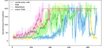
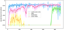
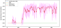
(a) Cartpole	(b) Acrobot	(c) MoutainCar

Figure 4: The result (smoothed over window size 10) on the Cartpole, Acrobot and MoutainCar environments. It demonstrates that our active sample selection can boost performance.

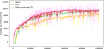
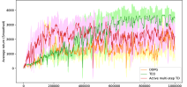
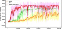
(a) Halfcheetah	(b) Hopper	(c) Walker2d

Figure 5: The Learning curves with exploration noise on the Halfcheetah, Hopper and Walker2d environments. The shaded region represents the standard deviation of the average evaluation over nearby windows with size 10. Our active multi-step TD algorithm yields significantly better results, compared to TD3 and DDPG.

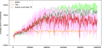
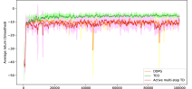
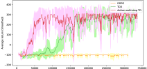
(a) Ant	(b) Reacher	(c) BipedalWalker

Figure 6: Learning curves for the OpenAI gym continuous control tasks with exploration noise. The shaded region represents the standard deviation of the average evaluation over nearby windows with size 10. It shows that our approch on BipedalWalker can more effeciently use the training samples and yield higher returns.

Methods	Environments
	HalfCheetah	Hopper	Walker2d	Ant	Reacher	InvPendulum	BipedalWalker
DDPG	8577.29	2020.46	1843.85	1005.30	-6.51	1000	$-101.40\pm 0.4$
TD3	$9636.95\pm 859.06$	$\bf{3564.07\pm 114.74}$	$4682.82\pm 539.64$	$\bf{4373.44\pm 1000.33}$	$\bf{-3.6\pm 0.56}$	$1000\pm 0.0$	$255.6\pm 74.2$
Active Multi-step TD	$\bf{9836.5\pm 611.10}$	$3063.05\pm 357.21$	$\bf{5092.57\pm 270.71}$	$3135.67\pm 325.86$	$-10.21\pm-1.64$	$\bf{1000\pm 0.0}$	$\bf{275.03\pm 98.1}$

Table 1: Comparison of Max Average Return over 5 trials of 1 million samples, except Reacher and BipedalWalker. The maximum value is marked bold for each task. $\pm$ corresponds to a single standard deviation over trials. Note that we only try the interval size equal to 4 in this experiment.

5 Related work

Our active multi-step TD algorithm incorporates two key ingredients: active learning with objective which consists of TD errors and entropy maximization to enable stability and exploration, coarse-to-fine time chunking, and multi-step TD learning with an actor-critic architecture. In this section, we review previous works that draw on some of these topics.

The basic idea of actor-critic algorithms (Witten, 1977; Konda and Tsitsiklis, 1999) is that it learns the policy and value function simultaneously, where the actor takes action according to the current policy while the critic (or value function) estimates whether this action will improve the total returns or not. Further, the advantage actor-critic ($A^{2}C$) introduces the average value to each state, and leverages the difference between value function and the average to update the policy parameters. In other words, the good policy which leads to high value function will be enhanced and bad policy will be suppressed. Since the policy updates in each time step (or state), it can significantly reduce the variance compared to REINFORCE.

How to balance the variance and bias is an interesting topic in the reinforcement learning. $TD(\lambda)$ (Sutton, 1988) was first introduced by Sutton to update value function and learn policy control. The coefficient $\lambda\in[0,1]$ trades off between bias and variance, and empirically shows that intermediate $\lambda$ performs best. For each state on the trajectory, $TD(\lambda)$ adjusts the parameter $\lambda$ to approximate target value function, where $\lambda=1$ is the Monte-Carlo return, i.e. sum of discounted future rewards. This is unbiased, but may have high variance because of the long stochastic sequence of rewards. For $\lambda=0$, the target value is updated using Bellman equation by sampled one-step lookahead. Unfortunately, this value may be biased because of the potential inaccurate estimation of value function. Apparently, it is a challenge to achieve the good balance between bias and variance, because it requires the user to tune a stepsize manually. Late, it was extended with least squares TD in (Bradtke, Barto, and Kaelbling, 1996; Boyan, 2002) to approximate the value function by summing the decayed estimators, in order to eliminate all stepsize parameters and improve data efficiency. Recently, Schulman et al. proposed a similar method, called the generalized advantage value estimation (Schulman et al., 2016), which considered the whole episode with an exponentially-weighted estimator of the advantage function that is analogous to $TD(\lambda)$ to substantially reduce bias of policy gradient estimates. However, the actor-critic methods provides the low-variance baseline at the cost of the some bias and remain sample inefficient. Moreover, the actor-critic updates policy and value function at “arbitrarily” every state, which slows down the whole training process especially for the deep network approximators.

Another trend is to combine maximum entropy with policy gradient in reinforcement learning to balance exploration and exploitation. Maximum entropy inverse reinforcement learning (Ziebart et al., 2008) was proposed to maximize the likelihood of the observed data with maximum entropy constraint. Relative Entropy Policy Search (Peters, Mülling, and Altün, 2010) extends policy gradient under the relative entropy constraints, such as Kullback-Leibler divergence. Haarnoja et al. proposed soft Q-learning (Haarnoja et al., 2017), by incorporating maximum entropy into policy control, and showed it improved exploration and compositionality. Late, soft Q-learning is extend to soft actor critic (Haarnoja et al., 2018), an off-policy algorithm based on the maximum entropy, where the actor aims to maximize expected reward while also maximizing entropy.

Active learning has also been applied on reinforcement learning. For example, active inverse reinforcement learning (Lopes, Melo, and Montesano, 2009) was proposed that allows the agent to query the demonstrator for samples at specific states, instead of relying only on samples provided at “arbitrary” states. Active Reinforcement Learning (Epshteyn, Vogel, and DeJong, 2008) is another method, which focuses on how policy is affected by changes in transition probabilities and rewards of individual actions, and then determine which states are worth exploring based solely on the prior MDP specification. Compared to previous active reinforcement learning (Epshteyn, Vogel, and DeJong, 2008), our approach focuses on adaptively learning the step-size, while former method relies on the sensitivity of the optimal policy to the transitions and rewards. Riad et al. proposed APRIL (Akrour, Schoenauer, and Sebag, 2012), an active ranking mechanism, which combined with preference-based reinforcement learning in order to decrease the number of ranking queries to the expert needed to yield a satisfactory policy. Our approach takes a more similar strategy as (Lopes, Melo, and Montesano, 2009) to query critic-critic and select the most significant states and steps to update the actor-critic in the inner loop. In a sense, it is more related to the meta-learning (Finn, Abbeel, and Levine, 2017; Al-Shedivat et al., 2018; Xu, van Hasselt, and Silver, 2018).

For example, meta-policy gradient algorithm in (Xu et al., 2018) adaptively learns a global exploration policy in deep deterministic policy gradient (Lillicrap et al., 2015) to speed up the learning process significantly. Meta-gradient reinforcement learning in (Xu, van Hasselt, and Silver, 2018) takes gradients w.r.t. the meta-parameters (such as discount factor or bootstrapping parameter) of a return function. Our meta-learning approach learns the step size to improve sample efficiency and stabilize and speed up the learning process. But stepsize is discrete variable, which is hard to optimize use the prior gradient-based algorithm. Moreover, the step size should be adaptively changed to reflect the importance of states in the horizon. In this paper, we leverage active learning to query actor-critic and adaptively select the states and steps, which in turn are feedback to actor-critic to learn better policy and value function.

6 Conclusion

In this paper, we propose a context-aware multi-step reinforcement learning method, which can actively select states and actions, and switch on/off future backups adaptively while updating model parameters based on the context change. Specifically, we introduce the intervals or chunks to actively select states and adaptive multi-step TD with a context-aware classifier to turn on/off future rewards while computing the target value. The adaptive multi-step TD can leverage the recent TD algorithms such as TD3, and moreover it generalized TD($\lambda$) to adaptively average different n-step returns with corresponding binary variables. Furthermore, our approach internalizes multi-step TD learning, and can leverage any advanced reinforcement learning models to improve performance. The experimental results demonstrate our approach is effective on off-policy tasks, especially in the continuous control setting.

References

- Akrour, Schoenauer, and Sebag (2012) Akrour, R.; Schoenauer, M.; and Sebag, M. 2012. April: Active preference learning-based reinforcement learning. In Proceedings of the 2012th European Conference on Machine Learning and Knowledge Discovery in Databases - Volume Part II, ECMLPKDD’12, 116–131. Berlin, Heidelberg: Springer-Verlag.
- Al-Shedivat et al. (2018) Al-Shedivat, M.; Bansal, T.; Burda, Y.; Sutskever, I.; Mordatch, I.; and Abbeel, P. 2018. Continuous adaptation via meta-learning in nonstationary and competitive environments. In ICLR.
- Asis et al. (2018) Asis, K. D.; Hernandez-Garcia, J. F.; Holland, G. Z.; and Sutton, R. S. 2018. Multi-step reinforcement learning: A unifying algorithm. In AAAI, 2902–2909. AAAI Press.
- Boyan (2002) Boyan, J. A. 2002. Technical update: Least-squares temporal difference learning. In Machine Learning, 233–246.
- Bradtke, Barto, and Kaelbling (1996) Bradtke, S. J.; Barto, A. G.; and Kaelbling, P. 1996. Linear least-squares algorithms for temporal difference learning. In Machine Learning, 22–33.
- Epshteyn, Vogel, and DeJong (2008) Epshteyn, A.; Vogel, A.; and DeJong, G. 2008. Active reinforcement learning. In Proceedings of the 25th International Conference on Machine Learning, 296–303. New York, NY, USA: ACM.
- Finn, Abbeel, and Levine (2017) Finn, C.; Abbeel, P.; and Levine, S. 2017. Model-agnostic meta-learning for fast adaptation of deep networks. In ICML, volume 70 of Proceedings of Machine Learning Research, 1126–1135. PMLR.
- Fujimoto, van Hoof, and Meger (2018) Fujimoto, S.; van Hoof, H.; and Meger, D. 2018. Addressing function approximation error in actor-critic methods. In ICML, volume 80 of JMLR Workshop and Conference Proceedings, 1582–1591. JMLR.org.
- Haarnoja et al. (2017) Haarnoja, T.; Tang, H.; Abbeel, P.; and Levine, S. 2017. Reinforcement learning with deep energy-based policies. In ICML, volume 70 of Proceedings of Machine Learning Research, 1352–1361. PMLR.
- Haarnoja et al. (2018) Haarnoja, T.; Zhou, A.; Abbeel, P.; and Levine, S. 2018. Soft actor-critic: Off-policy maximum entropy deep reinforcement learning with a stochastic actor. In ICML, volume 80 of JMLR Workshop and Conference Proceedings, 1856–1865. JMLR.org.
- Harutyunyan et al. (2016) Harutyunyan, A.; Bellemare, M. G.; Stepleton, T.; and Munos, R. 2016. Q() with off-policy corrections. In ALT.
- Hernandez-Garcia and Sutton (2019) Hernandez-Garcia, J. F., and Sutton, R. S. 2019. Understanding multi-step deep reinforcement learning: A systematic study of the DQN target. CoRR abs/1901.07510.
- Kakade (2001) Kakade, S. 2001. A natural policy gradient. In Proceedings of the 14th International Conference on Neural Information Processing Systems: Natural and Synthetic, NIPS’01, 1531–1538. Cambridge, MA, USA: MIT Press.
- Kearns and Singh (2000) Kearns, M. J., and Singh, S. P. 2000. Bias-variance error bounds for temporal difference updates. In Proceedings of the Thirteenth Annual Conference on Computational Learning Theory, COLT ’00, 142–147. San Francisco, CA, USA: Morgan Kaufmann Publishers Inc.
- Konda and Tsitsiklis (1999) Konda, V. R., and Tsitsiklis, J. N. 1999. Actor-critic algorithms. In Advances in Neural Information Processing Systems, 1008–1014. MIT Press.
- Lillicrap et al. (2015) Lillicrap, T. P.; Hunt, J. J.; Pritzel, A.; Heess, N.; Erez, T.; Tassa, Y.; Silver, D.; and Wierstra, D. 2015. Continuous control with deep reinforcement learning. CoRR abs/1509.02971.
- Lopes, Melo, and Montesano (2009) Lopes, M.; Melo, F. S.; and Montesano, L. 2009. Active learning for reward estimation in inverse reinforcement learning. In European Conference on Machine Learning (ECML/PKDD).
- Mnih et al. (2016) Mnih, V.; Badia, A. P.; Mirza, M.; Graves, A.; Harley, T.; Lillicrap, T. P.; Silver, D.; and Kavukcuoglu, K. 2016. Asynchronous methods for deep reinforcement learning. In Proceedings of the 33rd International Conference on International Conference on Machine Learning - Volume 48, ICML’16, 1928–1937. JMLR.org.
- Munos et al. (2016) Munos, R.; Stepleton, T.; Harutyunyan, A.; and Bellemare, M. G. 2016. Safe and efficient off-policy reinforcement learning. In NIPS, 1046–1054.
- Peters, Mülling, and Altün (2010) Peters, J.; Mülling, K.; and Altün, Y. 2010. Relative entropy policy search. In Proceedings of the Twenty-Fourth AAAI Conference on Artificial Intelligence, AAAI’10, 1607–1612. AAAI Press.
- Precup, Sutton, and Singh (2000) Precup, D.; Sutton, R. S.; and Singh, S. P. 2000. Eligibility traces for off-policy policy evaluation. In ICML, 759–766. Morgan Kaufmann.
- Rummery and Niranjan (1994) Rummery, G. A., and Niranjan, M. 1994. On-line q-learning using connectionist systems. Technical report.
- Schulman et al. (2015) Schulman, J.; Levine, S.; Moritz, P.; Jordan, M.; and Abbeel, P. 2015. Trust region policy optimization. In Proceedings of the 32Nd International Conference on International Conference on Machine Learning - Volume 37, ICML’15, 1889–1897. JMLR.org.
- Schulman et al. (2016) Schulman, J.; Moritz, P.; Levine, S.; Jordan, M.; and Abbeel, P. 2016. High-dimensional continuous control using generalized advantage estimation. In Proceedings of the International Conference on Learning Representations (ICLR).
- Schulman et al. (2017) Schulman, J.; Wolski, F.; Dhariwal, P.; Radford, A.; and Klimov, O. 2017. Proximal policy optimization algorithms. CoRR abs/1707.06347.
- Sutton and Barto (1998) Sutton, R. S., and Barto, A. G. 1998. Reinforcement learning - an introduction. Adaptive computation and machine learning. MIT Press.
- Sutton (1988) Sutton, R. S. 1988. Learning to predict by the methods of temporal differences. Mach. Learn. 9–44.
- Watkins and Dayan (1992) Watkins, C. J. C. H., and Dayan, P. 1992. Q-learning. In Machine Learning, 279–292.
- Williams (1992) Williams, R. J. 1992. Simple statistical gradient-following algorithms for connectionist reinforcement learning. In Machine Learning, 229–256.
- Witten (1977) Witten, I. H. 1977. An adaptive optimal controller for discrete-time markov environments. Information and Control 286–295.
- Xu et al. (2018) Xu, T.; Liu, Q.; Zhao, L.; and Peng, J. 2018. Learning to explore via meta-policy gradient. In Proceedings of the 35th International Conference on Machine Learning, 5463–5472.
- Xu, van Hasselt, and Silver (2018) Xu, Z.; van Hasselt, H.; and Silver, D. 2018. Meta-gradient reinforcement learning. In CoRR, volume abs/1805.09801.
- Ziebart et al. (2008) Ziebart, B. D.; Maas, A.; Bagnell, J. A.; and Dey, A. K. 2008. Maximum entropy inverse reinforcement learning. In Proceedings of the 23rd National Conference on Artificial Intelligence - Volume 3, 1433–1438. AAAI Press.