Linear-Quadratic Time-Inconsistent Mean-Field Type Stackelberg Differential Games: Time-Consistent Open-Loop Solutions

Abstract

In this paper, we consider the linear-quadratic time-inconsistent mean-field leader-follower Stackelberg stochastic differential game with an adapted open-loop information structure. Given a controlled linear stochastic differential equation (SDE), the quadratic objective functionals of the leader and the follower include conditional expectations of state and control (mean field) variables. In addition, the cost parameters could be general nonexponential discounting depending on the initial time. As stated in the existing literature, these two general settings of the objective functionals induce time inconsistency in the optimal solutions. Given an arbitrary control of the leader, we first obtain the follower’s (time-consistent) equilibrium control and its state feedback representation in terms of the nonsymmetric coupled Riccati differential equations (RDEs) and the backward SDE. This provides the rational behavior of the follower, characterized by the forward-backward SDE (FBSDE). We then obtain the leader’s explicit (time-consistent) equilibrium control and its state feedback representation in terms of the nonsymmetric coupled RDEs, where the constraint of the leader’s problem is the FBSDE induced by the follower’s rational behavior. With the solvability of the nonsymmetric coupled RDEs, the equilibrium controls of the leader and the follower constitute the time-consistent Stackelberg equilibrium of the paper. Finally, the numerical examples are provided to check the solvability of the nonsymmetric coupled RDEs of the leader and the follower.

I Introduction

One of the most important features of (deterministic and stochastic) optimal control that is typically not emphasized is time consistency, which states that the optimal solution obtained with respect to the initial time $t\in[0,T]$ and the initial state $x(t)=x$ (equivalently the initial pair $(t,x)$) remains optimal when it is restricted on $[\tau,T]$ with the initial condition $x(\tau)$ (equivalently the initial pair $(\tau,x(\tau))$ with $\tau\in(t,T]$ [1, 2, 3, 4]. The time-consistent property stems from Bellman’s principle of optimality (dynamic programming), which formulates the optimal control problem as a family of the initial pair $(t,x)$. In fact, the dynamic programming approach provides a theoretical foundation for optimal control theory (and differential games) by characterizing the value function in terms of the initial pair $(t,x)$, which leads to the Hamilton-Jacobi-Bellman (HJB) equation [5, 6, 7].

We expect that all (deterministic and stochastic) optimal control problems hold the time-consistent property. However, in many situations, the time-consistency fails. Specifically, as discussed in the examples of [3, Examples 1.1 and 1.2], [8, Section 2] and [9, 4], this is due to the fact that

1. the cost parameters in the objective functional could be general nonexponential discounting parameters that are dependent on the initial time;

2. the conditional expectations of state and control variables could be included in the state equation (e.g. stochastic differential equation, SDE) and the objective functional.

Under the above two general settings, time-inconsistent (deterministic and stochastic) optimal control problems can be formulated. Regarding (1), in [10, 11, 12, 13, 14, 15, 16, 17, 18, 19], time-inconsistent (deterministic and stochastic) optimal control problems with general (nonexponential) discounting parameters including quasi-exponential discounting, hyperbolic discounting, and quasi-geometric discounting were considered. The purpose of introducing general nonexponential discounting parameters in the objective functional is to capture the various discounted preferences of the optimizer (or user) with respect to the initial time and state. As for (2), the time-consistency fails since the law of iterated expectations cannot be applied to obtain a dynamic programming equation [16]. In fact, the conditional expectations of state and control variables are known as mean field variables. The motivation to include mean-field variables in the state equation (e.g. SDE) and the objective functional is to analyze macroscopic behavior of large-scale interacting particle systems in engineering, biology and economics, and to consider mean-variance portfolio optimization in various mathematical finance applications [1, 20, 21, 22, 23, 16, 8, 3, 24, 25, 26, 27, 28, 29, 30, 31, 32].

There are various definitions for quantifying “optimality” in (deterministic and stochastic) time-inconsistent optimal control problems. First, one could search for a precommitted optimal solution, which is optimal only for a prescribed initial pair $(t,x)$. This definition corresponds to the standard optimal solution, which can be characterized by a usual variational approach. Note that the precommitted optimal solution is time-inconsistent; hence, it is not implementable in the sense that at a later time $\tau>t$, we have to search for a second (precommitted) optimal solution [16, 18]. Second, instead of a precommitted optimal solution, an equilibrium control can be sought, which is local with respect to spike variation but time consistent [26, Definition 2.1]. The equilibrium control concept is related to an (adapted for the stochastic case) open-loop control, which can be obtained by using the (stochastic) maximum principle. One advantage of this definition is that it is mathematically rigorous, and in some situations the equilibrium control can be expressed as a feedback representation using the decoupling method [1, 3, 26]. The results of [1, 26] were extended to the jump diffusion case in [33, 34]. The last definition corresponds to the closed-loop or state-feedback type control. This can be characterized by solving the HJB equation obtained by discretizing the corresponding optimal control problem, which is closely related to the multi-person differential game [14, 15, 17, 18, 9, 8, 2, 3, 16, 24, 35, 36]. In addition, the mixed equilibrium solution concept was used in [37], and the Markovian framework for time-inconsistent linear-quadratic problems was developed in [38].

We note that the aforementioned references correspond to a class of time-inconsistent optimal control problems, where there is one single control (decision maker) in the state equation and the objective functional. Within this formulation, hierarchical decision-making analysis between players cannot be considered. Then it is natural to extend the earlier results for time-inconsistent optimal control problems to the leader-follower game framework, subject to a prescribed decision-making hierarchy. It should be noted that the time-inconsistent leader-follower game has not been considered in the existing literature, and this problem is addressed in our paper (see the problem formulation and the summary of the main results of the paper in Section I-A).

The class of leader-follower differential games is also known as Stackelberg differential games [39, 40, 41]. The leader holds a dominating position; the leader chooses and then announces his optimal strategy by considering the rational behavior of the follower. Under this hierarchical setting, the leader’s optimal solution and the follower’s rational behavior constitute a Stackelberg equilibrium. Classical (deterministic and stochastic) Stackelberg differential games have been studied extensively in the literature; see [39, 42, 43, 44, 45, 40, 41, 29] and the references therein. Note that depending on the open-loop or closed-loop information structure between the leader and the follower, the Stackelberg game has to be treated differently. In particular, for the adapted open-loop case, the (stochastic) Stackelberg game can be analyzed by applying the stochastic maximum principle to the following: (i) the follower’s problem given an arbitrary strategy of the leader and (ii) the leader’s problem, where the constraint is the follower’s rational behavior characterized by the forward-backward SDE (FBSDE) from (i) [39, 40, 41]. There are wide ranges of applications for Stackelberg games including engineering, economics and biology; see [46, 47, 48, 49, 29, 50] and the references therein.

I-A Problem Statement and Main Results of the Paper

In this paper, we consider the linear-quadratic (LQ) time-inconsistent mean-field Stackelberg stochastic differential game for the leader and the follower. The adapted open-loop information structure is adopted in the sense that the follower chooses his optimal decision after the leader announces his optimal strategy over the entire horizon [40, 41]. In the problem setting, a linear stochastic differential equation (SDE) controlled by the leader and the follower is given, where their control variables are also included in the diffusion term of the SDE. The objective functionals of the leader and the follower are quadratic, where the conditional expectations of state and control variables (mean field) are nonlinearly included, and the cost parameters could be general nonexponential discounting, depending on the initial time. As mentioned, these two general settings of the objective functionals induce the time inconsistency of optimal solutions for the leader and the follower.

Our main results of the paper can be summarized as follows:

1. we obtain the follower’s equilibrium control that is a function of an arbitrary leader’s control (see Proposition 1). Then we obtain its state feedback representation in terms of the nonsymmetric coupled Riccati differential equations (RDEs) and the backward stochastic differential equation (BSDE) (see Theorem 1). Note that the follower’s equilibrium control induces the rational behavior of the follower that is characterized by the forward-backward SDE (FBSDE);

2. the explicit leader’s equilibrium control⁵ is obtained, where the constraint of the leader’s equilibrium control problem is the rational behavior of the follower that is the FBSDE from (i) (see Theorem 2). We obtain the state feedback representation of the leader’s equilibrium control in terms of the nonsymmetric coupled RDEs via the generalized decoupling technique (see Theorem 3);

3. with the solvability of the nonsymmetric coupled RDEs in (i) and (ii), the results of (i) and (ii) constitute the time-consistent (adapted open-loop) Stackelberg equilibrium for the leader and the follower (see Corollary 1);

4. numerical examples are provided to check the solvability of the nonsymmetric coupled RDEs in (i) and (ii).

Note that the problem formulation and the results of the paper can be viewed as extensions of those in [40, 50] to the time-inconsistent problem, and those in [25, 3] to the Stackelberg game framework. In [50], the LQ mean-field Stackelberg game was considered, where the corresponding Stackelberg equilibrium is precommitted, i.e., it is time inconsistent. The extensions of [40, 50] to the time-inconsistent setting are not trivial, since the approach for characterizing the (time-consistent) equilibrium control is completely different from that of the the precommitted (time-inconsistent) optimal solution as discussed in [1, 3, 26]. On the other hand, in [3] the time-inconsistent mean-field control problem was studied, where the (adapted open-loop time-consistent) equilibrium control was obtained. Note that the extension of [3] to the Stackelberg game is also challenging, since in (ii) in the preceding list, we need to solve the leader’s time-inconsistent stochastic optimal control problem with the FBSDE constraint induced by the follower. We mention that the time-inconsistent stochastic optimal control problem with the FBSDE constraint has not been studied in the existing literature.

The paper is organized as follows. The problem formulation is stated in Section II. The equilibrium control problems of the follower and the leader are considered in Sections III and IV, respectively. Numerical examples are presented in Section V. The concluding remarks are given in Section VI.

Notation: Let $\mathbb{R}^{n}$ be the $n$-dimensional Euclidian space, and $\mathbb{S}^{n}$ the set of $n\times n$ dimensional symmetric matrices. For $x\in\mathbb{R}^{n}$, $x^{\top}$ denotes its transpose. Let $\langle x,y\rangle$ be the inner product and $|x|:=\langle x,x\rangle^{1/2}$ for $x,y\in\mathbb{R}^{n}$. Let $|x|^{2}_{S}=x^{\top}Sx$ for $x\in\mathbb{R}^{n}$ and $S\in\mathbb{S}^{n}$. For $X\in\mathbb{S}^{n}$, let $X>0$ (resp. $X\geq 0$) be a positive semidefinite (resp. positive definite) matrix. $I$ denotes an identity matrix with an appropriate dimension. Let $L^{\infty}([t,T],\mathbb{R}^{n})$ be the set of $\mathbb{R}^{n}$-valued functions with $\|f\|_{\infty}=\sup_{s\in[t,T]}|f(s)|<\infty$ for $f\in L^{\infty}([t,T],\mathbb{R}^{n})$. Let $(\Omega,\mathcal{F},\mathbb{P},\{\mathcal{F}_{t}\}_{t\geq 0})$ be a complete filtered probability space on which a one dimensional standard Brownian motion $B(\cdot)$ is defined, where $\mathbb{F}=\{\mathcal{F}_{t}\}_{t\geq 0}$ is a natural filtration generated by the Brownian motion augmented by all the $\mathbb{P}$-null sets in $\mathcal{F}$. Let $\mathbb{E}$ be the mathematical expectation operator and $\mathbb{E}_{t}[\cdot]=\mathbb{E}[\cdot|\mathcal{F}_{t}]$. Let $\mathcal{S}_{\mathbb{F}}([t,T],\mathbb{R}^{n})$ be the set of $\mathbb{R}^{n}$-valued $\mathbb{F}$-adapted stochastic processes such that for $x\in\mathcal{S}_{\mathbb{F}}([t,T],\mathbb{R}^{n})$, $x$ is continuous and satisfies $\mathbb{E}_{t}[\sup_{s\in[t,T]}|x(s)|^{2}]<\infty$. For $p\geq 1$, let $\mathcal{L}_{\mathbb{F}}^{p}([t,T],\mathbb{R}^{n})$ be the set of $\mathbb{R}^{n}$-valued $\mathbb{F}$-adapted stochastic processes such that for $x\in\mathcal{L}_{\mathbb{F}}^{p}([t,T],\mathbb{R}^{n})$, $x$ satisfies $\mathbb{E}_{t}[\int_{t}^{T}|x(s)|^{p}\differential s]<\infty$.

II Problem Statement

We consider the following stochastic differential equation (SDE) driven by Brownian motion:

$$\begin{cases}\differential x(s)=\Bigl{[}A(s)x(s)+B_{1}(s)u(s)+B_{2}(s)v(s)\Bigr{]}\differential s\\ +\Bigl{[}C(s)x(s)+D_{1}(s)u(s)+D_{2}(s)v(s)\Bigr{]}\differential B(s),\leavevmode\nobreak\ s\in[t,T]\\ x(t)=x_{0},\end{cases}$$ (1)

where $x\in\mathbb{R}^{n}$ is state with the initial condition $x(t)=x_{0}$ and $t\in[0,T]$, $u\in\mathbb{R}^{m_{1}}$ is control of the leader and $v\in\mathbb{R}^{m_{2}}$ is control of the follower. In (1), $A,C:[0,T]\rightarrow\mathbb{R}^{n\times n}$ and $B_{i},D_{i}:[0,T]\rightarrow\mathbb{R}^{n\times m_{i}}$, $i=1,2$, are deterministic coefficient matrices with $A,C\in L^{\infty}([0,T],\mathbb{R}^{n})$ and $B_{i},D_{i}\in L^{\infty}([0,T],\mathbb{R}^{m_{i}})$ for $i=1,2$. The sets of admissible controls of the leader is defined as follows:

$$\mathcal{U}[t,T]$$

$$=\{u:[t,T]\times\Omega\times\mathbb{R}^{n}\rightarrow\mathbb{R}^{m_{1}}\leavevmode\nobreak\ |\leavevmode\nobreak\ u\in\mathcal{L}_{\mathbb{F}}^{2}([t,T],\mathbb{R}^{m_{1}})\}.$$

The set of admissible controls for the follower, $\mathcal{V}[t,T]$, is defined in a similar way. Then for any $u\in\mathcal{U}[t,T]$ and $v\in\mathcal{V}[t,T]$, there exists a unique solution of (1) that satisfies $\mathbb{E}[\sup_{s\in[t,T]}|x(s)|^{2}]<\infty$, i.e., $x\in\mathcal{S}_{\mathbb{F}}([t,T],\mathbb{R}^{n})$ [6, Chapter 1, Theorem 6.14] (see also [7, Theorem 2.2]). Let $x^{u,v}$ be the state process in (1) controlled by $u\in\mathcal{U}[t,T]$ and $v\in\mathcal{V}[t,T]$.

The objective functional of the leader is given by

$$J_{1}(t,x_{0};u,v)$$ (2)

$$=\mathbb{E}_{t}\Biggl{[}\int_{t}^{T}\bigl{[}|x(s)|^{2}_{Q_{1}(s,t)}+|\mathbb{E}_{t}[x(s)]|^{2}_{\bar{Q}_{1}(s,t)}+|u(s)|^{2}_{R_{1}(s,t)}$$

$$\leavevmode\nobreak\ \leavevmode\nobreak\ \leavevmode\nobreak\ +|\mathbb{E}_{t}[u(s)]|^{2}_{\bar{R}_{1}(s,t)}\bigr{]}\differential s+|x(T)|^{2}_{M_{1}(t)}+|\mathbb{E}_{t}[x(T)]|^{2}_{\bar{M}_{1}(t)}\Biggr{]},$$

and the objective functional of the follower is as follows

$$J_{2}(t,x_{0};u,v)$$ (3)

$$=\mathbb{E}_{t}\Biggl{[}\int_{t}^{T}\bigl{[}|x(s)|^{2}_{Q_{2}(s,t)}+|\mathbb{E}_{t}[x(s)]|^{2}_{\bar{Q}_{2}(s,t)}+|v(s)|^{2}_{R_{2}(s,t)}$$

$$\leavevmode\nobreak\ \leavevmode\nobreak\ \leavevmode\nobreak\ +|\mathbb{E}_{t}[v(s)]|^{2}_{\bar{R}_{2}(s,t)}\bigr{]}\differential s+|x(T)|^{2}_{M_{2}(t)}+|\mathbb{E}_{t}[x(T)]|^{2}_{\bar{M}_{2}(t)}\Biggr{]}.$$

In (2) and (3), the cost parameters hold $Q_{i},\bar{Q}_{i}\in L^{\infty}([0,T]\times[0,T],\mathbb{S}^{n})$, $M_{i},\bar{M}_{i}\in L^{\infty}([0,T],\mathbb{S}^{n})$ and $R_{i},\bar{R}_{i}\in L^{\infty}([0,T]\times[0,T],\mathbb{S}^{m_{i}})$ for $i=1,2$. It is assumed that

$$\begin{cases}Q_{i}(s,t)\geq 0,\leavevmode\nobreak\ Q_{i}(s,t)+\bar{Q}_{i}(s,t)\geq 0\\ M_{i}(t)\geq 0,\leavevmode\nobreak\ M_{i}(t)\geq 0,M_{i}(t)+\bar{M}_{i}(t)\geq 0\\ R_{i}(s,t)>0,\leavevmode\nobreak\ R_{i}(s,t)+\bar{R}_{i}(s,t)>0\\ s\in[t,T],\leavevmode\nobreak\ t\in[0,T],\leavevmode\nobreak\ i=1,2.\end{cases}$$ (4)

In (2) and (3), the cost parameters depend on the initial time $t$. In addition, not only the state and control variables, but also their conditional expectations are included nonlinearly in the objective functionals in (2) and (3). The conditional expectation terms in (2) and (3) are also known as mean field of state and control variables [25, 3, 30, 50, 31].

The interaction between the leader and the follower can be stated as follows. The leader chooses and announces his optimal solution to the follower by considering the rational reaction of the follower. The follower then determines his optimal solution by responding to the optimal solution of the leader. Under this setting, the problem can be solved in a reverse way [40, 41]. Specifically,

1. solve the follower’s optimal control problem with arbitrary $x_{0}\in\mathbb{R}^{n}$ and control of the leader $u\in\mathcal{U}[t,T]$, that is, minimize $J_{2}(t,x_{0};u,v)$ over $v\in\mathcal{V}[t,T]$ subject to (1) for any $x_{0}\in\mathbb{R}^{n}$ and $u\in\mathcal{U}[t,T]$, where its solution is denoted by $\bar{v}\in\mathcal{V}[t,T]$;

2. obtain the leader’s optimal solution, denoted by $\bar{u}\in\mathcal{U}[t,T]$, by minimizing $J_{1}(t,x_{0};u,\bar{v})$ over $u\in\mathcal{U}[t,T]$ subject to (1) with $v$ replaced by the follower’s optimal solution $\bar{v}$ obtained from (i).

In general, the optimal solution of the follower from (S.1), $\bar{v}\in\mathcal{V}[t,T]$, depends on an arbitrary $u\in\mathcal{U}[t,T]$ and the initial condition $x_{0}\in\mathbb{R}^{n}$. In fact, (S.1) above characterizes the rational reaction behavior of the follower, which is the optimization constraint of (S.2).

Due to the hierarchy between the leader and the follower mentioned above, the problem considered in the paper can be referred to as the (adapted open-loop) linear-quadratic (LQ) mean-field Stackelberg differential game [39, 40, 41]. We also note that if the solutions to (S.1) and (S.2) exist, then the pair $(\bar{u},\bar{v})$ constitutes the (adapted open-loop) Stackelberg equilibrium [40, 41] (see also Definition 1 below).

Now, suppose that the cost parameters in (2) and (3) do not depend on the initial time, i.e., for $i=1,2$,

$$\begin{cases}Q_{i}(s,t)=Q_{i}(s),\leavevmode\nobreak\ \bar{Q}_{i}(s,t)=\bar{Q}_{i}(s)\\ R_{i}(s,t)=R_{i}(s),\leavevmode\nobreak\ \bar{R}_{i}(s,t)=\bar{R}_{i}(s)\\ M_{i}(t)=M_{i},\leavevmode\nobreak\ \bar{M}_{i}(t)=\bar{M}_{i}.\end{cases}$$ (5)

Then with (4) and (5), the (adapted open-loop) Stackelberg equilibrium was obtained in [50, Theorems 3.1-3.3], where its precise definition is given as follows [50, Definition 2.1]:

Definition 1:

The pair $(\bar{u},\bar{v})\in\mathcal{U}[t,T]\times\mathcal{V}[t,T]$ constitutes an (adapted open-loop) Stackelberg equilibrium, and $\bar{x}:=x^{\bar{u},\bar{v}}\in\mathcal{S}_{\mathbb{F}}([t,T],\mathbb{R}^{n})$ is the corresponding state process if the following conditions hold.

1. There exists a measurable map $\alpha:\mathcal{U}[t,T]\times\mathbb{R}^{n}\rightarrow\mathcal{V}[t,T]$ such that for any $u\in\mathcal{U}[t,T]$,

   $$J_{2}(t,x_{0};u,\alpha[u,x_{0}])=\inf_{v\in\mathcal{V}[t,T]}J_{2}(t,x_{0};u,v);$$

2. There exists a control $\bar{u}\in\mathcal{U}[t,T]$ such that

   $$J_{1}(t,x_{0};\bar{u},\alpha[\bar{u},x_{0}])=\inf_{u\in\mathcal{U}[t,T]}J_{1}(t,x_{0};u,\alpha[u,x_{0}]);$$

3. $\bar{v}=\alpha[\bar{u},x_{0}]$ with the state process $\bar{x}=x^{\bar{u},\bar{v}}=x^{\bar{u},\alpha[\bar{u},x_{0}]}$.

$\square$

The results in [50] were obtained via the variational method. This approach can also be applied to the problem of the paper (that is without assuming (5)). However, in this case the corresponding (adapted open-loop) Stackelberg equilibrium (see Definition 1) would be time inconsistent in the sense that the Stackelberg solution at time $t$ may not be the Stackelberg solution at any $\mathbb{F}$-stopping time $\tau\in(t,T]$ [8, 1, 9, 3, 26, 30, 24, 50, 4]. This is due to the fact that

1. the cost parameters in (2) and (3) (which are $Q_{i}(s,t)$, $\bar{Q}_{i}(s,t)$, $R_{i}(s,t)$, $\bar{R}_{i}(s,t)$, $M_{i}(t)$ and $\bar{M}_{i}(t)$, $i=1,2$) could be general nonexponential discounting parameters that are dependent on the initial time $t$ [9, 3, 30, 34];

2. the mean field (the conditional expectations) of state and control variables are included in the objective functionals in a nonlinear way [1, 9, 3, 26, 24].

In view of the above discussion and due to (F.1) and (F.2), the problem of the paper can be regarded as the linear-quadratic (LQ) time-inconsistent mean-field Stackelberg differential game (Problem LQ-TI-MF-SDG). We also mention that the time-inconsistent Stackelberg equilibrium studied in [50] with Definition 1 is closely related to the precommitted optimal solutions of the leader and the follower, since they are optimal only when viewed at the initial time [16, 1, 3].

Now, given the time-inconsistent nature of Problem LQ-TI-MF-SDG as indicated in the preceding section, the objective of our paper is to obtain the time-consistent Stackelberg solution of Problem LQ-TI-MF-SDG. Hence, it is necessary to modify the notion of “optimality” in Definition 1 using the the time-consistent equilibrium solution concept used in the time-inconsistent stochastic optimal control problems studied in [9, 1, 3, 24, 30, 26] (see [3, Definition 4.1] and [26, Definition 2.1]). Before stating its specific definition, we introduce the following “infinitesimally” perturbed control of the leader via spike variation: Given a control $u^{*}\in\mathcal{U}[t,T]$, for almost all $t\in[0,T)$, $\epsilon>0$ and any $u\in\mathcal{U}[t,T]$, define

$$u^{\epsilon}(s)=u^{*}(s)\mathbbm{1}_{s\in[t+\epsilon,T]}+u(s)\mathbbm{1}_{s\in[t,t+\epsilon)},\leavevmode\nobreak\ s\in[t,T],$$ (6)

where $\mathbbm{1}$ is an indicator function. Similarly, given $\alpha[u,x_{0}]:\mathcal{U}[t,T]\times\mathbb{R}^{n}\rightarrow\mathcal{V}[t,T]$ with a fixed $u\in\mathcal{U}[t,T]$, for almost all $t\in[0,T)$, $\epsilon>0$ and any $v\in\mathcal{V}[t,T]$ with $s\in[t,T]$, define

$$\alpha^{\epsilon}[u,x_{0}](s) =\alpha[u,x_{0}](s)\mathbbm{1}_{s\in[t+\epsilon,T]}+v(s)\mathbbm{1}_{s\in[t,t+\epsilon)}.$$ (7)

Definition 2:

The pair $(u^{*},v^{*})\in\mathcal{U}[t,T]\times\mathcal{V}[t,T]$ constitutes a time-consistent (adapted open-loop) Stackelberg equilibrium of Problem LQ-TI-MF-SDG for the leader and the follower, and $x^{*}:=x^{u^{*},v^{*}}\in\mathcal{S}_{\mathbb{F}}([t,T],\mathbb{R}^{n})$ with $x^{*}(t)=x_{0}$ is corresponding the equilibrium state process if for any initial condition $x_{0}$, the following conditions hold:

1. For any given $u\in\mathcal{U}[t,T]$ and almost all $t\in[0,T)$, there are measurable map $\alpha:\mathcal{U}[t,T]\times\mathbb{R}^{n}\rightarrow\mathcal{V}[t,T]$ and the corresponding state process $x^{u,\alpha[u,x_{0}]}$ such that

   $$\liminf_{\epsilon\downarrow 0}\frac{1}{\epsilon}\Bigl{(}J_{2}(t,x_{0};u,\alpha^{\epsilon}[u,x_{0}])$$

   $$\leavevmode\nobreak\ \leavevmode\nobreak\ \leavevmode\nobreak\ \leavevmode\nobreak\ \leavevmode\nobreak\ \leavevmode\nobreak\ -J_{2}(t,x_{0};u,\alpha[u,x_{0}])\Bigr{)}\geq 0,$$

   where $\alpha^{\epsilon}$ is defined in (7). For the pair $(x^{u,\alpha[u,x_{0}]},\alpha)$, $\alpha$ is called the equilibrium control of the follower under an arbitrary $u\in\mathcal{U}[t,T]$ of the leader, and $x^{u,\alpha[u,x_{0}]}$ is the corresponding equilibrium state process.

2. For almost all $t\in[0,T)$, there are $u^{*}\in\mathcal{U}[t,T]$ and the corresponding state process $x^{u^{*},\alpha[u^{*},x_{0}]}$ such that

   $$\liminf_{\epsilon\downarrow 0}\frac{1}{\epsilon}\Bigl{(}J_{1}(t,x_{0};u^{\epsilon},\alpha[u^{\epsilon},x_{0}])$$

   $$\leavevmode\nobreak\ \leavevmode\nobreak\ \leavevmode\nobreak\ \leavevmode\nobreak\ \leavevmode\nobreak\ \leavevmode\nobreak\ -J_{1}(t,x_{0};u^{*},\alpha[u^{*},x_{0}])\Bigr{)}\geq 0,$$

   where $u^{\epsilon}$ is defined in (6) and $\alpha$ is the equilibrium control of the follower in (i). For the pair $(x^{u^{*},\alpha[u^{*},x_{0}]},u^{*})$, $u^{*}$ is called the equilibrium control of the leader and $x^{u^{*},\alpha[u^{*},x_{0}]}$ is the corresponding equilibrium state process.

3. $v^{*}=\alpha[u^{*},x_{0}]$ with the equilibrium state process $x^{*}=x^{u^{*},v^{*}}=x^{u^{*},\alpha[u^{*},x_{0}]}$.

$\square$

Note that Definition 2 is local in an infinitesimal sense. In (i) and (ii) of Definition 2, the two equilibrium pairs, $(x^{u,\alpha[u,x_{0}]},\alpha)$ and $(x^{u^{*},\alpha[u^{*},x_{0}]},u^{*})$, can be viewed as the one-player (time-consistent) equilibrium solution for the time-inconsistent stochastic optimal control problem [1, 3, 26]. Hence, Definition 2(i) implies that for any $u\in\mathcal{U}[t,T]$, the follower plays a game at any time $t$ against all his admissible controls in the future. The same argument applies to the leader’s case with Definition 2(ii).

III Follower’s Equilibrium Control

This section considers the follower’s equilibrium control problem in the sense of Definition 2(i). The follower’s problem is denoted by Problem LQ-FEC (LQ follower’s equilibrium control problem). We state the following result:

Proposition 1:

Consider Problem LQ-FEC with (4). For any $u\in\mathcal{U}[t,T]$, suppose that the pair $(x^{*},v^{*})$, where $v^{*}:=\alpha:\mathcal{U}[t,T]\times\mathbb{R}^{n}\rightarrow\mathcal{V}[t,T]$ and $x^{*}:=x^{u,\alpha[u,x_{0}]}=x^{u,v^{*}}$ with $x^{*}(t)=x_{0}$, is the state-control pair of the follower. Consider the backward stochastic differential equation (BSDE):

$$\begin{cases}\differential p(s,t)=-\bigl{[}A^{\top}(s)p(s,t)+C^{\top}(s)q(s,t)+Q_{2}(s,t)x^{*}(s)\\ \leavevmode\nobreak\ \leavevmode\nobreak\ +\bar{Q}_{2}(s,t)\mathbb{E}_{t}[x^{*}(s)]\bigr{]}\differential s+q(s,t)\differential B(s),\leavevmode\nobreak\ s\in[t,T]\\ p(T,t)=M_{2}(t)x(T)+\bar{M}_{2}(t)\mathbb{E}_{t}[x(T)].\end{cases}$$ (8)

Suppose that $(p,q)\in\mathcal{L}_{\mathbb{F}}^{2}([0,T]\times[0,T],\mathbb{R}^{n})\times\mathcal{L}_{\mathbb{F}}^{2}([0,T]\times[0,T],\mathbb{R}^{n})$ is the solution to the BSDE in (8), which is continuous in both $s\in[t,T]$ and $t\in[0,T]$. Then the corresponding unique (open-loop) equilibrium control of the follower satisfies for $t\in[0,T]$, with $\widehat{R}_{2}(s,t)=R_{2}(s,t)+\bar{R}_{2}(s,t)$,

$$\widehat{R}_{2}(t,t)v^{*}(t)+B_{2}^{\top}(t)p(t,t)+D_{2}^{\top}(t)q(t,t)=0.$$ (9)

In particular, for $t\in[0,T]$, we have

$$v^{*}(t)=-\widehat{R}_{2}^{-1}(t,t)[B_{2}^{\top}(t)p(t,t)+D_{2}^{\top}(t)q(t,t)].$$ (10)

Proof:

The result follows from [3, Proposition 4.2] (see also [1, Theorem 3.2] or [26, Theorem 3.5]) with the perturbed control defined in (7). Also, by using the approach in [26, Theorem 3.5], we can show that (9) is the necessary and sufficient condition for the equilibrium control of the follower, which implies the uniqueness. This completes the proof. $\square$

In view of Proposition 1, we have the forward-backward stochastic differential equation (FBSDE) with the optimality condition in (10) (note that ^∗ notation is dropped in $x$):

$$\begin{cases}\differential x(s)=\bigl{[}A(s)x(s)+B_{1}(s)u(s)\\ \leavevmode\nobreak\ \leavevmode\nobreak\ \leavevmode\nobreak\ +B_{2}(s)v^{*}(s)\bigr{]}\differential s+\bigl{[}C(s)x(s)+D_{1}(s)u(s)\\ \leavevmode\nobreak\ \leavevmode\nobreak\ \leavevmode\nobreak\ +D_{2}(s)v^{*}(s)\bigr{]}\differential B(s),\leavevmode\nobreak\ s\in[t,T]\\ \differential p(s,t)=-\bigl{[}A^{\top}(s)p(s,t)+C^{\top}(s)q(s,t)\\ \leavevmode\nobreak\ \leavevmode\nobreak\ \leavevmode\nobreak\ +Q_{2}(s,t)x(s)+\bar{Q}_{2}(s,t)\mathbb{E}_{t}[x(s)]\bigr{]}\differential s\\ \leavevmode\nobreak\ \leavevmode\nobreak\ \leavevmode\nobreak\ +q(s,t)\differential B(s),\leavevmode\nobreak\ s\in[t,T]\\ x(t)=x_{0}\\ p(T,t)=M_{2}(t)x(T)+\bar{M}_{2}(t)\mathbb{E}_{t}[x(T)],\end{cases}$$ (11)

where $v^{*}$ satisfies the optimality condition in (9) that is given below for convenience

$$\widehat{R}_{2}(t,t)v^{*}(t)+B_{2}^{\top}(t)p(t,t)+D_{2}^{\top}(t)q(t,t)=0.$$

This corresponds to the rational behavior of the follower for an arbitrary control of the leader.

We now obtain the state feedback representation of the open-loop equilibrium control of the follower in (10). By applying the Four-Step Scheme used in [6, 53, 54, 40], we consider the following transformation to decouple forward and backward parts of the SDE:

$$p(s,t)=P(s,t)x(s)+Z(s,t)\mathbb{E}_{t}[x(s)]+h(s),$$ (12)

where the explicit expressions of $P$ and $Z$ will be obtained later. Here, it is assumed that $P,Z:[0,T]\times[0,T]\rightarrow\mathbb{R}^{n\times n}$, and $h$ is the first component of the $n$-dimensional BSDE that will be characterized later. Note that in view of the terminal condition of (8), we must have $P(T,t)=M_{2}(t)$, $Z(T,t)=\bar{M}_{2}(t)$ and $h(T)=0$. Let $\widehat{P}(s,t)=P(s,t)+Z(s,t)$.

By using Itô’s formula, we have

$$\differential p(s,t)$$ (13)

$$=-\Bigl{[}A^{\top}(s)p(s,t)+C^{\top}(s)q(s,t)+Q_{2}(s,t)x(s)$$

$$\leavevmode\nobreak\ \leavevmode\nobreak\ \leavevmode\nobreak\ +\bar{Q}_{2}(s,t)\mathbb{E}_{t}[x(s)]\Bigr{]}\differential s+q(s,t)\differential B(s)$$

$$=\frac{\differential P(s,t)}{\differential s}x(s)\differential s+\frac{\differential Z(s,t)}{\differential s}\mathbb{E}_{t}[x(s)]\differential s$$

$$\leavevmode\nobreak\ \leavevmode\nobreak\ \leavevmode\nobreak\ +P(s,t)\Bigl{[}A(s)x(s)+B_{1}(s)u(s)+B_{2}(s)v^{*}(s)\Bigr{]}\differential s$$

$$\leavevmode\nobreak\ \leavevmode\nobreak\ \leavevmode\nobreak\ +P(s,t)\Bigl{[}C(s)x(s)+D_{1}(s)u(s)+D_{2}(s)v^{*}(s)\Bigr{]}\differential B(s)$$

$$\leavevmode\nobreak\ \leavevmode\nobreak\ \leavevmode\nobreak\ +Z(s,t)\Bigl{[}A(s)\mathbb{E}_{t}[x(s)]+B_{1}(s)\mathbb{E}_{t}[u(s)]$$

$$\leavevmode\nobreak\ \leavevmode\nobreak\ \leavevmode\nobreak\ +B_{2}(s)\mathbb{E}_{t}[v^{*}(s)]\Bigr{]}\differential s+k(s)\differential s+l(s)\differential B(s),$$

where $\differential h(s)=k(s)\differential s+l(s)\differential B(s)$. Then

$$q(s,t) =P(s,t)\bigl{[}C(s)x(s)$$ (14)

$$\leavevmode\nobreak\ \leavevmode\nobreak\ \leavevmode\nobreak\ +D_{1}(s)u(s)+D_{2}(s)v^{*}(s)\bigr{]}+l(s).$$

By substituting (12) and (14) into the optimality condition in (9), we have

$$\widehat{R}_{2}(t,t)v^{*}(t)+B_{2}^{\top}(t)\bigl{[}\widehat{P}(t,t)x(t)+h(t)\bigr{]}+D_{2}^{\top}(t)P(t,t)$$

$$\times\bigl{[}C(t)x(t)+D_{1}(t)u(t)+D_{2}(t)v^{*}(t)\bigr{]}+D_{2}^{\top}(t)l(t)=0,$$

which implies

$$v^{*}(t)=\alpha[u,x_{0}](t)$$ (15)

$$=-\bigl{[}\widehat{R}_{2}(t,t)+D_{2}^{\top}(t)P(t,t)D_{2}(s)\bigr{]}^{-1}$$

$$\leavevmode\nobreak\ \leavevmode\nobreak\ \leavevmode\nobreak\ \times\bigl{[}\bigl{(}B_{2}^{\top}(t)\widehat{P}(t,t)+D_{2}^{\top}(t)P(t,t)C(t)\bigr{)}x(t)$$

$$\leavevmode\nobreak\ \leavevmode\nobreak\ \leavevmode\nobreak\ +\bigl{(}B_{2}^{\top}(t)h(t)+D_{2}^{\top}(t)P(t,t)D_{1}(t)u(t)+D_{2}^{\top}(t)l(t)\bigr{)}\bigr{]}.$$

$v^{*}$ in (15) is the feedback representation of the follower’s equilibrium control in (10) that is obtained by the transformations in (12) and (14). Note that (15) depends on an arbitrary control of the leader as in Definition 2(i).

From (14) and (15), we have

$$q(s,t)=P(s,t)C(s)x(s)+P(s,t)D_{1}(s)u(s)+l(s)$$ (16)

$$-P(s,t)D_{2}(s)\bigl{[}\widehat{R}_{2}(s,s)+D_{2}^{\top}(s)P(s,s)D_{2}(s)\bigr{]}^{-1}$$

$$\times\bigl{[}B_{2}^{\top}(s)\widehat{P}(s,s)+D_{2}^{\top}(s)P(s,s)C(s)\bigr{]}x(s)$$

$$-P(s,t)D_{2}(s)\bigl{[}\widehat{R}_{2}(s,s)+D_{2}^{\top}(s)P(s,s)D_{2}(s)\bigr{]}^{-1}$$

$$\times\bigl{[}B_{2}^{\top}(s)h(s)+D_{2}^{\top}(s)P(s,s)D_{1}(s)u(s)+D_{2}^{\top}(s)l(s)\bigr{]}.$$

By substituting (12), (15) and (16) into (13), we have

$$\differential p(s,t)$$

$$=-\Bigl{[}A^{\top}(s)P(s,t)x(s)+A^{\top}(s)Z(s,t)\mathbb{E}_{t}[x(s)]$$

$$\leavevmode\nobreak\ \leavevmode\nobreak\ \leavevmode\nobreak\ +A^{\top}(s)h(s)+C^{\top}(s)P(s,t)C(s)x(s)$$

$$\leavevmode\nobreak\ \leavevmode\nobreak\ \leavevmode\nobreak\ +C^{\top}(s)P(s,t)D_{1}(s)u(s)+C^{\top}(s)l(s)$$

$$\leavevmode\nobreak\ \leavevmode\nobreak\ \leavevmode\nobreak\ -C^{\top}(s)P(s,t)D_{2}(s)$$

$$\leavevmode\nobreak\ \leavevmode\nobreak\ \leavevmode\nobreak\ \times\bigl{[}\widehat{R}_{2}(s,s)+D_{2}^{\top}(s)P(s,s)D_{2}(s)\bigr{]}^{-1}$$

$$\leavevmode\nobreak\ \leavevmode\nobreak\ \leavevmode\nobreak\ \times\bigl{[}B_{2}^{\top}(s)\widehat{P}(s,s)+D_{2}^{\top}(s)P(s,s)C(s)\bigr{]}x(s)$$

$$\leavevmode\nobreak\ \leavevmode\nobreak\ \leavevmode\nobreak\ -C^{\top}(s)P(s,t)D_{2}(s)$$

$$\leavevmode\nobreak\ \leavevmode\nobreak\ \leavevmode\nobreak\ \times\bigl{[}\widehat{R}_{2}(s,s)+D_{2}^{\top}(s)P(s,s)D_{2}(s)\bigr{]}^{-1}$$

$$\leavevmode\nobreak\ \leavevmode\nobreak\ \leavevmode\nobreak\ \times\bigl{[}B_{2}^{\top}(s)h(s)+D_{2}^{\top}(s)P(s,s)D_{1}(s)u(s)$$

$$\leavevmode\nobreak\ \leavevmode\nobreak\ \leavevmode\nobreak\ +D_{2}^{\top}(s)l(s)\bigr{]}+Q_{2}(s,t)x(s)$$

$$\leavevmode\nobreak\ \leavevmode\nobreak\ \leavevmode\nobreak\ +\bar{Q}_{2}(s,t)\mathbb{E}_{t}[x(s)]\Bigr{]}\differential s+q(s,t)\differential B(s),$$

and

$$\differential p(s,t)=\frac{\differential P(s,t)}{\differential s}x(s)\differential s+\frac{\differential Z(s,t)}{\differential s}\mathbb{E}_{t}[x(s)]\differential s$$

$$\leavevmode\nobreak\ \leavevmode\nobreak\ \leavevmode\nobreak\ +P(s,t)A(s)x(s)\differential s+P(s,t)B_{1}(s)u(s)\differential s$$

$$\leavevmode\nobreak\ \leavevmode\nobreak\ \leavevmode\nobreak\ -P(s,t)B_{2}(s)\Bigl{[}\widehat{R}_{2}(s,s)+D_{2}^{\top}(s)P(s,s)D_{2}(s)\Bigr{]}^{-1}$$

$$\leavevmode\nobreak\ \leavevmode\nobreak\ \leavevmode\nobreak\ \times\Bigl{[}B_{2}^{\top}(s)\widehat{P}(s,s)+D_{2}^{\top}(s)P(s,s)C(s)\Bigr{]}x(s)\differential s$$

$$\leavevmode\nobreak\ \leavevmode\nobreak\ \leavevmode\nobreak\ -P(s,t)B_{2}(s)\Bigl{[}\widehat{R}_{2}(s,s)+D_{2}^{\top}(s)P(s,s)D_{2}(s)\Bigr{]}^{-1}$$

$$\leavevmode\nobreak\ \leavevmode\nobreak\ \leavevmode\nobreak\ \times\Bigl{[}B_{2}^{\top}(s)h(s)+D_{2}^{\top}(s)P(s,s)D_{1}(s)u(s)$$

$$\leavevmode\nobreak\ \leavevmode\nobreak\ \leavevmode\nobreak\ +D_{2}^{\top}(s)l(s)\Bigr{]}\differential s+P(s,t)$$

$$\leavevmode\nobreak\ \leavevmode\nobreak\ \leavevmode\nobreak\ \times\Bigl{[}C(s)x(s)+D_{1}(s)u(s)+D_{2}(s)v^{*}(s)\Bigr{]}\differential B(s)$$

$$\leavevmode\nobreak\ \leavevmode\nobreak\ \leavevmode\nobreak\ +Z(s,t)A(s)\mathbb{E}_{t}[x(s)]\differential s+Z(s,t)B_{1}(s)\mathbb{E}_{t}[u(s)]\differential s$$

$$\leavevmode\nobreak\ \leavevmode\nobreak\ \leavevmode\nobreak\ -Z(s,t)B_{2}(s)\Bigl{[}\widehat{R}_{2}(s,s)+D_{2}^{\top}(s)P(s,s)D_{2}(s)\Bigr{]}^{-1}$$

$$\leavevmode\nobreak\ \leavevmode\nobreak\ \leavevmode\nobreak\ \times\Bigl{[}B_{2}^{\top}(s)\widehat{P}(s,s)+D_{2}^{\top}(s)P(s,s)C(s)\Bigr{]}\mathbb{E}_{t}[x(s)]\differential s$$

$$\leavevmode\nobreak\ \leavevmode\nobreak\ \leavevmode\nobreak\ -Z(s,t)B_{2}(s)\Bigl{[}\widehat{R}_{2}(s,s)+D_{2}^{\top}(s)P(s,s)D_{2}(s)\Bigr{]}^{-1}$$

$$\leavevmode\nobreak\ \leavevmode\nobreak\ \leavevmode\nobreak\ \times\Bigl{[}B_{2}^{\top}(s)\mathbb{E}_{t}[h(s)]+D_{2}^{\top}(s)P(s,s)D_{1}(s)\mathbb{E}_{t}[u(s)]$$

$$\leavevmode\nobreak\ \leavevmode\nobreak\ \leavevmode\nobreak\ +D_{2}^{\top}(s)\mathbb{E}_{t}[l(s)]\Bigr{]}\differential s+k(s,t)\differential s+l(s)\differential B(s).$$

We compare the coefficients in the above two equalities. Then we can easily show that $P$ and $Z$ have to satisfy the following nonsymmetric coupled Riccati differential equations (RDEs):

$$\begin{cases}-\frac{\differential P(s,t)}{\differential s}=A^{\top}(s)P(s,t)+P(s,t)A(s)\\ \leavevmode\nobreak\ \leavevmode\nobreak\ \leavevmode\nobreak\ +Q_{2}(s,t)+C^{\top}(s)P(s,t)C(s)\\ \leavevmode\nobreak\ \leavevmode\nobreak\ \leavevmode\nobreak\ -\bigl{[}P(s,t)B_{2}(s)+C^{\top}(s)P(s,t)D_{2}(s)\bigr{]}\\ \leavevmode\nobreak\ \leavevmode\nobreak\ \leavevmode\nobreak\ \times\bigl{[}\widehat{R}_{2}(s,s)+D_{2}^{\top}(s)P(s,s)D_{2}(s)\bigr{]}^{-1}\\ \leavevmode\nobreak\ \leavevmode\nobreak\ \leavevmode\nobreak\ \times\bigl{[}B_{2}^{\top}(s)\widehat{P}(s,s)+D_{2}^{\top}(s)P(s,s)C(s)\bigr{]},\leavevmode\nobreak\ s\in[t,T]\\ -\frac{\differential Z(s,t)}{\differential s}=A^{\top}(s)Z(s,t)+Z(s,t)A(s)+\bar{Q}_{2}(s)\\ \leavevmode\nobreak\ \leavevmode\nobreak\ \leavevmode\nobreak\ -Z(s,t)B_{2}(s)\bigl{[}\widehat{R}_{2}(s,s)+D_{2}^{\top}(s)P(s,s)D_{2}(s)\bigr{]}^{-1}\\ \leavevmode\nobreak\ \leavevmode\nobreak\ \leavevmode\nobreak\ \times\bigl{[}B_{2}^{\top}(s)\widehat{P}(s,s)+D_{2}^{\top}(s)P(s,s)C(s)\bigr{]},\leavevmode\nobreak\ s\in[t,T]\\ P(T,t)=M_{2}(t),\leavevmode\nobreak\ Z(T,t)=\bar{M}_{2}(t)\\ \widehat{P}(s,t)=P(s,t)+Z(s,t),\end{cases}$$ (17)

which implies (see the notation defined in (A.1))

$$\begin{cases}-\frac{\differential\widehat{P}(s,t)}{\differential s}=A^{\top}(s)\widehat{P}(s,t)+\widehat{P}(s,t)A(s)\\ \leavevmode\nobreak\ \leavevmode\nobreak\ \leavevmode\nobreak\ +\widehat{Q}_{2}(s,t)+C^{\top}(s)P(s,t)+C(s)\\ \leavevmode\nobreak\ \leavevmode\nobreak\ \leavevmode\nobreak\ -\bigl{[}\widehat{P}(s,t)B_{2}(s)+C^{\top}(s)P(s,t)D_{2}(s)\bigr{]}\\ \leavevmode\nobreak\ \leavevmode\nobreak\ \leavevmode\nobreak\ \leavevmode\nobreak\ \leavevmode\nobreak\ \times\bigl{[}\widehat{R}_{2}(s,s)+D_{2}^{\top}(s)P(s,s)D_{2}(s)\bigr{]}^{-1}\\ \leavevmode\nobreak\ \leavevmode\nobreak\ \leavevmode\nobreak\ \leavevmode\nobreak\ \leavevmode\nobreak\ \times\bigl{[}B_{2}^{\top}(s)\widehat{P}(s,s)+D_{2}^{\top}(s)P(s,s)C(s)\bigr{]}\\ \widehat{P}(T,t)=\widehat{M}_{2}(t),\leavevmode\nobreak\ s\in[t,T].\end{cases}$$ (18)

Hence, by substituting (15) into the SDE in (1), with the notation defined in (A.1) of Appendix A, we have the following FBSDE that is equivalent to the FBSDE in (11) through the optimality condition in (9) and the transformation in (12) (note that ^∗ notation is dropped in $x$):

$$\begin{cases}\differential x(s)=\Bigl{[}H(s)x(s)+F(s)u(s)-G_{1}(s)h(s)\\ \leavevmode\nobreak\ \leavevmode\nobreak\ \leavevmode\nobreak\ -G_{2}(s)l(s)\Bigr{]}\differential s+\Bigl{[}\bar{H}(s)x(s)+\bar{F}(s)u(s)\\ \leavevmode\nobreak\ \leavevmode\nobreak\ \leavevmode\nobreak\ -\bar{G}_{1}(s)h(s)-\bar{G}_{2}(s)l(s)\Bigr{]}\differential B(s),\leavevmode\nobreak\ s\in[t,T]\\ \differential h(s)=\Bigl{[}-\tilde{H}^{\top}(s,t)h(s)-\tilde{F}^{\top}(s,t)l(s)\\ \leavevmode\nobreak\ \leavevmode\nobreak\ \leavevmode\nobreak\ -K_{1}^{\top}(s,t)u(s)-K_{2}^{\top}(s,t)\mathbb{E}_{t}[u(s)]\\ \leavevmode\nobreak\ \leavevmode\nobreak\ \leavevmode\nobreak\ +\bar{K}_{1}^{\top}(s,t)\mathbb{E}_{t}[h(s)]+\bar{K}_{2}^{\top}(s,t)\mathbb{E}_{t}[l(s)]\Bigr{]}\differential s\\ \leavevmode\nobreak\ \leavevmode\nobreak\ \leavevmode\nobreak\ +l(s)\differential B(s),\leavevmode\nobreak\ s\in[t,T]\\ x(t)=x_{0},\leavevmode\nobreak\ h(T)=0,\end{cases}$$ (19)

where the notation is defined in (A.1) of Appendix A. Note that $(h,l)\in\mathcal{L}_{\mathbb{F}}^{2}([0,T]\times[0,T],\mathbb{R}^{n})\times\mathcal{L}_{\mathbb{F}}^{2}([0,T]\times[0,T],\mathbb{R}^{n})$ is the BSDE. In fact, the FBSDE in (19) is the follower’s rational behavior with respect to his equilibrium control under an arbitrary control of the leader. Note that $x$ in (19) depends on an arbitrary control of the leader, i.e., $x=x^{*}=x^{u,\alpha[u,x_{0}]}$, as in Definition 2(i). This is the optimization constraint of the leader’s equilibrium control problem in Section IV.

In summary, we have the following result:

Theorem 1:

Consider Problem LQ-FEC with (4). Suppose that the coupled RDEs in (17) admit unique solutions, which are continuous in both variables. Then Problem LQ-FEC is solvable, and $v^{*}$ given in (15) is the state feedback representation of the (open-loop) equilibrium control of the follower, and $x$ in (19) is the corresponding equilibrium state process.

IV Leader’s Equilibrium Control

This section considers the leader’s equilibrium control problem in the sense of Definition 2(ii). In the leader’s problem, the objective functional is given in (2) with $v$ replaced by $v^{*}$ in (15) and the FBSDE in (19) is the corresponding optimization constraint (see Definition 2(ii)). As mentioned in Section III, (19) is the rational behavior of the follower with (15). The leader’s problem is denoted by Problem LQ-LEC (LQ leader’s equilibrium control problem).

The following result states the leader’s equilibrium control and the associated equilibrium state process in view of Definition 2(ii).

Theorem 2:

Consider Problem LQ-LEC with (4). Assume that the assumptions in Theorem 1 hold. Suppose that the pair $(x^{*},u^{*})\in\mathcal{S}_{\mathbb{F}}([t,T],\mathbb{R}^{n})\times\mathcal{U}[t,T]$ is the state-control pair of the leader with $x^{*}(t)=x_{0}$. Consider the following FBSDE:

$$\begin{cases}\differential\phi(s,t)=\Bigl{[}\tilde{H}(s,t)\phi(s,t)-\bar{K}_{1}(s,t)\mathbb{E}_{t}[\phi(s,t)]\\ \leavevmode\nobreak\ \leavevmode\nobreak\ \leavevmode\nobreak\ +G_{1}^{\top}(s)y(s,t)+\bar{G}_{1}^{\top}(s)z(s,t)\Bigr{]}\differential s\\ \leavevmode\nobreak\ \leavevmode\nobreak\ \leavevmode\nobreak\ +\Bigl{[}\tilde{F}(s,t)\phi(s)-\bar{K}_{2}(s,t)\mathbb{E}_{t}[\phi(s,t)]+G_{2}^{\top}(s)y(s,t)\\ \leavevmode\nobreak\ \leavevmode\nobreak\ \leavevmode\nobreak\ +\bar{G}_{2}^{\top}(s)z(s,t)\Bigr{]}\differential B(s),\leavevmode\nobreak\ s\in[t,T]\\ \differential y(s,t)=-\Bigl{[}H^{\top}(s)y(s,t)+\bar{H}^{\top}(s)z(s,t)\\ \leavevmode\nobreak\ \leavevmode\nobreak\ \leavevmode\nobreak\ +Q_{1}(s,t)x^{*}(s)+\bar{Q}_{1}(s,t)\mathbb{E}_{t}[x^{*}(s)]\Bigr{]}\differential s\\ \leavevmode\nobreak\ \leavevmode\nobreak\ \leavevmode\nobreak\ +z(s,t)\differential B(s),\leavevmode\nobreak\ s\in[t,T]\\ \phi(t,t)=0\\ y(T,t)=M_{1}(t)x^{*}(T)+\bar{M}_{1}(t)\mathbb{E}_{t}[x^{*}(T)].\end{cases}$$ (20)

Suppose that $(\phi,y,z)\in\mathcal{L}_{\mathbb{F}}^{2}([0,T]\times[0,T],\mathbb{R}^{n})\times\mathcal{L}_{\mathbb{F}}^{2}([0,T]\times[0,T],\mathbb{R}^{n})\times\mathcal{L}_{\mathbb{F}}^{2}([0,T]\times[0,T],\mathbb{R}^{n})$ is the solution to the FBSDE in (20), which is continuous in both $s\in[t,T]$ and $t\in[0,T]$. Then the corresponding (open-loop) equilibrium control of the leader satisfies for $t\in[0,T]$,

$$F^{\top}(t)y(t,t)+\bar{F}^{\top}(t)z(t,t)+\widehat{R}_{1}(t,t)u^{*}(t)=0,$$ (21)

where $\widehat{R}_{1}(s,t)=R_{1}(s,t)+\bar{R}_{1}(s,t)$. In particular, for $t\in[0,T]$, we have

$$u^{*}(t) =-\widehat{R}_{1}^{-1}(t,t)(F^{\top}(t)y(t,t)+\bar{F}^{\top}(t)z(t,t)).$$ (22)

Proof:

The proof is given in Appendix B. $\square$

Unlike the follower’s case, due to the FBSDE constraint in the leader’s problem, it is not clear that (21) is the necessary and sufficient condition for the leader’s equilibrium control. Hence, the uniqueness of the leader’s equilibrium control is not known yet.

Let (note that ^∗ notation is dropped in $x$)

$$X(s) =\begin{bmatrix}x(s)\\ \phi(s,t)\end{bmatrix},\leavevmode\nobreak\ Y(s,t)=\begin{bmatrix}y(s,t)\\ h(s)\end{bmatrix},\leavevmode\nobreak\ L(s,t)=\begin{bmatrix}z(s,t)\\ l(s)\end{bmatrix}.$$

Note that $X(t)=\begin{bmatrix}x_{0}^{\top}&0\end{bmatrix}^{\top}$ in view of the initial condition in (20). Then with the notation defined in (A.2) of Appendix A, the FBSDEs in (19) and (20) can be written as

$$\begin{cases}\differential X(s)=\Bigl{[}\mathcal{A}_{1}(s,t)X(s)+\mathcal{A}_{2}(s,t)\mathbb{E}_{t}[X(s)]\\ \leavevmode\nobreak\ \leavevmode\nobreak\ \leavevmode\nobreak\ +\mathcal{B}(s)u^{*}(s)+\mathcal{C}(s)Y(s,t)+\mathcal{D}(s)L(s,t)\Bigr{]}\differential s\\ \leavevmode\nobreak\ \leavevmode\nobreak\ \leavevmode\nobreak\ +\Bigl{[}\bar{\mathcal{A}}_{1}(s,t)X(s)+\bar{\mathcal{A}}_{2}(s,t)\mathbb{E}_{t}[X(s)]+\bar{\mathcal{B}}(s)u(s)\\ \leavevmode\nobreak\ \leavevmode\nobreak\ \leavevmode\nobreak\ +\bar{\mathcal{C}}(s)Y(s,t)+\bar{\mathcal{D}}(s)L(s,t)\Bigr{]}\differential B(s),\leavevmode\nobreak\ s\in[t,T]\\ \differential Y(s,t)=-\Bigl{[}\mathcal{A}_{1}^{\top}(s,t)Y(s,t)+\bar{\mathcal{A}}_{1}^{\top}(s,t)L(s,t)\\ \leavevmode\nobreak\ \leavevmode\nobreak\ \leavevmode\nobreak\ +\mathcal{A}_{2}^{\top}(s,t)\mathbb{E}_{t}[Y(s,t)]+\bar{\mathcal{A}}_{2}^{\top}(s,t)\mathbb{E}_{t}[L(s,t)]\\ \leavevmode\nobreak\ \leavevmode\nobreak\ \leavevmode\nobreak\ +\mathcal{Q}(s,t)X(s)+\bar{\mathcal{Q}}(s,t)\mathbb{E}_{t}[X(s)]\\ \leavevmode\nobreak\ \leavevmode\nobreak\ \leavevmode\nobreak\ +\mathcal{G}^{\top}(s,t)u^{*}(s)+\bar{\mathcal{G}}^{\top}(s,t)\mathbb{E}_{t}[u^{*}(s)]\Bigr{]}\differential s\\ \leavevmode\nobreak\ \leavevmode\nobreak\ \leavevmode\nobreak\ +L(s,t)\differential B(s),\leavevmode\nobreak\ s\in[t,T]\\ X(t)=X_{0}\\ Y(T,t)=\begin{bmatrix}M_{1}(t)x(T)+\bar{M}_{1}(t)\mathbb{E}_{t}[x(T)]\\ 0\end{bmatrix},\end{cases}$$ (23)

and the optimality condition in (21) is equivalent to

$$\mathcal{B}^{\top}(t)Y(t,t)+\mathcal{\bar{B}}^{\top}(t)L(t,t)+\widehat{\mathcal{R}}(t,t)u^{*}(t)=0,$$ (24)

for $t\in[0,T]$, where $\widehat{\mathcal{R}}(s,t)=\widehat{R}_{1}(s,t)=R_{1}(s,t)+\bar{R}_{1}(s,t)$ (see the notation defined in (A.2) of Appendix A).

We now obtain the state feedback representation of the equilibrium control of the leader via the generalized Four-Step Scheme and the coupled RDEs. Consider the following transformation:

$$Y(s,t)=\mathcal{P}(s,t)X(s)+\mathcal{Z}(s,t)\mathbb{E}_{t}[X(s)],\leavevmode\nobreak\ s\in[t,T],$$ (25)

where $\mathcal{P}$ and $\mathcal{Z}$ are coupled RDEs with $\mathcal{P},\mathcal{Z}:[0,T]\times[0,T]\rightarrow\mathbb{R}^{2n\times 2n}$, and their explicit expressions will be determined later. Unlike the follower’s case in (12), there is no additional BSDE term in (25). Also, $\mathcal{P}$ and $\mathcal{Z}$ are $2n\times 2n$ dimensional due to the augmented state space $X$, $Y$ and $L$. From (25), we have $\mathcal{P}(T,t)=\mathcal{M}(t)$ and $\mathcal{Z}(T,t)=\bar{\mathcal{M}}(t)$. Let $\widehat{\mathcal{P}}(s,t)=\mathcal{P}(s,t)+\mathcal{Z}(s,t)$.

By using Itô’s formula, (note $\widehat{\mathcal{A}}_{1}(s,t)=\mathcal{A}_{1}(s,t)+\mathcal{A}_{2}(s,t)$)

$$\differential Y(s,t)=-\Bigl{[}\mathcal{A}_{1}^{\top}(s,t)Y(s,t)+\bar{\mathcal{A}}_{1}^{\top}(s,t)L(s,t)$$ (26)

$$+\mathcal{A}_{2}^{\top}(s,t)\mathbb{E}_{t}[Y(s,t)]+\bar{\mathcal{A}}_{2}^{\top}(s,t)\mathbb{E}_{t}[L(s,t)]$$

$$+\mathcal{Q}(s,t)X(s)+\bar{\mathcal{Q}}(s,t)\mathbb{E}_{t}[X(s)]$$

$$+\mathcal{G}^{\top}(s,t)u^{*}(s)+\bar{\mathcal{G}}^{\top}(s,t)\mathbb{E}_{t}[u^{*}(s)]\Bigr{]}\differential s+L(s,t)\differential B(s)$$

$$=\frac{\differential\mathcal{P}(s,t)}{\differential s}X(s)\differential s+\frac{\differential\mathcal{Z}(s,t)}{\differential s}\mathbb{E}_{t}[X(s)]\differential s$$

$$+\mathcal{P}(s,t)\Bigl{[}\mathcal{A}_{1}(s,t)X(s)+\mathcal{A}_{2}(s,t)\mathbb{E}_{t}[X(s)]$$

$$+\mathcal{B}(s)u^{*}(s)+\mathcal{C}(s)Y(s,t)+\mathcal{D}(s)L(s,t)\Bigr{]}\differential s+\mathcal{P}(s,t)$$

$$\times\Bigl{[}\bar{\mathcal{A}}_{1}(s,t)X(s)+\bar{\mathcal{A}}_{2}(s,t)\mathbb{E}_{t}[X(s)]+\bar{\mathcal{B}}(s)u^{*}(s)$$

$$+\bar{\mathcal{C}}(s)Y(s,t)+\bar{\mathcal{D}}(s)L(s,t)\Bigr{]}\differential B(s)$$

$$+\mathcal{Z}(s,t)\Bigl{[}\widehat{\mathcal{A}}_{1}(s,t)\mathbb{E}_{t}[X(s)]+\mathcal{B}(s)\mathbb{E}_{t}[u^{*}(s)]$$

$$+\mathcal{C}(s)\mathbb{E}_{t}[Y(s,t)]+\mathcal{D}(s)\mathbb{E}_{t}[L(s,t)]\Bigr{]}\differential s.$$

Then we can easily see that $L(s,t)=\mathcal{P}(s,t)\bigl{[}\bar{\mathcal{A}}_{1}(s,t)X(s)+\bar{\mathcal{A}}_{2}(s,t)\mathbb{E}_{t}[X(s)]+\bar{\mathcal{B}}(s)u^{*}(s)+\bar{\mathcal{C}}(s)\mathcal{P}(s,t)X(s)+\bar{\mathcal{C}}(s)\mathcal{Z}(s,t)\mathbb{E}_{t}[X(s)]+\bar{\mathcal{D}}(s)L(s,t)\bigr{]}$, which, together with the existence of $[I-\mathcal{P}(s,t)\bar{\mathcal{D}}(s)]^{-1}$, implies

$$L(s,t) =\bigl{[}I-\mathcal{P}(s,t)\bar{\mathcal{D}}(s)\bigr{]}^{-1}\mathcal{P}(s,t)$$ (27)

$$\leavevmode\nobreak\ \leavevmode\nobreak\ \leavevmode\nobreak\ \times\bigl{[}\bar{\mathcal{A}}_{1}(s,t)X(s)+\bar{\mathcal{A}}_{2}(s,t)\mathbb{E}_{t}[X(s)]+\bar{\mathcal{B}}(s)u^{*}(s)$$

$$\leavevmode\nobreak\ \leavevmode\nobreak\ \leavevmode\nobreak\ +\bar{\mathcal{C}}(s)\mathcal{P}(s,t)X(s)+\bar{\mathcal{C}}(s)\mathcal{Z}(s,t)\mathbb{E}_{t}[X(s)]\bigr{]}.$$

By substituting (25) and (27) into the optimality condition in (24) (note $\widehat{\mathcal{P}}(s,t)=\mathcal{P}(s,t)+\mathcal{Z}(s,t)$ and $\widehat{\mathcal{A}}_{2}(s,t)=\bar{\mathcal{A}}_{1}(s,t)+\bar{\mathcal{A}}_{2}(s,t)$; see also the notation defined in (A.2))

$$\mathcal{B}^{\top}(t)\widehat{\mathcal{P}}(t,t)X(t)+\widehat{\mathcal{R}}(t,t)u^{*}(t)$$

$$+\bar{\mathcal{B}}^{\top}(t)\bigl{[}I-\mathcal{P}(t,t)\bar{\mathcal{D}}(t)\bigr{]}^{-1}\mathcal{P}(t,t)$$

$$\times\bigl{[}\widehat{\mathcal{A}}_{2}(t,t)X(t)+\bar{\mathcal{B}}(t)u^{*}(t)+\bar{\mathcal{C}}(t)\widehat{\mathcal{P}}(t,t)X(t)\bigr{]}=0,$$

which implies

$$u^{*}(t) =-\bigl{[}\widehat{\mathcal{R}}(t,t)+\bar{\mathcal{B}}^{\top}(t)\bigl{[}I-\mathcal{P}(t,t)\bar{\mathcal{D}}(t)\bigr{]}^{-1}\mathcal{P}(t,t)\bar{\mathcal{B}}(t)\bigr{]}^{-1}$$

$$\leavevmode\nobreak\ \leavevmode\nobreak\ \leavevmode\nobreak\ \times\bigl{[}\mathcal{B}^{\top}(t)\widehat{\mathcal{P}}(t,t)+\bar{\mathcal{B}}^{\top}(t)\bigl{[}I-\mathcal{P}(t,t)\bar{\mathcal{D}}(t)\bigr{]}^{-1}$$

$$\leavevmode\nobreak\ \leavevmode\nobreak\ \leavevmode\nobreak\ \leavevmode\nobreak\ \leavevmode\nobreak\ \times\mathcal{P}(t,t)(\widehat{\mathcal{A}}_{2}(t,t)+\bar{\mathcal{C}}(t)\widehat{\mathcal{P}}(t,t))\bigr{]}X(t),$$ (28)

where for $t\in[0,T]$, we denote

$$u^{*}(t) =-\Pi(t,t)X(t)=-\bar{\Pi}(t,t)x(t).$$ (29)

Note that $\Pi$ is $m_{1}\times 2n$, and $\bar{\Pi}$ is $m_{1}\times n$. The last equality of (29) follows from the definition of $X$ and its initial condition. Note that (IV) (equivalently (29)) is the state feedback representation of the leader’s equilibrium control in (22) that is obtained by the transformations in (25) and (27).

From (29) and (27), we have

$$L(s,t) =\bigl{[}I-\mathcal{P}(s,t)\bar{\mathcal{D}}(s)\bigr{]}^{-1}\mathcal{P}(s,t)\bigl{[}\bar{\mathcal{A}}_{1}(s,t)X(s)$$ (30)

$$\leavevmode\nobreak\ \leavevmode\nobreak\ \leavevmode\nobreak\ +\bar{\mathcal{A}}_{2}(s,t)\mathbb{E}_{t}[X(s)]-\bar{\mathcal{B}}(s)\Pi(s,s)X(s)$$

$$\leavevmode\nobreak\ \leavevmode\nobreak\ \leavevmode\nobreak\ +\bar{\mathcal{C}}(s)\mathcal{P}(s,t)X(s)+\bar{\mathcal{C}}(s)\mathcal{Z}(s,t)\mathbb{E}_{t}[X(s)]\bigr{]}.$$

Substituting (25), (29) and (30) into $X$ in (23) yields

$$\begin{cases}\differential X(s)=\Bigl{[}\mathcal{A}_{1}(s,t)X(s)+\mathcal{A}_{2}(s,t)\mathbb{E}_{t}[X(s)]\\ \leavevmode\nobreak\ \leavevmode\nobreak\ \leavevmode\nobreak\ -\mathcal{B}(s)\Pi(s,s)X(s)+\mathcal{C}(s)\mathcal{P}(s,t)X(s)\\ \leavevmode\nobreak\ \leavevmode\nobreak\ \leavevmode\nobreak\ +\mathcal{C}(s)\mathcal{Z}(s,t)\mathbb{E}_{t}[X(s)]\\ \leavevmode\nobreak\ \leavevmode\nobreak\ \leavevmode\nobreak\ +\mathcal{D}(s)\bigl{[}I-\mathcal{P}(s,t)\bar{\mathcal{D}}(s)\bigr{]}^{-1}\\ \leavevmode\nobreak\ \leavevmode\nobreak\ \leavevmode\nobreak\ \times\mathcal{P}(s,t)\bigl{[}\bar{\mathcal{A}}_{1}(s,t)X(s)+\bar{\mathcal{A}}_{2}(s,t)\mathbb{E}_{t}[X(s)]\\ \leavevmode\nobreak\ \leavevmode\nobreak\ \leavevmode\nobreak\ -\bar{\mathcal{B}}(s)\Pi(s,s)X(s)+\bar{\mathcal{C}}(s)\mathcal{P}(s,t)X(s)\\ \leavevmode\nobreak\ \leavevmode\nobreak\ \leavevmode\nobreak\ +\bar{\mathcal{C}}(s)\mathcal{Z}(s,t)\mathbb{E}_{t}[X(s)]\bigr{]}\Bigr{]}\differential s\\ \leavevmode\nobreak\ \leavevmode\nobreak\ \leavevmode\nobreak\ +\Bigl{[}\bar{\mathcal{A}}_{1}(s,t)X(s)+\bar{\mathcal{A}}_{2}(s,t)\mathbb{E}_{t}[X(s)]\\ \leavevmode\nobreak\ \leavevmode\nobreak\ \leavevmode\nobreak\ -\bar{\mathcal{B}}(s)\Pi(s,s)X(s)+\bar{\mathcal{C}}(s)\mathcal{P}(s,t)X(s)\\ \leavevmode\nobreak\ \leavevmode\nobreak\ \leavevmode\nobreak\ +\bar{\mathcal{C}}(s)\mathcal{Z}(s,t)\mathbb{E}_{t}[X(s)]\\ \leavevmode\nobreak\ \leavevmode\nobreak\ \leavevmode\nobreak\ +\bar{\mathcal{D}}(s)\bigl{[}I-\mathcal{P}(s,t)\bar{\mathcal{D}}(s)\bigr{]}^{-1}\\ \leavevmode\nobreak\ \leavevmode\nobreak\ \leavevmode\nobreak\ \times\mathcal{P}(s,t)\bigl{[}\bar{\mathcal{A}}_{1}(s,t)X(s)+\bar{\mathcal{A}}_{2}(s,t)\mathbb{E}_{t}[X(s)]\\ \leavevmode\nobreak\ \leavevmode\nobreak\ \leavevmode\nobreak\ -\bar{\mathcal{B}}(s)\Pi(s,s)X(s)+\bar{\mathcal{C}}(s)\mathcal{P}(s,t)X(s)\\ \leavevmode\nobreak\ \leavevmode\nobreak\ \leavevmode\nobreak\ +\bar{\mathcal{C}}(s)\mathcal{Z}(s,t)\mathbb{E}_{t}[X(s)]\bigr{]}\Bigr{]}\differential B(s),\leavevmode\nobreak\ s\in[t,T]\\ X(t)=X_{0}.\end{cases}$$ (31)

By substituting (25), (29) and (30) into (26), we have

$$\differential Y(s,t)=-\Bigl{[}\mathcal{A}_{1}^{\top}(s,t)\mathcal{P}(s,t)X(s)+\mathcal{A}_{1}^{\top}(s,t)$$

$$\times\mathcal{Z}(s,t)\mathbb{E}_{t}[X(s)]+\bar{\mathcal{A}}_{1}^{\top}(s,t)\bigl{[}I-\mathcal{P}(s,t)\bar{\mathcal{D}}(s)\bigr{]}^{-1}$$

$$\times\mathcal{P}(s,t)\Bigl{[}\bar{\mathcal{A}}_{1}(s,t)X(s)+\bar{\mathcal{A}}_{2}(s,t)\mathbb{E}_{t}[X(s)]$$

$$-\bar{\mathcal{B}}(s)\Pi(s,s)X(s)+\bar{\mathcal{C}}(s)\mathcal{P}(s,t)X(s)$$

$$+\bar{\mathcal{C}}(s)\mathcal{Z}(s,t)\mathbb{E}_{t}[X(s)]\Bigr{]}+\mathcal{A}_{2}^{\top}(s,t)\widehat{\mathcal{P}}(s,t)\mathbb{E}_{t}[X(s,t)]$$

$$+\bar{\mathcal{A}}_{2}^{\top}(s,t)\bigl{[}I-\mathcal{P}(s,t)\bar{\mathcal{D}}(s)\bigr{]}^{-1}\mathcal{P}(s,t)\Bigl{[}\widehat{\mathcal{A}}_{2}(s,t)$$

$$+\bar{\mathcal{C}}(s)\widehat{\mathcal{P}}(s,t)-\bar{\mathcal{B}}(s)\Pi(s,s)\Bigr{]}\mathbb{E}_{t}[X(s)]+\mathcal{Q}(s,t)X(s)$$

$$+\bar{\mathcal{Q}}(s,t)\mathbb{E}_{t}[X(s)]-\mathcal{G}^{\top}(s,t)\Pi(s,s)$$

$$-\bar{\mathcal{G}}^{\top}(s,t)\Pi(s,s)\mathbb{E}_{t}[X(s)]\Bigr{]}\differential s+L(s,t)\differential B(s),$$

and

$$\differential Y(s,t) =\frac{\differential\mathcal{P}(s,t)}{\differential s}X(s)\differential s+\frac{\differential\mathcal{Z}(s,t)}{\differential s}\mathbb{E}_{t}[X(s)]\differential s$$

$$\leavevmode\nobreak\ \leavevmode\nobreak\ \leavevmode\nobreak\ +\mathcal{P}(s,t)\differential X(s)+\mathcal{Z}(s,t)\differential\mathbb{E}_{t}[X(s)],$$

where the expressions of $\differential X(s)$ and $\differential\mathbb{E}_{t}[X(s)]$ can be obtained from (31).

We compare the coefficients in the above two equalities. Then we can easily show that $\mathcal{P}$ and $\mathcal{Z}$ have to satisfy the following nonsymmetric coupled RDEs:

$$\begin{cases}-\frac{\differential\mathcal{P}(s,t)}{\differential s}=\Lambda_{1}(s,t,\mathcal{P}(s,t),\mathcal{Z}(s,t)),\leavevmode\nobreak\ s\in[t,T]\\ -\frac{\differential\mathcal{Z}(s,t)}{\differential s}=\Lambda_{2}(s,t,\mathcal{P}(s,t),\mathcal{Z}(s,t)),\leavevmode\nobreak\ s\in[t,T]\\ \mathcal{P}(T,t)=\mathcal{M}(t),\leavevmode\nobreak\ \mathcal{Z}(T,t)=\bar{\mathcal{M}}(t)\\ \det(I-\mathcal{P}(s,t)\bar{\mathcal{D}}(s))\neq 0\\ \det\bigl(\widehat{\mathcal{R}}(t,t)+\bar{\mathcal{B}}^{\top}(t)\bigl{[}I-\mathcal{P}(t,t)\bar{\mathcal{D}}(t)\bigr{]}^{-1}\mathcal{P}(t,t)\bar{\mathcal{B}}(t)\bigr{missing})\neq 0\\ \widehat{\mathcal{P}}(s,t)=\mathcal{P}(s,t)+\mathcal{Z}(s,t),\end{cases}$$ (32)

where the explicit expressions of $\Lambda_{1}$ and $\Lambda_{2}$ are provided in Appendix C. In (32), $\widehat{\mathcal{P}}(s,t)=\mathcal{P}(s,t)+\mathcal{Z}(s,t)$ satisfies $-\frac{\differential\widehat{\mathcal{P}}(s,t)}{\differential s}=\Lambda_{3}(s,t,\mathcal{P}(s,t),\mathcal{Z}(s,t))$, $s\in[t,T]$, with $\widehat{\mathcal{P}}(T,t)=\mathcal{M}(t)+\bar{\mathcal{M}}(t)$ given (C.3) in Appendix C. Note that in (32), the two nonsingularity conditions are included due to the invertibility of the matrices in (30) and (IV).

By substituting $u^{*}$ in (29) (equivalently (IV)) into the leader’s optimization constraint $x$ in (19) (equivalently (23)), we have (note that ^∗ notation is dropped in $x$):

$$\begin{cases}\differential x(s)=\Bigl{[}\Psi(s)x(s)-G_{1}(s)h(s)-G_{2}(s)l(s)\Bigr{]}\differential s\\ \leavevmode\nobreak\ \leavevmode\nobreak\ \leavevmode\nobreak\ +\Bigl{[}\bar{\Psi}(s)x(s)-\bar{G}_{1}(s)h(s)-\bar{G}_{2}(s)l(s)\Bigr{]}\differential B(s)\\ x(t)=x_{0},\leavevmode\nobreak\ s\in[t,T],\end{cases}$$ (33)

where $\Psi(s)=H(s)-F(s)\bar{\Pi}(s,s)$, $\bar{\Psi}(s)=\bar{H}(s)-\bar{F}(s)\bar{\Pi}(s,s)$, and $(h,l)$ is given in (19) (see also (23)). Note that (33) is the leader’s equilibrium state process, where (29) (equivalently in (IV)) is the corresponding the leader’s equilibrium control in view of Definition 2(ii).

In summary, we have the following result:

Theorem 3:

Consider Problem LQ-LEC with (4). Suppose that the assumptions in Theorem 1 hold. Assume that the coupled RDEs in (32) admit unique solutions, which are continuous in both variables. Then Problem LQ-LEC is solvable, and $u^{*}\in\mathcal{U}[t,T]$ given in (29) (equivalently in (IV)) is the state feedback representation of the (open-loop) equilibrium control of the leader, where $x$ in (33) is the corresponding equilibrium state process.

In view of Theorems 1 and 3, we now state the existence of the time-consistent Stackelberg equilibrium of Problem LQ-TI-MF-SDG (see Definition 2(iii)).

Corollary 1:

Consider Problem LQ-TI-MF-SDG of the paper with (4). Assume that the assumptions in Theorems 1 and 3 hold. Let $u^{*}$ be given in (29) (equivalently (IV)), and $v^{*}$ given in (15) with $u$ replaced by $u^{*}$ in (29), i.e., $v^{*}=\alpha[u^{*},x_{0}]\in\mathcal{V}[t,T]$. Then $(u^{*},v^{*})\in\mathcal{U}[t,T]\times\mathcal{V}[t,T]$ constitutes the (adapted open-loop) time-consistent Stackelberg equilibrium of Problem LQ-TI-MF-SDG, and (33) is the corresponding equilibrium state process.

In view of Theorems 1 and 3 (and Corollary 1), the solvability (existence and uniqueness of the solution) of the nonsymmetric coupled RDEs of the follower (17) and the leader (32) is crucial to characterize the time-consistent Stackelberg equilibrium. However, their general solvability problem requires a different approach than that for the RDEs in various classes of (time-consistent) LQ optimal control and differential games, since (17) and (32) have two time variables and the cost parameters could be general nonexponential discounting depending on the initial time. Such coupled RDEs have not been studied in the existing literature, which we will address in the future. Note that the solvability of (17) and (32) is verified numerically in Section V for the time-inconsistent resource-allocation Stackelberg game.

V Numerical Examples

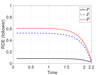
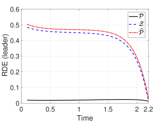
Figure 1: The evolutions of the nonsymmetric coupled RDEs of the follower and the leader for Case I (top: follower, bottom: leader).

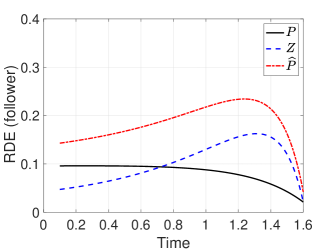
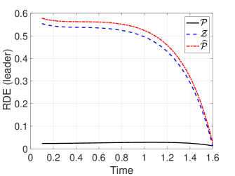
Figure 2: The evolutions of the nonsymmetric coupled RDEs of the follower and the leader for Case II (top: follower, bottom: leader).

As mentioned, it is necessary to check the solvability of the nonsymmetric coupled RDEs of the follower (17) and the leader (32) to characterize the time-consistent Stackelberg equilibrium. This section provides the numerical examples to check their solvability.

We consider the modified resource-allocation Stackelberg game considered in [46, 50], where unlike [50] the time-inconsistent problem is formulated. Specifically, the conditional expectations (mean-field variables) are included in the objective functionals, and the nonexponential discounting is hyperbolic similar to [18]. We consider two different cases:

• $t=0.1$, $T=2.2$, $A=-1.6$, $B_{1}=-0.3$, $B_{2}=1$, $C=0.5$, $D_{1}=D_{2}=0$, $\bar{Q}_{1}=\bar{Q}_{2}=2$, $\bar{R}_{1}=\bar{R}_{2}=0$, $R_{1}(s,t)=(1+0.7(s-t))^{-1.8}$, $R_{2}(s,t)=(1+0.2(s-t))^{-0.3}$, $Q_{1}(s,t)=(5+1.2(s-t))^{-1.2}$, $Q_{2}(s,t)=(10+0.8(s-t))^{-0.5}$, $M_{1}(t)=\bar{M}_{1}(t)=1.3t^{2}$, $M_{2}(t)=\bar{M}_{2}(t)=2.1t^{2}$;

• $t=0.1$, $T=1.6$, $A=-1.6$, $B_{1}=-0.3$, $B_{2}=1$, $C=0.5$, $D_{1}=0.7$, $D_{2}=0.2$, $Q_{1}(s,t)=(5+1.2(s-t))^{-1.2}$, $R_{1}(s,t)=(1+0.7(s-t))^{-1.8}$, $\bar{Q}_{1}=2$, $\bar{R}_{1}(s,t)=(20+3.7(s-t))^{-0.1}$, $Q_{2}(s,t)=(10+0.8(s-t))^{-0.5}$, $R_{2}(s,t)=(1+0.2(s-t))^{-0.3}$, $\bar{Q}_{2}=(0.7+3.1(s-t))^{-1.3}$, $\bar{R}_{2}=25$, $M_{1}(t)=\bar{M}_{1}(t)=1.3t^{2}$, $M_{2}(t)=\bar{M}_{2}(t)=2.1t^{2}$.

Note the hyperbolic cost parameters, $R_{i}$, $\bar{R}_{i}$, $Q_{i}$, $\bar{Q}_{i}$, $M_{i}$ and $\bar{M}_{i}$, in Case I and Case II. It can be seen that Case II is more general in that we consider the controlled diffusion term due to nonzero $D_{1}$ and $D_{2}$, and that the inclusion of the conditional expectation of the controls in the objective functionals. Note that with Case I and Case II, (4) holds. Using the Euler’s method (see [55]), we obtain the plots of the evolutions of the nonsymmetric coupled RDEs of (17) and (32) for Cases I and II, which are depicted in Figs. 1 and 2. These simulation results show that the solutions of the coupled RDEs are well defined and do not have a finite escape time [5]. This implies that in view of Theorems 1 and 3, and Corollary 1, the time-consistent Stackelberg equilibrium for the time-inconsistent resource-allocation problem with Case I and Case II exists, which can be characterized by substituting the parameters in the corresponding case into $u^{*}$ in (29) (equivalently (IV)) and $v^{*}$ in (15) with $u$ replaced by $u^{*}$ in (29).

VI Conclusions

In this paper, we have considered the linear-quadratic (LQ) time-inconsistent mean-field Stackelberg differential game (Problem LQ-TI-MF-SDG). The (time-consistent) equilibrium control of the follower and its state feedback representation in terms of the nonsymmetric coupled RDEs and the BSDE have been obtained. The equilibrium state process of the follower is the FBSDE that captures his rational behavior. Then the leader’s (time-consistent) equilibrium control has been obtained via the variational method under the constraint of the follower’s rational behavior (the FBSDE). The state feedback representation of the leader’s equilibrium control in terms of the nonsymmetric coupled RDEs has been characterized via the generalized decoupling method. Under the solvability of the nonsymmetric coupled RDEs of the leader and the follower, the equilibrium controls of the leader and the follower constitute the time-consistent Stackelberg equilibrium of Problem LQ-TI-MF-SDG. A future research topic is to consider the discrete-time time-inconsistent leader-follower Stackelberg game that can be viewed as an extension of [30]. Another topic would be the existence and uniqueness of the solution to (17) and (32) and their numerical computation approaches. Note that under some assumptions on the coefficients in (17) and (32), the Picard fixed point argument can be used to obtain both existence and uniqueness.

Appendix A Notations for Sections III and IV

The following notation is used in Section III:

$$S(s,s) =[\widehat{R}_{2}(s,s)+D_{2}^{\top}(s)P(s,s)D_{2}(t)\bigr{]}$$

$$H(s) =A(s)-B_{2}(s)S^{-1}(s,s)$$

$$\leavevmode\nobreak\ \leavevmode\nobreak\ \leavevmode\nobreak\ \times\bigl{[}B_{2}^{\top}(s)\widehat{P}(s,s)+D_{2}^{\top}(t)P(s,s)C(s)\bigr{]}$$

$$\bar{H}(s) =C(s)-D_{2}(s)S^{-1}(s,s)$$

$$\leavevmode\nobreak\ \leavevmode\nobreak\ \leavevmode\nobreak\ \times\bigl{[}B_{2}^{\top}(s)\widehat{P}(s,s)+D_{2}^{\top}(t)P(s,s)C(s)\bigr{]}$$

$$\tilde{H}(s,t) =A(s)-B_{2}(s)(S^{-1}(s,s))^{\top}$$

$$\leavevmode\nobreak\ \leavevmode\nobreak\ \leavevmode\nobreak\ \times\bigl{[}B_{2}^{\top}(s)P^{\top}(s,t)+D_{2}^{\top}(s)P^{\top}(s,t)C(s)\bigr{]}$$

$$F(s) =B_{1}(s)-B_{2}(s)S^{-1}(s,s)D_{2}^{\top}(s)P(s,s)D_{1}(s)$$

$$\bar{F}(s) =D_{1}(s)-D_{2}(s)S^{-1}(s,s)D_{2}^{\top}(s)P(s,s)D_{1}(s)$$

$$\tilde{F}(s,t) =C(s)-D_{2}(s)(S^{-1}(s,s))^{\top}$$

$$\leavevmode\nobreak\ \leavevmode\nobreak\ \leavevmode\nobreak\ \times\bigl{[}B_{2}^{\top}(s)P^{\top}(s,t)+D_{2}^{\top}(s)P^{\top}(s,t)C(s)\bigr{]}$$

$$G_{1}(s) =B_{2}(s)S^{-1}(s,s)B_{2}^{\top}(s)$$

$$G_{2}(s) =B_{2}(s)S^{-1}(s,s)D_{2}^{\top}(s)=\bar{G}_{1}^{\top}(s)$$

$$\bar{G}_{2}(s) =D_{2}(s)S^{-1}(s,s)D_{2}^{\top}(s)$$

$$K_{1}(s,t) =D_{1}^{\top}(s)P^{\top}(s,t)C(s)+B_{1}^{\top}(s)P^{\top}(s,t)$$

$$\leavevmode\nobreak\ \leavevmode\nobreak\ \leavevmode\nobreak\ -D_{1}^{\top}(s)P^{\top}(s,s)D_{2}(s)(S^{-1}(s,s))^{\top}$$

$$\leavevmode\nobreak\ \leavevmode\nobreak\ \leavevmode\nobreak\ \times\bigl{[}B_{2}^{\top}(s)P^{\top}(s,t)+D_{2}^{\top}(s)P^{\top}(s,t)C(s)\bigr{]}$$

$$K_{2}(s,t) =B_{1}^{\top}(s)Z^{\top}(s,t)-D_{1}^{\top}(s)P^{\top}(s,s)D_{2}(s)$$ (A.1)

$$\leavevmode\nobreak\ \leavevmode\nobreak\ \leavevmode\nobreak\ \times(S^{-1}(s,s))^{\top}B_{2}^{\top}(s)Z^{\top}(s,t)$$

$$\bar{K}_{1}(s,t) =B_{2}(s)(S^{-1}(s,s))^{\top}(s,s)B_{2}^{\top}(s)Z^{\top}(s,t)$$

$$\bar{K}_{2}(s,t) =D_{2}(s)(S^{-1}(s,s))^{\top}B_{2}^{\top}(s)Z^{\top}(s,t)$$

$$\widehat{R}_{2}(s,t) =R_{2}(s,t)+\bar{R}_{2}(s,t)$$

$$\widehat{M}_{2}(t) =M_{2}(t)+\bar{M}_{2}(t)$$

$$\widehat{Q}_{2}(s,t) =Q_{2}(s,t)+\bar{Q}_{2}(s,t)$$

$$\widehat{P}(s,t) =P(s,t)+Z(s,t).$$

The following notation is used in Section IV:

$$\mathcal{A}_{1}(s,t) =\begin{bmatrix}H(s)&0\\ 0&\tilde{H}(s,t)\end{bmatrix}$$ (A.2)

$$\bar{\mathcal{A}}_{1}(s,t) =\begin{bmatrix}\bar{H}(s)&0\\ 0&\tilde{F}(s,t)\end{bmatrix}$$

$$\mathcal{A}_{2}(s,t) =\begin{bmatrix}0&0\\ 0&-\bar{K}_{1}(s,t)\end{bmatrix}$$

$$\bar{\mathcal{A}}_{2}(s,t) =\begin{bmatrix}0&0\\ 0&-\bar{K}_{2}(s,t)\end{bmatrix}$$

$$\mathcal{B}(s) =\begin{bmatrix}F(s)\\ 0\end{bmatrix},\leavevmode\nobreak\ \bar{\mathcal{B}}(s)=\begin{bmatrix}\bar{F}(s)\\ 0\end{bmatrix}$$

$$\mathcal{C}(s) =\begin{bmatrix}0&-G_{1}(s)\\ G_{1}^{\top}(s)&0\end{bmatrix}$$

$$\bar{\mathcal{C}}(s) =\begin{bmatrix}0&-\bar{G}_{1}(s)\\ G_{2}^{\top}(s)&0\end{bmatrix}$$

$$\mathcal{D}(s) =\begin{bmatrix}0&-G_{2}(s)\\ \bar{G}_{1}^{\top}(s)&0\end{bmatrix}$$

$$\bar{\mathcal{D}}(s) =\begin{bmatrix}0&-\bar{G}_{2}(s)\\ \bar{G}_{2}^{\top}(s)&0\end{bmatrix}$$

$$\mathcal{Q}(s,t) =\begin{bmatrix}Q_{1}(s,t)&0\\ 0&0\end{bmatrix},\leavevmode\nobreak\ \bar{\mathcal{Q}}(s,t)=\begin{bmatrix}\bar{Q}_{1}(s,t)&0\\ 0&0\end{bmatrix}$$

$$\mathcal{G}(s,t) =\begin{bmatrix}0&K_{1}(s,t)\end{bmatrix},\leavevmode\nobreak\ \bar{\mathcal{G}}(s,t)=\begin{bmatrix}0&K_{2}(s,t)\end{bmatrix}$$

$$\mathcal{M}(s) =\begin{bmatrix}M_{1}(s)&0\\ 0&0\end{bmatrix},\leavevmode\nobreak\ \bar{\mathcal{M}}(s)=\begin{bmatrix}\bar{M}_{1}(s)&0\\ 0&0\end{bmatrix}$$

$$X_{0} =\begin{bmatrix}x_{0}\\ 0\end{bmatrix}$$

$$\widehat{\mathcal{R}}(s,t) =\widehat{R}_{1}(s,t)=R_{1}(s,t)+\bar{R}_{1}(s,t)$$

$$\widehat{\mathcal{A}}_{1}(s,t) =\mathcal{A}_{1}(s,t)+\mathcal{A}_{2}(s,t)$$

$$\widehat{\mathcal{A}}_{2}(s,t) =\bar{\mathcal{A}}_{1}(s,t)+\bar{\mathcal{A}}_{2}(s,t).$$

Appendix B Proof of Theorem 2

This appendix provides the proof of Theorem 2.

Proof of Theorem 2: Let $u^{*}$ be given in (22), and the triplet $(x^{*},h^{*},l^{*})$ be the FBSDE in (19) generated by $u^{*}$ (that can be obtained by substituting (22) into (19)). For any $s\in[t,T)$, let $u^{\epsilon}$ be the control defined in (6), and the triplet $(x^{\epsilon},h^{\epsilon},l^{\epsilon})$ be the FBSDE in (19) generated by $u^{\epsilon}$, i.e.,

$$\begin{cases}\differential x^{\epsilon}(s)=\Bigl{[}H(s)x^{\epsilon}(s)+F(s)u^{\epsilon}(s)-G_{1}(s)h^{\epsilon}(s)\\ \leavevmode\nobreak\ \leavevmode\nobreak\ \leavevmode\nobreak\ -G_{2}(s)l^{\epsilon}(s)\Bigr{]}\differential s+\Bigl{[}\bar{H}(s)x^{\epsilon}(s)+\bar{F}(s)u^{\epsilon}(s)\\ \leavevmode\nobreak\ \leavevmode\nobreak\ \leavevmode\nobreak\ -\bar{G}_{1}(s)h^{\epsilon}(s)-\bar{G}_{2}(s)l^{\epsilon}(s)\Bigr{]}\differential B(s),\leavevmode\nobreak\ s\in[t,T]\\ \differential h^{\epsilon}(s)=\Bigl{[}-\tilde{H}^{\top}(s,t)h^{\epsilon}(s)-\tilde{F}^{\top}(s,t)l^{\epsilon}(s)\\ \leavevmode\nobreak\ \leavevmode\nobreak\ \leavevmode\nobreak\ -K_{1}^{\top}(s,t)u^{\epsilon}(s)-K_{2}^{\top}(s,t)\mathbb{E}_{t}[u^{\epsilon}(s)]\\ \leavevmode\nobreak\ \leavevmode\nobreak\ \leavevmode\nobreak\ +\bar{K}_{1}^{\top}(s,t)\mathbb{E}_{t}[h^{\epsilon}(s)]+\bar{K}_{2}^{\top}(s,t)\mathbb{E}_{t}[l^{\epsilon}(s)]\Bigr{]}\differential s\\ \leavevmode\nobreak\ \leavevmode\nobreak\ \leavevmode\nobreak\ +l^{\epsilon}(s)\differential B(s),\leavevmode\nobreak\ s\in[t,T]\\ x^{\epsilon}(t)=x_{0},\leavevmode\nobreak\ h(T)=0.\end{cases}$$

Let $\delta x=x^{*}-x^{\epsilon}$ $\delta h=h^{*}-h^{\epsilon}$, and $\delta l=l^{*}-l^{\epsilon}$. Note that $\delta x(t)=0$ and $\delta h(T)=0$.

By using Itô’s formula, we have

$$\differential\langle\delta x(s),y(s,t)\rangle$$

$$=\langle F(s)(u^{\epsilon}(s)-u^{*}(s))$$

$$\leavevmode\nobreak\ \leavevmode\nobreak\ \leavevmode\nobreak\ -G_{1}(s)\delta h(s)-G_{2}(s)\delta l(s),y(s,t)\rangle\differential s$$

$$\leavevmode\nobreak\ \leavevmode\nobreak\ \leavevmode\nobreak\ +\langle\bar{F}(s)(u^{\epsilon}(s)-u^{*}(s))$$

$$\leavevmode\nobreak\ \leavevmode\nobreak\ \leavevmode\nobreak\ -\bar{G}_{1}(s)\delta h(s)-\bar{G}_{2}(s)\delta l(s),z(s,t)\rangle\differential s$$

$$\leavevmode\nobreak\ \leavevmode\nobreak\ \leavevmode\nobreak\ +\langle\delta x(s),-Q_{1}(s,t)x^{*}(s)-\bar{Q}_{1}(s,t)\mathbb{E}_{t}[x^{*}(s)]\rangle\differential s$$

$$\leavevmode\nobreak\ \leavevmode\nobreak\ \leavevmode\nobreak\ +\langle\bar{H}(s)\delta x(s)+\bar{F}(s)(u^{\epsilon}(s)-u^{*}(s))-\bar{G}_{1}(s)\delta h(s)$$

$$\leavevmode\nobreak\ \leavevmode\nobreak\ \leavevmode\nobreak\ -\bar{G}_{2}(s)\delta l(s),y(s,t)\rangle\differential B(s)+\langle\delta x(s),z(s,t)\rangle\differential B(s),$$

and

$$\differential\langle\delta h(s),\phi(s,t)\rangle$$

$$=\langle-\tilde{H}^{\top}(s,t)\delta h(s)-\tilde{F}^{\top}(s,t)\delta l(s)$$

$$\leavevmode\nobreak\ \leavevmode\nobreak\ \leavevmode\nobreak\ -K_{1}^{\top}(s,t)(u^{\epsilon}(s)-u^{*}(s))$$

$$\leavevmode\nobreak\ \leavevmode\nobreak\ \leavevmode\nobreak\ -K_{2}^{\top}(s,t)\mathbb{E}_{t}[u^{\epsilon}(s)-u^{*}(s)]$$

$$\leavevmode\nobreak\ \leavevmode\nobreak\ \leavevmode\nobreak\ +\bar{K}_{1}^{\top}(s,t)\mathbb{E}_{t}[\delta h(s)]+\bar{K}_{2}^{\top}(s,t)\mathbb{E}_{t}[\delta l(s)],\phi(s,t)\rangle\differential s$$

$$\leavevmode\nobreak\ \leavevmode\nobreak\ \leavevmode\nobreak\ +\langle\delta h(s),\tilde{H}(s,t)\phi(s,t)-\bar{K}_{1}(s,t)\mathbb{E}_{t}[\phi(s,t)]$$

$$\leavevmode\nobreak\ \leavevmode\nobreak\ \leavevmode\nobreak\ +G_{1}^{\top}(s)y(s,t)+\bar{G}_{1}^{\top}(s)z(s,t)\rangle\differential s$$

$$\leavevmode\nobreak\ \leavevmode\nobreak\ \leavevmode\nobreak\ +\langle\delta l(s),\tilde{F}(s,t)\phi(s,t)-\bar{K}_{2}(s,t)\mathbb{E}_{t}[\phi(s,t)]$$

$$\leavevmode\nobreak\ \leavevmode\nobreak\ \leavevmode\nobreak\ +G_{2}^{\top}(s)y(s,t)+\bar{G}_{2}^{\top}(s)z(s,t)\rangle\differential s$$

$$\leavevmode\nobreak\ \leavevmode\nobreak\ \leavevmode\nobreak\ +\langle\delta h(s),\tilde{F}(s,t)\phi(s,t)-\bar{K}_{2}(s,t)\mathbb{E}_{t}[\phi(s,t)]$$

$$\leavevmode\nobreak\ \leavevmode\nobreak\ \leavevmode\nobreak\ +G_{2}^{\top}(s)y(s,t)+\bar{G}_{2}^{\top}(s)z(s,t)\rangle\differential B(s)$$

$$\leavevmode\nobreak\ \leavevmode\nobreak\ \leavevmode\nobreak\ +\langle\delta l(s),\phi(s,t)\rangle\differential B(s).$$

In view of initial and terminal conditions of (20), we have

$$\mathbb{E}_{t}\bigl{[}\langle\delta x(T),M_{1}(t)x^{*}(T)+\bar{M}_{1}(t)\mathbb{E}_{t}[x^{*}(T)]\rangle\bigr{]}$$

$$=\mathbb{E}_{t}\int_{t}^{T}\Bigl{[}\langle F(s)(u^{\epsilon}(s)-u^{*}(s))-G_{1}(s)\delta h(s)$$

$$\leavevmode\nobreak\ \leavevmode\nobreak\ \leavevmode\nobreak\ -G_{2}(s)\delta l(s),y(s,t)\rangle+\langle\bar{F}(s)(u^{\epsilon}(s)-u^{*}(s))$$

$$\leavevmode\nobreak\ \leavevmode\nobreak\ \leavevmode\nobreak\ -\bar{G}_{1}(s)\delta h(s)-\bar{G}_{2}(s)\delta l(s),z(s,t)\rangle$$

$$\leavevmode\nobreak\ \leavevmode\nobreak\ \leavevmode\nobreak\ +\langle\delta x(s),-Q_{1}(s,t)x^{*}(s)-\bar{Q}_{1}(s,t)\mathbb{E}_{t}[x^{*}(s)]\rangle\Bigr{]}\differential s,$$

and

$$0 =\mathbb{E}_{t}\int_{t}^{T}\Bigl{[}\langle-\tilde{H}^{\top}(s,t)\delta h(s)-\tilde{F}^{\top}(s,t)\delta l(s)$$

$$\leavevmode\nobreak\ \leavevmode\nobreak\ \leavevmode\nobreak\ -K_{1}^{\top}(s,t)(u^{\epsilon}(s)-u^{*}(s))$$

$$\leavevmode\nobreak\ \leavevmode\nobreak\ \leavevmode\nobreak\ -K_{2}^{\top}(s,t)\mathbb{E}_{t}[u^{\epsilon}(s)-u^{*}(s)]$$

$$\leavevmode\nobreak\ \leavevmode\nobreak\ \leavevmode\nobreak\ +\bar{K}_{1}^{\top}(s,t)\mathbb{E}_{t}[\delta h(s)]$$

$$\leavevmode\nobreak\ \leavevmode\nobreak\ \leavevmode\nobreak\ +\bar{K}_{2}^{\top}(s,t)\mathbb{E}_{t}[\delta l(s)],\phi(s,t)\rangle$$

$$\leavevmode\nobreak\ \leavevmode\nobreak\ \leavevmode\nobreak\ +\langle\delta h(s),\tilde{H}(s,t)\phi(s,t)-\bar{K}_{1}(s,t)\mathbb{E}_{t}[\phi(s,t)]$$

$$\leavevmode\nobreak\ \leavevmode\nobreak\ \leavevmode\nobreak\ +G_{1}^{\top}(s)y(s,t)+\bar{G}_{1}^{\top}(s)z(s,t)\rangle$$

$$\leavevmode\nobreak\ \leavevmode\nobreak\ \leavevmode\nobreak\ +\langle\delta l(s),\tilde{F}(s,t)\phi(s,t)-\bar{K}_{2}(s,t)\mathbb{E}_{t}[\phi(s,t)]$$

$$\leavevmode\nobreak\ \leavevmode\nobreak\ \leavevmode\nobreak\ +G_{2}^{\top}(s)y(s,t)+\bar{G}_{2}^{\top}(s)z(s,t)\rangle\Bigr{]}\differential s$$

$$=\mathbb{E}_{t}\int_{t}^{T}\Bigl{[}\langle-K_{1}^{\top}(s,t)(u^{\epsilon}(s)-u^{*}(s))$$

$$\leavevmode\nobreak\ \leavevmode\nobreak\ \leavevmode\nobreak\ -K_{2}^{\top}(s,t)\mathbb{E}_{t}[u^{\epsilon}(s)-u^{*}(s)],\phi(s,t)\rangle$$

$$\leavevmode\nobreak\ \leavevmode\nobreak\ \leavevmode\nobreak\ +\langle\delta h(s),G_{1}^{\top}(s)y(s,t)+\bar{G}_{1}^{\top}(s)z(s,t)\rangle$$

$$\leavevmode\nobreak\ \leavevmode\nobreak\ \leavevmode\nobreak\ +\langle\delta l(s),G_{2}^{\top}(s)y(s,t)+\bar{G}_{2}^{\top}(s)z(s,t)\rangle\Bigr{]}\differential s,$$

which implies

$$\mathbb{E}_{t}\bigl{[}\langle\delta x(T),M_{1}(t)x^{*}(T)+\bar{M}_{1}(t)\mathbb{E}_{t}[x^{*}(T)]\rangle\bigr{]}$$ (B.1)

$$=\mathbb{E}_{t}\int_{t}^{T}\Bigl{[}\langle F(s)(u^{\epsilon}(s)-u^{*}(s)),y(s,t)\rangle$$

$$\leavevmode\nobreak\ \leavevmode\nobreak\ \leavevmode\nobreak\ +\langle\bar{F}(s)(u^{\epsilon}(s)-u^{*}(s)),z(s,t)\rangle$$

$$\leavevmode\nobreak\ \leavevmode\nobreak\ \leavevmode\nobreak\ +\langle-K_{1}^{\top}(s,t)(u^{\epsilon}(s)-u^{*}(s))$$

$$\leavevmode\nobreak\ \leavevmode\nobreak\ \leavevmode\nobreak\ -K_{2}^{\top}(s,t)\mathbb{E}_{t}[u^{\epsilon}(s)-u^{*}(s)],\phi(s,t)\rangle$$

$$\leavevmode\nobreak\ \leavevmode\nobreak\ \leavevmode\nobreak\ +\langle\delta x(s),-Q_{1}(s,t)x^{*}(s)-\bar{Q}_{1}(s,t)\mathbb{E}_{t}[x^{*}(s)]\rangle\Bigr{]}\differential s.$$

On the other hand, for the objective functional of the leader in (2), we have

$$J_{1}(t,x_{0};u^{\epsilon},\alpha[u^{\epsilon},x_{0}])-J_{1}(t,x_{0};u^{*},\alpha[u^{*},x_{0}])$$

$$=\mathbb{E}_{t}\Biggl{[}\int_{t}^{T}\Bigl{[}\langle x^{\epsilon}(s)+x^{*}(s),Q_{1}(s,t)\delta x(s)\rangle$$

$$\leavevmode\nobreak\ \leavevmode\nobreak\ \leavevmode\nobreak\ +\langle\mathbb{E}_{t}[x^{\epsilon}(s)+x^{*}(s)],\bar{Q}_{1}(s,t)\mathbb{E}_{t}[\delta x(s)]\rangle$$

$$\leavevmode\nobreak\ \leavevmode\nobreak\ \leavevmode\nobreak\ +\langle u^{\epsilon}(s)+u^{*}(s),R_{1}(s,t)(u^{\epsilon}(s)-u^{*}(s))\rangle$$

$$\leavevmode\nobreak\ \leavevmode\nobreak\ \leavevmode\nobreak\ +\langle\mathbb{E}_{t}[u^{\epsilon}(s)+u^{*}(s)],\bar{R}_{1}(s,t)\mathbb{E}_{t}[u^{\epsilon}(s)-u^{*}(s)]\rangle\Bigr{]}\differential s$$

$$\leavevmode\nobreak\ \leavevmode\nobreak\ \leavevmode\nobreak\ +\langle x^{\epsilon}(T)+x^{*}(T),M_{1}(t)\delta x(T)\rangle$$

$$\leavevmode\nobreak\ \leavevmode\nobreak\ \leavevmode\nobreak\ +\langle\mathbb{E}_{t}[x^{\epsilon}(T)+x^{*}(T)],\bar{M}_{1}(t)\mathbb{E}_{t}[\delta x(T)]\rangle\Biggr{]}.$$

Hence, with (B.1), we have

$$J_{1}(t,x_{0};u^{\epsilon},\alpha[u^{\epsilon},x_{0}])-J_{1}(t,x_{0};u^{*},\alpha[u^{*},x_{0}])$$ (B.2)

$$=\mathbb{E}_{t}\Biggl{[}\int_{t}^{T}\Bigl{[}\langle x^{\epsilon}(s)+x^{*}(s),Q_{1}(s,t)\delta x(s)\rangle$$

$$\leavevmode\nobreak\ \leavevmode\nobreak\ \leavevmode\nobreak\ +\langle\mathbb{E}_{t}[x^{\epsilon}(s)+x^{*}(s)],\bar{Q}_{1}(s,t)\mathbb{E}_{t}[\delta x(s)]\rangle$$

$$\leavevmode\nobreak\ \leavevmode\nobreak\ \leavevmode\nobreak\ +\langle u^{\epsilon}(s)+u^{*}(s),R_{1}(s,t)(u^{\epsilon}(s)-u^{*}(s))\rangle$$

$$\leavevmode\nobreak\ \leavevmode\nobreak\ \leavevmode\nobreak\ +\langle\mathbb{E}_{t}[u^{\epsilon}(s)+u^{*}(s)],\bar{R}_{1}(s,t)\mathbb{E}_{t}[u^{\epsilon}(s)-u^{*}(s)]\rangle\Bigr{]}\differential s$$

$$\leavevmode\nobreak\ \leavevmode\nobreak\ \leavevmode\nobreak\ +\langle x^{\epsilon}(T)+x^{*}(T),M_{1}(t)\delta x(T)\rangle$$

$$\leavevmode\nobreak\ \leavevmode\nobreak\ \leavevmode\nobreak\ +\langle\mathbb{E}_{t}[x^{\epsilon}(T)+x^{*}(T)],\bar{M}_{1}(t)\mathbb{E}_{t}[\delta x(T)]\rangle\Biggr{]}$$

$$\leavevmode\nobreak\ \leavevmode\nobreak\ \leavevmode\nobreak\ +2\mathbb{E}_{t}\int_{t}^{T}\Bigl{[}\langle F(s)(u^{\epsilon}(s)-u^{*}(s)),y(s,t)\rangle$$

$$\leavevmode\nobreak\ \leavevmode\nobreak\ \leavevmode\nobreak\ +\langle\bar{F}(s)(u^{\epsilon}(s)-u^{*}(s)),z(s,t)\rangle$$

$$\leavevmode\nobreak\ \leavevmode\nobreak\ \leavevmode\nobreak\ +\langle-K_{1}^{\top}(s,t)(u^{\epsilon}(s)-u^{*}(s))$$

$$\leavevmode\nobreak\ \leavevmode\nobreak\ \leavevmode\nobreak\ -K_{2}^{\top}(s,t)\mathbb{E}_{t}[u^{\epsilon}(s)-u^{*}(s)],\phi(s,t)\rangle$$

$$\leavevmode\nobreak\ \leavevmode\nobreak\ \leavevmode\nobreak\ +\langle\delta x(s),-Q_{1}(s,t)x^{*}(s)-\bar{Q}_{1}(s,t)\mathbb{E}_{t}[x^{*}(s)]\rangle\Bigr{]}\differential s$$

$$\leavevmode\nobreak\ \leavevmode\nobreak\ \leavevmode\nobreak\ -2\mathbb{E}_{t}\bigl{[}\langle\delta x(T),M_{1}(t)x^{*}(T)+\bar{M}_{1}(t)\mathbb{E}_{t}[x^{*}(T)]\rangle\bigr{]}$$

$$=\mathbb{E}_{t}\Biggl{[}\int_{t}^{T}\Bigl{[}\langle Q_{1}(s,t)(x^{\epsilon}(s)+x^{*}(s)),\delta x(s)\rangle$$

$$\leavevmode\nobreak\ \leavevmode\nobreak\ \leavevmode\nobreak\ +\langle-2Q_{1}(s,t)x^{*}(s),\delta x(s)\rangle$$

$$\leavevmode\nobreak\ \leavevmode\nobreak\ \leavevmode\nobreak\ +\langle\bar{Q}_{1}(s,t)\mathbb{E}_{t}[x^{\epsilon}(s)+x^{*}(s)],\delta x(s)\rangle$$

$$\leavevmode\nobreak\ \leavevmode\nobreak\ \leavevmode\nobreak\ +\langle-2\bar{Q}_{1}(s,t)\mathbb{E}_{t}[x^{*}(s)],\delta x(s)\rangle$$

$$\leavevmode\nobreak\ \leavevmode\nobreak\ \leavevmode\nobreak\ +\langle R_{1}(s,t)(u^{\epsilon}(s)+u^{*}(s)),u^{\epsilon}(s)-u^{*}(s)\rangle$$

$$\leavevmode\nobreak\ \leavevmode\nobreak\ \leavevmode\nobreak\ +\langle\bar{R}_{1}(s,t)\mathbb{E}_{t}[u^{\epsilon}(s)+u^{*}(s)],u^{\epsilon}(s)-u^{*}(s)\rangle$$

$$\leavevmode\nobreak\ \leavevmode\nobreak\ \leavevmode\nobreak\ +2\langle F^{\top}(s)y(s,t)+\bar{F}^{\top}(s)z(s,t),u^{\epsilon}(s)-u^{*}(s)\rangle$$

$$\leavevmode\nobreak\ \leavevmode\nobreak\ \leavevmode\nobreak\ +2\langle-K_{1}(s,t)\phi(s,t)-K_{2}(s,t)\mathbb{E}_{t}[\phi(s,t)],$$

$$\leavevmode\nobreak\ \leavevmode\nobreak\ \leavevmode\nobreak\ u^{\epsilon}(s)-u^{*}(s)\rangle\Bigr{]}\differential s$$

$$\leavevmode\nobreak\ \leavevmode\nobreak\ \leavevmode\nobreak\ +\langle M_{1}(t)(x^{\epsilon}(T)+x^{*}(T)),\delta x(T)\rangle$$

$$\leavevmode\nobreak\ \leavevmode\nobreak\ \leavevmode\nobreak\ +\langle\bar{M}_{1}(t)\mathbb{E}_{t}[x^{\epsilon}(T)+x^{*}(T)],\delta x(T)\rangle$$

$$\leavevmode\nobreak\ \leavevmode\nobreak\ \leavevmode\nobreak\ -2\langle M_{1}(t)x^{*}(T)+\bar{M}_{1}(t)\mathbb{E}_{t}[x^{*}(T)],\delta x(s)\rangle\Biggr{]}.$$

Then with $\widehat{Q}_{1}(s,t)=Q_{1}(s,t)+\bar{Q}_{1}(s,t)$ and $\widehat{M}_{1}(s,t)=M_{1}(s,t)+\bar{M}_{1}(s,t)$ and due to the definition of the perturbed control in (6), (B.2) can be rewritten as

$$J_{1}(t,x_{0};u^{\epsilon},\alpha[u^{\epsilon},x_{0}])-J_{1}(t,x_{0};u^{*},\alpha[u^{*},x_{0}])$$ (B.3)

$$=\mathbb{E}_{t}\Biggl{[}\int_{t}^{T}\Bigl{[}|\delta x(s)-\mathbb{E}_{t}[\delta x(s)]|^{2}_{Q_{1}(s,t)}$$

$$\leavevmode\nobreak\ \leavevmode\nobreak\ \leavevmode\nobreak\ +|\mathbb{E}_{t}[\delta x(s)]|^{2}_{\widehat{Q}_{1}(s,t)}\Bigr{]}\differential s+|\mathbb{E}_{t}[\delta x(T)]|^{2}_{\widehat{M}_{1}(t)}$$

$$\leavevmode\nobreak\ \leavevmode\nobreak\ \leavevmode\nobreak\ +|\delta x(T)-\mathbb{E}_{t}[\delta x(T)]|^{2}_{M_{1}(t)}$$

$$\leavevmode\nobreak\ \leavevmode\nobreak\ \leavevmode\nobreak\ +\int_{t}^{t+\epsilon}\Bigl{[}\langle R_{1}(s,t)(u^{\epsilon}(s)+u^{*}(s)),u^{\epsilon}(s)-u^{*}(s)\rangle$$

$$\leavevmode\nobreak\ \leavevmode\nobreak\ \leavevmode\nobreak\ +\langle\bar{R}_{1}(s,t)\mathbb{E}_{t}[u^{\epsilon}(s)+u^{*}(s)],u^{\epsilon}(s)-u^{*}(s)\rangle$$

$$\leavevmode\nobreak\ \leavevmode\nobreak\ \leavevmode\nobreak\ +2\langle F^{\top}(s)y(s,t)+\bar{F}^{\top}(s)z(s,t),u^{\epsilon}(s)-u^{*}(s)\rangle$$

$$\leavevmode\nobreak\ \leavevmode\nobreak\ \leavevmode\nobreak\ +2\langle-K_{1}(s,t)\phi(s,t)-K_{2}(s,t)\mathbb{E}_{t}[\phi(s,t)],$$

$$\leavevmode\nobreak\ \leavevmode\nobreak\ \leavevmode\nobreak\ u^{\epsilon}(s)-u^{*}(s)\rangle\Bigr{]}\differential s\Biggr{]}.$$

Note that

$$\mathbb{E}_{t}\Bigl{[}\langle R_{1}(s,t)(u^{\epsilon}(s)+u^{*}(s)),u^{\epsilon}(s)-u^{*}(s)\rangle$$ (B.4)

$$\leavevmode\nobreak\ \leavevmode\nobreak\ \leavevmode\nobreak\ +\langle\bar{R}_{1}(s,t)\mathbb{E}_{t}[u^{\epsilon}(s)+u^{*}(s)],u^{\epsilon}(s)-u^{*}(s)\rangle$$

$$\leavevmode\nobreak\ \leavevmode\nobreak\ \leavevmode\nobreak\ +2\langle F^{\top}(s)y(s,t)+\bar{F}^{\top}(s)z(s,t),u^{\epsilon}(s)-u^{*}(s)\rangle$$

$$\leavevmode\nobreak\ \leavevmode\nobreak\ \leavevmode\nobreak\ +2\langle-K_{1}(s,t)\phi(s,t)-K_{2}(s,t)\mathbb{E}_{t}[\phi(s,t)],$$

$$\leavevmode\nobreak\ \leavevmode\nobreak\ \leavevmode\nobreak\ u^{\epsilon}(s)-u^{*}(s)\rangle\Bigr{]}$$

$$=\mathbb{E}_{t}\Bigl{[}\langle R_{1}(s,t)(u^{\epsilon}(s)-u^{*}(s)),u^{\epsilon}(s)-u^{*}(s)\rangle$$

$$\leavevmode\nobreak\ \leavevmode\nobreak\ \leavevmode\nobreak\ +\langle\bar{R}_{1}(s,t)\mathbb{E}_{t}[u^{\epsilon}(s)-u^{*}(s)],u^{\epsilon}(s)-u^{*}(s)\rangle$$

$$\leavevmode\nobreak\ \leavevmode\nobreak\ \leavevmode\nobreak\ +2\langle R_{1}(s,t)u^{*}(s)+\bar{R}_{1}(s,t)\mathbb{E}_{t}[u^{*}(s)],$$

$$\leavevmode\nobreak\ \leavevmode\nobreak\ \leavevmode\nobreak\ u^{\epsilon}(s)-u^{*}(s)\rangle$$

$$\leavevmode\nobreak\ \leavevmode\nobreak\ \leavevmode\nobreak\ +2\langle F^{\top}(s)y(s,t)+\bar{F}^{\top}(s)z(s,t),u^{\epsilon}(s)-u^{*}(s)\rangle$$

$$\leavevmode\nobreak\ \leavevmode\nobreak\ \leavevmode\nobreak\ +2\langle-K_{1}(s,t)\phi(s,t)-K_{2}(s,t)\mathbb{E}_{t}[\phi(s,t)],$$

$$\leavevmode\nobreak\ \leavevmode\nobreak\ \leavevmode\nobreak\ u^{\epsilon}(s)-u^{*}(s)\rangle\Bigr{]}$$

$$=\mathbb{E}_{t}\Bigl{[}|(u^{\epsilon}(s)-u^{*}(s))-\mathbb{E}_{t}[u^{\epsilon}(s)-u^{*}(s)]|^{2}_{R_{1}(s,t)}$$

$$\leavevmode\nobreak\ \leavevmode\nobreak\ \leavevmode\nobreak\ +|\mathbb{E}_{t}[u^{\epsilon}(s)-u^{*}(s)]|^{2}_{\widehat{R}_{1}(s,t)}$$

$$\leavevmode\nobreak\ \leavevmode\nobreak\ \leavevmode\nobreak\ +2\langle\lambda(s,t),u^{\epsilon}(s)-u^{*}(s)\rangle\Bigr{]},$$

where

$$\lambda(s,t) =R_{1}(s,t)u^{*}(s)+\bar{R}_{1}(s,t)\mathbb{E}_{t}[u^{*}(s)]$$

$$\leavevmode\nobreak\ \leavevmode\nobreak\ \leavevmode\nobreak\ +F^{\top}(s)y(s,t)+\bar{F}^{\top}(s)z(s,t)$$

$$\leavevmode\nobreak\ \leavevmode\nobreak\ \leavevmode\nobreak\ -K_{1}(s,t)\phi(s,t)-K_{2}(s,t)\mathbb{E}_{t}[\phi(s,t)].$$

Due to the definition of $u^{*}$ in (22), boundedness of the coefficients, and the continuity of the FBSDEs in (19) and (20), we have

$$\liminf_{s\downarrow t}\mathbb{E}[|\lambda(s,t)|^{2}]=0.$$ (B.5)

Hence, (B.4) can be rewritten as follows:

$$\mathbb{E}_{t}\Bigl{[}|(u^{\epsilon}(s)-u^{*}(s))-\mathbb{E}_{t}[u^{\epsilon}(s)-u^{*}(s)]|^{2}_{R_{1}(s,t)}$$

$$\leavevmode\nobreak\ \leavevmode\nobreak\ \leavevmode\nobreak\ +|\mathbb{E}_{t}[u^{\epsilon}(s)-u^{*}(s)]|^{2}_{\widehat{R}_{1}(s,t)}$$

$$\leavevmode\nobreak\ \leavevmode\nobreak\ \leavevmode\nobreak\ +2\langle\lambda(s,t),u^{\epsilon}(s)-u^{*}(s)-\mathbb{E}_{t}[u^{\epsilon}(s)-u^{*}(s)]$$

$$\leavevmode\nobreak\ \leavevmode\nobreak\ \leavevmode\nobreak\ +\mathbb{E}_{t}[u^{\epsilon}(s)-u^{*}(s)]\rangle\Bigr{]}$$

$$=\mathbb{E}_{t}\Biggl{[}\Bigl{|}R_{1}^{\frac{1}{2}}(s,t)(u^{\epsilon}(s)-u^{*}(s))$$

$$\leavevmode\nobreak\ \leavevmode\nobreak\ \leavevmode\nobreak\ -R_{1}^{\frac{1}{2}}(s,t)\mathbb{E}_{t}[u^{\epsilon}(s)-u^{*}(s)]+R_{1}^{-\frac{1}{2}}(s,t)\lambda(s,t)\Bigr{|}^{2}$$

$$\leavevmode\nobreak\ \leavevmode\nobreak\ \leavevmode\nobreak\ +\Bigl{|}\widehat{R}_{1}^{\frac{1}{2}}(s,t)\mathbb{E}_{t}[u^{\epsilon}(s)-u^{*}(s)]+\widehat{R}_{1}^{-\frac{1}{2}}(s,t)\mathbb{E}_{t}[\lambda(s,t)]\Bigr{|}^{2}$$

$$\leavevmode\nobreak\ \leavevmode\nobreak\ \leavevmode\nobreak\ -\bigl{|}\lambda(s,t)\bigr{|}^{2}_{R_{1}^{-1}(s,t)}-\bigl{|}\mathbb{E}_{t}[\lambda(s,t)]\bigr{|}^{2}_{\widehat{R}_{1}^{-1}(s,t)}\Biggr{]}.$$

This and (B.3) lead to

$$J_{1}(t,x_{0};u^{\epsilon},\alpha[u^{\epsilon},x_{0}])-J_{1}(t,x_{0};u^{*},\alpha[u^{*},x_{0}])$$

$$=\mathbb{E}_{t}\Biggl{[}\int_{t}^{T}\Bigl{[}|\delta x(s)-\mathbb{E}_{t}[\delta x(s)]|^{2}_{Q_{1}(s,t)}$$

$$\leavevmode\nobreak\ \leavevmode\nobreak\ \leavevmode\nobreak\ +|\mathbb{E}_{t}[\delta x(s)]|^{2}_{\widehat{Q}_{1}(s,t)}\Bigr{]}\differential s+|\mathbb{E}_{t}[\delta x(T)]|^{2}_{\widehat{M}_{1}(t)}$$

$$\leavevmode\nobreak\ \leavevmode\nobreak\ \leavevmode\nobreak\ +|\delta x(T)-\mathbb{E}_{t}[\delta x(T)]|^{2}_{M_{1}(t)}$$

$$\leavevmode\nobreak\ \leavevmode\nobreak\ \leavevmode\nobreak\ +\int_{t}^{t+\epsilon}\Bigl{[}\Bigl{|}R_{1}^{\frac{1}{2}}(s,t)(u^{\epsilon}(s)-u^{*}(s))$$

$$\leavevmode\nobreak\ \leavevmode\nobreak\ \leavevmode\nobreak\ -R_{1}^{\frac{1}{2}}(s,t)\mathbb{E}_{t}[u^{\epsilon}(s)-u^{*}(s)]+R_{1}^{-\frac{1}{2}}(s,t)\lambda(s,t)\Bigr{|}^{2}$$

$$\leavevmode\nobreak\ \leavevmode\nobreak\ \leavevmode\nobreak\ +\Bigl{|}\widehat{R}_{1}^{\frac{1}{2}}(s,t)\mathbb{E}_{t}[u^{\epsilon}(s)-u^{*}(s)]+\widehat{R}_{1}^{-\frac{1}{2}}(s,t)\mathbb{E}_{t}[\lambda(s,t)]\Bigr{|}^{2}$$

$$\leavevmode\nobreak\ \leavevmode\nobreak\ \leavevmode\nobreak\ -\bigl{|}\lambda(s,t)\bigr{|}^{2}_{R_{1}^{-1}(s,t)}-\bigl{|}\mathbb{E}_{t}[\lambda(s,t)]\bigr{|}^{2}_{\widehat{R}^{-1}_{1}(s,t)}\Bigr{]}\differential s\Biggr{]}$$

$$\geq-\mathbb{E}_{t}\int_{t}^{t+\epsilon}\Bigl{[}\bigl{|}\lambda(s,t)\bigr{|}^{2}_{R_{1}^{-1}(s,t)}+\bigl{|}\mathbb{E}_{t}[\lambda(s,t)]\bigr{|}^{2}_{\widehat{R}_{1}^{-1}(s,t)}\Bigr{]}\differential s,$$

which, together with (B.5), implies

$$\liminf_{\epsilon\downarrow 0}\frac{1}{\epsilon}\Bigl{(}J_{1}(t,x_{0};u^{\epsilon},\alpha[u^{\epsilon},x_{0}])$$

$$\leavevmode\nobreak\ \leavevmode\nobreak\ \leavevmode\nobreak\ -J_{1}(t,x_{0};u^{*},\alpha[u^{*},x_{0}])\Bigr{)}\geq 0$$

Hence, in view of Definition 2(ii), we have the desired result. This completes the proof. $\hfill{\square}$

Appendix C Explicit Expressions of the Nonsymmetric Coupled RDEs in (32)

In this appendix, we provide the explicit expressions of nonsymmetric coupled RDEs in (32).

In (32), we have

$$\begin{cases}-\frac{\differential\mathcal{P}(s,t)}{\differential s}=\Lambda_{1}(s,t,\mathcal{P}(s,t),\mathcal{Z}(s,t)),\leavevmode\nobreak\ s\in[t,T]\\ -\frac{\differential\mathcal{Z}(s,t)}{\differential s}=\Lambda_{2}(s,t,\mathcal{P}(s,t),\mathcal{Z}(s,t)),\leavevmode\nobreak\ s\in[t,T]\\ \mathcal{P}(T,t)=\mathcal{M}(t),\leavevmode\nobreak\ \mathcal{Z}(T,t)=\bar{\mathcal{M}}(t)\\ \det(I-\mathcal{P}(s,t)\bar{\mathcal{D}}(s))\neq 0\\ \det\bigl(\widehat{\mathcal{R}}(t,t)+\bar{\mathcal{B}}^{\top}(t)\bigl{[}I-\mathcal{P}(t,t)\bar{\mathcal{D}}(t)\bigr{]}^{-1}\mathcal{P}(t,t)\bar{\mathcal{B}}(t)\bigr{missing})\neq 0\\ \widehat{\mathcal{P}}(s,t)=\mathcal{P}(s,t)+\mathcal{Z}(s,t),\end{cases}$$

where

$$\Lambda_{1}(s,t,\mathcal{P}(s,t),\mathcal{Z}(s,t))$$ (C.1)

$$=\mathcal{A}_{1}^{\top}(s)\mathcal{P}(s,t)+\mathcal{P}(s,t)\mathcal{A}_{1}(s)+\mathcal{Q}(s,t)$$

$$\leavevmode\nobreak\ \leavevmode\nobreak\ \leavevmode\nobreak\ +\mathcal{P}(s,t)\mathcal{C}(s)\mathcal{P}(s,t)+\Bigl{[}\bar{\mathcal{A}}_{1}^{\top}(s,t)+\mathcal{P}(s,t)\mathcal{D}(s)\Bigr{]}$$

$$\leavevmode\nobreak\ \leavevmode\nobreak\ \leavevmode\nobreak\ \times\Bigl{[}I-\mathcal{P}(s,t)\bar{\mathcal{D}}(s)\Bigr{]}^{-1}\mathcal{P}(s,t)\Bigl{(}\bar{\mathcal{A}}_{1}(s,t)$$

$$\leavevmode\nobreak\ \leavevmode\nobreak\ \leavevmode\nobreak\ -\bar{\mathcal{B}}(s)\Bigl{[}\widehat{\mathcal{R}}(s,s)+\bar{\mathcal{B}}^{\top}(s)\bigl{[}I-\mathcal{P}(s,s)\bar{\mathcal{D}}(s)\bigr{]}^{-1}\mathcal{P}(s,s)\bar{\mathcal{B}}(s)\Bigr{]}^{-1}$$

$$\leavevmode\nobreak\ \leavevmode\nobreak\ \leavevmode\nobreak\ \times\Bigl{[}\mathcal{B}^{\top}(s)\widehat{\mathcal{P}}(s,s)+\bar{\mathcal{B}}^{\top}(s)\bigl{[}I-\mathcal{P}(s,s)\bar{\mathcal{D}}(s)\bigr{]}^{-1}$$

$$\leavevmode\nobreak\ \leavevmode\nobreak\ \leavevmode\nobreak\ \times\mathcal{P}(s,s)(\widehat{\mathcal{A}}_{2}(s,s)+\bar{\mathcal{C}}(s)\widehat{\mathcal{P}}(s,s))\Bigr{]}+\bar{\mathcal{C}}(s)\mathcal{P}(s,t)\Bigr{)}$$

$$\leavevmode\nobreak\ \leavevmode\nobreak\ \leavevmode\nobreak\ -\Bigl{[}\mathcal{G}^{\top}(s,t)+\mathcal{P}(s,t)\mathcal{B}(s)\Bigr{]}$$

$$\leavevmode\nobreak\ \leavevmode\nobreak\ \leavevmode\nobreak\ \times\Bigl{[}\widehat{\mathcal{R}}(s,s)+\bar{\mathcal{B}}^{\top}(s)\bigl{[}I-\mathcal{P}(s,s)\bar{\mathcal{D}}(s)\bigr{]}^{-1}\mathcal{P}(s,s)\bar{\mathcal{B}}(s)\Bigr{]}^{-1}$$

$$\leavevmode\nobreak\ \leavevmode\nobreak\ \leavevmode\nobreak\ \times\Bigl{[}\mathcal{B}^{\top}(s)\widehat{\mathcal{P}}(s,s)+\bar{\mathcal{B}}^{\top}(s)\bigl{[}I-\mathcal{P}(s,s)\bar{\mathcal{D}}(s)\bigr{]}^{-1}$$

$$\leavevmode\nobreak\ \leavevmode\nobreak\ \leavevmode\nobreak\ \times\mathcal{P}(s,s)(\widehat{\mathcal{A}}_{2}(s,s)+\bar{\mathcal{C}}(s)\widehat{\mathcal{P}}(s,s))\Bigr{]},$$

and

$$\Lambda_{2}(s,t,\mathcal{P}(s,t),\mathcal{Z}(s,t))$$ (C.2)

$$=\mathcal{A}_{1}^{\top}(s,t)\mathcal{Z}(s,t)+\mathcal{A}_{2}^{\top}(s,t)\widehat{\mathcal{P}}(s,t)+\mathcal{P}(s,t)\mathcal{A}_{2}(s,t)$$

$$\leavevmode\nobreak\ \leavevmode\nobreak\ \leavevmode\nobreak\ +\mathcal{Z}(s,t)\widehat{\mathcal{A}}_{1}(s,t)+\bar{\mathcal{Q}}(s,t)$$

$$\leavevmode\nobreak\ \leavevmode\nobreak\ \leavevmode\nobreak\ +\mathcal{P}(s,t)\mathcal{C}(s)\mathcal{Z}(s,t)+\mathcal{Z}(s,t)\mathcal{C}(s)\widehat{\mathcal{P}}(s,t)$$

$$\leavevmode\nobreak\ \leavevmode\nobreak\ \leavevmode\nobreak\ +\Bigl{[}\bar{\mathcal{A}}_{1}^{\top}(s,t)+\mathcal{P}(s,t)\mathcal{D}(s)\Bigr{]}\Bigl{[}I-\mathcal{P}(s,t)\bar{\mathcal{D}}(s)\Bigr{]}^{-1}\mathcal{P}(s,t)$$

$$\leavevmode\nobreak\ \leavevmode\nobreak\ \leavevmode\nobreak\ \times\Bigl{[}\bar{\mathcal{A}}_{2}(s,t)+\bar{\mathcal{C}}(s)\mathcal{Z}(s,t)\Bigr{]}$$

$$\leavevmode\nobreak\ \leavevmode\nobreak\ \leavevmode\nobreak\ +\Bigl{[}\bar{\mathcal{A}}_{2}^{\top}(s,t)+\mathcal{Z}(s,t)\mathcal{D}(s)\Bigr{]}\Bigl{[}I-\mathcal{P}(s,t)\bar{\mathcal{D}}(s)\Bigr{]}^{-1}\mathcal{P}(s,t)$$

$$\leavevmode\nobreak\ \leavevmode\nobreak\ \leavevmode\nobreak\ \times\Bigl{(}\widehat{\mathcal{A}}_{2}(s,t)+\bar{\mathcal{C}}(s)\widehat{\mathcal{P}}(s,t)-\bar{\mathcal{B}}(s)$$

$$\leavevmode\nobreak\ \leavevmode\nobreak\ \leavevmode\nobreak\ \times\Bigl{[}\widehat{\mathcal{R}}(s,s)+\bar{\mathcal{B}}^{\top}(s)\bigl{[}I-\mathcal{P}(s,s)\bar{\mathcal{D}}(s)\bigr{]}^{-1}\mathcal{P}(s,s)\bar{\mathcal{B}}(s)\Bigr{]}^{-1}$$

$$\leavevmode\nobreak\ \leavevmode\nobreak\ \leavevmode\nobreak\ \times\Bigl{[}\mathcal{B}^{\top}(s)\widehat{\mathcal{P}}(s,s)+\bar{\mathcal{B}}^{\top}(s)\bigl{[}I-\mathcal{P}(s,s)\bar{\mathcal{D}}(s)\bigr{]}^{-1}$$

$$\leavevmode\nobreak\ \leavevmode\nobreak\ \leavevmode\nobreak\ \times\mathcal{P}(s,s)(\widehat{\mathcal{A}}_{2}(s,s)+\bar{\mathcal{C}}(s)\widehat{\mathcal{P}}(s,s))\Bigr{]}\Bigr{)}$$

$$\leavevmode\nobreak\ \leavevmode\nobreak\ \leavevmode\nobreak\ -\Bigl{[}\bar{\mathcal{G}}^{\top}(s,t)+\mathcal{Z}(s,t)\mathcal{B}(s)\Bigr{]}$$

$$\leavevmode\nobreak\ \leavevmode\nobreak\ \leavevmode\nobreak\ \times\Bigl{[}\widehat{\mathcal{R}}(s,s)+\bar{\mathcal{B}}^{\top}(s)\bigl{[}I-\mathcal{P}(s,s)\bar{\mathcal{D}}(s)\bigr{]}^{-1}\mathcal{P}(s,s)\bar{\mathcal{B}}(s)\Bigr{]}^{-1}$$

$$\leavevmode\nobreak\ \leavevmode\nobreak\ \leavevmode\nobreak\ \times\Bigl{(}\mathcal{B}^{\top}(s)\widehat{\mathcal{P}}(s,s)+\bar{\mathcal{B}}^{\top}(s)\bigl{[}I-\mathcal{P}(s,s)\bar{\mathcal{D}}(s)\bigr{]}^{-1}$$

$$\leavevmode\nobreak\ \leavevmode\nobreak\ \leavevmode\nobreak\ \times\mathcal{P}(s,s)(\widehat{\mathcal{A}}_{2}(s,s)+\bar{\mathcal{C}}(s)\widehat{\mathcal{P}}(s,s))\Bigr{)}.$$

Hence, we have

$$\begin{cases}\widehat{\mathcal{P}}(s,t)=\mathcal{P}(s,t)+\mathcal{Z}(s,t)\\ \frac{\differential\widehat{\mathcal{P}}(s,t)}{\differential s}=\Lambda_{3}(s,t,\mathcal{P}(s,t),\mathcal{Z}(s,t)),\leavevmode\nobreak\ s\in[t,T]\\ \widehat{\mathcal{P}}(T,t)=\mathcal{M}(t)+\bar{\mathcal{M}}(t),\end{cases}$$ (C.3)

where the explicit expression of $\Lambda_{3}$ can be obtained from (C.1) and (C.2).

References

• [1] Y. Hu, H. Jin, and X. Y. Zhou, “Time-inconsistent stochastic linear-quadratic control,” SIAM J. Control and Optimization, vol. 50, no. 3, pp. 1548–1572, 2012.
• [2] J. Yong, “Deterministic time-inconsistent optimal control problems - an essentially cooperative approach,” Acta Mathematicae Applicatae Sinica, vol. 28, no. 1, pp. 1–30, 2012.
• [3] ——, “Linear-quadratic optimal control problems for mean-field stochastic differential equations–time-consistent solutions,” Trans. on the American Mathematical Society, vol. 369, no. 8, pp. 5467–5523, 2017.
• [4] W. Yan and J. Yong, Modeling, Stochastic Control, Optimization, and Applications.   Springer, 2019, ch. Time-Inconsistent Optimal Control Problems and Related Issues, pp. 533–569.
• [5] D. Liberzon, Calculus of Variations and Optimal Control Theory.   Princeton, 2012.
• [6] J. Yong and X. Y. Zhou, Stochastic Controls: Hamiltonian Systems and HJB Equations.   Springer, 1999.
• [7] N. Touzi, Optimal Stochastic Control, Stochastic Target Problems, and Backward SDE.   Springer, 2013.
• [8] J. Yong, “Time-inconsistent optimal control problems and the equilibrium HJB equation,” Math. Control Relat. F., vol. 2, no. 3, pp. 271–329, 2012.
• [9] ——, “A deterministic linear quadratic time-inconsitent optimal control problem,” Math. Control Relat. F., vol. 1, no. 1, pp. 83–118, 2011.
• [10] R. H. Strotz, “Myopia and inconsistency in dynamic utility maximization,” The Review of Econ. Studies, vol. 23, no. 3, pp. 165–180, 1956.
• [11] G. Loewenstein and D. Prelec, “Anomalies in intertemporal choice; evidence and an interpretation,” The Quarterly Journal of Economics, vol. 107, no. 2, pp. 573–597, 1992.
• [12] P. Krusell and A. A. Smith, “Comsumption savings decisions with quasi-geometric discounting,” Econometrica, vol. 71, no. 1, pp. 365–375, 2003.
• [13] L. Karp, “Global warming and hyperbolic discounting,” Journal of Public Economics, vol. 89, pp. 261–282, 2005.
• [14] I. Ekeland and A. Lazrak, “Being serious about non-commitment: subgame perfect equilibrium in continuous time,” 2006, https://arxiv.org/abs/math/0604264.
• [15] I. Ekeland and T. A. Pirvu, “Investment and consumption without commitment,” Math. Financ. Econ., vol. 2, pp. 57–86, 2008.
• [16] T. Björk and A. Murgoci, “A general theory of Markovian time inconsistent stochastic control problems,” 2010, doi: 10.2139/ssrn.1694759.
• [17] I. Ekeland and A. Lazrak, “The golden rule when preferences are time inconsistent,” Math. Financ. Econ., vol. 4, no. 1, pp. 29–55, 2010.
• [18] I. Ekeland, O. Mbodji, and T. A. Pirvu, “Time-consistent portfolio management,” SIAM J. Financial Mathematics, vol. 3, pp. 1–32, 2012.
• [19] J. Marin-Solano and J. Navas, “Consumption and portfolio rules for time-inconsistent investors,” European Journal of Operational Research, vol. 201, pp. 860–872, 2010.
• [20] M. Huang, P. Caines, and R. Malhamé, “Large-population cost-coupled LQG problems with nonuniform agents: Individual-mass behavior and decentralized $\epsilon$-Nash equilibria,” IEEE Transactions on Automatic Control, vol. 52, no. 9, pp. 1560–1571, 2007.
• [21] G. Y. Weintraub, C. L. Benkard, and B. Van Roy, “Markov perfect industry dynamics with many firms,” Econometrica, vol. 76, no. 6, pp. 1375–1411, 2008.
• [22] A. Bensoussan, J. Frehse, and P. Yam, Mean Field Games and Mean Field Type Control Theory.   Springer, 2013.
• [23] A. Benssousan, M. H. M. Chau, and S. C. P. Yam, “Mean field games with a dominating player,” Applied Mathematics and Optimization, vol. 74, no. 1, pp. 91–128, 2016.
• [24] Q. Wei, J. Yong, and Z. Yu, “Time-inconsistent recursive stochastic optimal control problems,” SIAM Journal on Control and Optimization, vol. 55, no. 6, pp. 4156–4201, 2017.
• [25] J. Yong, “Linear-quadratic optimal control problems for mean-field stochastic differential equations,” SIAM Journal on Control and Optimization, vol. 51, no. 4, pp. 2809–2838, 2013.
• [26] Y. Hu, H. Jin, and X. Y. Zhou, “Time-inconsistent stochastic linear-quadratic control: Characterization and uniqueness of equilibrium,” SIAM J. Control and Optimization, vol. 55, no. 2, pp. 1261–1279, 2017.
• [27] J. M. Lasry and P. L. Lions, “Mean field games,” Jap. J. Math., vol. 2, no. 1, pp. 229–260, 2007.
• [28] J. Moon and T. Başar, “Linear quadratic risk-sensitive and robust mean field games,” IEEE Transactions on Automatic Control, vol. 62, no. 3, pp. 1062–1077, 2017.
• [29] ——, “Linear quadratic mean field Stackelberg differential games,” Automatica, vol. 97, pp. 200–213, 2018.
• [30] Y. H. Ni, J. F. Zhang, and M. Krstic, “Time-inconsistent mean-field stochastic LQ problem: Open-loop time-consistent control,” IEEE Transactons on Automatic Control, vol. 63, no. 9, pp. 2771–2786, 2018.
• [31] J. Moon and Y. Kim, “Linear-exponential-quadratic control for mean field stochastic systems,” IEEE Transactions on Automatic Control, 2019, 10.1109/TAC.2019.2908520.
• [32] R. Elie, T. Mastrolia, and D. Possanaï, “A tale of a principal and many, many agents,” Mathematics and Operations Research, vol. 44, no. 2, pp. 440–467, 2019.
• [33] Z. Sun and X. Guo, “Equilibrium for a time-inconsistent stochastic linear-quadratic control system with jumps and its application to the mean-variance problem,” J. Optimiz. Theory App., vol. 181, pp. 383–410, 2019.
• [34] I. Alia, “A non-exponential discounting time-inconsistent stochastic optimal control problem for jump-diffusion,” Math. Control Relat. F., vol. 9, no. 3, pp. 541–570, 2019.
• [35] T. Björk, M. Khapko, and A. Murgoci, “On time-consistent stochastic control in continuous time,” Finance and Stochastics, vol. 21, no. 2, pp. 331–360, 2017.
• [36] J. Wei, “Time-inconsistent optimal control problems with regime switching,” Math. Control Relat. F., vol. 7, no. 4, pp. 585–622, 2017.
• [37] Y. H. Ni, X. Li, J. F. Zhang, and M. Krstic, “Mixed equilibrium solution of time-inconsistent stochastic linear-quadratic problem,” SIAM Journal on Control and Optimization, vol. 57, no. 1, pp. 533–569, 2019.
• [38] T. Wang, “Equilibrium controls in time inconsistent stochastic linear quadratic problems,” Applied Mathematics and Optimization, 2018, https://doi.org/10.1007/s00245-018-9513-x.
• [39] T. Başar and G. J. Olsder, Dynamic Noncooperative Game Theory, 2nd ed.   SIAM, 1999.
• [40] J. Yong, “A leader-follower stochastic linear quadratic differential game,” SIAM J. Control and Optimization, vol. 41, no. 4, pp. 1015–1041, 2002.
• [41] A. Bensoussan, S. Chen, and S. P. Sethi, “The maximum principle for global solutions of stochastic Stackelberg differential games,” SIAM J. Control and Optimization, vol. 53, no. 4, pp. 1956–1981, 2015.
• [42] G. P. Papavassilopoulos and J. B. Cruz, “Nonclassical control problems and Stackelberg games,” IEEE Transactions on Automatic Control, vol. 24, no. 2, pp. 155–166, Apr 1979.
• [43] M. Simaan and J. B. Cruz, “A Stackelberg solution for games with many players,” IEEE Transactions on Automatic Control, vol. 18, no. 3, pp. 322–324, Jun. 1973.
• [44] T. Başar and H. Selbuz, “Closed-loop Stackelberg strategies with applications in the optimal control of multilevel systems,” IEEE Transactions on Automatic Control, vol. 24, no. 2, pp. 166–179, Apr 1979.
• [45] G. Freiling, G. Jank, and R. Lee, “Existence and uniqueness of open-loop Stackelberg equilibria in linear-quadratic differential games,” J. Optimiz. Theory App., vol. 110, no. 3, pp. 515–544, 2001.
• [46] C. I. Chen and J. B. Cruz, “Stackelberg solution for two-person games with biased information patterns,” IEEE Transactions on Automatic Control, vol. 17, no. 6, pp. 791–798, 1972.
• [47] T. Başar and R. Srikant, “A Stackelberg network game with a large number of followers,” J. Optimiz. Theory App., vol. 115, no. 3, pp. 479–490, 2002.
• [48] Y. Chu and Y. F., “Integrated scheduling and dynamic optimization by Stackelberg game: Bilevel model formulation and efficient solution algorithm,” Industrial & Engineering Chemical Research, vol. 53, no. 13, pp. 5564–5581, 2014.
• [49] S. Maharjan, Q. Zhu, Y. Zhang, S. Gjessing, and T. Başar, “Dependable demand response management in the smart grid: A Stackelberg game approach,” IEEE Trans. Smart Grid, vol. 4, no. 1, pp. 120–132, 2013.
• [50] Y. Lin, X. Jiang, and W. Zhang, “An open-loop Stackelberg strategy for the linear quadratic mean-field stochastic differential game,” IEEE Transactions on Automatic Control, vol. 64, no. 1, pp. 97–110, 2019.
• [51] V. A. Ugrinovskii and I. R. Petersen, “Absolute stabilization and minimax optimal control of uncertain systems with stochastic uncertainty,” SIAM Journal on Control and Optimization, vol. 37, no. 4, pp. 1089–1122, 1999.
• [52] J. Moon, “A sufficient condition for linear-quadratic stochastic zero-sum differential games for Markov jump systems,” IEEE Transactions on Automatic Control, 2019, accepted (10.1109/TAC.2018.2849945).
• [53] J. Ma and J. Yong, Forward-Backward Stochastic Differential Equations and Their Applications.   Springer-Verlag, 1999.
• [54] J. Moon, T. E. Duncan, and T. Başar, “Risk-sensitive zero-sum differential games,” IEEE Transactions on Automatic Control, 2018, accepted (10.1109/TAC.2018.2846048).
• [55] D. Kahaner, C. Moler, and S. Nash, Numerical Methods and Software.   Prentice Hall, 1989.