A bright electromagnetic counterpart to extreme mass ratio inspirals

Abstract

The extreme mass ratio inspiral (EMRI), defined as a stellar-mass compact object inspiraling into a supermassive black hole (SMBH), has been widely argued to be a low-frequency gravitational wave (GW) source. EMRIs providing accurate measurements of black hole mass and spin, are one of the primary interests for Laser Interferometer Space Antenna (LISA). However, it is usually believed that there are no electromagnetic (EM) counterparts to EMRIs. Here we show a new formation channel of EMRIs with tidal disruption flares as EM counterparts. In this scenario, flares can be produced from the tidal stripping of the helium (He) envelope of a massive star by an SMBH. The left compact core of the massive star will evolve into an EMRI. We find that, under certain initial eccentricity and semimajor axis, the GW frequency of the inspiral can enter LISA band within 10 $\sim$ 20 years, which makes the tidal disruption flare an EM precursor to EMRI. Although the event rate is just $2\times 10^{-4}~{}\rm Gpc^{-3}yr^{-1}$, this association can not only improve the localization accuracy of LISA and help to find the host galaxy of EMRI, but also serve as a new GW standard siren for cosmology.

1 Introduction

The detection of GW170817/GRB 170817A heralds the era of gravitational-wave (GW) multimessenger astronomy (Abbott et al., 2017a). The neutron star-neutron star (NS-NS) and neutron star-black hole (NS-BH) mergers accompanied by electromagnetic (EM) counterparts offer a standard siren for cosmology, which can independently constrain the Hubble constant $H_{0}$ (Abbott et al., 2017b; Chen, Fishbach & Holz, 2018; Wang, Wang & Zou, 2018) , calibrate luminosity correlations of $\gamma$-ray bursts (Wang & Wang, 2019) and so on. In addition to mergers of compact binaries, the extreme mass ratio inspiral (EMRI) (Amaro-Seoane et al, 2007; Gair et al., 2013; Babak et al., 2017), which originates from the inspiral of a compact object into a supermassive black hole (SMBH), is another source of gravitational wave. Detecting EMRIs is one of the most crucial scientific goals of future space-based GW detectors such as Laser Interferometer Space Antenna (LISA) (Danzmann et al., 2000; Phinney, 2002; Amaro-Seoane et al, 2017; Babak et al., 2017; Amaro-Seoane, 2018), TianQin Project (Luo et al., 2015) and Taiji Program (Hu & Wu, 2017). Nevertheless, LISA can only determine the sky location and luminosity distance of EMRI to a few square degrees (Cutler, 1998) and $10\%$ precision (Babak et al., 2017) respectively, which may not identify the host galaxy uniquely. In this case, statistical methods ought to be used to determine the host galaxy. However, the redshift obtained in this way is not independent of the luminosity distance (Amaro-Seoane et al, 2007). On the contrary, the EMRIs, if having EM counterparts, will serve as a powerful standard siren. However, it seems that there is no EM signal accompanying EMRIs (Amaro-Seoane et al, 2007), which poses the main obstacle for cosmological application.

The “standard” formation channel of EMRIs is the capture of a compact object (white dwarf (WD), NS or BH) by an SMBH (Sigurdsson & Rees, 1997; Amaro-Seoane et al, 2007). Other processes include tidal separation of compact binaries, formation or capture of massive stars in accretion discs and so on (Amaro-Seoane et al, 2007; Maggiore, 2018).

In this paper, we exploit a new formation channel for EMRIs. In our model, the EMRI signal comes from the inspiral of a massive star which was tidally stripped by an SMBH. Our paper is organized as follows. In Section 2, we describe the tidal stripping of massive star’s envelopes. The structure and orbital evolution of the remnant core are introduced in Section 3. The signal-to-noise ratio of the EMRI is estimated in Section 4. A discussion of the EMRI rate and a brief summary are given in Section 5 and 6, respectively.

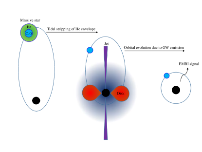
Figure 1: A schematic diagram of the mechanism for observing EMRI and relevant tidal disruption EM signal in our model. Initially, an onion-skin layered massive star orbits an SMBH. After the He envelope gets tidally stripped, X-ray flares are produced by the accretion flow. In some cases, a relativistic jet could be launched by the accreting SMBH. Eventually, the left compact C-O core with density about $10^{6}\text{ g}\text{ cm}^{-3}$ will inspiral into the SMBH and produce EMRI signal in the LISA band.

2 Tidal stripping of stellar envelope and flares

When a star passes close enough through an SMBH, it will be torn apart by the tidal force (Hills, 1975; Rees, 1988; Evans, 1989; Phinney, 1989). A star with density $\rho$ is tidally disrupted when the work exerted over it by the tidal force exceeds its binding energy (Rees, 1988; Amaro-Seoane, 2018). The tidal radius can be calculated from

$$R_{\text{T}}\simeq R_{*}\bigg{(}\frac{M_{\text{BH}}}{M_{*}}\bigg{)}^{1/3}=\bigg{(}\frac{3M_{\text{BH}}}{4\pi\rho}\bigg{)}^{1/3},$$ (1)

where $M_{\text{BH}}$ is the mass of the BH, $R_{*}$ and $M_{*}$ are the stellar radius and stellar mass respectively. The penetration factor $\beta$ defines the strength of the tidal interaction exerted on the star (Carter & Luminet, 1982)

$$\beta=\frac{R_{T}}{R_{p}},$$ (2)

where $R_{p}=a(1-e)$ is the pericenter.

Besides the whole star, the envelopes of evolving stars can also be tidally stripped. For example, the ultraviolet-optical transient PS1-10jh can be explained by tidal disruption of a helium-rich stellar core, which is considered the remnant of a tidally stripped red giant (RG) star (Gezari et al., 2012). Furthermore, Bogdanovic, Cheng & Amaro-Seoane (2014) studied the tidal stripping of an RG star’s envelope by an SMBH and the subsequent inspiral of the core toward the BH. Typically, a massive star has a so-called “onion-skin” structure at the end of its evolution, where each shell has different chemical compositions and mass densities (Woosley, Heger & Weaver, 2002). The outer layers have much lower densities than the core, which makes them more vulnerable to tidal forces. Therefore, a massive star may lose its envelopes partially or completely when it passes close enough through an SMBH, leaving a dense core on a highly eccentric orbit (Di Stefano et al., 2001; Kobayashi et al., 2004; Davies & King, 2005; Amaro-Seoane et al, 2007; Guillochon & Ramirez-Ruiz, 2013). The tidal disruption flares of main sequence stars and helium stars accompanied by GW bursts were investigated previously (Kobayashi et al., 2004). However, this type of GW bursts can not be observed if luminosity distance $d_{L}$ is larger than $20\text{ Mpc}$ (Kobayashi et al., 2004), which limits its cosmological applications.

Here, we propose a new formation channel for EMRIs with EM precursors. In our model, we assume that a massive star has lost H envelope during the red supergiant period. It is in the He burning stage (Heger et al., 2003) and the densities of different layers vary from $10^{0-3}\text{ g}\text{ cm}^{-3}$ (He envelope) to $10^{5-6}\text{ g}\text{ cm}^{-3}$ (carbon-oxygen (C-O) core) (Woosley, Heger & Weaver, 2002). After the He envelope is tidally stripped by the SMBH and the C-O core finally inspirals into the SMBH, we can detect a tidal disruption event (TDE) and the subsequent EMRI signal. For a TDE, we can identify its host galaxy and determine the redshift through spectral lines observation. With the luminosity distance $d_{L}$ from the EMRI signal and the redshift $z$, we have a new type of standard siren. The luminosity distance can be determined to $10\%$ precision at $z=1$. Figure 1 shows a schematic picture of our model.

Since the typical density of He envelope is $10^{3}\text{ g}\text{ cm}^{-3}$ (Woosley, Heger & Weaver, 2002), the tidal stripping should take place in an orbit of semimajor axis $a\sim$ a few $10^{-6}\text{ pc}$ and eccentricity $e=0.90\sim 0.98$. For our scenario to work successfully, the tidal radius of He envelope $R_{\text{T, He}}$ should be larger than the innermost stable circular orbit (ISCO) radius $R_{\text{ISCO}}$. Meanwhile, the tidal radius of C-O core $R_{\text{T,C-O}}$ should be smaller than $R_{\text{ISCO}}$. Therefore, the feasible mass range of centeral SMBH is approximately $3\times 10^{4}\sim 8\times 10^{5}M_{\odot}$.

Below we show the observational properties of the tidal disruption flare in our model. The energy required to strip the stellar envelope is (Davies & King, 2005)

$$E_{\text{strip}}\sim\frac{GM_{c}M_{e}}{R_{c}},$$ (3)

where $M_{c}$, $R_{c}$ and $M_{e}$ are core mass, core radius and stripped envelope mass respectively. If the tidal disruption happens on a highly eccentric orbit, about half of the debris will fall back to the BH, in which case the luminosity of TDE is supposed to follow the standard $t^{-5/3}$ decay rate (Rees, 1988; Evans, 1989; Phinney, 1989). For a 15$M_{\odot}$ star, the masses of the core and stellar debris are about 3 $M_{\odot}$ and 1$M_{\odot}$ respectively. Assuming $f$ is the fraction of the accreted stellar envelope relative to the massive star, then the bound material returns to pericenter at a rate

$$\dot{M} \simeq\frac{1}{3}\frac{fM_{*}}{P_{\text{min}}}\bigg{(}\frac{t}{P_{\text{min}}}\bigg{)}^{-5/3}$$ (4)

$$\simeq 6\times 10^{2}M_{\odot}\text{ yr}^{-1}\bigg{(}\frac{f}{0.25}\bigg{)}$$

$$\cdot\bigg{(}\frac{R_{*}}{10^{10}\text{ cm}}\bigg{)}^{-3/2}\bigg{(}\frac{M_{*}}{4M_{\odot}}\bigg{)}^{2}\bigg{(}\frac{M_{\rm BH}}{10^{5}M_{\odot}}\bigg{)}^{-1/2}\bigg{(}\frac{t}{P_{\text{min}}}\bigg{)}^{-5/3},$$

where

$$P_{\text{min}} =\frac{2\pi R_{p}^{3}}{(GM)^{1/2}(2R_{*})^{3/2}}$$ (5)

$$\simeq 6\times 10^{3}\text{ s}\bigg{(}\frac{R_{*}}{10^{10}\text{ cm}}\bigg{)}^{3/2}\bigg{(}\frac{M_{*}}{4M_{\odot}}\bigg{)}^{-1}M_{5}^{1/2},$$

is the shortest Keplerian orbital period (Ulmer, 1999; Bogdanovic, Cheng & Amaro-Seoane, 2014); $M_{5}$ is defined as $M_{5}\equiv M_{\text{BH}}/(10^{5}M_{\odot})$.

The luminosity of the accretion flow falling back to the SMBH is (Bogdanovic, Cheng & Amaro-Seoane, 2014)

$$L =\epsilon\dot{M}c^{2}$$ (6)

$$\simeq 2\times 10^{48}\text{ erg}\text{ s}^{-1}\bigg{(}\frac{f}{0.25}\bigg{)}\bigg{(}\frac{\epsilon}{0.057}\bigg{)}\bigg{(}\frac{R_{*}}{10^{10}\text{ cm}}\bigg{)}^{-3/2}$$

$$\cdot\bigg{(}\frac{M_{*}}{4M_{\odot}}\bigg{)}^{2}M_{5}^{-1/2}\bigg{(}\frac{t}{P_{\text{min}}}\bigg{)}^{-5/3},$$

where $\epsilon=1-(r-2)/[r(r-3)]^{1/2}$ is the radiative efficiency for a Schwarzschild black hole and $r$ is the orbital radius of the debris in units of $R_{g}$ (Bogdanovic, Cheng & Amaro-Seoane, 2014). The luminosity can be significantly larger than the Eddington limit for a period of weeks to years (Strubbe & Quataert, 2009). When $e\leq e_{\text{crit}}=1-2q^{-1/3}/\beta$ where $\beta\equiv M_{\text{BH}}/M_{*}$, the event is categorized as eccentric TDE (Hayasaki et al., 2018) and all of the debris will remain gravitationally bound to the SMBH. In these cases, the mass fallback rate is flatter and slightly higher than the standard rate (Hayasaki et al., 2018). Besides, the fallback rate and TDE light curve of more centrally concentrated stars show a significant deviation from the $t^{-5/3}$ decay rate (Lodato, King & Pringle, 2009; Hayasaki, Stone & Loeb, 2013; Dai, Escala & Coppi, 2013; Bogdanovic, Cheng & Amaro-Seoane, 2014).

The spectra of tidal flares are very complicated, which are a superposition of blackbody spectrum and many emission lines (Strubbe & Quataert, 2009). The temperature of the debris is

$$T_{\text{eff}}=\bigg{(}\frac{L}{16\pi R_{T}^{2}\sigma}\bigg{)}^{1/4}\simeq 2\times 10^{5}\text{ K}\,M_{5}^{1/12}.$$ (7)

The luminosity $L$ of the X-ray flares from accretion flow falling back to the SMBH is about $10^{48}\text{ erg}\text{ s}^{-1}$ as estimated above. For Einstein Probe under construction, which will have a field of view of 3,600 square degrees, the flux sensitivity can be up to $10^{-10}$ erg cm^-2 s^-1 (Yuan et al., 2015). Hence, Einstein Probe can detect the X-ray flares at $z\geq 1.0$. In some cases, a TDE is accompanied by a relativistic jet, which has been observed in the transient Swift J1644+57 (Bloom et al., 2011; Burrows et al., 2011; Zauderer et al., 2011). If the jet points to us, its luminosity will be much higher than that of the accretion flow.

3 Structure and orbital evolution of the compact core

3.1 Radius expansion after tidal stripping

After the He envelope is stripped, the core has to adjust to a new equilibrium by expanding its radius. For solar-type stars, the core expansion had been extensively discussed using the mass-radius relation for the adiabatic evolution of a nested polytrope (Hjellming & Webbink, 1987; MacLeod et al., 2013; Bogdanovic, Cheng & Amaro-Seoane, 2014). However, MacLeod et al. (2013) showed that the assumptions for the mass-radius relation are incorrect. Therefore, we perform a rough estimation of the new radius using hydrostatic equilibrium equation, the first law of thermodynamics and the relation between pressure and internal energy density instead. The 15 $M_{\odot}$ star’s model of Woosley & Heger (https://2sn.org/stellarevolution/) is used to estimate the pressure in the out layer of the C-O core before expansion. According to Pols (2011), the ideal gas assumption is taken for the He envelope and the C-O core. We find that the core’s radius will increase just 16%, which may not affect the tidal radius greatly.

3.2 Requirements for EMRI formation

In order for a compact object to become an EMRI, its orbital decay timescale by GW emission $\tau_{\text{GW}}$ (Gair, Kennefick & Larson, 2006) should be sufficiently shorter than the two-body relaxation timescale $t_{\text{rlx}}$ (Amaro-Seoane et al, 2007),

$$\tau_{\text{GW}}<C_{\text{EMRI}}(1-e)t_{\text{rlx}}.$$ (8)

where $C_{\text{EMRI}}$ is a numerical constant sufficiently less than 1 and $t_{\text{rlx}}$ is about $10^{9}\text{ yr}$. Otherwise, the compact core will be deflected from its original orbit through two-body relaxation.

There is also a limitation on eccentricity $e$. The maximal eccentricity for a non-plunging orbit is (Cutler, Kennefick & Poisson, 1994; Hopman & Alexander, 2005)

$$e_{\text{max}}(a)=-\frac{R_{\text{S}}}{2a}+\sqrt{\bigg{(}\frac{R_{\text{S}}}{2a}\bigg{)}^{2}-\frac{3R_{\text{S}}}{a}+1},$$ (9)

which is depicted in Figure 2 with green dashed line.

3.3 Time lag between TDE and EMRI signal

Here, we consider the orbital evolution of the C-O core inspiral. It is reasonable to assume that the He envelope is completely stripped after several close encounters. Hence, the interaction between the diffuse envelope and the core can be neglected here (Amaro-Seoane et al, 2007). Furthermore, since $a$ is only a few $10^{-6}\text{ pc}$, the encounters of the compact core with cluster stars around the SMBH are ignored.

The semimajor axis $a$ will shrink due to GW radiation. The Keplerian orbital evolution is given by Peters formalism (Peters, 1964), which is a good approximation in weak-field regime. Apparently, there is an important factor that should be taken seriously—the lag time between the tidal disruption and the EMRI signal. The EMRI enters the LISA band when its frequency $f$, which is twice the Keplerian orbital frequency $f_{\text{orb}}=(GM/4\pi a^{3})^{1/2}$, is larger than $10^{-4}\text{ Hz}$. It was estimated that, for a binary system consisting of a main sequence star and a compact object, the latter will spend $10^{2}$ to $10^{4}$ years to spiral into the SMBH after the main sequence star gets tidally disrupted, which prevents the TDE from being a good precursor to the EMRI (Amaro-Seoane et al, 2007).

However, the situation can be different for a massive star. Its tidal radius is much smaller than that of the main sequence star, which will greatly shorten the time lag between TDE and EMRI. The lag time contour at as a function of initial semi-major axis $a_{0}$ and eccentricity $e_{0}$ is plotted in Figure 2. In the upper left region, the lag time is shorter than 20 years, which is ideal for observing the TDE and subsequent EMRI.

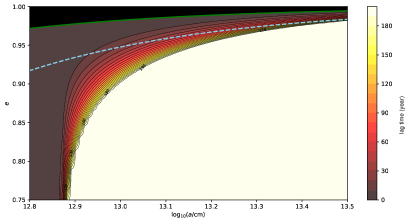
Figure 2: The contour of lag time between TDE and EMRI signal for different initial values of $a_{0}$ and $e_{0}$. The mass of the SMBH is chosen as $3\times 10^{5}M_{\odot}$. The blue dashed line refers to the tidal radius $R_{T}$ where the He envelope (the density is taken to be $10^{3}\text{ g}\text{ cm}^{-3}$) is disrupted. For the upper left brown region, the lag times are less than a decade, which are ideal for observing the TDE and EMRI association. The upper black region represents the direct plunge orbit and the green solid line is the upper limit for non-plunging orbit. For the right bottom region of the diagram, the lag times are all larger than 200 years and are not shown in detail in the contour.

4 Signal-to-noise ratio of EMRI

The number of inspiral cycles in the frequency range [$f_{\text{min}},f_{\text{max}}$] is given by

$$N_{\text{cycles}}=\int_{f_{\text{min}}}^{f_{\text{max}}}\frac{f}{\dot{f}}\mathrm{d}f.$$ (10)

Typically, the small body will spend $10^{4-5}$ cycles inspiralling into the SMBH, being observable for several years before plunge. The characteristic strain $h_{c}$ of the GW from a source emitting at frequency $f$ is (Finn & Thorne, 2000; Barack & Cutler, 2004; Maggiore, 2018; Robson, Cornish & Liu, 2019; Amaro-Seoane, 2018)

$$h_{c}(f)=2f|\tilde{h}(f)|=\bigg{(}\frac{2f^{2}}{\dot{f}}\bigg{)}^{1/2}h_{0}=\frac{(2\dot{E}/\dot{f})^{1/2}}{\pi D},$$ (11)

where $h_{0}$ is the instantaneous root-mean-square amplitude, $\dot{E}$ is the GW emission power and $D$ is the proper distance to the source. In our model, the characteristic strain $h_{c}$ is about $10^{-19}$. It is worth mentioning that a fully coherent search of $10^{4-5}$ cycles for EMRI detection is computationally impossible. The feasible approach is hierarchical matched filtering by dividing data into short data segments (Gair et al., 2004, 2013). The signal-to-noise ratio (S/N) is built up in the second stage of the search by incoherently adding the power of short segments (Gair et al., 2004), which will decreases by a factor $N^{-1/4}$ than a fully coherent search, where $N$ is the number of divided segments (Maggiore, 2018). An incoherent search will be able to detect signals with $S/N\geq 20$; while in a fully coherent search, the S/N required for detection is 12$\sim$14 (Amaro-Seoane et al, 2007; Babak et al., 2017). The S/N can be estimated by (Maggiore, 2018; Robson, Cornish & Liu, 2019)

$$(S/N)^{2}=\int_{f_{1}}^{f_{2}}\frac{h_{c}^{2}(f)}{h_{n}^{2}(f)}\mathrm{d}(\ln f),$$ (12)

where $h_{n}^{2}(f)=fS_{n}(f)$ and $S_{n}(f)$ is the noise spectral density of the detector (Maggiore, 2018). In our analysis, a S/N threshold of 36 is assumed for incoherent search. Then EMRIs formed in our channel can be detected as far as $z\sim 1$ (about 3.4 Gpc). The foreground noise from white dwarf binaries affects the detection of EMRIs, which has been discussed by many authors (Cornish & Larson, 2003; Farmer & Phinney, 2003). Some algorithms are used to subtract this noise (Cornish & Larson, 2003) but their performances are rather uncertain. However, even assume a 30% decrease of S/N after subtracting the WD background, the detection range will not be less than $z\sim 0.7$. The schematic diagram of EMRI’s characteristic strain $h_{c}$ as a function of $f$ is shown in Figure 3. The LISA’s sensitivity curve is generated from the online sensitivity curve generator$\--$see Larson (2003).

By the way, the mass loss of the C-O core due to tidal stripping after entering LISA band is less than 20%, which may not affect the detection of EMRI.

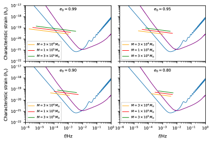
Figure 3: The diagram of EMRI’s characteristic strain $h_{c}$ as a function of GW frequency $f$. For comparison, the sensitivity curves of LISA and Tianqin are plotted with blue and purple lines respectively. Each panel is depicted with a certain initial orbit eccentricity $e_{0}$ and different black hole masses. The mass of the C-O core is 3$M_{\odot}$ and the redshift of the EMRI system is $z=0.2$ for all panels.

5 Event rate

In order to estimate the rate of EMRIs occurring in the universe, two ingredients must be considered. The first is the spatial density of SMBHs in the appropriate mass range. The second is the rate at which each black hole tidally disrupts massive stars. From observations, the space density of SMBHs can be approximated by $M_{\rm BH}-\sigma$ relation

$$M_{\rm BH}=M_{\rm BH,*}\,\,\left(\frac{\sigma}{\sigma_{*}}\right)^{\lambda},$$ (13)

where $\sigma$ is the spheroid velocity dispersion. We use $\sigma_{*}=90\,{\rm km\,s^{-1}}$, $\lambda=4.72$ and $M_{\rm BH,*}=3\times 10^{6}\,M_{\odot}$ (Merritt & Ferrarese, 2001). The above relation is derived from SMBHs with masses ranging from $10^{6}$ to $10^{9}$ $M_{\odot}$. For low-mass SMBHs ($<10^{6}M_{\odot}$), Xiao et al. (2011) found that the $M_{\rm BH}-\sigma$ relation is consistent with the above relation allowing for the uncertainties. Therefore, the $M_{\rm BH}-\sigma$ in equation (13) is used in our derivation. The galaxy velocity dispersion function is constrained using galaxy luminosity functions and $L\--\sigma$ correlation (Aller & Richstone, 2002). Combined with the $M_{\rm BH}\--\sigma$ relation, the black hole mass function is (Gair et al., 2004)

$$M_{\rm BH}\,\frac{\mathrm{d}N}{\mathrm{d}M_{\rm BH}}=\phi_{*}\,\frac{\epsilon}{\Gamma\left(\frac{\gamma}{\epsilon}\right)}\,\left(\frac{M_{\rm BH}}{M_{\rm BH,*}}\right)^{\gamma}\,\exp\left[-\left(\frac{M_{\rm BH}}{M_{\rm BH,*}}\right)^{\epsilon}\right],$$ (14)

where $\epsilon=3.08/\lambda$, $\phi_{*}$ is the total number density of galaxies, and $\Gamma(z)$ is the Gamma function. Aller & Richstone (2002) derived the parameters $\phi_{*}$, $M_{\rm BH,*}$ and $\gamma$ for different types of galaxies. For the mass range of interest in this analysis, $M_{\rm BH}<10^{6}M_{\odot}$, the parameters are $\phi_{*}=36.7~{}h_{70}^{2}\,{\rm Mpc}^{-3}$, $M_{\rm BH,*}=4\times 10^{6}M_{\odot}$ and $\gamma=0.03$. The spatial density of black holes is approximately

$$M_{\rm BH}\,\frac{\mathrm{d}N}{\mathrm{d}M_{\rm BH}}=2\times 10^{-3}\,h_{70}^{2}\,{\rm Mpc}^{-3},$$ (15)

where $h_{70}\equiv H_{0}/70\,{\rm km\,s^{-1}\,Mpc^{-1}}$ is the dimensionless Hubble parameter.

The rate at which each SMBH disrupts massive stars can be calculated using the loss cone theory (Magorrian & Tremaine, 1999; Wang & Merritt, 2004). For solar-type stars, the disruption rate per galaxy is (Wang & Merritt, 2004)

$$\mathcal{R}=6.5\times 10^{-4}\text{ yr}^{-1}\left(\frac{M_{*}}{M_{\odot}}\right)^{-1/3}\left(\frac{R_{*}}{R_{\odot}}\right)^{1/4}\left(\frac{M_{\text{BH}}}{10^{6}M_{\odot}}\right)^{-1/4}.$$ (16)

Using the standard Salpeter initial mass function, the number ratio of 15-40$M_{\odot}$ stars to solar-type stars is $1.4\times 10^{-2}$. The lifetime ratio of massive star with 15$M_{\odot}$ to solar type star is about $10^{-3}$. In addition, the typical density of the He envelope is $10^{3}$ times larger than that of solar-type star, so the tidal radius is one order of magnitude smaller. Hence, the rate should be lowered by another factor of $10^{-3}$. What’s more, for our scenario to work, it is required that the star is on the He main sequence, whose duration lasts roughly 0.1 times that of the H main sequence. Combining all of the above factors and integrating equation (15) over $15\,M_{\odot}<M_{*}<40\,M_{\odot}$, $0.2R_{\odot}<R_{*}<8R_{\odot}$, the event rate is $2\times 10^{-4}~{}\rm Gpc^{-3}yr^{-1}$ for $M_{\text{BH}}=5\times 10^{5}M_{\odot}$.

Below, we briefly discuss how to identify this type of EMRIs. From the spectrum of flare, the redshift of tidal stripping event can be measured and the host galaxy can be localized. After a few tens of years, LISA may detect EMRI signal in the same direction, which will determine the sky location to a few square degrees and the luminosity distance to 10% precision (Babak et al., 2017). Combing the redshift information from the flare with host galaxy properties, we can determine whether the flare and the EMRI occur in the same galaxy.

6 Summary

EMRI is a promising tool to study the strong field gravity, the stellar dynamics in galactic nuclei, massive black hole populations (Babak et al., 2017; Amaro-Seoane, 2018) and many other aspects of astrophysics. In this paper, we propose a new formation channel for EMRIs, in which the tidal disruption flares can serve as EM precursor. The event rate of this type of EMRIs is about $2\times 10^{-4}~{}\rm Gpc^{-3}\text{ yr}^{-1}$. Combined with relevant EM signals, EMRIs will serve as a new standard siren to probe the expansion of universe.

References

- Abbott et al. (2017a) Abbott, B. P., et al. (LIGO Scientific Collaboration and Virgo Collaboration) 2017, Phys. Rev. Lett., 119, 161101
- Abbott et al. (2017b) Abbott, B. P. et al. (LIGO Scientific Collaboration and Virgo Collaboration) 2017, Nature, 551, 85
- Aller & Richstone (2002) Aller, M. C., & Richstone, D. 2002, AJ, 124, 3035
- Amaro-Seoane et al (2007) Amaro-Seoane, P., et al. 2017 Class. Quantum Grav., 24, R113
- Amaro-Seoane et al (2017) Amaro-Seoane, P., et al. arXiv: 1702.00786
- Amaro-Seoane (2018) Amaro-Seoane, P. 2018, Living Rev Relativ, 21, 4
- Babak et al. (2017) Babak, S., et al. 2017, Phys. Rev. D, 95, 103012
- Barack & Cutler (2004) Barack, L. & Cutler, C. 2004, Phys. Rev. D, 69, 082005
- Bloom et al. (2011) Bloom, J. S. et al. 2011, Science, 333, 203
- Bogdanovic, Cheng & Amaro-Seoane (2014) Bogdanovi, T., Cheng, R. M., & Amaro-Seoane, P. 2014, ApJ, 788, 99
- Burrows et al. (2011) Burrows, D. N., et al. 2011, Nature, 476, 421
- Carter & Luminet (1982) Carter, B., & Luminet, J. P. 1982, Nature, 296, 211
- Chen, Fishbach & Holz (2018) Chen, H. Y., Fishbach, M., & Holz, D. E. 2018, Nature, 562, 545
- Cornish & Larson (2003) Cornish, N. J., & Larson, S. L. 2003, Phys. Rev. D, 67, 103001
- Cutler, Kennefick & Poisson (1994) Cutler, C., Kennefick, D., & Poisson, E. 1994, Phys. Rev. D, 50, 6
- Cutler (1998) Cutler, C. 1998, Phys. Rev. D, 57, 12
- Dai, Escala & Coppi (2013) Dai, L. X., Escala, A., & Coppi, P. 2013, ApJ, 775, L9
- Danzmann et al. (2000) Danzmann, K. et al. 2000, Adv. Space Res., 25, 1129
- Davies & King (2005) Davies, M. B., & King, A. 2005, ApJ, 624, L25
- Di Stefano et al. (2001) Di Stefano, R., et al. 2001, ApJ, 551, L37
- Evans (1989) Evans, C. R., & Kochanek, C. S. 1989, ApJ, 346, L13
- Farmer & Phinney (2003) Farmer, A. J., & Phinney, E. S. 2003, MNRAS, 346, 1197
- Finn & Thorne (2000) Finn, L. S. & Thorne, K. S. 2000, Phys. Rev. D, 62, 124021
- Gair et al. (2004) Gair, J. R., et al. 2004, Class. Quantum Grav., 21, S1595
- Gair, Kennefick & Larson (2006) Gair, J. R. Kennefick, D. J., & Larson, S. L. 2006, ApJ, 639, 999
- Gair et al. (2013) Gair, J. R., et al. 2013, Living Rev Relativ, 16, 7
- Gezari et al. (2012) Gezari, S., et al. 2012, Nature, 485, 217
- Guillochon & Ramirez-Ruiz (2013) Guillochon, J., & Ramirez-Ruiz, E. 2013, ApJ, 767, 25
- Hannuksela et al. (2019) Hannuksela, O. A., Wong, K. W. K., Brito, R., Berti, E., & Li, T. G. F. 2019, Nat. Astron., 3, 447
- Hayasaki et al. (2018) Hayasaki, K., Zhong, S. Y., Li, S., Berczik, P., & Spurzem, R. 2018, ApJ, 855, 129
- Hayasaki, Stone & Loeb (2013) Hayasaki, K., Stone, N., & Loeb. A. 2013, MNRAS, 434, 909
- Heger et al. (2003) Heger, A., Fryer, C. L., Woosley, S. E., Langer, N., & Hartmann, D. H. 2003, ApJ, 591, 288
- Hills (1975) Hills, J. G. 1975, Nature, 254, 295
- Hjellming & Webbink (1987) Hjellming, M. S., & Webbink, R. F. 1987, ApJ, 318, 794
- Hopman & Alexander (2005) Hopman, C., & Alexander, T. 2005, ApJ, 629, 362
- Hu & Wu (2017) Hu, W. R., & Wu, Y. L. 2017, Natl Sci Rev, 4, 5
- Kobayashi et al. (2004) Kobayashi, S., Laguna, P., Phinney, E. S., & Mészáros, P. 2004, ApJ, 615, 855
- Larson (2003) Larson, S. L. Online sensitivity curve generator. http://www.srl.caltech.edu/ shane/sensitivity/MakeCurve.html
- Lodato, King & Pringle (2009) Lodato, G. King, A. R. & Pringle, J. E. 2009, MNRAS, 392, 332
- Lodato & Rossi (2011) Lodato, G., & Rossi, E. M. 2011, MNRAS, 410, 359
- Luo et al. (2015) Luo, J., et al. 2016, CQGra, 33, 035010
- MacLeod et al. (2013) MacLeod, M., Ramirez-Ruiz, E., Grady, S., & Guillochon, J. 2013, ApJ, 777, 133
- Merritt et al. (2011) Merritt, D., Alexander, T., Mikkola, S., & Will, C. M. 2011, Phys. Rev. D, 84, 044024
- Merritt & Ferrarese (2001) Merritt, D., & Ferrarese, L. 2001, ApJ, 547, 140
- Magorrian & Tremaine (1999) Magorrian, J., & Tremaine, S. 1999, MNRAS, 309, 447
- Maggiore (2018) Maggiore, M. 2018, Gravitational Waves, Volume 2 Astrophysics and Cosmology, Oxford University Press
- Peters (1964) Peters, P. C. 1964, Phys. Rev., 136, 4B
- Phinney (1989) Phinney, E. S. 1989, IAU Symp. 136, The Center of the Galaxy, ed. M. Morris (Dordrecht: Kluwer Academic Publishers), 543
- Phinney (2002) Phinney, E. S. 2002, LISA science requirements
- Pols (2011) Pols, O. R. 2011, Stellar Structure and Evolution
- Rees (1988) Rees, M. J. 1988, Nature, 333, 523
- Robson, Cornish & Liu (2019) Robson, T., Cornish, N. J., & Liu, C. 2019, Class. Quantum Grav., 36 105011
- Sigurdsson & Rees (1997) Sigurdsson, S., & Rees, M. J. 1997, MNRAS, 284, 318
- Strubbe & Quataert (2009) Strubbe, L. E., & Quataert, E. 2009, MNRAS, 400, 2070
- Ulmer (1999) Ulmer, A. 1999. ApJ, 514, 180
- Wang & Merritt (2004) Wang, J., & Merritt, D. 2004, ApJ, 600, 149
- Wang & Wang (2019) Wang, Y. Y., & Wang, F. Y. 2019, ApJ, 873, 39
- Wang, Wang & Zou (2018) Wang, Y. Y., Wang, F. Y. & Zou, Y. C., 2018, PRD, 98, 063503
- Woosley, Heger & Weaver (2002) Woosley, S. E., Heger, A., & Weaver, T. A. 2002, \rmp, 74, 1015
- Xiao et al. (2011) Xiao, T., et al., ApJ, 739, 28
- Yuan et al. (2015) Yuan, W., et al. arXiv:1506.07735
- Zauderer et al. (2011) Zauderer, B. A., et al. 2011, Nature, 476, 425