Radiative corrections in proton–antiproton annihilation to electron-positron and their application to the PANDA experiment

Abstract

Radiative corrections to the annihilation of proton–antiproton into electron–positron are revisited, including virtual and real (soft and hard) photon emission. This issue is relevant for the time-like form factors measurements planned at the PANDA experiment at the FAIR facility, in next future. The relevant formulas are given. A stand-alone Monte-Carlo integrator is developed on the basis of the calculated radiative cross section and its application to the PANDA experiment is illustrated.

1 Introduction

The elementary annihilation process $\bar{p}+p\to e^{+}+e^{-}$ and the time-reverse reaction $e^{+}+e^{-}\to\bar{p}+p$ contain direct information on the proton electromagnetic form factors (FFs). FFs are fundamental quantities that conveniently parametrize the electric and magnetic currents in the proton. The kinematical region accessed by annihilation reactions is the time-like (TL) region of transferred momenta $q^{2}$, where $q^{2}$ is positive. Assuming that the reactions occur through the exchange of a virtual photon of four momentum squared $q^{2}$, the annihilation cross section is parametrized in terms of two complex amplitudes, that are functions of $q^{2}$ only. At the leading order in the fine electromagnetic constant, $\alpha=e^{2}/4\pi\approx 1/137$, (Born approximation), the cross section contains the moduli squared of FFs, and shows a linear dependence in $\cos^{2}\theta$, where $\theta$ is the angle of the produced electron in the center of mass system (c.m.s). The precise measurement of the angular distribution of one of the final particles allows to access directly the electric and magnetic FFs [1].

However, the charged particles involved in the reaction irradiate and the emission of real or virtual photons requires higher order corrections to the measured cross section in order to recover the Born cross section (Fig. 1) and extract TL FFs.

Extensive literature is dedicated to radiative corrections to electron proton scattering (for a recent review see [2]), few works were previously dedicated to this physics issue in the context of the physics program of the PANDA [3] experiment at FAIR [4]. In space-like (SL) region updated radiative corrections calculations were made necessary by the program of FF measurements at the Jefferson Laboratory, at large transferred momentum. Following the Akhiezer–Rekalo polarization method [5, 6], the GEp collaboration measured precisely the ratio of the electric $G_{E}$ to magnetic $G_{M}$ FFs in a series of experiments [7] and found a large deviation from unity, contrary to what previously suggested by unpolarized cross section measurements, using the Rosenbluth method [8].

Among the possible explanations of this discrepancy: normalization issues in the data [9], correlations in the parameters of the Rosenbluth fit [10], radiative corrections at higher orders [11] or more precise first order corrections [12], the community largely focussed on a possible enhancement of the two photon exchange mechanism [13]. Model dependent calculations showed that a large effect increasing with $Q^{2}=-q^{2}$ could be indeed found [14, 15]. An exact calculation is not feasible, because one should know the $Q^{2}$ dependence of the FFs for all intermediate proton excited states. Model independent considerations, however, predict that the two photon contribution introduces charge odd terms, that are sources of non-linearities in the Rosenbluth plots, in SL region, and of odd powers of $\cos\theta$ terms in TL region. As for today, no experimental evidence of enhancement of the two photon exchange contribution has been found (for a recent discussion, see [16]. The importance of this issue is related to the fact that, in presence of multi-photon exchange, the formalism that relates the observables to FFs does not hold any more. Instead of two real FFs, function of $Q^{2}$, the scattering process would be described by three amplitudes in general complex functions of two kinematical variables [17, 18]. It would be still possible to extract the real FFs, functions of $Q^{2}$ but at the price of difficult measurements of polarization observables, including double and triple polarizations, of the order of $\alpha$. Attention should be given to this problem, because even a few percent relative contribution of the two photon mechanism, would bring when neglected large inconsistencies in the FFs extraction. In the TL region, the two photon exchange contribution could be easier to be measured. Having a precise angular distribution, the sum (difference) of the differential cross section at complementary angles cancels (enhances) the charge odd contributions. The sum of cross sections for $\theta$ and $\pi-\theta$ would still be an even function of $\cos\theta$, and of $G_{E,M}^{2}\left(Q^{2}\right)$ [19, 20].

In the TL domain, precise radiative corrections have been implemented for experiment at electron-positron colliders at LEP and more recently for BESIII [21, 22]. The necessary high precision is obtained with Monte-Carlo based on the lepton Structure Function method [23] that allows to take into account higher orders in the leading logarithmic approximation.

The feasibility studies for the measurement of the $\bar{p}p\to e^{+}e^{-}$ process have been performed [24], and more recently within the PANDARoot framework [25], at the different energies accessible by the PANDA experiment. The expected precision on the measurements of $\left|G_{E}\right|$, $\left|G_{M}\right|$, and on their ratio $R$ were evaluated, assuming an integrated luminosity of $2\leavevmode\nobreak\ \mbox{fb}^{-1}$ per beam momentum setting. The results of the simulations show that the proton form factor ratio can be measured with a total relative uncertainty between $3.3\%$ at $s=5.08\leavevmode\nobreak\ \mbox{GeV}^{2}$ and $57\%$ at $s=13.9\leavevmode\nobreak\ \mbox{GeV}^{2}$, including both statistical and systematical uncertainties. The relative uncertainty on $\left|G_{E}\right|$ ($\left|G_{M}\right|$) is between $2.2\%$ ($3.5\%$) and $48\%$ ($9.7\%$). The measurement of total cross section, that gives an effective form factor, can be in principle extended to higher energy values ($\sim 40\leavevmode\nobreak\ \mbox{GeV}^{2}$) depending on the real experimental efficiency.

The PANDARoot analysis program includes the package PHOTOS [26] for the calculation of radiative corrections, which are not specific to the annihilation reaction $\bar{p}+p\to e^{+}+e^{-}$. In particular the odd effects that may arise from initial (ISR) and final (FSR) state radiation interference (INT) are not taken into account. These effects may induce large errors, if neglected, for the extraction of FFs, as they destroy the symmetry of the angular distribution. Monte-Carlo simulations indicate that the precision of the FFs measurement at PANDA will be of the order of few percent in the near threshold region, becoming larger at larger energy [24, 25]. Therefore it is necessary to quantify high order effect although first order calculations seem sufficient at this stage to be implemented in the data analysis. Radiative corrections (RC) due to the emission of real and virtual photons do affect the measurement of the experimentally observable quantities, in particular the differential cross section. The individual determination of the electric and magnetic proton FFs requires the precise knowledge of the angular distribution of the final lepton, in shape and in absolute value.

The motivation of this paper is to derive and collect the relevant formulas for soft and hard photon emission in $\bar{p}+p\to e^{+}+e^{-}$ in a convenient form to be implemented in a stand-alone Monte-Carlo integrator and to compare the results of the simulations with previous calculations.

The paper is organized as follows: Section 2 gives the notations of the four momenta and the definitions and formulas for the Born cross section. Section 3 contains the evaluation of different radiative contributions to the process. These contributions are presented in the corresponding subsections: subsections 3.1 and 3.2 give the expressions for virtual radiative corrections and for soft real photon emission contribution to the Born diagram and compares to the existing calculations, while subsection 3.3 is devoted to the hard photon emission overview. Section 4 gives the results in form of tables and figures, proving the stability of the numbers with respect to the relevant parameters. And in Section 5 one can find our conclusion on the result obtained.

2 Born cross section

Figure 1: Feynman diagram for the process (1) at tree (Born) level.

The basic process is

$$p(p_{1})+\bar{p}(p_{2})\to e^{+}(k_{1})+e^{-}(k_{2}),$$ (1)

where the particle four-momenta are indicated in parentheses. It is illustrated in Fig. 1. The masses of particles are denoted in the following way: $M$ is mass of proton ($p_{1}^{2}=p_{2}^{2}=M^{2}$) and $m$ is mass of electron ($k_{1}^{2}=k_{2}^{2}=m^{2}$). The velocityies of the proton, electron and any fermion $f$ with mass $m_{f}$ are:

$$\beta_{p}=\sqrt{1-\frac{4M^{2}}{s}},\ \beta_{e}=\sqrt{1-\frac{4m^{2}}{s}},\ \beta_{f}=\sqrt{1-\frac{4m_{f}^{2}}{s}}.$$ (2)

In the kinematical conditions of PANDA the electron mass $m$ can be neglected (i.e., $k_{1}^{2}=k_{2}^{2}=0$ is set everywhere possible), then $\beta_{e}\to 1$, but the proton mass $M$ can not be neglected, therefore, for simplicity, the index $p$ in the definition of $\beta_{p}$ is neglected and $\beta_{p}$ is replaced with the notation $\beta\equiv\beta_{p}$ in all formulas below.

The relativistic kinematics of process (1) is described in terms of Mandelstam invariants:

$$s =\left(p_{1}+p_{2}\right)^{2}=2M\left(M+E\right),$$ (3)

$$t =\left(p_{2}-k_{2}\right)^{2}=-\frac{s}{4}\left(1+\beta^{2}-2\beta\cos\theta\right),$$ (4)

$$u =\left(p_{1}-k_{2}\right)^{2}=-\frac{s}{4}\left(1+\beta^{2}+2\beta\cos\theta\right),$$ (5)

where $\theta$ is the scattering angle between the directions of the antiproton beam and of the final electron ${\bf k_{2}}$ in the c.m.s of initial particles, $E=\sqrt{M^{2}+P^{2}}$ ($P=\left|{\bf p_{2}}\right|$) is the energy(momentum) of the antiproton in the laboratory (Lab) frame (for the proton target: $\vec{p}_{1}=0$). The antiproton beam momentum range in PANDA is $P=1.5\div 15$ GeV. The following relation holds:

$$s+t+u=2m^{2}+2M^{2}\approx 2M^{2},$$ (6)

based on the 4-momentum conservation. In the Born approximation and in c.m.s. of the initial $p\bar{p}$-pair the differential cross section has the form [1]:

$$\sigma_{B}\equiv\frac{d\sigma_{B}}{d\Omega_{-}} = \frac{\alpha^{2}}{4s\beta}\Bigl{[}\left|G_{M}(s)\right|^{2}\left(1+\cos^{2}\theta\right)+$$

$$\left(1-\beta^{2}\right)\left|G_{E}(s)\right|^{2}\sin^{2}\theta\Bigr{]},$$

where the electric $G_{E}$ and the magnetic $G_{M}$ Sachs FFs of the proton [27] are related to the Dirac and Pauli form factors $F_{1,2}$ by:

$$G_{E}(q^{2}) =F_{1}(q^{2})+\tau F_{2}(q^{2}),$$

$$G_{M}(q^{2}) =F_{1}(q^{2})+F_{2}(q^{2}),$$ (8)

where $\tau=q^{2}/4M^{2}$. The four momentum transfer at the proton vertex at the Born level is

$$q=p_{1}+p_{2},\qquad q^{2}=s.$$ (9)

At zero momentum transfer the electric and magnetic form factors are normalized respectively to the charge and to the magnetic moment $\mu_{p}=2.79$ of the proton expressed in nuclear magnetons, i.e., $G_{E}(0)=1$, $G_{M}(0)=\mu_{p}$ and, correspondingly, the Dirac and Pauli form factors are $F_{1}(0)=1$, $F_{2}(0)=\mu_{p}-1$. In the assumption of a point-like proton one has:

$$G_{E}(q^{2})=G_{M}(q^{2})=1,\ \mbox{or}\ F_{1}(q^{2})=1,\ F_{2}(q^{2})=0,$$ (10)

and the Born cross section then reads as:

$$\sigma_{B}^{0}\equiv\frac{d\sigma_{B}^{0}}{d\Omega_{-}}=\frac{\alpha^{2}}{4s\beta}\left(2-\beta^{2}\sin^{2}\theta\right).$$ (11)

Different models and parametrizations exist for the nucleon form factors. We will use either a modified dipole parametrization:

$$G_{E}(q^{2}) =\frac{M_{0}^{4}}{(q^{2}+M_{0}^{2})^{2}},$$ (12)

$$G_{M}(q^{2}) =\mu_{p}\,G_{E}(q^{2}),$$ (13)

where $M_{0}^{2}=0.71\leavevmode\nobreak\ \mbox{GeV}^{2}$ or the vector dominance model extended to the TL region from [28].

The Born cross section depends on FFs, which parametrization have in general been fitted on the existing data. It turns out that the results of radiative corrections depend very weakly on the FF model.

3 Radiative corrections

The radiative corrections to the process (1) at the next to leading order in $\alpha$ include virtual photon emission such as vertex corrections, vacuum loops and the exchange of two photons, as well as real photon emission, from initial and final states, and their interferences. The total amplitude ${\cal M}_{tot}$ is the incoherent sum of the amplitudes for the two different final states: $e^{+}+e^{-}$ including the Born diagram ${\cal M}_{B}$ and the virtual corrections ${\cal M}_{V}$, and $e^{+}+e^{-}+\gamma$ describing the real photon emission ${\cal M}_{\gamma}$ in the initial (ISR) and final (FSR) states:

$$\sigma \sim \left|{\cal M}_{tot}\right|^{2}=\left|{\cal M}_{B}+{\cal M}_{V}\right|^{2}+\left|{\cal M}_{\gamma}\right|^{2}$$ (14)

$$= \left|{\cal M}_{B}\right|^{2}+2\,\mbox{Re}\left({\cal M}_{B}^{+}\,{\cal M}_{V}\right)+\left|{\cal M}_{V}\right|^{2}+\left|{\cal M}_{\gamma}\right|^{2},$$

where the amplitudes ${\cal M}_{V}$ and ${\cal M}_{\gamma}$ contain the following contributions:

$${\cal M}_{V} ={\cal M}_{VP}+{\cal M}_{ver}^{e}+{\cal M}_{ver}^{p}+{\cal M}_{box},$$ (15)

$${\cal M}_{\gamma} ={\cal M}_{ISR}+{\cal M}_{FSR}.$$ (16)

Considering the contributions of the order of $\alpha^{3}$ we can write:

$$\sigma \sim \left|{\cal M}_{B}\right|^{2}+2\,\mbox{Re}\left({\cal M}_{B}^{+}\,{\cal M}_{V}\right)+\left|{\cal M}_{\gamma}\right|^{2}$$ (17)

$$= \left|{\cal M}_{B}\right|^{2}\left[1+\frac{2\,\mbox{Re}\left({\cal M}_{B}^{+}\,{\cal M}_{V}\right)}{\left|{\cal M}_{B}\right|^{2}}+\frac{\left|{\cal M}_{\gamma}\right|^{2}}{\left|{\cal M}_{B}\right|^{2}}\right].$$

Therefore cross section with radiative effects of order $\alpha^{3}$ can be written as:

$$\sigma=\sigma_{B}\left(1+\delta_{V}+\delta_{\gamma}\right).$$ (18)

3.1 Virtual photon contributions

The one-loop virtual photon contributions have been calculated in the literature (see, for example [29]). We recall all of them for completeness here. In this section we use the point-like proton approximation, Eq. (10). The total one-loop virtual corrections include the decomposition (15) of the virtual corrections amplitude:

1. the boson self energies (or vacuum polarization), i.e., ${\cal M}_{VP}$,

2. the corrections to proton (${\cal M}_{ver}^{p}$) and electron (${\cal M}_{ver}^{e}$) vertices,

3. the two-photon exchange or box-type contributions, ${\cal M}_{box}$.

Below we present all these contributions separately.

3.1.1 Boson self-energy

Figure 2: Vacuum polarization radiative corrections.

= +

Figure 3: Contributions to the boson self energy operator.

The boson self-energy contribution corresponds to the diagram shown in Fig. 2 where the vacuum polarization operator $\Pi(s)$ has the following terms (see Fig. 3):

$$\Pi(s)=\Pi_{e}(s)+\Pi_{\mu}(s)+\Pi_{\tau}(s)+\Pi_{\rm hadr}(s),$$ (19)

where

$$\Pi_{e}(s) = \frac{\alpha}{3\pi}\left(L_{e}-\frac{5}{3}\right)-i\frac{\alpha}{3},$$ (20)

$$\Pi_{\mu}(s) = -\frac{\alpha}{\pi}\left[\frac{8}{9}-\frac{\beta_{\mu}^{2}}{3}-\frac{\beta_{\mu}}{2}\left(1-\frac{\beta_{\mu}^{2}}{3}\right)L_{\mu}\right]$$ (21)

$$-i\frac{\alpha}{2}\left(1-\frac{\beta_{\mu}^{2}}{3}\right),$$

where we use the following notations for the logarithms:

$$L_{e}\equiv\ln\frac{s}{m^{2}},\qquad L_{\mu}\equiv\ln\frac{1+\beta_{\mu}}{1-\beta_{\mu}}.$$ (22)

The $\tau$-lepton contribution $\Pi_{\tau}$ can be found by substitution $\Pi_{\tau}(s)=\Pi_{\mu}(s)|_{\mu\rightarrow\tau}$. To evaluate the hadronic contribution we consider the charged pion loop contribution:

$$\Pi_{\rm hadr}(s) \approx \Pi_{\pi^{+}\pi^{-}}(s)=\frac{2\alpha}{\pi}\left(\frac{1}{12}L_{\pi}-\frac{2}{3}-2\beta_{\pi}^{2}-i\frac{\beta_{\pi}^{3}}{12}\right),$$ (23)

$$L_{\pi}\equiv\ln\frac{1+\beta_{\pi}}{1-\beta_{\pi}},\ \beta_{\pi}=\sqrt{1-\frac{4m_{\pi}^{2}}{s}}.$$

3.1.2 Vertex corrections

Figure 4: Vertex radiative corrections.

The vertex corrections correspond to the diagrams shown in Fig. 4 where the proton and electron vertices are modified by additional virtual photon exchanges. This contribution leads to the following modification of proton and electron FFs of the order $\alpha$ with respect to the Born level contributions (10):

$$F_{1}(q^{2}) =1+\frac{\alpha}{\pi}F_{1}^{(2)}(q^{2}),$$

$$F_{2}(q^{2}) =\frac{\alpha}{\pi}F_{2}^{(2)}(q^{2}),$$ (24)

$$F_{e}(q^{2}) =1+\frac{\alpha}{\pi}F_{e}^{(2)}(q^{2}),$$

where the functions $F_{i}^{(2)}$ are given below. The modification of proton vertex then reads as:

$$\mbox{Re}\,F_{1}^{(2)} = \left(\ln\frac{M}{\lambda}-1\right)\left(1-\frac{1+\beta^{2}}{2\beta}L_{\beta}\right)+$$

$$\frac{1+\beta^{2}}{2\beta}\left[\frac{\pi^{2}}{3}+\mbox{Li}_{2}\!\left(\frac{1-\beta}{1+\beta}\right)-\frac{L^{2}_{\beta}}{4}-\right.$$

$$\left.L_{\beta}\ln\frac{2\beta}{1+\beta}\right]-\frac{L_{\beta}}{4\beta},\mbox{Re}\,F_{2}^{(2)}$$

$$= -\frac{1-\beta^{2}}{4\beta}L_{\beta},\ L_{\beta}\equiv\ln\frac{1+\beta}{1-\beta}.$$ (26)

This contribution is infrared divergent and is regularized by introducing a fictitious photon mass $\lambda$ which cancels with the soft real photon emission contribution according to the procedure described in [30].

The electron vertex modification leads to

$$\mbox{Re}\,F_{e}^{(2)}=\left(\ln\frac{m}{\lambda}-1\right)\left(1-L_{e}\right)-\frac{L_{e}^{2}}{4}-\frac{L_{e}}{4}+\frac{\pi^{2}}{3}.$$ (27)

3.1.3 Box-type corrections

Figure 5: Box-type radiative corrections.

The box-type contributions are illustrated by the diagrams presented in Fig. 5 and implement two virtual photons exchange mechanism. The box-type contributions are illustrated by the diagrams in Fig. 5 and describe the exchange of two virtual photons. The interference of the box amplitude ${\cal M}_{box}$ (15) with the Born amplitude ${\cal M}_{B}$ (17) is expressed through the following function:

$$I (s,t,u)=(u-t)$$ (28)

$$\left[\left(\frac{2M^{2}}{\beta^{2}}+t+u\right)I_{0qp}-\frac{\pi^{2}}{6}+\frac{1}{2}L_{\beta}^{2}-\frac{1}{\beta^{2}}L_{\beta}\right]+$$

$$(2t+s)\left[\frac{1}{2}L_{ts}^{2}-\mbox{Li}_{2}\!\left(\frac{-t}{M^{2}-t}\right)\right]-$$

$$(2u+s)\left[\frac{1}{2}L_{us}^{2}-\mbox{Li}_{2}\!\left(\frac{-u}{M^{2}-u}\right)\right]+$$

$$[ut-M^{2}(s+M^{2})]\left(\frac{1}{t}L_{ts}-\frac{1}{u}L_{us}+\frac{u-t}{ut}L_{s}\right)+$$

$$I_{0}L_{tu}\left(L_{M\lambda}+L_{s}\right),$$

where

$$I_{0qp} = \frac{1}{s\beta}\Biggl{[}L_{s}L_{\beta}-\frac{1}{2}L_{\beta}^{2}-\frac{\pi^{2}}{6}+2\mbox{Li}_{2}\!\left(\frac{1+\beta}{2}\right)$$ (29)

$$-2\mbox{Li}_{2}\!\left(\frac{1-\beta}{2}\right)-2\mbox{Li}_{2}\!\left(\frac{\beta-1}{\beta+1}\right)\Biggr{]}$$

and for the logarithms we use the following notations:

$$L_{ts} \equiv \ln\frac{M^{2}-t}{s},\ L_{us}\equiv\ln\frac{M^{2}-u}{s},\ L_{s}\equiv\ln\frac{s}{M^{2}},$$ (30)

$$L_{tu}\equiv\ln\frac{M^{2}-t}{M^{2}-u},\ L_{M\lambda}\equiv\ln\frac{M^{2}}{\lambda^{2}}.$$

It is worth to be noted that the coefficient in front of $L_{M\lambda}$ in (28)

$$I_{0}=\frac{2}{s}\left(t^{2}+u^{2}-4M^{2}(t+u)+6M^{4}\right)=s\left(2-\beta^{2}\sin^{2}\theta\right)$$ (31)

is proportional to the modulus squared of the Born amplitude.

3.1.4 Total virtual corrections

Summing the Born contribution and all virtual corrections presented above the differential cross section can be written in the form:

$$\sigma_{BV} = \frac{\alpha^{2}}{4s\beta}\left(2-\beta^{2}\sin^{2}\theta\right)\left|\frac{1}{1-\Pi(s)}\right|^{2}+\frac{\alpha^{3}}{2\pi s\beta}\times$$ (32)

$$\left\{\left[(2-\beta^{2}\sin^{2}\theta)\mbox{Re}\left(F_{e}^{(2)}+F_{1}^{(2)}+2\,\mbox{Re}\,F_{2}^{(2)}\right)\right]\right.+$$

$$\left.\frac{I(s,t,u)}{s}\right\}.$$

Again we note that quantities $F_{1}^{(2)}$, $F_{e}^{(2)}$ and $I(s,t,u)$ contain infrared divergences that are regularized in terms of $\ln\lambda$. Those divergent terms cancel in the sum with soft photon emission contribution, see below for details.

3.2 Soft real photon emission

Figure 6: Real photon emission (Bremsstrahlung).

The real photon emission process

$$p(p_{1})+\bar{p}(p_{2})\to e^{+}(k_{1})+e^{-}(k_{2})+\gamma(k),$$ (33)

is illustrated by the diagrams of Fig. 6). It has to be taken into account since in any detection there is an energy threshold $\Delta E\ll\sqrt{s}$ below which the emitted photons are not detected. Such events can not be considered as elastic events. This is the reason why pure elastic events are not physical and one of the consequence of this fact is that the virtual corrections discussed in the previous section have infrared divergence. Nevertheless the measured quantities are finite and with a definite physical meaning. In case of radiatively corrected cross section (at the next to leading order in $\alpha$), the minimal experimentally measurable set of contributions contains Born terms, virtual corrections and emission of one real soft photon (i.e., the photon energy $\omega$ is smaller than the experimental threshold, $\omega<\Delta E$). Again the infrared divergence of the soft photon emission is regularized with a fictitious photon mass $\lambda$ (i.e., $\omega>\lambda$). In this approach the sum of all the contributions mentioned above is finite and does not depend on the photon mass $\lambda$. This procedure is the standard implementation of Bloch and Nordsieck idea [30] of infrared divergencies cancellation.

Thus, the soft photon emission is evaluated in the soft regime where the photon c.m.s. energy, $\omega$, is constrained by $\lambda<\omega<\Delta E\ll E=\sqrt{s}/2$. All numerical applications in this paper are done for $\Delta E/E=0.01$.

The charge even contribution to soft photon emission (the sum of the ISR and FSR contributions) was calculated in [29]:

$$\frac{d\sigma^{\rm soft}_{\rm even}}{d\sigma_{B}} = \frac{\alpha}{\pi}\left[-2\left(\ln\frac{2\Delta E}{\lambda}-\frac{1}{2\beta}L_{\beta}\right)-2\ln\left(\frac{\Delta E}{E}\frac{m}{\lambda}\right)\right.+$$ (34)

$$2\frac{1+\beta^{2}}{2\beta}\left(\ln\frac{2\Delta E}{\lambda}L_{\beta}-\frac{1}{4}L_{\beta}^{2}+\Phi(\beta)\right)+$$

$$\left.2\left(\ln\frac{2\Delta E}{\lambda}L_{e}-\frac{1}{4}L_{e}^{2}-\frac{\pi^{2}}{6}\right)\right],$$

where the function $\Phi(\beta)$ is:

$$\Phi(\beta) = \frac{\pi^{2}}{12}+L_{\beta}\ln\frac{1+\beta}{2\beta}+\ln\frac{2}{1+\beta}\log\left(1-\beta\right)+$$ (35)

$$\frac{1}{2}\ln^{2}\left(1+\beta\right)-\frac{1}{2}\ln^{2}2-$$

$$\mbox{Li}_{2}\!\left(\beta\right)+\mbox{Li}_{2}\!\left(-\beta\right)-\mbox{Li}_{2}\!\left(\frac{1-\beta}{2}\right),$$

and satisfies the relation $\Phi(1)=-\pi^{2}/6$. The expression (34) contains the sum of ISR and FSR terms and assumes a kinematic regime where $s,-t,-u\gg M^{2},m^{2}$ that may not hold for PANDA kinematics, in particular at very forward or very backward photon angles.

This contribution was also calculated in [31], where the term $\frac{1}{\beta}\ln\left(\frac{1+\beta}{1-\beta}\right)$ was written in ultrarelativistic form, i.e., $\ln\left(s/M^{2}\right)$. This approximation holds when $s\gg M^{2}$, which is not the case for PANDA rather small energies ($2.25\geq\sqrt{s}\geq 5.56\leavevmode\nobreak\ \mbox{GeV}$). Numerically, however, the difference due to this approximation is not large in the kinematics investigated here.

Here we recalculate these charge even contributions separately. The soft photon emission from the proton line (initial state radiation, ISR) can be written in a more symmetric form:

$$\frac{d\sigma^{\rm soft}_{\rm ISR}}{d\sigma_{B}} = \frac{\alpha}{\pi}\left\{\left(\frac{1+\beta^{2}}{\beta}L_{\beta}-2\right)\ln\left(\frac{2\Delta E}{\lambda}\right)+\frac{1}{\beta}L_{\beta}+\right.$$ (36)

$$\left.\frac{1+\beta^{2}}{2\beta}\left[\mbox{Li}_{2}\!\left(\frac{2\beta}{\beta-1}\right)-\mbox{Li}_{2}\!\left(\frac{2\beta}{\beta+1}\right)\right]\right\},$$

that coincides with Eq. (29) in [32]. The soft photon emission from the electron line (final state radiation, FSR) can be obtained from the expression above with the following replacement:

$$\sigma^{\rm soft}_{\rm FSR}=\left.\sigma^{\rm soft}_{\rm ISR}\frac{}{}\right|_{p\to e}.$$ (37)

This result for FSR agrees with formula (29) from [32] and it is in a good agreement with equation (36) in [31] because the approximation $\frac{1}{\beta_{e}}\log\frac{1+\beta_{e}}{1-\beta_{e}}\approx\log\left(s/m^{2}\right)$ holds for PANDA energies with very good accuracy.

Charge odd contributions arise from the interference of ISR and FSR terms of the amplitude. Let us note here that this contribution was calculated in Ref. [31], Eqs (37) and (38), but this result is not symmetric with respect to the masses of proton and electron. This contribution is recalculated here following the formalism of [33], leading to a symmetric result (both under the particle masses and under the Mandelstam invariants interchange):

$$\frac{d\sigma^{\rm soft}_{\rm odd}}{d\sigma_{B}} =-\frac{\alpha}{2\pi^{2}}\Bigl{[} \left(m^{2}+M^{2}-t\right)R(s,t)-$$ (38)

$$\left(m^{2}+M^{2}-u\right)R(s,u)\Bigr{]},$$

where the function $R$ is defined in formula (A.11) from [33] and has the form:

$$R(s,t) = 2\pi\left(2A(s,t)\ln\frac{2\Delta E}{\lambda}+C(s,t)\right),$$ (39)

$$A(s,t) = \frac{1}{\sqrt{\lambda(t,m^{2},M^{2})}}\times$$

$$\ln\left|\frac{t-m^{2}-M^{2}-\sqrt{\lambda(t,m^{2},M^{2})}}{t-m^{2}-M^{2}+\sqrt{\lambda(t,m^{2},M^{2})}}\right|,$$

$$C(s,t) = \frac{1}{\sqrt{\lambda(t,m^{2},M^{2})}}\sum_{i,j=1}^{4}\epsilon_{i}\,\delta_{j}\,U_{ij}(\eta_{0},\eta_{1},y_{i},y_{j}),$$

where

$$\lambda(x,y,z)=x^{2}+y^{2}+z^{2}-2xy-2xz-2yz$$

,

$$\epsilon_{i}=(+1,-1,-1,+1),\ \delta_{j}=(-1,-1,+1,+1)$$

, and

$$\eta_{0} =\sqrt{1-m^{2}/E^{2}},$$

$$\eta_{1} =\sqrt{1-M^{2}/E^{2}}+\sqrt{-t}/E,$$

$$y_{i} =\delta_{i}-\frac{t+m^{2}-M^{2}+\epsilon_{i}\delta_{i}\sqrt{\lambda(t,m^{2},M^{2})}}{2E\sqrt{-t}}.$$

The functions $U_{ij}$ in Eq. (3.2) have the form:

$$U_{ij} = \mbox{Re}\left(\mbox{Li}_{2}\!\left(\frac{\eta_{0}-y_{i}}{y_{j}-y_{i}}\right)-\mbox{Li}_{2}\!\left(\frac{\eta_{1}-y_{i}}{y_{j}-y_{i}}\right)\right)+$$

$$\ln\left|y_{i}-y_{j}\right|\ln\left|\frac{\eta_{1}-y_{i}}{\eta_{0}-y_{i}}\right|,\qquad\mbox{for}\quad i\neq j,$$

$$U_{ii} = \frac{1}{2}\ln^{2}\left|\eta_{1}-y_{i}\right|-\frac{1}{2}\ln^{2}\left|\eta_{0}-y_{i}\right|.$$

3.3 Hard real photon emission

In some experimental setup it is not possible to separate elastic events (including soft photon emission) and inelastic events, when an additional hard photon is emitted. Even if one can detect such events, the energy threshold of the detection may be too high and the soft photon approximation is no more valid. In these situations one needs to take into account precisely hard photon emission, without approximations as far as it is possible.

The calculation of hard photon emission requires to take into account the proton structure, what is not necessary in the case of soft photon approximation considered in Section 3.2. Note that the box-type diagrams considered in Section 3.1.3 suffer of the same difficulties and they are solved in a similar way as described in this section.

A simple way to take the proton structure into account consists in introducing proton form factors in the proton-photon vertices in the diagrams of Fig. 6. However, this leads to gauge invariance violation and requires a specific treatment to restore this invariance. Moreover, in the first two diagrams of Fig. 6, the intermediate proton propagator is off-mass-shell and the usual form factors $F_{1,2}\left(q^{2}\right)$ cannot be used in this context, since they are defined for the case when both proton lines in the vertex are on-mass-shell.

In such case, one cannot just use vertices with off-mass-shell external legs (extrapolated in some model-dependent way). It is also necessary to take into account any possible "excited proton propagator". For example, in a meson–baryon approach, other diagrams must be taken into account: $\Delta$-resonance intermediate state, extra pion exchange connected to the proton line, two pion exchange, three pion exchange etc. A consistent calculation would be realistic and gauge invariant but there is no consensus about how to proceed.

Therefore, at the light of these arguments, we estimate the hard photon emission contribution in the following way:

1. We calculate the Born $\sigma_{B}^{0}$ and hard photon emission $\sigma_{\gamma}$ cross sections using the point-like proton approximation (10) and estimate the correction $\delta_{\gamma}$ from (18) to the ratio of these two cross sections:

   $$\delta_{\gamma}=\frac{\sigma_{\gamma}}{\sigma_{B}^{0}}.$$ (40)

2. The corrected cross section is then estimated using Eq. (18), where Born cross section $\sigma_{B}$ is calculated from Eq. (2), including proton form factors.

This approach allows us to keep the gauge invariance and the consistency of our calculation obtaining a realistic value of the corrected cross section which, in case of point-like proton, would be much larger than the experimental values.

The previous calculations of hard photon emission for the reaction of interest contain also approximations. In Ref. [29] the calculation of hard photon emission is performed under a similar assumptions of point-like proton, but in ultra relativistic approximation when $s\gg M^{2}$, which is not the case for PANDA. This calculation is exact for the reaction $e^{+}e^{-}\to\mu^{+}\mu^{-}$ and can be compared to the results of [34]. The authors of Ref. [31] attempted to restore the proton mass dependence and the role of the proton structure. For the calculation of hard photon emission, the proton structure is present in the Pauli form factor, related to the anomalous magnetic moment of the proton (see Eq. (C.2) in [31]). This approach is inconsistent, as virtual corrections (modified vertices and box-type diagrams) are evaluated in point-like approximation and neither form factors nor dynamical structure of the proton are included.

The aim of this section is to calculate the hard photon contribution and give expressions that can be applied to the conditions of acceptance and kinematics of the PANDA detector. The calculation follows these steps:

1. The cross section of the radiative process (33) is written as the squared amplitude of the real photon emission process, setting the following condition on the energy of the emitted photon in c.m.s of the initial particles: $\omega>\Delta E$. This condition characterizes the definition of hard photon.

2. The amplitudes for ISR (fist two diagrams in Fig. 6) and for FSR (the last two diagrams in Fig. 6) are written and coherently summed, giving a term for ISR, a term for FSR and an interference term (INT).

3. Radiative invariants are chosen and expressed through the observable quantities.

4. The phase space and the Gram determinant are expressed in terms of these invariants.

5. A factor $\rm\Theta_{P}$ (under the integral) is defined in order to implement the necessary experimental cuts including the conditions of the PANDA detector.

6. The numerical integration is done and the independence of the result of the choice of $\Delta E$ is verified.

The differential hard photon cross section for the process (33) is:

$$d\sigma_{\gamma}^{\rm hard} = \frac{\alpha^{3}}{\pi^{2}s}\int({\cal M}_{\rm ISR}+{\cal M}_{\rm FSR})({\cal M}_{\rm ISR}+{\cal M}_{\rm FSR})^{+}\times$$

$$\ \ \ {\rm\Theta_{\omega}}\cdot{\rm\Theta_{P}}\cdot d\Phi_{3},$$

where $\theta_{\omega}=\theta\left(\omega-\Delta E\right)$ is the factor that limits the energy region for the hard photon and

$$d\Phi_{3}=\delta\left(p_{1}+p_{2}-k_{1}-k_{2}-k\right)\frac{d{\bf k_{1}}}{2\varepsilon_{1}}\frac{d{\bf k_{2}}}{2\varepsilon_{2}}\frac{d{\bf k}}{2\omega}$$ (41)

is the full phase space of the reaction. Here $\varepsilon_{1,2}$ and ${\bf k_{1,2}}$ are the c.m.s energies and 3-momenta of the final electron and positron, respectively, and $\omega$ and ${\bf k}$ are the energy and 3-momentum of the emitted hard photon.

The matrix elements (amplitudes) corresponding to ISR and FSR (see Fig. 6) take the form:

$${\cal M}_{\rm ISR} = \frac{ie_{\rho}(k)Q_{p}^{2}Q_{e}}{\left(k_{1}+k_{2}\right)^{2}}\bar{u}(-p_{2})\Biggl{[}\Gamma^{\mu}(q_{1}^{2})\frac{-{\hat{p}_{1}}+{\hat{k}}-M}{2\left(p_{1}k\right)}\times$$ (42)

$$\Gamma^{\rho}(k^{2})+\Gamma^{\rho}(k^{2})\frac{{\hat{p}_{2}}-{\hat{k}}-M}{2\left(p_{2}k\right)}\Gamma^{\mu}(q_{1}^{2})\Biggr{]}$$

$$u(p_{1})\bar{u}(k_{2})\gamma_{\mu}u(-k_{1}),$$

$${\cal M}_{\rm FSR} = \frac{ie_{\rho}(k)Q_{p}Q_{e}^{2}}{\left(p_{1}+p_{2}\right)^{2}}\bar{u}(k_{2})\Biggl{[}\gamma^{\mu}\frac{-{\hat{k}_{1}}-{\hat{k}}+m}{2\left(k_{1}k\right)}\gamma^{\rho}+$$

$$\gamma^{\rho}\frac{{\hat{k}_{2}}+{\hat{k}}+m}{2\left(k_{2}k\right)}\gamma^{\mu}\Biggr{]}u(-k_{1})\bar{u}(-p_{2})\Gamma_{\mu}(q_{1}^{2})u(p_{1}),$$

where $Q_{f}$ is electric charge of the particle $f$ in units of proton charge, $q_{1}$ is the momentum transfer after hard photon emission, i.e., $q_{1}=q-k$, and the usual expression for proton vertex is

$$\Gamma^{\mu}(q^{2})=F_{1}(q^{2})\gamma^{\mu}+\frac{F_{2}(q^{2})}{4M}\left[\gamma^{\mu},{\hat{q}}\right].$$ (43)

The form factors $F_{1,2}(q^{2})$ are taken in the point-like approximation (10). Squaring the amplitude one finds:

$$({\cal M}_{\rm ISR}+{\cal M}_{\rm FSR})({\cal M}_{\rm ISR}+{\cal M}_{\rm FSR})^{+}$$

$$=R_{\rm ISR}+R_{\rm FSR}+R_{\rm INT}=\sum_{i}R_{i}.$$ (44)

The ISR term has the form:

$$R_{\rm ISR} = -\frac{Q_{p}^{4}Q_{e}^{2}}{\left(k_{1}+k_{2}\right)^{4}}\frac{1}{4}\mbox{Tr}\left[\left(\Gamma^{\mu}(q_{1}^{2})\frac{-{\hat{p}_{1}}+{\hat{k}}-M}{2\left(p_{1}k\right)}\Gamma^{\rho}(k^{2})+\right.\right.$$

$$\left.\Gamma^{\rho}(k^{2})\frac{{\hat{p}_{2}}-{\hat{k}}-M}{2\left(p_{2}k\right)}\Gamma^{\mu}(q_{1}^{2})\right)\left({\hat{p}_{1}}-M\right)\times$$

$$\left(\Gamma_{\rho}(k^{2})\frac{-{\hat{p}_{1}}+{\hat{k}}-M}{2\left(p_{1}k\right)}\Gamma^{\nu}(q_{1}^{2})+\right.$$

$$\left.\left.\Gamma^{\nu}(q_{1}^{2})\frac{{\hat{p}_{2}}-{\hat{k}}-M}{2\left(p_{2}k\right)}\Gamma_{\rho}(k^{2})\right)\left({\hat{p}_{2}}+M\right)\right]\times$$

$$\mbox{Tr}[\gamma_{\mu}({\hat{k}_{1}}-m)\gamma_{\nu}({\hat{k}_{2}}+m)].$$

$$R_{\rm FSR} = -\frac{Q_{p}^{2}Q_{e}^{4}}{\left(p_{1}+p_{2}\right)^{4}}\frac{1}{4}\mbox{Tr}\left[\left(\gamma^{\mu}\frac{-{\hat{k}_{1}}-{\hat{k}}+m}{2\left(k_{1}k\right)}\gamma^{\rho}+\right.\right.$$ (45)

$$\left.\gamma^{\rho}\frac{{\hat{k}_{2}}+{\hat{k}}+m}{2\left(k_{2}k\right)}\gamma^{\mu}\right)\left({\hat{k}_{1}}-m\right)\times$$

$$\left(\gamma_{\rho}\frac{-{\hat{k}_{1}}-{\hat{k}}+m}{2\left(k_{1}k\right)}\gamma^{\nu}+\right.$$

$$\left.\left.\gamma^{\nu}\frac{{\hat{k}_{2}}+{\hat{k}}+m}{2\left(k_{2}k\right)}\gamma_{\rho}\right)\left({\hat{k}_{2}}+m\right)\right]\times$$

$$\mbox{Tr}\left[\Gamma_{\mu}(q_{1}^{2})({\hat{p}_{1}}-M)\Gamma_{\nu}(q_{1}^{2})({\hat{p}_{2}}+M)\right].$$

The INT term is:

$$R_{\rm INT} = -2\frac{Q_{p}^{3}Q_{e}^{3}}{\left(k_{1}+k_{2}\right)^{2}\left(p_{1}+p_{2}\right)^{2}}\times$$

$$\frac{1}{4}\mbox{Tr}\left[\left(\Gamma^{\mu}(q_{1}^{2})\frac{-{\hat{p}_{1}}+{\hat{k}}-M}{2\left(p_{1}k\right)}\Gamma^{\rho}(k^{2})\right.\right.+$$

$$\left.\ \Gamma^{\rho}(k^{2})\frac{{\hat{p}_{2}}-{\hat{k}}-M}{2\left(p_{2}k\right)}\Gamma^{\mu}(q_{1}^{2})\right)\times$$

$$({\hat{p}_{1}}-M)\Gamma_{\nu}(q_{1}^{2})({\hat{p}_{2}}+M)\Biggr{]}\times$$

$$\mbox{Tr}\left[\gamma_{\mu}({\hat{k}_{1}}-m)\left(\gamma_{\rho}\frac{-{\hat{k}_{1}}-{\hat{k}}+m}{2\left(k_{1}k\right)}\gamma^{\nu}+\right.\right.$$

$$\left.\left.\ \gamma^{\nu}\frac{{\hat{k}_{2}}+{\hat{k}}+m}{2\left(k_{2}k\right)}\gamma_{\rho}\right)({\hat{k}_{2}}+m)\right].$$

3.3.1 Invariant phase space parameterization

Table 1: Nonradiative and radiative Lorentz invariants.

Lorentz-invariant	Nonradiative	Radiative
$s=(p_{1}+p_{2})^{2}$	Eq. (3)	Eq. (3)
$t=(p_{2}-k_{2})^{2}$	Eq. (4)	Eq. (46)
$u=(p_{1}-k_{2})^{2}$	Eq. (5)	Eq. (47)
$z_{1}=2\left(p_{1}k\right)$	0	$z+v-v_{1}$
$v_{1}=2\left(p_{2}k\right)$	0	independent
$z=2\left(k_{1}k\right)$	0	independent
$v=2\left(k_{2}k\right)$	0	independent
$s_{1}=(k_{1}+k_{2})^{2}$	$s$	$s-z-v$
$t_{1}=(p_{1}-k_{1})^{2}$	$t$	$t+v-v_{1}$
$u_{1}=(p_{2}-k_{1})^{2}$	$u$	$u+v_{1}-z$

First, the phase space $d\Phi_{3}$ is parametrized in terms of invariants (see Table. 1 for definitions). It should be noted that only the invariant $s$ does not change in nonradiative and radiative cases, all other Mandelstam invariants (3)-(5) are modified in the radiative case. The invariant $t$ is related to the electron emission angle $\cos\theta$ in the c.m.s by (see Ref. [35]):

$$t=\frac{1}{2}\left(2M^{2}+2m^{2}-s+z+\beta\cos\theta\sqrt{(s-z)^{2}-4m^{2}s}\right).$$ (46)

Then, the radiative $u$ is:

$$u=\frac{1}{2}\left(2M^{2}+2m^{2}-s+z-\beta\cos\theta\sqrt{(s-z)^{2}-4m^{2}s}\right).$$ (47)

The analogue of the relation (6) in the radiative case is:

$$s+t+u=z+2m^{2}+2M^{2}.$$ (48)

Then real photon energy has the form:

$$\omega=\frac{v+z}{2\sqrt{s}},$$ (49)

and the hard photon cut factor then is

$${\rm\Theta}_{\omega}\equiv{\rm\Theta}\left(\omega-\Delta E\right)={\rm\Theta}\left(\frac{v+z}{2\sqrt{s}}-\Delta E\right).$$ (50)

The dependence of the differential cross section on the emission angle can be given now in terms of invariants. For this aim, the phase space $d\Phi_{3}$ is expressed in form of the standard Gram determinant $\Delta_{4}$ [36]:

$$d\Phi_{3}=\frac{\pi}{16\sqrt{\lambda(s,M^{2},M^{2})}}\frac{dt\,dv\,dz\,dv_{1}}{\sqrt{-\Delta_{4}}}.$$ (51)

Then we can write:

$$d\sigma_{\gamma}^{\rm hard}=\frac{\alpha^{3}}{8\pi s}\int\frac{dv\,dz\,dv_{1}}{\sqrt{R}}\frac{s-z}{s}\sum_{i}R_{i}\cdot\theta(R)\cdot{\rm\Theta_{\omega}}\cdot{\rm\Theta_{P}},$$ (52)

where the Gram determinant $\Delta_{4}=-R/16$ is expressed through the determinant of a matrix $G$, that is composed of the scalar products of the four 4-momenta:

$$R=-{\rm det}\left(\begin{matrix}2\left(p_{1}p_{1}\right)&2\left(p_{2}p_{1}\right)&2\left(k_{1}p_{1}\right)&2\left(k_{2}p_{1}\right)\\ 2\left(p_{1}p_{2}\right)&2\left(p_{2}p_{2}\right)&2\left(k_{1}p_{2}\right)&2\left(k_{2}p_{2}\right)\\ 2\left(p_{1}k_{1}\right)&2\left(p_{2}k_{1}\right)&2\left(k_{1}k_{1}\right)&2\left(k_{2}k_{1}\right)\\ 2\left(p_{1}k_{2}\right)&2\left(p_{2}k_{2}\right)&2\left(k_{1}k_{2}\right)&2\left(k_{2}k_{2}\right)\end{matrix}\right).$$ (53)

The acceptance conditions for the PANDA detector have to be implemented. Minimal requirements, for testing the procedure can be considered:

$${\rm\Theta_{P}}\equiv{\rm\Theta}\left(\omega_{\rm max}-\omega\right)={\rm\Theta}\left(\omega_{\rm max}-\frac{v+z}{2\sqrt{s}}\right),$$ (54)

where $\omega_{\rm max}$ is the maximum energy of the Bremsstrahlung photon (in c.m.s). The $\theta_{P}$ factor in general takes the form:

$${\rm\Theta_{P}} \equiv {\rm\Theta}\left(E_{e^{-}}^{\rm lab}-E_{e^{-}}^{\rm min}\right){\rm\Theta}\left(E_{e^{-}}^{\rm max}-E_{e^{-}}^{\rm lab}\right){\rm\Theta}\left(\theta_{e^{-}}^{\rm lab}-\theta_{e^{-}}^{\rm min}\right)\times$$ (55)

$${\rm\Theta}\left(\theta_{e^{-}}^{\rm max}-\theta_{e^{-}}^{\rm lab}\right),$$

where the quantities $E_{e^{-}}^{\rm min}$, $E_{e^{-}}^{\rm max}$, $\theta_{e^{-}}^{\rm min}$, $\theta_{e^{-}}^{\rm max}$ and similar ones for the $e^{+}$ are given by the experimental conditions. The quantities $E_{e^{-}}^{\rm lab}$, $\theta_{e^{-}}^{\rm lab}$ are then expressed via radiative invariants

$$E^{\rm lab}_{e^{-}}=\frac{M^{2}+m^{2}-u}{2M},\ E^{\rm lab}_{e^{+}}=\frac{M^{2}+m^{2}-t_{1}}{2M},$$ (56)

$$\cos\theta^{\rm lab}_{e^{-}}=\frac{M(t-M^{2}-m^{2})+E(M^{2}+m^{2}-u)}{P\sqrt{(M^{2}+m^{2}-u)^{2}-4m^{2}M^{2}}},$$ (57)

$$\cos\theta^{\rm lab}_{e^{+}}=\frac{M(u_{1}-M^{2}-m^{2})+E(M^{2}+m^{2}-t_{1})}{P\sqrt{(M^{2}+m^{2}-t_{1})^{2}-4m^{2}M^{2}}}.$$ (58)

and have to be substituted in (55) to perform the integratation according to the PANDA detector acceptance.

3.3.2 Physical phase space parameterization

In this section we parametrize phase space $d\Phi_{3}$ in terms of physical variables which are convenient for an experimental setup. We follow the $G/N$-method [37] (which does not use separation of soft and hard photon energies at all) which uses infinitesimal parameter $\lambda$ as a photon mass. The we get the cross section for Bremsstrahlung process in the form:

$$\frac{d\sigma_{\gamma}^{\rm hard}}{d\cos\theta} = \frac{\alpha^{3}}{4\pi s}\int\limits_{0}^{\left|{\bf k}\right|_{\rm max}}d\left|{\bf k}\right|\frac{\left|{\bf k}\right|^{2}}{\omega}\int\limits_{0}^{\pi}d\theta_{k}\sin\theta_{k}\int\limits_{0}^{2\pi}d\varphi_{k}$$ (59)

$$\frac{\left|{\bf k_{2}}\right|}{\varepsilon_{1}\,g(\varepsilon_{2})}\sum_{i}R_{i}\,{\rm\Theta_{P}},$$

where $\left|{\bf k}\right|_{\rm max}$ is the maximum 3-momentum (in modulus) of the emitted photon and $\varepsilon_{1}$ and $\varepsilon_{2}$ are the energies of final electron and positron in c.m.s and

$$g(x) =1+\frac{x\left(1-\left|{\bf k}\right|A\left(x^{2}-m^{2}\right)^{-1/2}\right)}{\sqrt{x^{2}-2\left|{\bf k}\right|A\sqrt{x^{2}-m^{2}}+\left|{\bf k}\right|^{2}}},$$ (60)

$$A \equiv\cos(\widehat{{\bf p_{5}},{\bf k_{2}}})=\sin\theta\sin\theta_{5}\cos\varphi_{5}+\cos\theta\cos\theta_{5},$$ (61)

where the notations of vectors and angles are illustrated in Fig. 7.

Figure 7: Vector configuration in c.m.s.

For convenience we introduce the auxiliary vector ${\bf p_{5}}$ which is defined as ${\bf p_{5}}\equiv-{\bf k}$, i.e., $\theta_{k}=\pi-\theta_{5}$, $\varphi_{k}=\pi+\varphi_{5}$ and the components of the 3-vectors are:

$${\bf k_{1}} ={\bf p_{5}}-{\bf k_{2}},\ \varepsilon_{1}=\sqrt{\left|{\bf k_{1}}\right|^{2}+m^{2}},$$

$${\bf k_{2}} =\left(\left|{\bf k_{2}}\right|\sin\theta,0,\left|{\bf k_{2}}\right|\cos\theta\right),$$

$${\bf p_{5}} =\left(\left|{\bf k}\right|\sin\theta_{5}\cos\varphi_{5},\left|{\bf k}\right|\sin\theta_{5}\sin\varphi_{5},\left|{\bf k}\right|\cos\theta_{5}\right),$$

The energy of the positron $\varepsilon_{2}$ is fixed by energy conservation:

$$\varepsilon_{2}=\begin{cases}\varepsilon_{2}^{-},\ \mbox{if}\ A>0,\\ \varepsilon_{2}^{+},\ \mbox{if}\ A<0,\end{cases}\ \varepsilon_{2}^{\pm}=\frac{BC\pm\sqrt{C^{2}+m^{2}(1-B^{2})}}{1-B^{2}},$$ (62)

where

$$B=\frac{\sqrt{s}-\omega}{A\left|{\bf k}\right|},\qquad C=\frac{\left|{\bf k}\right|^{2}-(\sqrt{s}-\omega)^{2}}{2A\left|{\bf k}\right|}.$$ (63)

For simplicity, the integration variable $\left|{\bf k}\right|$ can be replaced by $\omega$, then:

$$\frac{d\sigma_{\gamma}^{\rm hard}}{d\cos\theta} = \frac{\alpha^{3}}{4\pi s}\int\limits_{\lambda}^{\omega_{\rm max}}d\omega\left|{\bf k}\right|\int\limits_{0}^{\pi}d\theta_{k}\sin\theta_{k}$$ (64)

$$\int\limits_{0}^{2\pi}d\varphi_{k}\frac{\left|{\bf k_{2}}\right|}{\varepsilon_{1}g(\varepsilon_{2})}\sum_{i}R_{i}{\rm\Theta_{P}},$$

where $\omega_{\rm max}$ is the maximum energy of the Bremsstrahlung photon. $\lambda$ is conserved in the expression of the integrand, i.e., for example, $\left|{\bf k}\right|=\sqrt{\omega^{2}-\lambda^{2}}$.

The radiative invariants in $\sum_{i}R_{i}$ are expressed in terms of energies and angles as:

$$z_{1} =2\omega E_{1}+2\left|{\bf k}\right|\left|{\bf p_{1}}\right|\cos\theta_{5},$$

$$v_{1} =2\omega E_{2}-2\left|{\bf k}\right|\left|{\bf p_{2}}\right|\cos\theta_{5},$$

$$z =2\omega\varepsilon_{2}+2\left|{\bf k}\right|\left|{\bf k_{2}}\right|A,$$

$$v =2\omega(\sqrt{s}-\varepsilon_{2})-2\left|{\bf k}\right|\left|{\bf k_{2}}\right|A,$$

where $E_{1,2}$ are the energies of the initial proton and antiproton in c.m.s.

4 Numerical analysis

On the basis of the calculated cross section, two developed computer codes have been developed, namely a cross section calculator and a proper Monte Carlo event generator. In these programs, the user has full flexibility to define the kinematic region, set the values of the different parameters (fictitious photon mass, softness threshold, maximum energy of Bremsstrahlung photon, etc.), and also the possibility of including or excluding each of the radiative corrections terms, as long as the cancelation of divergencies is not violated. The latter feature will make both programs ideally suited for radiative corrections studies, including an accurate comparison of the results that will be obtained in PANDA with other experiments.

In the following subsections we present the numerical results for radiative corrections using the formulas obtained in the previous sections.

4.1 Virtual and soft real photon emission

Table 2: Results for $s=5.08\leavevmode\nobreak\ \mbox{GeV}^{2}$. Emission angle of electron (column I), fictitious photon mass (column II), Born cross section from (2) (column III), virtual relative correction $\delta_{V}$ defined in (18) and evaluated using (32) (column IV), soft real photon relative correction $\delta_{\gamma}$ defined in (18) and evaluated using soft photon approximation by summing (36), (37) and (38) (column V), sum of virtual corrections and soft photon emission (column VI).

$\theta$	$\lambda/\sqrt{s}$	$\sigma_{B}$	RC(virtual)	RC(soft)	RC(total)
(deg)		(pb)	$\delta_{V}$	$\delta_{\gamma}$	$\delta_{V}+\delta_{\gamma}$
$30$	$10^{-6}$	22254.3	-0.52759	0.34791	-0.17968
	$10^{-5}$	22254.3	-0.37606	0.19638	-0.17968
	$10^{-4}$	22254.3	-0.22454	0.04486	-0.17968
	$10^{-3}$	22254.3	-0.07301	-0.10667	-0.17968
$60$	$10^{-6}$	20478.6	-0.58627	0.38594	-0.20033
	$10^{-5}$	20478.6	-0.42455	0.22422	-0.20033
	$10^{-4}$	20478.6	-0.26283	0.06250	-0.20033
	$10^{-3}$	20478.6	-0.10111	-0.09922	-0.20033
$90$	$10^{-6}$	19590.7	-0.65664	0.43191	-0.22474
	$10^{-5}$	19590.7	-0.48275	0.25802	-0.22474
	$10^{-4}$	19590.7	-0.30886	0.08412	-0.22474
	$10^{-3}$	19590.7	-0.13497	-0.08977	-0.22474
$120$	$10^{-6}$	20478.6	-0.72683	0.47788	-0.24895
	$10^{-5}$	20478.6	-0.54077	0.29181	-0.24895
	$10^{-4}$	20478.6	-0.35470	0.10575	-0.24895
	$10^{-3}$	20478.6	-0.16864	-0.08031	-0.24895
$150$	$10^{-6}$	22254.3	-0.78518	0.51591	-0.26928
	$10^{-5}$	22254.3	-0.58893	0.31965	-0.26928
	$10^{-4}$	22254.3	-0.39267	0.12339	-0.26928
	$10^{-3}$	22254.3	-0.19641	-0.07287	-0.26928

First we prove that the sum of virtual corrections with soft photon emission contribution is free of infrared divergence. We regularize this infrared divergence by attributing to the photon a fictitious small mass $\lambda$. Numerically it is convenient to take this quantity small with respect to the total energy of the process, i.e. say $10^{-6}<\lambda/\sqrt{s}<10^{-3}$. Table 2 gives the results of first order RC calculation at $s=5.04\leavevmode\nobreak\ \mbox{GeV}^{2}$, for different emission angles of electron, $\theta$, and with the threshold for soft photons $\Delta E/E=1\%$. The table shows the stability of the calculation on the fictitious photon mass $\lambda$. The calculation is very stable for any value of $\lambda$ on four orders of magnitude. However, when $\lambda$ is too large (say, $\lambda>10^{-4}\sqrt{s}$) the soft photon approximation becomes invalid and may lead to unphysical results, such as negative radiative cross sections.

Figure 8 (left) displays the radiative (virtual corrections and soft photon emission) differential cross section of the process $\bar{p}p\to e^{+}e^{-}$ as a function of $\cos\theta$ at $s=5.08$ GeV², corresponding to an antiproton momentum $p=1.5$ GeV in the Lab frame. This value has been chosen as it will be the lowest available at PANDA. The values of the FFs, $|G_{E}|=0.16$ and $|G_{M}|=0.12$, are taken from the vector meson dominance model [28]. The corresponding angular distributions of the electron and the positron for a sample of $10^{6}$ generated events are shown in Fig. 8 (right).

In Fig. 9, the different terms contributing to the virtual corrections and the contribution from the soft photon emission are plotted versus $\cos\theta$ for $s$=5.08 GeV². The largest correction is the vertex correction from the electron vertex, that is constant in the angle. Then, the largest effects are given by the charge odd terms, i.e., the box diagram and the soft photon emission, that induce opposite forward–backward asymmetry. One can see that the vacuum polarization, the virtual corrections from the lepton and hadron vertices are $\theta$ independent, and therefore induce only a rescaling of the differential cross section.

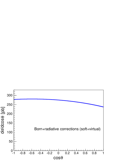
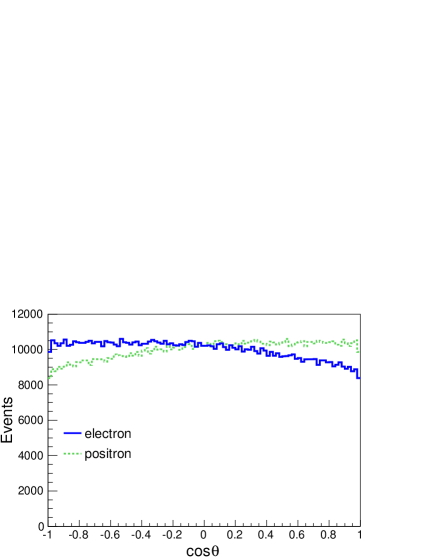
Figure 8: Differential cross section as a function of $\cos\theta$ (top) for a sample of $10^{6}$ generated events (top) for the process $\bar{p}p\to e^{+}e^{-}$ including first order virtual and soft-real photon emissions, for $s$= 5.08 GeV², with $|G_{E}|=0.16$ and $|G_{M}|=0.12$. The soft photon threshold is set to $\Delta E/E=1\%$. Bottom: corresponding number of events: the blue solid line (green dashed line) describes the electron (positron) $\cos\theta$ distributions.

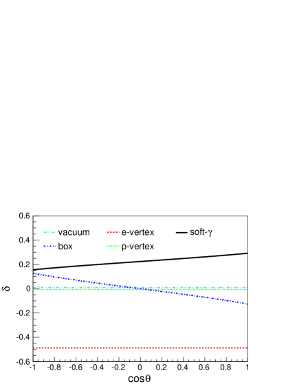
Figure 9: First order radiative corrections: soft photon emission (black solid line), virtual emission at electron vertex (red dashed line), virtual emission at the proton vertex (green dotted line), box diagrams (blue dashed-dotted line), vacuum polarization (Cyan dashed-dotted-dotted line), as a function of the electron c.m.s. production angle, for $s$= 5.08 GeV² and $\Delta E/E=1\%.$

The formulas without approximations from Ref.  [29], have been implemented, except for Eq. (27) of  [29]. The soft $ep$ interference has been calculated from Ref. [33]. The difference between the exact first order calculation and the approximated one for the soft $ep$ interference are mostly due to the approximation $s\sim-t\sim-u\gg M^{2}$ in Eq.(27) of Ref. [29], which does not hold in the backward and forward angular regions. The results are reported in Fig. 10 for $\omega/E=1\%$ at $s$=5.08 GeV² (top) and $s$=12.9 GeV² (bottom). These figures illustrate the effect of neglecting the proton mass and of accounting for the central angular region only.

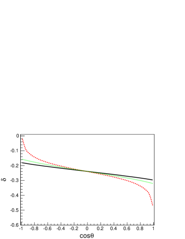
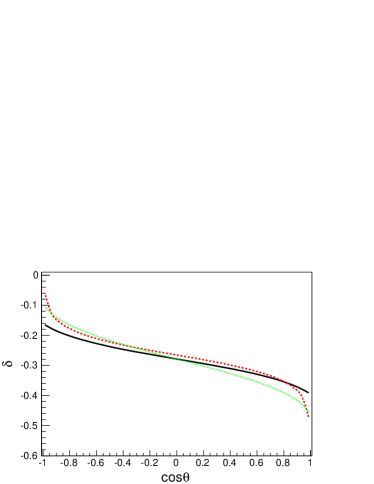
Figure 10: Soft real and virtual radiative corrections for $\omega/E=1\%$ at $s$=5.08 GeV² (top) and $s$=12.9 GeV² (bottom). Calculations are - from [29] (red dashed line) - replacing the soft $ep$ interference from [31] (green dotted line) - and from [33] (black solid line).

4.2 Virtual, soft and hard real photon emission

Table 3: The $\lambda$-independence of total relative corrections to cross section including hard photon emission at different scattering angles $\theta$ and maximum Bremsstrahlung photon energies $\omega_{\rm max}$. $V$ stands for virtual corrections (extracted from (32)), $R$ is for real photon emission contribution according to (64).

$\theta$	$\lambda/\sqrt{s}$	$\omega_{\rm max}=0.1\sqrt{s}/2$			$\omega_{\rm max}=0.3\sqrt{s}/2$
(deg)		$V$	$R$	$V+R$	$V$	$R$	$V+R$
30	$10^{-8}$	-0.83064	0.76575	-0.06490	-0.83064	0.82476	-0.00589
	$10^{-7}$	-0.67912	0.61423	-0.06489	-0.67912	0.67323	-0.00588
	$10^{-6}$	-0.52759	0.46274	-0.06485	-0.52759	0.52177	-0.00582
	$10^{-5}$	-0.37606	0.31166	-0.06440	-0.37606	0.37066	-0.00540
	$10^{-4}$	-0.22454	0.16885	-0.05568	-0.22454	0.22329	-0.00125
	$10^{-3}$	-0.07301	0.06534	-0.00767	-0.07301	0.10193	0.02892
90	$10^{-8}$	-1.00443	0.91202	-0.09241	-1.00443	0.98130	-0.02313
	$10^{-7}$	-0.83053	0.73813	-0.09240	-0.83053	0.80742	-0.02312
	$10^{-6}$	-0.65664	0.56429	-0.09235	-0.65664	0.63357	-0.02307
	$10^{-5}$	-0.48275	0.39084	-0.09192	-0.48275	0.46010	-0.02265
	$10^{-4}$	-0.30886	0.22565	-0.08321	-0.30886	0.29027	-0.01859
	$10^{-3}$	-0.13497	0.09976	-0.03521	-0.13497	0.14634	0.01137
150	$10^{-8}$	-1.17770	1.05818	-0.11952	-1.17770	1.13727	-0.04043
	$10^{-7}$	-0.98144	0.86192	-0.11952	-0.98144	0.94102	-0.04042
	$10^{-6}$	-0.78518	0.66571	-0.11948	-0.78518	0.74480	-0.04039
	$10^{-5}$	-0.58893	0.46987	-0.11906	-0.58893	0.54895	-0.03998
	$10^{-4}$	-0.39267	0.28229	-0.11038	-0.39267	0.35665	-0.03602
	$10^{-3}$	-0.19641	0.13402	-0.06239	-0.19641	0.19014	-0.00627

Next we prove the $\lambda$-dependence cancellation when including hard photon emission. In Table 3 the virtual corrections and the sum of soft and hard photon emission (using Eq. (64) are shown. The stability of the sum with respect to $\lambda$ is worse than in Table 2, due to the Monte Carlo multidimensional integration of hard photon emission. Howevere, the stability of the numerical results including hard photon remains at the $1\%$ level or better.

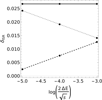
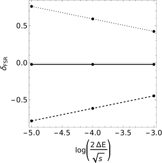
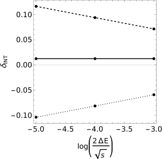
Figure 11: Illustration of the cancellation of the soft photon parameter $\Delta E$ in the sum of soft and hard photon emission at $s=5.08\leavevmode\nobreak\ \mbox{GeV}^{2}$. The dashed line is the sum of virtual corrections with emission of soft photons with energy below $\Delta E$. The dotted line is the hard photon emission with energy larger then $\Delta E$. The solid line is the sum of these two contributions. From top to bottom: ISR, FSR and INT corrections.

Finally we show that the total radiative corrections including virtual, soft and hard photon emission do not depend on the soft photon parameter $\Delta E$ which delimits the regions of soft and hard photon emission. In Fig. 11 the three components charge-even : ISR, FSR and their charge-odd interference of the radiative corrections at $s$ = 5.08 GeV² are illustrated, from top to bottom. The dashed lines are the sum of virtual corrections with the corresponding soft photon emission with photon energy $\omega<\Delta E$. The boson self energy contributions are included in the upper plot. The dotted lines correspond to hard photon emission with photon energy $\omega>\Delta E$. SThe solid lines are the sum of these two contributions. One can see that when scanning over a wide range for $\Delta E$, the soft and hard photon emissions show a $\Delta E$-dependence while their sum does not.

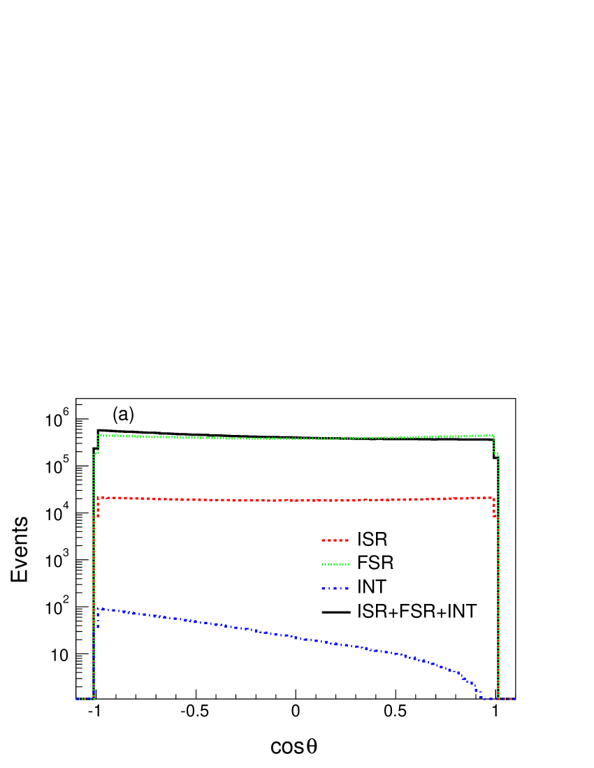
(a)

(b)

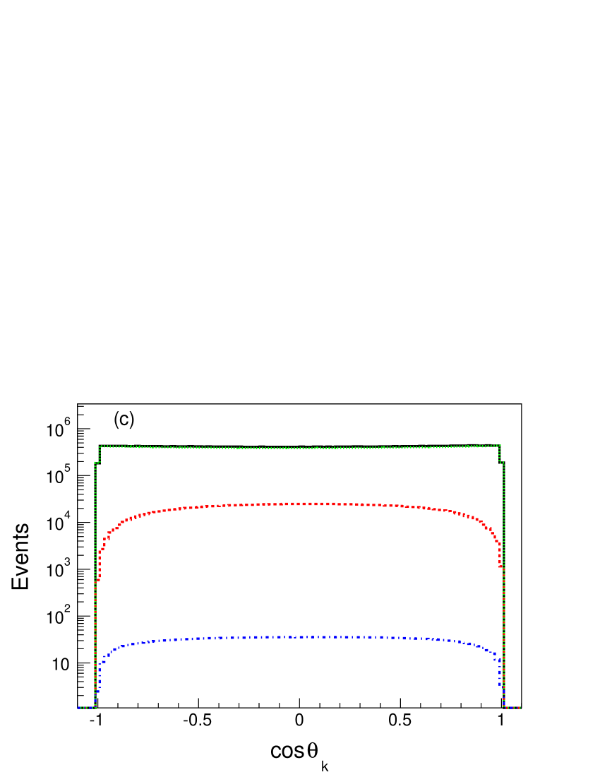
(c)

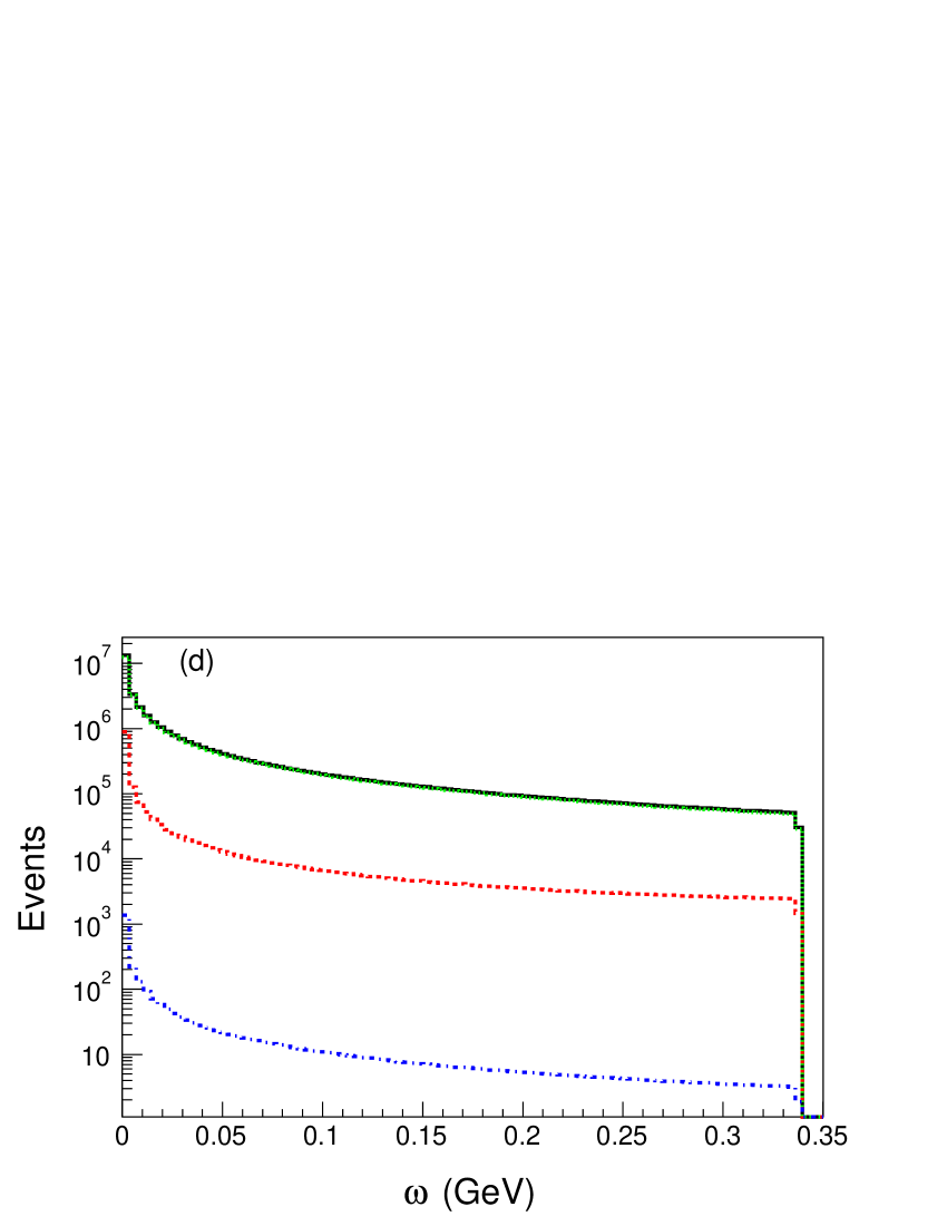
(d)

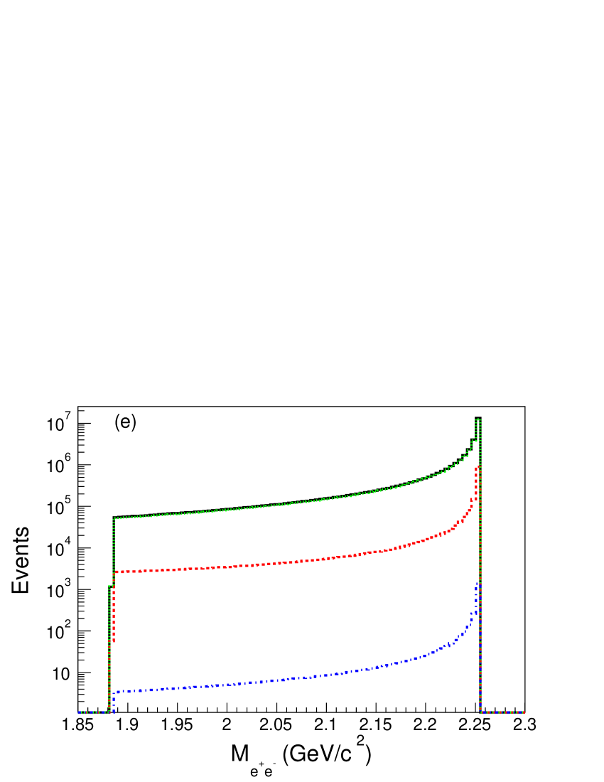
(e)

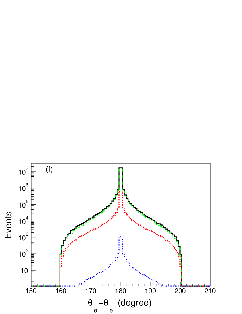
(f)

Figure 12: Dependence of the five-fold Bremsstrahlung cross section (formula (64)) in the c.m.s, as output of the Monte Carlo event generator, on: (a) the electron angle $\cos\theta$, (b) the opening angle between the electron and the photon $\cos\theta_{(e^{-},\gamma)}$, (c) the photon angle $\cos\theta_{k}$, (d) the photon energy $\omega$, (e) the electron-positron invariant mass $M_{e^{+}e^{-}}$, and (f) the sum of polar angles of the electron and positron. The red dotted histograms, the green dashed histograms, the dashed-dotted blue histograms and the black solid histograms describe the generated events from ISR, FSR, INT and ISR+FSR+INT, respectively. The c.m energy squared is $s=5.08$ GeV² ($p_{lab}=1.5$ GeV/c), the energy of the emitted photon is between $\lambda=10^{-5}\sqrt{s}/2$ and $w_{max}=0.3\sqrt{s}/2$. The number of generated events is $10^{7}$. The distributions are normalized to the numbers of the expected events according to their cross sections and a luminosity of 2 fb^-2.

Figure 12 shows one-dimensional distributions of the Bremsstrahlung cross section (formula (64)) in the c.m.s at $s=$5.08 GeV². The histograms are the outputs of the Monte Carlo event generator for the events corresponding to ISR (red dotted histograms) , FSR (green dashed histograms) and INT (dashed-dotted blue histograms). The total contributions from ISR+FSR+INT events are plotted as black solid lines.

The distributions of the electron polar angle $\cos\theta$ are illustrated in Fig. 12a. One can see that the interference between photons emitted from initial and final states leads to a forward-backward asymmetry in $\cos\theta$ distribution. The differential cross section of the reaction $\bar{p}\to e^{+}e^{-}\gamma$ reaches its highest values at small photon polar angles relative to the direction of the final state electron and positron (Fig. 12b). The distributions of the photon polar angle $\cos\theta_{k}$ are illustrated in Fig. 12c. In the considered reference system, this angle is the opening angle between the photon and this initial state antiproton. Fig. 12d shows the energy distributions of the emitted photon. Soft and hard photon contributions are included.

In these simulations, the photon energy range is taken from $\lambda=10^{-5}\sqrt{s}$ up to $w_{max}=0.3\sqrt{s}/2$. The value of $w_{max}$ is typically above the energy resolution of the PANDA detector and can be used as an experimental cut to select the signal events $p\bar{p}\to e^{+}e^{-}(\gamma)$ (e.g $\omega<w_{max}$. To suppress the background channels, one can also apply a cut on the invariant mass $M_{e^{+}e^{-}}$ of the $e^{+}e^{-}$ system (Fig. 12e), e.g. $a<M_{e^{+}e^{-}}<b$, where the values of $a$ and $b$ are chosen in order to achieve a high background suppression factor keeping a good signal efficiency [25].

The $M_{e^{+}e^{-}}$ for the Born events ($p\bar{p}\to e^{+}e^{-}$) corresponds to a c.m. s. energy $\sqrt{s}=2.25$ GeV. The radiative tail is due to hard photon emission. Another relevant kinematic variable for the signal selection is the sum of the electron and positron polar angles ($\theta_{e^{+}}+\theta$). The electron and positron are emitted back to back in the c.m.s (($\theta_{e^{+}}+\theta$)=180^∘). The tails shown around $180^{\circ}$ (Fig. 12f) are due to hard photon emission.

The differential cross section for the process $\bar{p}\to e^{+}e^{-}\gamma$ presents some peaks that correspond to the situation when the emitted photon is collinear to the direction of the electron or positron. This leads to a reduction in the efficiency and in the accuracy of the Monte Carlo algorithm. To absorb these peaks and allow a fast event generation, the Importance Sampling method [38] has been used. Jacobian transformations of the two variables, the photon polar angle and energy, have been performed as described in Ref. [39].

5 Conclusion

The precise measurements of the TL electromagnetic FFs of the proton expected at the future PANDA experiment via the reaction $\bar{p}p\rightarrow e^{+}e^{-}$, require to take into account radiative corrections. Although several packages dealing with radiative corrections are available on the market, none of them is entirely suitable for PANDA. In this work, the next-to-leading-order (NLO) $\bar{p}p\rightarrow e^{+}e^{-}$ differential cross section has been calculated in the point-like approximation, including both virtual and real corrections.

Relying on the method developed in Ref. [29], the full set of calculated virtual corrections include vacuum polarisztion (with all leptons and a point-like pion in the photon loop), corrections to both electron and proton vertex, and two photon exchange. On the other hand, real corrections including initial and final state radiation, and the interference between them, have been re-calculated in this work, in the spirit of the classic references [32] and [33] for the reactions $e^{+}e^{-}\rightarrow\mu^{+}\mu^{-}$. In the soft photon regime, infrared divergences from singular virtual diagrams are cancelled out with the corresponding real diagrams. On the other hand, the regularisation of infrared divergencies of the Bremsstrahlung cross section is based on the introduaction of a small photon mass as a parameter, which makes the calculation applicable to both the soft and hard photon regimes. The calculated cross section is at the basis of two computer codes which can be included in the PANDA physics analysis framework.

6 Acknowledgments

The authors thank H. Czyz for interest in this work and useful suggestions. Three of us (Yu.M. B., V.A. Z., and E. T.-G.) thank the Helmholtz Institute Mainz for warm hospitality and support. This work was supported by the German Ministry for Education and Research (BMBF) under grant number 05P12UMFP9 and under grant number 05P19UMFP1.

Appendix A Kinematical quantities in c.m.s expressed in terms of invariants

The expression of the physical kinematical variables are given in terms of the radiative invariants (see Table 1). All formulas in this section are given neglecting the quantities $m$ and $\lambda$.

1. The photon energy:

   $$\omega=\frac{z+v}{2\sqrt{s}}.$$ (65)

2. The photon momentum ${\bf k}$ polar angle:

   $$\cos\theta_{k}=\frac{z_{1}-v_{1}}{2\omega\sqrt{s-4M^{2}}}.$$ (66)

3. The photon momentum ${\bf k}$ azimuthal angle:

   $$\cos\varphi_{k}=-\frac{A+\cos\theta\cos\theta_{k}}{\sin\theta\sin\theta_{k}},$$ (67)

   where

   $$A=\frac{v-z-2\omega\left(2\varepsilon_{2}-\sqrt{s}\right)}{4\omega\sqrt{\varepsilon_{2}^{2}-m^{2}}}.$$ (68)

4. The electron energy:

   $$\varepsilon_{2}=\begin{cases}\left(1-\frac{z}{s}\right)\frac{\sqrt{s}}{2},\qquad\qquad\mbox{if}\ v>z\frac{s-z}{s+z},\\ \left(1-\frac{v}{s-z-v}\right)\frac{\sqrt{s}}{2},\qquad\!\!\mbox{if}\ v<z\frac{s-z}{s+z}.\end{cases}$$ (69)

5. The positron energy:

   $$\varepsilon_{1}=\sqrt{s}-\varepsilon_{2}-\omega.$$ (70)

References

- [1] A. Zichichi, S.M. Berman, N. Cabibbo, and Raoul Gatto. Proton anti-proton annihilation into electrons, muons and vector bosons. Nuovo Cim., 24:170–180, 1962.
- [2] Simone Pacetti, Rinaldo Baldini Ferroli, and Egle Tomasi-Gustafsson. Proton electromagnetic form factors: Basic notions, present achievements and future perspectives. Phys. Rep., 550-551:1–103, 2015.
- [3] Klaus Peters, Lars Schmitt, Tobias Stockmanns, and Johan Messchendorp. PANDA: Strong Interaction Studies with Antiprotons. Nucl. Phys. News, 27(3):24–28, 2017.
- [4] Peter Spiller et al. Status of the FAIR Project. In Proceedings, 9th International Particle Accelerator Conference (IPAC 2018): Vancouver, BC Canada, page MOZGBF2, 2018.
- [5] A.I. Akhiezer and Mikhail.P. Rekalo. Polarization phenomena in electron scattering by protons in the high energy region. Sov. Phys. Dokl., 13:572, 1968. [Dokl. Akad. Nauk Ser. Fiz. 180, 1081 (1968)].
- [6] A.I. Akhiezer and Mikhail.P. Rekalo. Polarization effects in the scattering of leptons by hadrons. Sov. J. Part.Nucl., 4:277, 1974. [Fiz. Elem. Chast. Atom. Yadra 4, 662 (1973)].
- [7] A. J. R. Puckett et al. Polarization Transfer Observables in Elastic Electron Proton Scattering at 2.5, 5.2, 6.8, and 8.5 GeV2. Phys. Rev., C96(5):055203, 2017.
- [8] M.N. Rosenbluth. High Energy Elastic Scattering of Electrons on Protons. Phys.Rev., 79:615–619, 1950.
- [9] Simone Pacetti and Egle Tomasi-Gustafsson. Form factor ratio from unpolarized elastic electron-proton scattering. Phys. Rev., C94(5):055202, 2016.
- [10] Egle Tomasi-Gustafsson. On radiative corrections for unpolarized electron proton elastic scattering. Phys. Part. Nucl. Lett., 4:281–288, 2007.
- [11] Yu. M. Bystritskiy, E. A. Kuraev, and E. Tomasi-Gustafsson. Structure function method applied to polarized and unpolarized electron-proton scattering: A solution of the GE(p)/GM(p) discrepancy. Phys. Rev., C75:015207, 2007.
- [12] A. V. Gramolin and D. M. Nikolenko. Reanalysis of Rosenbluth measurements of the proton form factors. Phys. Rev., C93(5):055201, 2016.
- [13] A. Afanasev, P. G. Blunden, D. Hasell, and B. A. Raue. Two-photon exchange in elastic electron–proton scattering. Prog. Part. Nucl. Phys., 95:245–278, 2017.
- [14] P. G. Blunden and W. Melnitchouk. Dispersive approach to two-photon exchange in elastic electron-proton scattering. Phys. Rev., C95(6):065209, 2017.
- [15] J. Guttmann, N. Kivel, M. Meziane, and M. Vanderhaeghen. Determination of two-photon exchange amplitudes from elastic electron-proton scattering data. Eur. Phys. J., A47:77, 2011.
- [16] V. V. Bytev and E. Tomasi-Gustafsson. Updated analysis of recent results on electron and positron elastic scattering on the proton. Phys. Rev., C99(2):025205, 2019.
- [17] M.P. Rekalo and E. Tomasi-Gustafsson. Complete experiment in scattering in presence of two-photon exchange. Nucl.Phys., A740:271–286, 2004.
- [18] M.P. Rekalo and E. Tomasi-Gustafsson. Polarization phenomena in elastic e-+ N scattering, for axial parametrization of two photon exchange. Nucl.Phys., A742:322–334, 2004.
- [19] G.I. Gakh and E. Tomasi-Gustafsson. Polarization effects in the reaction in presence of two-photon exchange. Nucl.Phys., A761:120–131, 2005.
- [20] G.I. Gakh and E. Tomasi-Gustafsson. General analysis of polarization phenomena in for axial parametrization of two-photon exchange. Nucl.Phys., A771:169–183, 2006.
- [21] Henryk Czyz, Johann H. Kuhn, Elzbieta Nowak, and German Rodrigo. Nucleon form-factors, B meson factories and the radiative return. Eur. Phys. J., C35:527–536, 2004.
- [22] Henryk Czyz, Johann H. Kühn, and Szymon Tracz. Nucleon form factors and final state radiative corrections to . Phys. Rev., D90(11):114021, 2014.
- [23] E. A. Kuraev and Victor S. Fadin. On Radiative Corrections to Single Photon Annihilation at High-Energy. Sov. J. Nucl. Phys., 41:466–472, 1985. [Yad. Fiz.41,733(1985)].
- [24] M. Sudol et al. Feasibility studies of the time-like proton electromagnetic form factor measurements with PANDA at FAIR. Eur. Phys. J., A44:373–384, 2010.
- [25] B. Singh et al. Feasibility studies of time-like proton electromagnetic form factors at ANDA at FAIR. Eur. Phys. J., A52(10):325, 2016.
- [26] P. Golonka and Z. Was. Next to Leading Logarithms and the PHOTOS Monte Carlo. Eur. Phys. J., C50:53–62, 2007.
- [27] R. G. Sachs. High-energy behavior of nucleon electromagnetic form factors. Phys. Rev., 126:2256–2260, Jun 1962.
- [28] F. Iachello and Q. Wan. Structure of the nucleon from electromagnetic timelike form factors. Phys.Rev., C69:055204, 2004.
- [29] A.I. Ahmadov, V.V. Bytev, E.A. Kuraev, and E. Tomasi-Gustafsson. Radiative proton-antiproton annihilation to a lepton pair. Phys. Rev., D82:094016, 2010.
- [30] F. Bloch and A. Nordsieck. Note on the Radiation Field of the electron. Phys. Rev., 52:54–59, 1937.
- [31] Jacques Van de Wiele and Saro Ong. Radiative corrections in nucleon time-like form factors measurements. Eur. Phys. J., A49:18, 2013.
- [32] Frits A. Berends, K. J. F. Gaemer, and R. Gastmans. Hard photon corrections for the process . Nucl. Phys., B57:381–400, 1973. [Erratum: Nucl. Phys. B75, 546 (1974)].
- [33] Frits A. Berends, K. J. F. Gaemers, and R. Gastmans. Contribution to the angular asymmetry in . Nucl. Phys., B63:381–397, 1973.
- [34] E. A. Kuraev and G. V. Meledin. QED Distributions for Hard Photon Emission in . Nucl. Phys., B122:485–492, 1977.
- [35] A. G. Aleksejevs, S. G. Barkanova, and V. A. Zykunov. Method for Taking into Account Hard-Photon Emission in Four-Fermion Processes. Phys. Atom. Nucl., 79(1):78–94, 2016. [Yad. Fiz. 79, 20 (2016)].
- [36] E. Byckling and K. Kajantie. Particle Kinematics. John Wiley and Sons, London New York Sydney Toronto, 1973.
- [37] V. A. Zykunov. New method for taking into account radiative events in the MOLLER inclusive experiment. Phys. Atom. Nucl., 80(4):699–706, 2017. [Yad. Fiz. 80, 388 (2017)].
- [38] J. M. Hammersley and D. C. Handscomb. Monte carlo methods (methuen. london, 1964): F. james. rep. prog. phys. 43 (1980) 1145.
- [39] Michele Caffo and H. Czyz. BHAGEN-1PH: A Monte Carlo event generator for radiative Bhabha scattering. Comput. Phys. Commun., 100:99–118, 1997.