Entanglement conductance as a characterization of delocalized-localized phase transition in free fermion models

Abstract

We study entanglement Hamiltonian (EH) associated with the reduced density matrix of free fermion models in delocalized-localized Anderson phase transition. We show numerically that the structure of the EH matrix differentiates the delocalized from the localized phase. In the delocalized phase, EH becomes a long-range Hamiltonian but is short-range in the localized phase, no matter what the configuration of the system’s Hamiltonian is (whether it is long or short range). With this view, we introduce the entanglement conductance (EC), which quantifies how much EH is long-range and propose it as an alternative quantity to measure entanglement in the Anderson phase transition, by which we locate the phase transition point of some one-dimensional free fermion models; and also by applying the finite size method to the EC, we find three-dimensional Anderson phase transition critical disorder strength.

I Introduction

Entanglement is a purely quantum concept: two particles that have interacted in the past, never can be considered as two independent particlesEinstein et al. (1935); Schrödinger (1935), rather they have to be described as a unified entity. This concept is used in the quantum information science as a physics resource with the applications in quantum communicationDuan et al. (2001); Briegel et al. (1998), cryptographyEkert (1991); Gisin et al. (2002); Bennett (1992), teleportationBraunstein and Kimble (1998); Bouwmeester et al. (1997), and computer sciences Nielsen and Chuang (2002); Kane (1998); Shor (1995). Later, condensed matter physicists found this concept useful to characterize different phases, since entanglement indirectly measures the amount of correlation in the system. To quantify entanglement in a system, people have used different measures. Entanglement Entropy (EE) is the most famous candidate in a pure ground sate of a system; although there are other alternative measures available for the ground state, and for excited stateHorodecki et al. (2009) where the system is in a mixed state. People in addition developed methods to measure entanglement in experiment.Sackett et al. (2000); Raimond et al. (2001); Cornfeld et al. (2018)

Among many other applications, EE can be specially beneficial for a delocalized-localized phase transition, where state of the system changes as disorder in the system is varied. In the delocalized phase, the correlation in the system is larger than in the localized phase and thus we see larger EE.Le Hur et al. (2007) Delocalized-localized phase transition is manifested in lattice systems by Anderson modelAnderson (1958) which is a tight binding model with constant tunneling amplitude and random on-site energies. With uncorrelated disorderEvers and Mirlin (2008), we know that the system is localized with any infinitesimal amount of disorder in one and two dimensions, and thus there is no Anderson phase transition. While in three dimensions $3D$, at a critical disorder, scattering of fermions by impurities becomes completely destructive and state of the system becomes localized.Markoš (2006) However, with correlated disorder, systems in $1D$ and $2D$ can also exhibit Anderson phase transitionEvers and Mirlin (2008), some of which are used in this paper to verify our idea.

Anderson phase transition happens at zero temperature where fluctuations has quantum nature only. It is among the class of second order phase transition, where observables of the system at the phase transition point become length-scale independent and by finite size scaling one finds the phase transition point and the corresponding universal critical exponents.Slevin and Ohtsuki (2014)

Aside from the EE, it is also found the entanglement spectrumLi and Haldane (2008); Cho et al. (2017); Predin (2017); Pollmann et al. (2010); Calabrese and Lefevre (2008); Qi et al. (2012) and also the eigenmodes of the entanglement HamiltonianPouranvari and Yang (2014, 2013, 2015) are useful to characterize different phases. What is left, is to look at the entanglement Hamiltonian (EH) matrix to see what information about the system we can catch. EH of a subsystem has been studied from another perspectives. In a studyEisler and Peschel (2017), the explicit expression for the EH matrix elements in the ground state of free fermion models has been reported. In another studyZhu et al. (2019), operator form of the EH is constructed based on one entangled mode of the reduced density matrix. People also found that at the extreme limit of strong coupling between two chosen subsystems, EH of a subsystem and its Hamiltonian are proportional. Peschel and Chung (2011); Moradi and Abouie (2016) On the other hand, for a non-zero temperature, in a highly excited state, reduced density of a subsystem becomes the thermal density and correspondingly, EH of subsystem relates to the subsystem’s Hamiltonian.Garrison and Grover (2018) In this paper, we emphasize on the fact that structure of the ground state EH of a chosen subsystem possesses physical information and thus useful to distinguish different phases of the system. More specifically, we show that, subsystem EH made by ground state of the whole system in a free fermion model, has distinguishable configurations in delocalized and localized phases of Anderson phase transition: EH is long-range in delocalized phase and short-range in localized phase. In addition, to quantify EH configuration, we use the notion of conductance of entanglement Hamiltonian. By using EH conductance as an indicator, we distinguish localized and delocalized phases, and also we locate exactly the Anderson phase transition point.

This paper is structured as follows: in Section II the $1D$ models and the $3D$ Anderson model that we use in this paper are explained; we also shortly explain how to obtain the EH for the ground state. In Section III, EH structures in both delocalized and localized phases are studied and contrasted. Then we introduce EH conductance in section IV as an indicator of delocalized and localized phases. The conclusion and some suggestions for future works are presented in section V.

II Models and Method

We consider $1D$ free fermion models and also the $3D$ Anderson model. In the following, we introduce these models and review their delocalized-localized phase transitions that has been proved analytically and numerically before.

The first model we consider, is the generalized Aubry-Andre (gAA) model. It is a $1D$ tight binding model with constant nearest-neighbor hopping amplitude $t$:

$$\mathcal{H}=\sum_{<ij>}t(c_{i}^{\dagger}c_{j}+c_{j}^{\dagger}c_{i})+\sum_{i}\phi_{i}c_{i}^{\dagger}c_{i}$$ (1)

where $<ij>$ stands for nearest-neighbor hopping and the on-site energies $\phi_{i}$ have an incommensurate periodicity with respect to lattice constant (set to $1$ here):

$$\phi_{i}=2\lambda\frac{\cos{(2\pi ib)}}{1-\alpha\cos{(2\pi ib)}},$$ (2)

which $b=\frac{1+\sqrt{5}}{2}$ is the golden ratio (we set $t=-1$ in our calculations). This model is neither completely periodic nor completely random and as illustrated in Ref. [Ganeshan et al., 2015], it has the separating mobility edges of localized and delocalized states at the energy:

$$E_{\text{mobility edge}}=2sgn(\lambda)\frac{|t|-|\lambda|}{\alpha}.$$ (3)

Note that this model has no randomness and delocalized phase happens by the incommensurate periodicity of on-site energy. The special case of Eq. (2) with $\alpha=0$ is the Aubry-Andre (AA) modelAubry and André (1980) with delocalized ($\lambda<1$) and localized ($\lambda>1$) phases. AA model has no mobility edges, i.e. all states become localized in the localized phase.

Another model is the power-law random banded matrix model (PRBM)Mirlin et al. (1996) that is a long-range hopping model with the following Hamiltonian:

$$\mathcal{H}=\sum_{ij}h_{ij}c_{i}^{\dagger}c_{j},$$ (4)

in which matrix elements $h_{ij}$ are randomly Gaussian distributed numbers, with zero mean and the following variance (if we use the periodic boundary condition):

$$\left<|h_{ij}|^{2}\right>=\left[{1+\left(\frac{\sin{\pi(i-j)/N}}{b\pi/N}\right)^{2\alpha}}\right]^{-1},$$ (5)

where $N$ is the system size and we set $b=1$. In the limiting case of $\alpha\gg 1$, the variance $\left<|h_{ij}|^{2}\right>$ approaches zero for the next nearest neighbor couplings and further, and thus the Hamiltonian of the system will be a Hamiltonian with short-range couplings. On the other hand, when $\alpha\ll 1$, $\left<|h_{ij}|^{2}\right>$ approaches to $1/2$ for all couplings, thus yield to a long-range Hamiltonian with all couplings to be non-zero. Therefore, the system goes through Anderson phase transition at $\alpha=1$, it is in delocalized phase for $\alpha<1$ and localized for $\alpha>1$.Mirlin et al. (1996) This model is distinguished and important since different models can be simulated by modifying the $b$ parameter.José and Cordery (1986); Balatsky and Salkola (1996); Altshuler and Levitov (1997); Ponomarev and Silvestrov (1997)

One another model we consider is the power-law random bond disordered Anderson model (PRBA)Lima et al. (2004) which is a $1D$ model with the Hamiltonian of Eq. (4), where on-site energies are zero, and long-range hopping amplitudes are

$$h_{ij}=\frac{w_{ij}}{|i-j|^{\alpha}},$$ (6)

where $w_{i,j}$’s are uniformly random numbers distributed between $-1$ and $1$. When $\alpha\ll 1$, hopping amplitude becomes slow decaying, and the Hamiltonian is long-range. On the other hand, for $\alpha\gg 1$, hopping amplitude goes very fast to zero and we have a short-range Hamiltonian. Therefore, there is a phase transition at $\alpha=1$ between delocalized state ($\alpha<1$ with long-range hopping amplitudes) and localized state ($\alpha>1$, with short-range hopping amplitudes).

Finally, we also consider the three dimensional Anderson model (the $3D$ version of Eq. (1)) with constant nearest-neighbor hopping amplitudes, $t=-1$, and randomly distributed on-site energies. We use Gaussian distribution with mean zero and variance $W$ where the Anderson phase transition happens at $W\approx 6$Slevin and Ohtsuki (2014), the system is in delocalized phase for $W<6$ and localized for $W>6$.

We note that in gAA and Anderson $3D$ models, the structure of the Hamiltonian matrix is the same in delocalized and localized phases (it is always a short-range Hamiltonian: only the nearest neighbor hopping amplitude is non-zero). However, in the PRBM and PRBA models, the structure of the Hamiltonian matrix is different in the delocalized and localized phases: in the localized phase it is a short-range and in the delocalized phase it is a long-range.

II.1 Entanglement Hamiltonian (EH) for free fermion models

Next, we explain the procedure to obtain Entanglement Hamiltonian for free fermion models. One usually divides the system into two parts in real space, subsystem $A$ form site $1$ to $N_{A}$ and the rest of the system as subsystem $B$. Other type of partition has also been used.Mondragon-Shem et al. (2013); Mondragon-Shem and Hughes (2014); Legner and Neupert (2013) Then, EE is obtained by calculating the von Neumann entropy of the reduced density matrix (RDM) of a chosen subsystem. That is EE = $-tr\rho_{A}\log\rho_{A}$, where $\rho_{A}$ is the RDM of subsystem $A$ computing by tracing over degrees of freedom of subsystem $B$. Since the RDM is a positive definite operator, we can write it as:

$$\rho_{A}=e^{-\mathcal{H}^{ent}},$$ (7)

where $\mathcal{H}^{ent}$ is called entanglement Hamiltonian (EH). For free fermion models (that we consider in this paper) EH is a free fermion Hamiltonian:

$$\mathcal{H}^{ent}=\sum_{ij}^{N_{A}}H^{ent}_{ij}c_{i}^{\dagger}c_{j}.$$ (8)

To obtain the EH numerically in the free fermion models, one first calculates the correlation matrix for the chosen subsystem:

$$C^{A}_{ij}=\langle c_{i}^{\dagger}c_{j}\rangle,\quad i,j=1,\cdots,N_{A}.$$ (9)

In free fermion models that we consider in this paper, we can calculate the correlation matrix based on the eigenvectors of the Hamiltonian, $V$:

$$C^{A}_{ij}=\sum_{k=1}^{N_{\rm F}}V_{ik}V^{\dagger}_{kj},$$ (10)

where $N_{\rm F}$ is the number of fermions. By setting the Fermi energy $E_{\rm F}$, we can obtain the number of fermions $N_{\rm F}$: we fill up the energy levels by fermions until we reach the $E_{\rm F}$. In this paper we set $E_{\rm F}=0$ and for each model and sample we calculate numerically the number of fermions (only for gAA model we change Fermi energy from its lowest value to its highest value and then obtain the number of fermions accordingly).

Correlation matrix is related to $H^{ent}$ asPeschel (2003); Cheong and Henley (2004):

$$H^{ent}=\ln\frac{1-C^{A}}{C^{A}}.$$ (11)

Diagonalizing the correlation matrix and finding its eigenvalues and eigenvectors, we obtain the EH matrix.

III Entanglement Hamiltonian in delocalized-localized phases

In the following we give a picture of the matrix elements of the EH in localized and delocalized phases. Matrix elements of the EH based on Eq. (11) are:

$$H_{ij}^{ent}=\sum_{\ell=1}^{N_{A}}U_{i\ell}\ln\frac{1-\zeta_{\ell}}{\zeta_{\ell}}U^{\ast}_{j\ell},$$ (12)

in which $\{\zeta_{\ell}\}$ and $U$ are the eigenvalues, and the unitary matrix to diagonalize the correlation matrix, respectively.

One special eigenvector of the $U$ matrix, which corresponds to the $\zeta$ closes to $1/2$, has proven to be localized (extended) in the localized (delocalized) phase.Pouranvari and Yang (2014, 2013); Roy and Sharma (2018); Pouranvari (2018) Here, we show that all eigenvectors of EH has this property. To verify it numerically, we plot the $U$ matrix composed of the EH eigenvectors for the PRBM model in Fig. 1; each normalized eigenvector of EH (which is a column in the $U$ matrix) is extended in the delocalized phase and it has only a few non-zero values in the localized phase. Same results obtained for other models we considered in this paper (not shown). Thus, for each eigenvector, a localization length can be defined over which the eigenvector is extended and outside of which it vanishes.

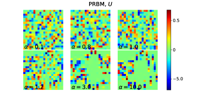
Figure 1: The eigenvectors of EH, i.e. $U$ matrix elements plotted for PRBM model with $N=40$ sites and $N_{A}=20$, as we increase $\alpha$ and go from delocalized phase ($\alpha<1$) to localized phase ($\alpha>1$). Each column is a normalized eigenvector of EH. Deep in the delocalized phase, it is completely extended over all sites, and it becomes localized only over a few sites in localized phase. Plots from top-left to bottom-right correspond to $\alpha=0.1$, 0.8, 1.0, 1.2, 3.0, and 10.0, respectively.

Now, having in mind this localization properties of $U$, we can analyze the EH matrix elements. To obtain $H^{ent}_{i,j}$, as we go from diagonal elements outward, i.e. for $H^{ent}_{i,i+n}$ elements, as we increase $n$, we multiply $U_{i\ell}$ and $U_{i+n,\ell}$ when we sum over $\ell$ in Eq. (12). For the $\ell$th eigenvector, if both $i$ and $i+n$ elements are inside the localization length, we will have a non-zero result; but as soon as one of these elements falls outside of localization length, we will have a vanishing result. In the localized phase where columns of $U$ matrix become localized, then we get faster vanishing results for $H^{ent}_{ij}$ as we go off-digonal. On the other hand, in the delocalized phase with extended EH eigenvectors, localization length increases and we have more non-zero elements for $H^{ent}_{ij}$. Therefore, in the localized phase we expect to have a short-range hopping matrix for the EH with only a few non-zero off-diagonal elements, while in the extended phase the EH becomes long-range. EH of AA, PRBM and Anderson $3D$ models are plotted in Figs. 2, 3, and 4, respectively, in delocalized and localized phases. As we can see, the EH is a long-range Hamiltonian (with many non-zero off-diagonal elements) in the delocalized phase, and as we approach to the localized phase, it becomes short-range. In the extreme situation, deep in the localized phase, diagonal elements become much larger and the off diagonal elements become zero; on the other hand, deep in delocalized phase, diagonal elements become zero. Similar results are obtained for PRBA and gAA models (not shown here).

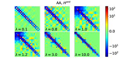
Figure 2: The EH matrix elements plotted for AA model of $N=40$ sites, and $N_{A}=20$, as we increase $\lambda$ and go from delocalized phase ($\lambda<1$) to localized phase ($\lambda>1$). We set Fermi energy $E_{\rm F}=0$.

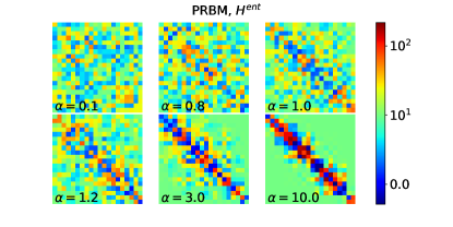
Figure 3: The EH matrix elements of PRBM model with $N=40$ sites and $N_{A}=20$, as we increase $\alpha$ and go from delocalized phase ($\alpha<1$) to localized phase ($\alpha>1$). We set Fermi energy $E_{\rm F}=0$.

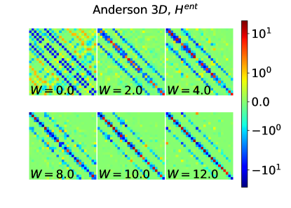
Figure 4: The EH matrix elements plotted for Anderson $3D$ model, with $N=6\times 6\times 6$ and $N_{A}=N/2$, as we increase the disorder strength $W$ and go from delocalized phase ($W<6$) to localized phase ($W>6$). We set Fermi energy $E_{\rm F}=0$. We plot only one quarter of the EH. We note that Anderson $3D$ model has mobility edges at both tail of the spectrum, separating the delocalized and localized phases. Three upper plots correspond to the case when we are in the delocalized phase and three lower case correspond to the localized phase.

This observation is true either for systems with Hamiltonians that are short-range in both localized and delocalized phases (AA, and Anderson models), or for system that its Hamiltonian is short-range in localized and long-range in delocalized phase (PRBM, and PRBA models). Thus, no matter the structure of the Hamiltonian of the system is, the entanglement Hamiltonian is long-range in delocalized phase and short-range in localized phase.

IV Entanglement Conductance (EC)

In the previous section, we showed that by looking at the structure of the EH matrix, different phases can be distinguished; as we go from localized to delocalized phase, EH matrix gains more non-zero amplitudes for far-distances hopping. Although in the pattern of the EH matrix the difference between these phases is obviously seen (at least in the extreme cases deep in localized and delocalized phases), but we need a quantified measure to characterize different phases only by a number and more importantly to identify the delocalized-localized phase transition point. EH (which is a free fermion Hamiltonian) can be considered as a Hamiltonian, describing a system of fermions hopping between arbitrary sites, based on the range of the hopping parameter. When the EH is long-range, fermions can hop between far-distances sites and thus it is expected transportation of these fermions to be easy. On the other hand, if EH is a short-range Hamiltonian, hopping of the fermions would be limited to short-distances sites and transportation becomes harder. In this regard, conductance of a free fermion model described by the EH could be a good candidate to distinguish long-range and short-range Hamiltonians and consequently between delocalized and localized phases. But, EH is not actually the Hamiltonian of a subsystem which we then put it between two contacts and measure it conductance. So, we will encounter conceptual difficulties if we apply the same procedure of calculating conductance to EH. Therefore, we introduce a new quantity, based on the conductanceJavan Mard et al. (2015) in the following way:

$$G = H_{ent}^{-1},$$

$$g_{ent} = G_{1N}G_{N1},$$ (13)

where $H_{ent}^{-1}$ is the inverse of the EH, $G_{1N}$ and $G_{N1}$ are respectively the $(1,N)$ and $(N,1)$ elements of the $G$ matrix. We dub $g_{ent}$ as entanglement conductance. Based on the fact that $G$ is a symmetric matrix, $g_{ent}$ is a positive-definite number. When we have randomness in our employed models, we have to average over samples to obtain the $g_{ent}$. We use geometric averaging, since the obtained numbers ranges over large order of magnitudes. The EC, $g_{ent}$, is plotted for AA, PRBA, and PRBM models in Fig. 5. AA model has a short-range Hamiltonian (in both delocalized and localized phases), on the contrary PRBA and PRBM have a short-range Hamiltonian in localized and a long-range one in delocalized phase. As we can see in Fig. 5, the EC in the delocalized phase is non-zero and it goes to zero very fast in the localized phase, and thus determines the phase transition point exactly. In addition we calculate the EC for gAA model (see Fig. 6.) which has mobility edges between delocalized and localized phases. As we can see $g_{ent}$ sharply determines the mobility edges.

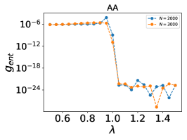
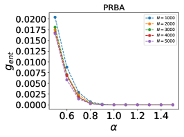
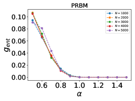
Figure 5: The EC ($g_{ent}$) for the AA model versus $\lambda$ (left), for the PRBA model versus $\alpha$ (middle), and for the PRBM model versus $\alpha$ (right). In three cases $g_{ent}$ goes to zero in the localized phase and it determines the phase transition point, exactly. In AA model we do not have randomness, so one sample is considered. In PRBA, the number of sample systems varies between $10^{5}$ for small $N$ and $10^{3}$ for the largest $N$. In PRBM, the number of sample systems varies between $10^{4}$ for small $N$ and $10^{3}$ for the largest $N$.

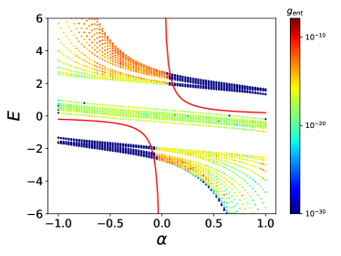
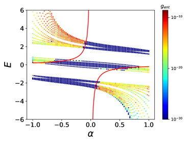
Figure 6: The EC ($g_{ent}$) for gAA model of $N=500$ sites as we change both $\lambda$ and also the number of fermions (or the Fermi energy). In the left panel we set $\lambda=-1.1$ and in the right panel $\lambda=0.9$. Red lines are the mobility edges according to Eq. (3). We can see that $g_{ent}$ sharply determines the mobility edges between delocalized and localized phases.

The EC for the Anderson $3D$ model is also plotted in Fig. 7. For this model $g_{ent}$ does not go to zero sharply in localized phase and thus it does not locate the phase transition point; but by applying finite size scaling to the EC we are able to calculate the critical disorder strength $W_{c}$ and the corresponding critical exponent for localization length, $\nu$. Our numerical calculations yields to $W_{c}=6.1$, which is consistent with numerical results obtained beforeSlevin and Ohtsuki (2014). As it is indicated in Fig. 7, $g_{c}$ changes with system size $N$. So, we re-scale $g_{ent}$ by $g_{c}$. To obtain $W_{c}$ and $\nu$ we plot $g_{ent}/g_{c}$ versus $N/\xi$ (where $\xi$ is a length scale for the EH, similar to the localization length of the Hamiltonian, to show that $g_{ent}/g_{c}$ is scale invariant) for different values of $W$, then we tune $W_{c}$ and $\xi$ to have two branches of curves, one for delocalized and another for localized phase. $\nu$ is given by slope of $1/\xi$ versus $W-W_{c}$ in log-log scale for localized phase.

Figure 7: Left panel: The EC ($g_{ent}$) for the Anderson $3D$ model as we vary $W$ for different system sizes. Middle panel: finite size scaling of EC to find the critical disorder strength. Right panel: behavior of $g_{ent}$ at the critical point versus system size $N$. In the inset plot, $1/\xi$ is plotted versus $W-W_{c}$ in the localized phase to obtain critical exponent $\nu$. The procedure of finding $W_{c}$ is as follows. First we choose a critical $W_{c}$, and plot the entanglement conductance $g_{ent}/g_{c}$ versus $N/\xi$, for different values of $W$. We then tune the parameter $\xi$ until we obtain two branches for EC curve (one for delocalized phase and another for localized phase). While tuning $\xi$, we do our best to have the most smooth curve. Each branch must be appeared as a continuous curve. This procedure is also applied to another choice of $W_{c}$. By comparing the plots of different $W_{c}$, we then conclude which plot is better and we choose the $W_{c}$. Our calculations yield to $W_{c}=6.1$, and $\nu\approx 1.26$. Number of sample systems varies between $20000$ for small $N$ and $2000$ for the largest $N$.

r7ptb66pt

V Conclusion

In this paper, we studied the structure of the entanglement Hamiltonian. We showed that, independent of the Hamiltonian of the system that can be either long-range or short-range, EH is long-range in delocalized phase and short range in localized phase. This is due to the fact that the EH is written in terms of single particle correlation functions. We introduced the notion of entanglement conductance of free fermion EH, and demonstrated that it can be served as an order parameter for characterizing delocalizd-localized phase transition. Entanglement conductance is a measure of how much the EH is long-range, that is how many non-zero hopping amplitudes EH has for far-distances sites; in one sense, it measures the amount of entanglement in the system by looking at the structure of the EH. Thus, to characterize the Anderson phase transition, one can look at the amount of entanglement that increases as we go from localized to delocalized phases; in addition and in parallel, we can say that EH becomes long-range and consequently EH conductance increases.