Blinding multiprobe cosmological experiments

Abstract

The goal of blinding is to hide an experiment’s critical results — here the inferred cosmological parameters — until all decisions affecting its analysis have been finalized. This is especially important in the current era of precision cosmology, when the results of any new experiment are closely scrutinized for consistency or tension with previous results. In analyses that combine multiple observational probes, like the combination of galaxy clustering and weak lensing in the Dark Energy Survey (DES), it is challenging to blind the results while retaining the ability to check for (in)consistency between different parts of the data. We propose a simple new blinding transformation, which works by modifying the summary statistics that are input to parameter estimation, such as two-point correlation functions. The transformation shifts the measured statistics to new values that are consistent with (blindly) shifted cosmological parameters while preserving internal (in)consistency. We apply the blinding transformation to simulated data for the projected DES Year 3 galaxy clustering and weak lensing analysis, demonstrating that practical blinding is achieved without significant perturbation of internal-consistency checks, as measured here by degradation of the $\chi^{2}$ between the data and best-fitting model. Our blinding method’s performance is expected to improve as experiments evolve to higher precision and accuracy.

1 Introduction

The practice of blinding against human bias in data analysis is standard in many areas of science. The goal is to prevent the scientists from biasing their analysis toward results that are theoretically expected or, more generally, deemed to be likely or correct. In experimental particle physics strategies for blinding are manyfold and have been honed since their earliest application decades ago (Arisaka et al., 1993). Blinding strategies in particle physics include hiding the signal region, offsetting parameters in the analysis by a hidden constant, and adding or removing events from the analysis (for a review, see Klein & Roodman (2005)).

Blinding started to be applied to astrophysics and cosmology only relatively recently. The first application to cosmology was described in Conley et al. (2006), which reports on an analysis of magnitude-redshift data of Type Ia supernovae (SNe Ia). In that study, the full analysis was performed with unknown offsets added to the key cosmological parameters, $\Omega_{M}$ and $\Omega_{\Lambda}$, until unblinding revealed final parameter values. Many SNe Ia analyses have adopted some variation of this blinding approach since (e.g. Kowalski et al. (2008); Suzuki et al. (2012); Betoule et al. (2014); Rubin et al. (2015); Zhang et al. (2017); Dark Energy Survey Collaboration et al. (2019)). More recently, blinding has been regularly applied to analyses involving strong gravitational lensing (Suyu et al., 2013, 2017), as well as cosmological inferences from weak gravitational lensing observations (e.g. Heymans et al. (2012); von der Linden et al. (2014); Kuijken et al. (2015); Blake et al. (2016); Hildebrandt et al. (2017); Troxel et al. (2018); Hamana et al. (2020)).

For cosmological analyses in general, direct application of blinding techniques from experimental particle physics is not feasible due to numerous differences between cosmological observations and particle-physics experiments. First, there is no clear division of the data space into a “signal” region that can be hidden vs a “control” region that can be used for all validation tests. A second significant challenge arises from the fact that many cosmological inferences are now produced by combination of multiple “probes,” i.e. summary statistics of diverse forms of measurement of different classes of objects in the sky. For example, Dark Energy Survey Collaboration et al. (2018) present a combined analysis of an observable vector ${\mathbf{d}}$ composed of three two-point correlation functions (2PCFs) measured from the first year of Dark Energy Survey (DES) data: the angular correlation of galaxy positions via $w(\theta)$, the angular correlation of weak lensing shears via $\xi_{\pm}(\theta)$, and the cross-correlation between galaxy positions and shears via $\gamma_{t}(\theta)$. There is much degeneracy in how these diverse measurements contain cosmological information, which means that a simple blinding operation applied to one measured quantity can transform valid data into blinded data that are readily recognized as inconsistent with any viable cosmology.

The simplest form of blinding, which was used in the DES Year 1 galaxy clustering and weak lensing analysis, is to hide from users the values of the cosmological parameters that arise from the final inference, e.g. by shifting all values in any human-readable results. The risk of accidental revelation of the true parameter estimates is high, however, if the blinding code is mistakenly omitted. The temptation for experimenters to peek at the true results is also high when the “curtain” is so thin. Furthermore, in this scenario, the blinding can potentially be compromised if anyone plots a theoretical model on top of the measured summary statistics. It is therefore an advantage to apply a blinding transformation at an earlier stage, when more steps are required to produce unblinded results in a form that an experimenter can recognize as conforming to their biases or not.

In this paper we propose a method for blinding multiprobe cosmological analyses by altering the summary statistics which are used as input for parameter estimation. The technique is very simply described by Eq. (7). This technique has the advantages of being applicable to observable vectors of arbitrary complexity while preserving internal consistency checks, and also of insuring that the inference code never even produces the true cosmological parameters until the collaboration agrees to unblind. We are specifically developing and testing the performance of this blinding scheme for the DES Year 3 combined probe analysis, but the ideas we present could in principle be applied to any cosmological analysis. Accordingly, we frame our discussion in terms of a generic experiment, beginning in Sect. 2 with a discussion of general considerations for blinding and how to assess whether a blinding scheme can be successful. This is followed by Sect. 3 where we introduce our summary-statistic-based blinding transformation. Then, Sect. 4 describes the transformation’s application within the DES analysis pipeline as well as the results of our tests of its performance for a simulated DES Year 3 galaxy clustering and weak lensing analysis. We conclude in Sect. 5. The data associated with the tests described below are available upon request.

2 Prior and Prejudice: Considerations for blinding

Broadly speaking, the goal of blinding is to change or hide the output of an analysis in a way that still allows experimenters to perform validation checks on the analysis pipeline and data. Thus, in order to be effective, a given blinding scheme must fulfill these requirements: it must be capable of altering the analysis’ output enough to overcome biases, and additionally must preserve the properties of the data that are to be used in validation tests. Below we present three criteria that can guide the determination of whether a given transformation of data can successfully blind an analysis.

2.1 Criterion I: concealing the true results

Let us assume that the experiment produces a vector $\hat{{\mathbf{d}}}$ of observed quantities, and we wish to constrain the parameters $\Theta$ of a model ${\mathbf{d}}(\Theta)$ for these data. The parameters can include astrophysical and instrumental nuisance parameters as well as the cosmological parameters of interest. There will always be some prior probability, $\operatorname{\pi}{(\Theta)}$, that expresses the physical bounds of our model (e.g. $\Omega_{m}>0$) and results of trusted previous experimentation. In a Bayesian view, the purpose of the experiment is to produce a likelihood function ${\cal L}(\hat{{\mathbf{d}}}|\Theta)$ which is combined with the prior to produce a posterior measure of belief across the model space ${\cal M}$ spanned by parameter vector $\Theta$, $P(\Theta|d)\propto{\cal L}(\hat{{\mathbf{d}}}|\Theta)\operatorname{\pi}{(\Theta)}.$ One easily visualised variant of the prior is to have ${\cal M}$ be uniform over some range of parameter values and zero elsewhere, i.e. ${\cal M}$ is the parameter space encompassing all parameters $\Theta$ considered feasible.

The experimenters may additionally harbour prejudices about the “correct” values of the parameters; for instance that they should agree with some theoretical framework such as a flat Universe, or that they should agree with some previous experiment that one is trying to confirm. We can express these prejudices with another (albeit, difficult to quantify) probability function $\operatorname{Prej}(\Theta)$. It could for example be a uniform distribution over some region ${\cal M}_{\operatorname{Prej}}\subset{\cal M}$. Note that in this framing, one must make a decision regarding previous experiments’ results: either we accept them as true and place them in $\operatorname{\pi}$; or we are using their comparison to our results as a test of our model, in which case we must be wary of confirmation bias and should place them in $\operatorname{Prej}$.

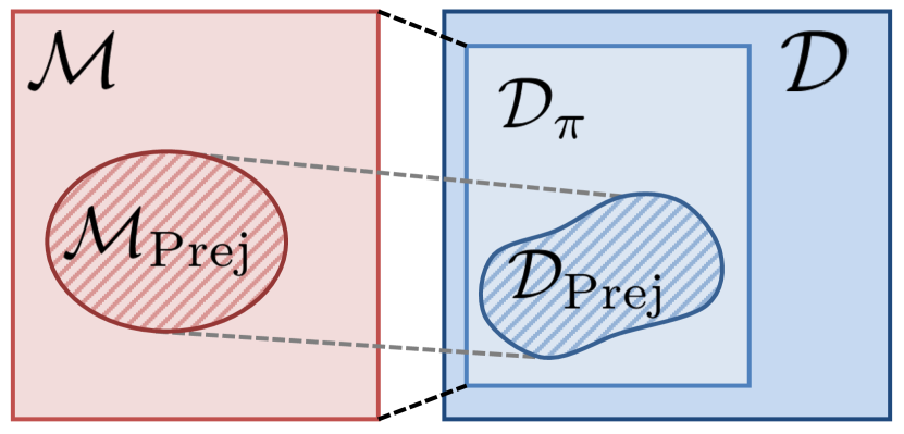
Figure 1: Cartoon of model and data spaces that we consider when thinking about how to blind an analysis, as discussed in Sect. 2.1. ${\cal M}$ is the space of all viable model parameter sets $\Theta$, which projects onto the observable-vector space ${\cal D}_{\operatorname{\pi}}\subset{\cal D}$, where ${\cal D}$ is the space of all possible observable vectors. ${\cal M}_{\operatorname{Prej}}$ is a region in parameter space associated with what we refer to as the “prejudice” distribution, describing experimenters’ preconceived expectations for where $\Theta$ is likely to be. This subset of parameter space projects onto ${\cal D}_{\operatorname{Prej}}\subset{\cal D}_{\operatorname{\pi}}$. An effective blinding transformation must have the possibility of moving the observable vector $\hat{{\mathbf{d}}}$ in or out of ${\cal D}_{\operatorname{Prej}}$ without moving it out of the prior space ${\cal D}_{\operatorname{\pi}}$.

The danger of experimenter bias arises when choices about the analysis process are made, consciously or otherwise, on the basis of whether the experiment’s results conform to the prejudices, i.e. whether $\Theta\in{\cal M}_{\operatorname{Prej}}.$ To confound the experimenter bias, a blinding procedure will apply a transformation

$$\hat{{\mathbf{d}}}\rightarrow\hat{{\mathbf{d}}}_{\rm bl}=B(\hat{{\mathbf{d}}})$$ (1)

to the data before the experimenters perform analyses. The first critical property of $B$ is therefore that it must confound the experimenter’s ability to know whether the data are consistent or inconsistent with their prejudices. For example, if we take the maximum-posterior parameter values for blinded and unblinded data

$$\Theta_{\rm unbl} =\operatorname*{argmax}_{\Theta}\left\{P\left(\Theta|\hat{{\mathbf{d}}}\right)\right\}$$ (2)

$$\Theta_{\rm bl} =\operatorname*{argmax}_{\Theta}\left\{P\left(\Theta|B(\hat{{\mathbf{d}}})\right)\right\},$$

then there must be a non-negligible chance that either

$$\operatorname{Prej}(\Theta_{\rm unbl})\gg\operatorname{Prej}(\Theta_{\rm bl})\quad\textrm{or}\quad\operatorname{Prej}(\Theta_{\rm unbl})\ll\operatorname{Prej}(\Theta_{\rm bl}).$$ (3)

A graphical illustration is given in Fig. 1: If we define ${\cal D}_{\operatorname{Prej}}$ as the region of data space ${\cal D}$ produced by parameter values within the prejudice region ${\cal M}_{\operatorname{Prej}}$, then the blinding transformation must be able to move data into and out of this region. The experimenters should believe that this is possible, but not know for certain whether it has happened. Because we are dealing with human psychology and prejudices which may not be quantifiable, we usually cannot create a strict numerical requirement to satisfy this criterion.

2.2 Criterion II: preserving the ability to check for errors

In addition to obscuring the true parameter output of an analysis, an effective blinding scheme must still allow experimenters to examine the data $\hat{{\mathbf{d}}}$, before unblinding, to uncover errors in their analysis procedure. A validation test is one whose failure indicates that data could not have been produced by any allowed parameters $\Theta\in{\cal M}$. A blinding transformation $B$ should not alter the conclusions of validation tests.

There are a number of ways of stating this requirement. Sometimes the validation tests are expressed as some projection of the data onto a “null test” $T(\hat{{\mathbf{d}}})$ such that

$$T(\hat{{\mathbf{d}}})=0\quad\forall\Theta\in{\cal M}.$$ (4)

Many kinds of validation tests fall into this paradigm. For example, if $T$ projects onto the B mode (divergence-free component) of weak lensing, it should be zero within errors. Another example is that a properly extinction-corrected galaxy survey should exhibit no statistically significant correlation between galaxy positions and star positions, so $T$ in this case would be the angular star-galaxy correlation function. Or, $T$ can measure the difference between observable vectors split by some property presumed to be uncorrelated with extra-galactic signals, such as seeing or the season when the data were collected. Another very generic test is to run the parameter inference on two subsets of the observable vector and check that the results are consistent with common $\Theta$. Allowances must of course be made for the expected noise in the null test output at fixed $\Theta$. Generally speaking, a useful blinding transformation must yield

$$T(\hat{{\mathbf{d}}}_{\rm bl})\sim 0\qquad\mbox{if and only if}\qquad T(\hat{{\mathbf{d}}})\sim 0$$ (5)

where the $\sim$ sign implies consistency with zero within measurement errors.

More generally, $B(\hat{{\mathbf{d}}})$ should map the allowed region ${\cal D}_{\operatorname{\pi}}$ onto itself, and likewise for its complement, the disallowed region $\tilde{\cal D}_{\operatorname{\pi}}$. Equivalently, the maximum-posterior values from Equations 2 should obey

$$\frac{{\cal L}\left(\hat{{\mathbf{d}}}_{\rm bl}|\Theta_{\rm bl}\right)}{{\cal L}\left(\hat{{\mathbf{d}}}_{\rm unbl}|\Theta_{\rm unbl}\right)}\approx 1.$$ (6)

In other words, blinding transformation should not significantly change the maximum likelihood in the parameter space. A transformation satisfying this requirement will ensure that blinding will not alter experimenters’ judgment about whether there are flaws in the data.

2.2.1 Model dependence of validation tests

It is important to note that defining validation tests requires one to make implicit modeling choices, and defining a blinding procedure that preserves the result of those tests can only produce shifts in parameter space that respects those choices. When constructing an analysis pipeline, it is therefore important to carefully consider what measurements will be considered results and which can be used as checks on the performance of the analysis pipeline. In other words, defining validation criteria and a blinding scheme that preserves them requires one to specify the space of models that are considered viable.

The only case in which a purely internal validation comparison can be made without reference to a model is if the exact same observable is measured twice [e.g. the amplitude of a particular cosmic microwave background (CMB) harmonic measured at a particular frequency]. Any time two distinct quantities enter the observable vector, a model is required to constrain their joint distribution. For example, suppose we compare the high- and low-redshift halves of a supernova Hubble diagram. If both halves are fit with a Lambda cold dark matter ($\Lambda$CDM) model and the data truly are from a $\Lambda$CDM universe, then analysing the two halves separately should produce consistent cosmology results, making this comparison a useful validation test. If, however, the universe is not described by $\Lambda$CDM, then the high/low $z$ split can yield inconsistent results even in the absence of processing errors. (Note that the original discovery of dark energy was effectively a demonstration that fitting supernovae data with $\Lambda=0$ produced this kind of mismatch.)

More subtly, a closer examination of the B mode null test described above (below Eq. (4)) is another demonstration of how even nominally “simple” tests can be model-dependent. Though it is true that at leading-order weak lensing in GR should have no divergence-free component, B modes can in fact be created by galaxy intrinsic alignments (IA) or modifications to GR. Thus, the test requiring measured B modes to be zero within errors can be more accurately rephrased as the requirement that the measured B modes be consistent with allowed IA and gravity models.

2.3 Criterion III: feasible implementation

Before we can begin determining the effectiveness of a blinding transformation $B$, we must first choose what data will be transformed. As a concrete example, for imaging surveys like DES the data start as pixel values, which are converted into catalogued galaxy fluxes, shapes, etc. Those catalogues are in turn converted into summary statistics such as the photometric redshift distributions $n(z)$ and tomographic weak lensing correlation functions $\xi_{\pm}(\theta)$. The summary statistics are then finally used to obtain the parameter estimates $\hat{}\Theta$ themselves.

The simplest case is simply for $B$ to operate on the $\hat{}\Theta$. As noted in Section 1, this “parameter shift” method has been used frequently, but it has the drawback of being a very thin cover over the truth. It fails, for example, if the experimenters become familiar with the relation between the observables and the cosmological parameters and are viewing how changes to the analysis impact the observables. It can also be difficult to employ this method while insuring that multiple probes are consistent with a common model. There is incentive to move the blinding transformation to an earlier stage of the analysis, where the scientists are less likely to be able to recognize whether their prejudices have been confirmed.

Blinding by alteration of the pixel data is probably impossible, apart from substituting an entire set of simulated data for the real one. Blinding at the catalogue level is possible in some cases, namely when a change in a cosmological parameter maps directly into a change in some catalogued galaxy property. For the DES Year 1 shear-only analyses (Troxel et al., 2018), all galaxy ellipticities (and hence all inferred weak lensing shears) were scaled by an unknown multiplicative factor. This is approximately equivalent to a rescaling of $\sigma_{8},$ though only in the linear regime. The possibility of catalogue-level transformations becomes remote, however, as we conduct multiprobe experiments with many correlated summary statistics, and as multiple model parameters require blinding. We have not been able to find a catalogue transformation that preserves the validity of the data for the DES combined galaxy clustering and weak lensing analysis. This has motivated us to develop an approach to blinding which relies on a transformation of the summary statistics, described in more detail below.

Recently Sellentin (2020) proposed a likelihood-level blinding via modifications of the full covariance matrix of the observable vector. It will be of interest to see if this alternative blinding method robustly satisfies criterion II from above — preserving the results of all validation tests — given that the Sellentin (2020) alteration to the covariance matrix is dependent upon the observed data.

3 Proposed method: Blinding by modifying summary statistics

Here we propose a method for consistently blinding cosmological analyses by transforming the summary statistics used as input for parameter estimation. Because parameter estimation is done by comparing measured summary statistics to theoretical predictions, the software infrastructure for an experiment will naturally include tools for computing model predictions at various points in parameter space. Our blinding transformation makes use of those tools to translate shifts in parameter space to changes in the summary statistics.

The blinding transformation works as follows. Let $\hat{d}_{i}$ be element $i$ of a measured observable vector, and let $d_{i}(\Theta)$ be the theoretically computed (noiseless) value of that same element for model parameters $\Theta$. We choose a known reference model $\Theta_{\rm ref}$ and a blinding shift $\Delta\Theta$ in the cosmological parameters. The blinding operation is then a simple modification of each element $\hat{d}_{i}$ of the observable vector,

$$B(\hat{d}_{i}) =\hat{d}_{i}+f^{\rm(add)}_{i},$$ (7)

$$f^{\rm(add)}_{i} =d_{i}\left(\Theta_{\rm ref}+\Delta\Theta\right)-d_{i}\left(\Theta_{\rm ref}\right).$$

If the expected noise level on $\hat{{\mathbf{d}}}$ does not vary much across the parameter shift $\Delta\Theta,$ then it is true by construction that $B$ will map data generated at $\Theta_{\rm obs}$ into viable data for $\Theta_{\rm bl}=\Theta_{\rm obs}+\Delta\Theta$ if the truth ($\Theta_{\rm obs}$) is sufficiently close to the reference cosmology ($\Theta_{\rm ref}$). However, because $\Theta_{\rm obs}$ is not known (in fact, this whole exercise is designed to obscure it!) and because the observable vector generally is not actually linear in parameters, it is not guaranteed that this blinding transformation will satisfy the necessary criteria for successful blinding. Its application to a given observable vector and parameter space thus requires numerical validation.

3.1 Procedure for blinding at the level of summary statistics

An overview of the procedure for summary-statistic blinding is as follows:

1. Choose a reference cosmology (and nuisance parameters) $\Theta_{\rm ref}$ in the middle of the range of models considered feasible truths.

2. Select a (blind) shift $\Delta\Theta$ from a distribution broader than the preconceptions causing the confirmation bias. For example if there is a theoretical prejudice that the dark energy equation of state parameter is $w=-1$, then $\Delta w$ should be capable of shifts four to five times the experiment’s forecasted uncertainty in $w$.

3. For each summary statistic $d_{i}$ being used for cosmological inference, calculate the blinding factor $f_{i}$ using Eq. (7).

4. Hide the real data $\hat{d}_{i}$ and give experimenters the shifted values $B(\hat{d}_{i})$ as per Eq. (7) with which to conduct all validation tests.

5. After passing validation tests, unblind by using the original unblinded data $\hat{{\mathbf{d}}}$ to repeat the inference of $\Theta.$

3.2 Evaluating performance

The blinding technique that we propose is fully described by Eq. (7). In practice, the implementation of our blinding algorithm depends on the choice of the summary statistic to which the blinding factors ${\mathbf{f}}^{\rm(add)}$ are applied, the reference parameters $\Theta_{\rm ref}$, as well as the probability distribution from which parameter shifts $\Delta\Theta$ are drawn. In order to test the performance for a given set of these choices, we must show the following:

(1) the blinding transformation is able generate shifts in best-fitting model parameters large enough to overcome experimenters’ potential biases, as described in Sect. 2.1, and

(2) the blinded observable vector $\hat{{\mathbf{d}}}_{\rm bl}$ is consistent with data that could be produced by some set of allowed model parameters, as discussed in Sect. 2.2.

We can test both of these requirements by analysing simulated data according to the procedure below.

• We choose a reasonable reference cosmology $\Theta_{\rm ref}$ as well as an ensemble of “true” parameters associated with observed unblinded data $\{\Theta_{\rm obs}^{(a)}\}$, where $a$ labels the realization. For these realizations, we also select an ensemble blinding shifts $\{\Delta\Theta^{(a)}\}$. For example, we may choose to use the reference cosmology with the dark-energy equation of state $w_{\rm ref}=-1$, and in some realization of our blinding test, we could choose $w_{\rm obs}^{(a)}=-0.875$ and $\Delta w^{(a)}=-0.031$.

• For each realization, we generate a noiseless synthetic measured observable vector by computing the theory prediction for the data at the input cosmology,

  $$\hat{{\mathbf{d}}}^{(a)}={\mathbf{d}}(\Theta_{\rm obs}^{(a)}).$$ (8)

  In our representative example above, this corresponds to, for example, a predicted weak lensing shear 2PCF evaluated at $w_{\rm obs}^{(a)}=-0.875$.

• We then blind that data vector using $\Theta_{\rm ref}$ and $\Delta\Theta^{(a)}$ according to the transformation Eq. (7) to obtain $\hat{{\mathbf{d}}}_{\rm bl}^{(a)}$. That is, we evaluate

  $$\hat{{\mathbf{d}}}_{\rm bl}^{(a)}={\mathbf{d}}(\Theta_{\rm obs}^{(a)})+{\mathbf{d}}(\Theta_{\rm ref}+\Delta\Theta^{(a)})-{\mathbf{d}}(\Theta_{\rm ref}).$$ (9)

  In our example this corresponds to the sum of the 2PCF for $w_{\rm obs}^{(a)}=-0.875$ and one for $w_{\rm ref}+\Delta w^{(a)}=-0.906$, minus the 2PCF for $w_{\rm ref}=-1$.

• By performing parameter estimation on $\hat{{\mathbf{d}}}^{(a)}$ we can find associated unblinded best-fitting parameters $\Theta_{\rm unbl}^{(a)}$. (For noiseless data we expect $\Theta_{\rm unbl}^{(a)}=\Theta_{\rm obs}^{(a)}$.) Likewise we can find the blinded best-fitting parameters $\Theta_{\rm bl}^{(a)}$ by performing parameter estimation on $\hat{{\mathbf{d}}}_{\rm bl}^{(a)}$.

Studying the distribution of these best-fitting parameters for such a simulated analyses allows us to assess the performance of the blinding transformation. Point (1) from above (that blinding must be able to produce large enough shifts in parameter space) is straightforward to check. Generally we expect that the input blinding shift will determine the shift in output best-fitting parameters,

$$\Theta_{\rm bl}-\Theta_{\rm unbl}\approx\Delta\Theta.$$ (10)

If this is true, we can ensure the blinding transformation satisfies this requirement simply by drawing $\Delta\Theta$ from a wide enough probability distribution in ${\cal M}$. By analysing an ensemble of simulated observable vectors we can explicitly check the extent to which Eq. (10) holds. It is worth noting here that it does not matter if the relation in Eq. (10) strictly holds: Blinding can still be effective as long as the output shifts $\Theta_{\rm bl}-\Theta_{\rm unbl}$ and input shifts $\Delta\Theta$ span a comparable region of parameter space.

For point (2), we propose using the quantity $\Delta\chi^{2}$, defined below, as a metric for testing whether the blinding transformation defined in Eq. (7) preserves the results of validation tests. This statistic is defined as the difference between the minimum $\chi^{2}$ for the model’s fit to blinded data and that of the fit to unblinded data:

$$\Delta\chi^{2}\equiv\left\{-2\ln{\cal L}\left(B(\hat{{\mathbf{d}}})|\Theta_{\rm bl}\right)\right\}-\left\{-2\ln{\cal L}\left(\hat{{\mathbf{d}}}|\Theta_{\rm unbl}\right)\right\}.$$ (11)

It is a measure of the extent to which blinding preserves the internal consistency of the different components of the observable vector. In other words, it quantifies how much of the error in the model’s fit to blinded data comes from the blinding procedure itself. If we can confirm that $\Delta\chi^{2}$ is sufficiently small for all realizations in our ensemble of simulated observable vectors, we can ensure that the blinding transformation satisfies Eq. (6) for the set of input parameters and blinding shifts considered.

3.3 Leading-order performance

In the context of the evaluation metric described above, a perfect blinding technique can shift the inferred parameters by the bias-defeating amount with $\Delta\chi^{2}=0,$ i.e. no change in the degree to which data obey the model. It is clear that Eq. (7) will be perfect if the data depend on the model in a purely linear fashion. Furthermore the parameter shift will be simple, i.e. Eq. (10) will attain equality.

Indeed in this linear regime with fixed covariance, blinding via Eq. (7) guarantees the more general statement that

$$\chi^{2}\left[B(\hat{{\mathbf{d}}})|\Theta_{\rm obs}+\Delta\Theta\right]=\chi^{2}(\hat{{\mathbf{d}}}|\Theta_{\rm obs}),$$ (12)

which in turn will lead to the Bayesian evidence

$$p(\hat{{\mathbf{d}}})=\int d\Theta\,{\cal L}(\hat{{\mathbf{d}}}|\Theta)p(\Theta)$$ (13)

being invariant under the blinding transformation to the extent that the prior $p(\Theta)$ is invariant under shift by $\Delta\Theta$. In this limit of fixed multivariate Gaussian noise and linear parameter shifts, the additive blinding yields data that are fully indistinguishable from a shift in the truth cosmology.

The blinding technique of Sellentin (2020) differs in that the measured observable vector $\hat{{\mathbf{d}}}$ is left unchanged, but the covariance matrix undergoes a data-dependent transformation $C_{d}\rightarrow\breve{C}_{d}(\hat{{\mathbf{d}}})$ such that the blinded $\breve{\chi}^{2}(\hat{{\mathbf{d}}}|\Theta)$ is guaranteed to satisfy

$$\breve{\chi}^{2}(\hat{{\mathbf{d}}}|\Theta_{\rm ref}+\Delta\Theta)=\chi^{2}(\hat{{\mathbf{d}}}|\Theta_{\rm ref}).$$ (14)

This is not quite the same condition as demanding $\Delta\chi^{2}=0$ in Eq. (11), since the latter operates at the best-fitting $\Theta$ in both the blinded and unblinded cases. The basic construction for $\breve{C}_{d}$ does not guarantee that the analogous property to Eq. (12) will hold, i.e. we can have

$$\breve{\chi}^{2}(\hat{{\mathbf{d}}}|\Theta+\Delta\Theta)\neq\chi^{2}(\hat{{\mathbf{d}}}|\Theta)\quad\textrm{if}\quad\Theta\neq\Theta_{\rm ref},$$ (15)

even in the linear regime. We can expect that the Sellentin (2020) blinding is functionally perfect by the definition of $\Delta\chi^{2}$ in Eq. (11) being small, for the true $\Theta$ sufficiently close to $\Theta_{\rm ref}$. Numerical investigations will be of interest to see whether covariance-matrix blinding yields sufficiently small $\Delta\chi^{2}$ over the full range of $\Theta$ allowed by any particular experiment.

Moving beyond the linear regime, in Appendix A we calculate the parameter shifts and $\Delta\chi^{2}$ induced by a quadratic dependence of data on parameters. The result is that the shift in best-fitting parameters is no longer equal to $\Delta\Theta$, but rather acquires a leading term that is linear in the product $\Delta\Theta\times\left(\Theta_{\rm obs}-\Theta_{\rm ref}\right).$ In other words we should not expect equality in Eq. (10). Keep in mind though, as we noted above, fulfilling this equality is not a goal of blinding.

The more important result is the scaling

$$\Delta\chi^{2}\sim\left|\Delta\Theta\right|^{2}\left|\Theta_{\rm obs}-\Theta_{\rm ref}\right|^{2}/\left|C\right|,$$ (16)

where $C$ is the covariance describing measurement errors on the parameters.

We can therefore expect that the blinding will succeed (by having insignificant $\Delta\chi^{2}$) within some sufficiently small region around the origin in the plane of blinding shift $\Delta\Theta$ and “truth shift” $\Theta_{\rm obs}-\Theta_{\rm ref}.$ This region must be large enough to allow the blinding shift to span ${\cal M}_{\operatorname{Prej}}$ and for the truth shift to span ${\cal M}$. Below, we will test whether this condition is met for the DES Year 3 analysis.

An important consequence of the scaling relations is that this blinding transformation will improve as our knowledge and experimental precision evolve. Let us assume that future experiments reduce measurement errors by a factor $\alpha<1$ ($C\rightarrow\alpha^{2}C$). To the extent that statistical rather than systematic uncertainties limit constraining power, the blinding shift necessary to defeat prejudices will shrink in concert ($\Delta\Theta\rightarrow\alpha\Delta\Theta$) as will the width of the priors to future experiments ($\Theta_{\rm obs}-\Theta_{\rm ref}\rightarrow\alpha(\Theta_{\rm obs}-\Theta_{\rm ref})$). Under Eq. (16) we see that $\Delta\chi^{2}\propto\alpha^{2}$ under this evolution. Hence, to the extent that these trends hold, future experiments will, in fact, become easier to blind, given the same models and observables.

4 Application: Dark Energy Survey analysis of galaxy lensing and clustering

Using the discussions in Sects. 2 and 3 as a guide, we will now test the summary-statistic blinding transformation for the DES Year 3 galaxy clustering and weak lensing combined analysis. The goal of this exercise is twofold. First, it will serve as a concrete demonstration of how summary-statistic blinding can be implemented, and secondly, we will validate the transformation’s performance for use in the DES Year 3 analysis.

DES is an imaging survey that, over the course of six years, has measured galaxy positions and shapes in a 5000 ${\rm deg}^{2}$ footprint in the southern sky. It is designed to use multiple observable probes to study the properties of dark energy and to otherwise test the standard cosmological model, $\Lambda$CDM. Those probes include galaxy clustering, weak lensing, supernovae, and galaxy clusters. Though the blinding transformation presented in this paper could be potentially useful for all of these cosmological observables, our focus in this paper is on the combined analysis of galaxy clustering and weak lensing shear.

For conciseness, we will refer to this as the $3\!\times\!2$pt analysis, so named because in it three types of 2PCF are used as summary statistics. These 2PCFs are galaxy position-position, shear-shear, and position-shear angular two-point correlations measured from DES galaxy catalogues. Additionally, we will use Year 1 (Y1) to refer to the analysis of the first year of DES data, which covers a footprint of roughly 1300 $\rm{deg}^{2}$ and for which results are reported in Dark Energy Survey Collaboration et al. (2018), and Year 3 (Y3) to refer to the ongoing analysis of the first three years of data, which will cover the full 5000 $\rm{deg}^{2}$ footprint at a similar depth.

Below, we first briefly motivate the need for blinding in DES combined-probe analyses (Sect. 4.1) before describing the $3\!\times\!2$pt data and analysis pipeline in Sects. 4.2 and 4.3. Then, Sect. 4.4 introduces our procedure for testing the performance of the 2PCF blinding transformation. Sects. 4.5 and 4.6 present the results.

4.1 The need for blinding in DES analyses

Two of the most powerful ways DES data can test the $\Lambda$CDM model are via the constraints it can place on the dark energy equation-of-state parameter $w$ and on the amplitude of matter density fluctuations $\sigma_{8}$. The equation-of-state parameter describes the ratio of pressure and density of a fluid description of dark energy in $w$CDM, an extension of $\Lambda$CDM, which describes dark energy as a fluid. If dark energy behaves as a cosmological constant (as in $\Lambda$CDM), this parameter will take the value $w=-1$, while $w\neq-1$ means that the dark energy density evolves with time. The matter density fluctuation amplitude $\sigma_{8}$ is of interest because it and $\Omega_{m}$ are the mostly precisely constrained parameters for DES’ measurements of structure in the $z\lesssim 1$ Universe. Comparing DES constraints in the $\sigma_{8}-\Omega_{m}$ plane to those extrapolated under $\Lambda$CDM from Planck CMB measurements thus tests the ability of $\Lambda$CDM to describe the evolution of the large-scale properties of the universe from early and late times. Given these tests, whether or not DES observables are consistent with the special value $w=-1$ in $w$CDM parameter space or with Planck $\Omega_{m}$-$\sigma_{8}$ results in $\Lambda$CDM are questions of particular interest for DES analyses.

The Y1-3$\times$2pt $w$CDM constraints are consistent with $w=-1$, while the $\Lambda$CDM results showed a suggestive offset from Planck in the $\Omega_{m}$-$\sigma_{8}$ plane, with the DES preferring a lower value of $\sigma_{8}$. As the Y3-3$\times$2pt analysis will use three times the sky area, that increased statistical power will cause DES constraints to tighten, and the community will be closely watching how the results compare to $w=-1$ and to the Planck $\Omega_{m}$-$\sigma_{8}$ constraints. Thus, the parameters that we are particularly interested in blinding are $w$ and $\sigma_{8}$. In the tests below, for simplicity we focus on blinding transformations shifting only those two parameters. This is sufficient to blind the DES analysis, but we do note that one could easily and reasonably adjust the transformation to include shifts in any other parameter(s) — $\Omega_{m}$, for example — in order to further confound the DES-Planck comparison.

			Parameter estimation		Distribution for blinding tests
	Parameter	$\Theta_{\rm ref}$	Search bounds	Prior	$\Theta_{\rm ref}+\Delta\Theta$	$\Theta_{\rm obs}$ [fid.]	$\Theta_{\rm obs}$ [Nuis.]
cosmology parameters	$\sigma_{8}$	0.834	[0.1, 2.0]	flat	[0.734, 0.954]	Y3 Fisher	matches fid.
	$w$	-1.0	[-2.0, -0.0]	flat	[-1.5, 0.5]	Y3 Fisher	matches fid.
	$\Omega_{m}$	0.295	[0.1, 2.0]	flat	-	Y3 Fisher	matches fid.
	$h$	0.6882	[0.2,1.0]	flat	-	Y3 Fisher	matches fid.
	$\Omega_{b}$	0.0468	[0.03, 0.07]	flat	-	-	-
	$n_{s}$	0.9676	[0.87, 1.07]	flat	-	-	-
	$\Omega_{\nu}h^{2}$	$6.155\times 10^{-4}$	[0.0006, 0.01]	flat	-	-	[0.0006,0.00322]
	$N_{\text{ massive }\nu}$	3	-	fixed	-	-	-
	$N_{\text{ massless }\nu}$	0.046	-	fixed	-	-	-
	$\tau$	0.08	-	fixed	-	-	-
lens galaxy bias	$b_{1}$	1.45	[0.8, 2.5]	flat	-	Y3 Fisher	full prior
	$b_{2}$	1.55	[0.8, 2.5]	flat	-	Y3 Fisher	full prior
	$b_{3}$	1.65	[0.8, 2.5]	flat	-	Y3 Fisher	full prior
	$b_{4}$	1.8	[0.8, 2.5]	flat	-	Y3 Fisher	full prior
	$b_{5}$	2.0	[0.8, 2.5]	flat	-	Y3 Fisher	full prior
shear calib.	$m_{1\text{--}4}$	0.012	[-0.1, 0.1]	$\mathcal{N}(0.012,0.023)$	-	-	[-0.57,0.081]
intrinsic alignments	$A_{IA}$	0.0	[-5, 5]	flat	-	-	[0,1]
	$\alpha_{IA}$	0.0	[-5, 5]	flat	-	-	[-4, 4]
	$z_{0}^{(IA)}$	0.62	-	fixed	-	-	-
source galaxy photo-$z$ bias	$\Delta z_{1}^{\rm source}$	-0.002	[-0.1,0.1]	$\mathcal{N}(-0.001,0.016)$	-	-	[-0.05, 0.046]
	$\Delta z_{2}^{\rm source}$	-0.015	[-0.1,0.1]	$\mathcal{N}(-0.019,0.013)$	-	-	[-0.054, 0.024]
	$\Delta z_{3}^{\rm source}$	0.007	[-0.1,0.1]	$\mathcal{N}(0.009,0.013)$	-	-	[-0.026, 0.04]
	$\Delta z_{4}^{\rm source}$	0.018	[-0.1,0.1]	$\mathcal{N}(-0.018,0.022)$	-	-	[-0.048, 0.84]
lens galaxy photo-$z$ bias	$\Delta z_{1}^{\rm lens}$	0.002	[-0.05, 0.05]	$\mathcal{N}(0.008,0.007)$	-	-	[-0.022, 0.026]
	$\Delta z_{2}^{\rm lens}$	0.001	[-0.05, 0.05]	$\mathcal{N}(-0.005,0.007)$	-	-	[-0.020, 0.022]
	$\Delta z_{3}^{\rm lens}$	0.003	[-0.05, 0.05]	$\mathcal{N}(0.006,0.006)$	-	-	[-0.018, 0.024]
	$\Delta z_{4}^{\rm lens}$	0.0	[-0.05, 0.05]	$\mathcal{N}(0.0,0.01)$	-	-	[-0.03, 0.03]
	$\Delta z_{5}^{\rm lens}$	0.0	[-0.05, 0.05]	$\mathcal{N}(0.0,0.01)$	-	-	[-0.03, 0.03]

Table 1: Fiducial values and prior ranges for the DES $3\!\times\!2$pt analysis pipeline studied in this work along with the range from which parameters are drawn for the blinding tests performed in this study. Fiducial values and priors are chosen to be similar to the settings for the DES Y1-3$\times$2pt analysis (with the exception of $w$, which uses a wider range here than in Dark Energy Survey Collaboration et al. (2018)), and the fact that for these tests we search over $\sigma_{8}$ rather than $A_{s}$. The columns labelled “Distribution for blinding tests” display the range from which parameters are drawn to create the realizations of synthetic data and blinding factors used for the blinding tests and are described in Sects. 4.4.1 and 4.4.1. The “Y3 Fisher” label in the $\Theta_{\rm obs}$ column refers a multivariate Gaussian, distribution with the parameter covariance estimated using a Fisher forecast, centred on the fiducial parameter values. For $\Omega_{\nu}h^{2}$, the upper bounds of its prior range and the upper bound of its “Nuis.” range correspond to $\sum m_{\nu}=0.93\text{ eV}$, and $0.3\text{ eV}$, respectively.

4.2 Observable vector and likelihood

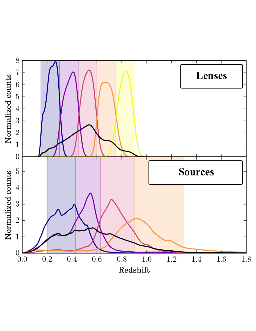
Figure 2: The $n(z)$ redshift distributions for lens and source galaxies in the DES Y1-3$\times$2pt analysis from Dark Energy Survey Collaboration et al. (2018). The vertical coloured bands show the nominal redshift range of each bin, while the lines show the estimated true redshift distribution when galaxies are binned in photometric redshift. The black lines show the unbinned total distribution. We adopt these same redshift distributions for our Y3 blinding tests.

Because the DES Y3-3$\times$2pt pipeline was not finalized when the blinding investigations presented in this paper were conducted, we approximate the Y3 observable vector and likelihood by using the Y1 modelling choices, prior ranges, and scale cuts. This section will briefly describe them, but we refer the reader to Dark Energy Survey Collaboration et al. (2018) and Krause et al. (2017) for a more detailed description of the associated measurements and calculations.

The DES $3\!\times\!2$pt analysis is based on observations of two populations of galaxies. Positions are measured for a set of lens galaxies which have been selected to have small photometric redshift (photo-$z$) errors and which have been carefully checked for residual systematics. In the Y1 analysis, this population consisted of 650,000 bright red-sequence galaxies which are selected as part of the redMaGiC catalogue (Elvin-Poole et al., 2018). Their redshift distribution is shown in the upper panel of Fig. 2. Cosmic shears are measured from a larger population of source galaxies. For the Y1 analysis the source galaxies included 26 million objects selected from the Y1 Gold catalogue (Drlica-Wagner et al., 2018) and their shapes are measured as described in Zuntz et al. (2018). The lens (source) galaxies are divided into five (four) redshift bins, respectively; see Fig. 2.

The $3\!\times\!2$pt observable vector consists of three kinds of 2PCF measured from the lens and source catalogues. The galaxy-galaxy correlations are measured as autocorrelations within each lens bin, producing a set of functions $w^{i}(\theta)$ for $i=1$–$5$. Shear-shear correlations are measured for all auto and cross-correlations of the source bins, producing functions $\xi_{+}^{ij}(\theta)$ and $\xi_{-}^{ij}(\theta)$ for $i=1$–$4$ and $1\leq j\leq i$. The galaxy-shear cross-correlations are measured between all combinations of the five lens bins and four source bins, producing $\gamma_{t}^{ij}(\theta)$ for $i=1$–$5$ and $j=1$–$4$. All of these 2PCF are measured for twenty logarithmically spaced angular bins between 2.5 and 250 arcmin. Further scale cuts are applied in order to prevent modeling uncertainties associated with non-linear structure formation, baryonic physics, and other small-scale effects from biasing the final cosmological results (Krause et al., 2017). The resulting $3\!\times\!2$pt observable vector has 457 entries.

The likelihood of the DES $3\!\times\!2$pt observable vector is modelled as a multivariate Gaussian. Its covariance $C_{{\mathbf{d}}}$ has significant off-diagonal contributions, since many elements of the observable vector can share dependence on the realization of the mass and galaxy distributions in the survey volume (also known as sample variance). We adapt the covariance matrix that was previously analytically computed for the Y1 analysis as described in Krause et al. (2017) using Cosmolike (Krause & Eifler, 2017). To approximate the Y3 covariance, we simply scale the Y1 covariance by a factor of $0.27=1350/5000$ to account for Y3’s increased survey area. This survey-area scaling correctly modifies the Gaussian parts of the covariance, but it does not properly scale the non-Gaussian contributions (Joachimi et al., 2007). Thus, this is only a rough approximation for the Y3 covariance, but it is sufficient for our testing purposes. Though, in principle, the $3\!\times\!2$pt covariance depends on the model parameters, it has been shown (Eifler et al., 2009) that the covariance’s cosmology dependence can be neglected without significantly affecting parameter constraints. In the DES Y1-3$\times$2pt analysis and in this work we do not vary the data covariance matrix when performing parameter searches.

4.3 Modelling

The parameter estimation procedure for the DES Y1-3$\times$2pt analysis, and therefore also our simulated Y3-3$\times$2pt analysis, involves a search over 27 free parameters for $w$CDM. This includes seven cosmological parameters ($\Omega_{m}$, $\sigma_{8}$, $w$, $h$, $\Omega_{b}$, $n_{s}$, and $\Omega_{\nu}h^{2}$) and 20 nuisance parameters used to account for various systematic uncertainties. These nuisance parameters include a constant linear galaxy bias $b_{i}$ for each of the five lens redshift bins. Additional nuisance parameters are introduced to model the effects of uncertainties in photo-$z$ estimation: for each lens and source bin, we introduce a parameter $\Delta z_{i}$ that describes a redshift offset of that bin’s $n(z)$ distribution. To model shear calibration, we assign one multiplicative shear calibration parameter $m_{i}$ per source galaxy bin. Following the Y1 analysis, we impose tight Gaussian external priors on all shear calibration and photo-$z$ nuisance parameters. The last set of nuisance parameters model how intrinsic (as opposed to lensing-induced) alignments between galaxy shapes affect their observed 2PCF. We use a linear alignment model with parameters $A_{IA}$, $\alpha_{IA}$, and $z_{0}^{(IA)}$. The calculations we use to compute predictions for the $3\!\times\!2$pt observable vector given this set of model parameters are described in Appendix B and in more detail in Krause et al. (2017).

The fiducial values for all of these nuisance parameters, as well as cosmological parameters, are shown in Table 1, as are the Gaussian priors used for the photo-$z$ shifts $\Delta z_{i}$ and shear calibrations $m_{i}$. During parameter estimation, the number of neutrinos $N_{\text{massive }\nu}$ and $N_{\text{massless }\nu}$ (chosen to sum to the standard model effective number of neutrinos $N_{\rm eff}$), the optical depth of the CMB $\tau$, and $z_{0}^{(IA)}$ are fixed, while the rest of the parameters shown in the table were varied with flat priors.

4.4 Evaluating performance for DES blinding

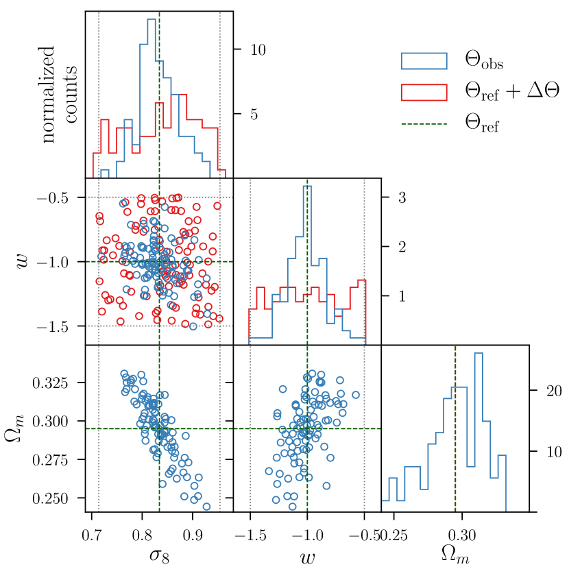
Figure 3: Values (off-diagonal panels) and the distribution (diagonal panels) of parameters $\sigma_{8}$, $w$, and $\Omega_{m}$ in the 100 realizations used for the fiducial test of our blinding procedure. The blue circles are the observed (that is true, unblinded) parameter values. The red circles are the shifted values used to blind the data. The dashed lines denote the reference model used for blinding.

Our goal is to test the performance of 2PCF-based blinding for Y3-3$\times$2pt. We do this by analysing an ensemble of 100 noiseless synthetic $3\!\times\!2$pt observable vectors. For each realization, we draw $\Delta\Theta$ (which determines the blinding transformation) and $\Theta_{\rm obs}$ (which determines the “truth” ) from probability distributions centred on a reference cosmology $\Theta_{\rm ref}$. That reference cosmology is fixed to the fiducial parameter values listed in Table 1. The synthetic “observed” data $\hat{{\mathbf{d}}}$ are then generated by computing a theory prediction for the $3\!\times\!2$pt observable vector at parameters $\Theta_{\rm obs}$, so

$$\hat{d}_{i}=d_{i}(\Theta_{\rm obs}).$$ (17)

That data are then transformed according to Eq. (7) to produce a blinded observable vector,

$$B(\hat{d}_{i})=\hat{d}_{i}+d_{i}\left(\Theta_{\rm ref}+\Delta\Theta\right)-d_{i}\left(\Theta_{\rm ref}\right).$$ (18)

We then search for parameters $\Theta_{\rm bl}$ and $\Theta_{\rm unbl}$ that maximize the likelihood (minimize $\chi^{2}$) for the blinded and unblinded data. The change $\Delta\chi^{2}$ induced by applying the blinding transformation to the data will be our measure of success for the blinding transformation, since the blinded data should look compatible with some model in the parameter space. For select realizations, we additionally study the impact of blinding on the parameter estimation posteriors, as is shown in Fig. 4. The following subsections describe the technical details of this procedure.

4.4.1 Parameter selection: fiducial test

The $\Delta\Theta$ distribution is chosen to satisfy criterion I from Sect. 2.1 above, while $\Theta_{\rm obs}$ will be drawn from a range that reasonably reflects potential offsets between the true Y3-3$\times$2pt cosmology and $\Theta_{\rm ref}$. We blind the two cosmological parameters that are at the greatest risk of experimenters’ bias in the DES $3\!\times\!2$pt analysis: the amplitude of matter clustering $\sigma_{8}$ and the dark energy equation-of-state parameter $w$. We draw $\Delta\sigma_{8}$ from a flat distribution centred on zero with bounds $-0.12<\Delta\sigma_{8}<+0.12$ chosen to be roughly equal to the $3\sigma$ errors expected from Y3-3$\times$2pt. We draw $w$ from a flat distribution $-0.5<\Delta w<+0.5$, chosen to span half of the flat prior being used for parameter estimation. All other parameters have no input blinding shift.

For our fiducial test, we vary $\Theta_{\rm obs}$ over a subset of the 27 $3\!\times\!2$pt $w$CDM parameters: $\sigma_{8}$, $w$, $\Omega_{m}$, $h$, and the five lens galaxy bias parameters $b_{i}$ for $i\in\{1,\dots,5\}$. It is drawn from a truncated multivariate Gaussian distribution in those parameters centred on $\Theta_{\rm ref}$. The covariance of that distribution is obtained from Fisher forecast for our Y3-3$\times$2pt pipeline fixing all unvaried parameters. Any realization for which $\Theta_{\rm obs}$ falls outside of the flat prior ranges in Table 1 is discarded and redrawn. Fig. 3 shows the resulting 100 realizations of $\Theta_{\rm ref}+\Delta\Theta$ and $\Theta_{\rm obs}$ for a subset of parameters.

4.4.2 $\Delta\chi^{2}$ threshold

The blinded data should appear fully consistent with having been generated by some model within ${\cal M}$ (here, $w$CDM within the priors shown in Table 1), if and only if the unblinded data are consistent with the true model. Since $\chi^{2}$ is our measure of data-model consistency, this means that we would ideally like the blinding of the data to result in $\Delta\chi^{2}=0.$ A finite $\Delta\chi^{2}$ is tolerable, however, if it is smaller than the expected statistical variation in the unblinded $\chi^{2}$, i.e. $\Delta\chi^{2}$ will not influence acceptance or rejection of the data.

We choose $\Delta\chi^{2}=30$ as a threshold for acceptable contributions from blinding to the error in the fit. This is within a few percent of the standard deviation $\sigma_{\chi^{2}}\approx\sqrt{2\nu}$ for the number of degrees of freedom $\nu$ being considered in our analyses. For comparison, in the DES Y1-3$\times$2pt analysis of Dark Energy Survey Collaboration et al. (2018) an unblinding criterion was that $\chi^{2}/\nu<1.4$. Our $\Delta\chi^{2}=30$ threshold corresponds to $\Delta\chi^{2}/\nu=0.07$.

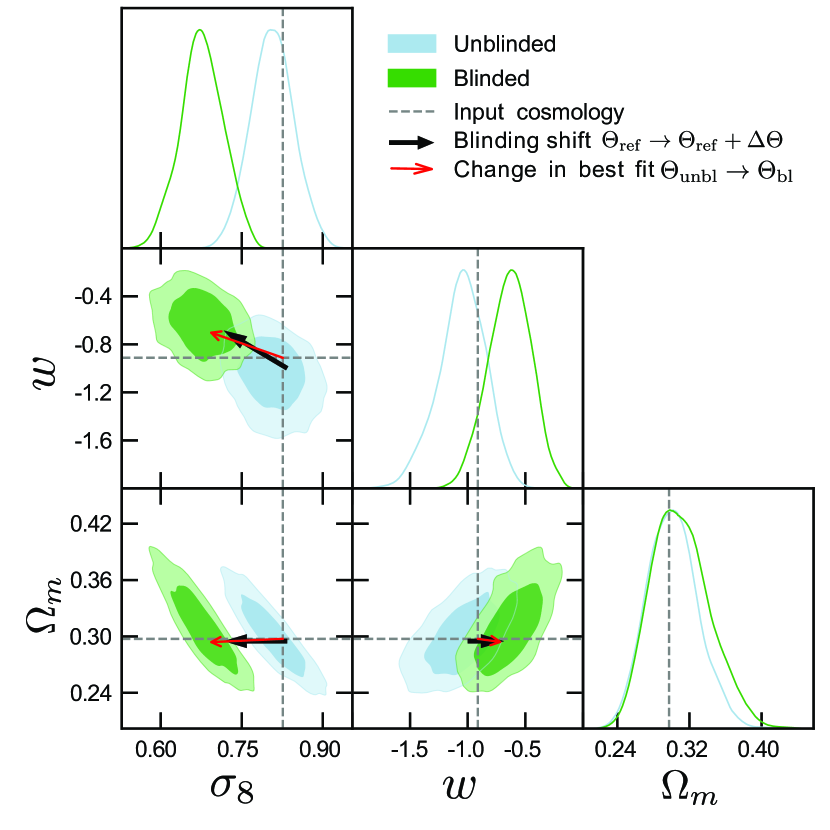
Figure 4: The 68 and 95% confidence intervals for blinded (green) and unblinded (blue) synthetic DES Y3-3$\times$2pt data. As an illustrative example, results are shown for a realization of the fiducial blinding test with a large input blinding shift of $(\Delta\sigma_{8}=-0.117,\Delta w=+0.314)$ and a low $\Delta\chi^{2}=1.86$. Dashed gray lines show the input parameters used to simulate the unblinded data $\Theta_{\rm obs}=(\sigma_{8}=0.826$, $w=-0.912$, $\Omega_{m}-0.29$). The black, thick arrow shows the points from $\Theta_{\rm ref}$ to $\Theta_{\rm ref}+\Delta\Theta$ to show the input blinding shift, and the red, thin arrow points from $\Theta_{\rm unbl}=\Theta_{\rm obs}$ to $\Theta_{\rm bl}$ to show the change in best-fitting parameters.

4.4.3 Finding the maximum likelihood

To find the best-fitting parameters, we use the Maxlike sampler in CosmoSIS, which is a wrapper for the scipy.optimize.minimize function using the Nelder-Mead Simplex algorithm (Nelder & Mead, 1965). This routine can fail to find the true maximum likelihood in high-dimensional spaces, biasing $\chi^{2}$ high. For our noise-free tests, we know $\chi^{2}=0$ for the unblinded data, hence the measured $\Delta\chi^{2}$ values are strict upper bounds on the true contributions of blinding to $\chi^{2}$. To more accurately characterise this bound, we re-run the $\chi^{2}$ minimisation search for all realizations with $\Delta\chi^{2}>30$ using the Multinest sampler (Feroz & Hobson, 2008; Feroz et al., 2009, 2013) (as implemented in CosmoSIS). Multinest is more computationally costly than Maxlike, but because it more thoroughly explores the parameter space it is less susceptible to getting stuck in local minima. We perform the Multinest searches over the full 27-dimension $w$CDM parameter space using the same low-resolution settings used for DES Y1-3$\times$2pt exploratory studies and substitute the Maxlike results with those from Multinest results in cases where the minimum $\chi^{2}$ reported from Multinest is smaller.

4.5 Results for fiducial test

Fig. 4 shows an example of how the parameter contours shift in response to a large blinding shift of $(\Delta\sigma_{8}=-0.117,\Delta w=+0.314)$. For this realization, the change in goodness of fit is small, $\Delta\chi^{2}=1.86$, and we can see that the location of the 68 and 95 percent confidence contours change in a way consistent with the input blinding shift.

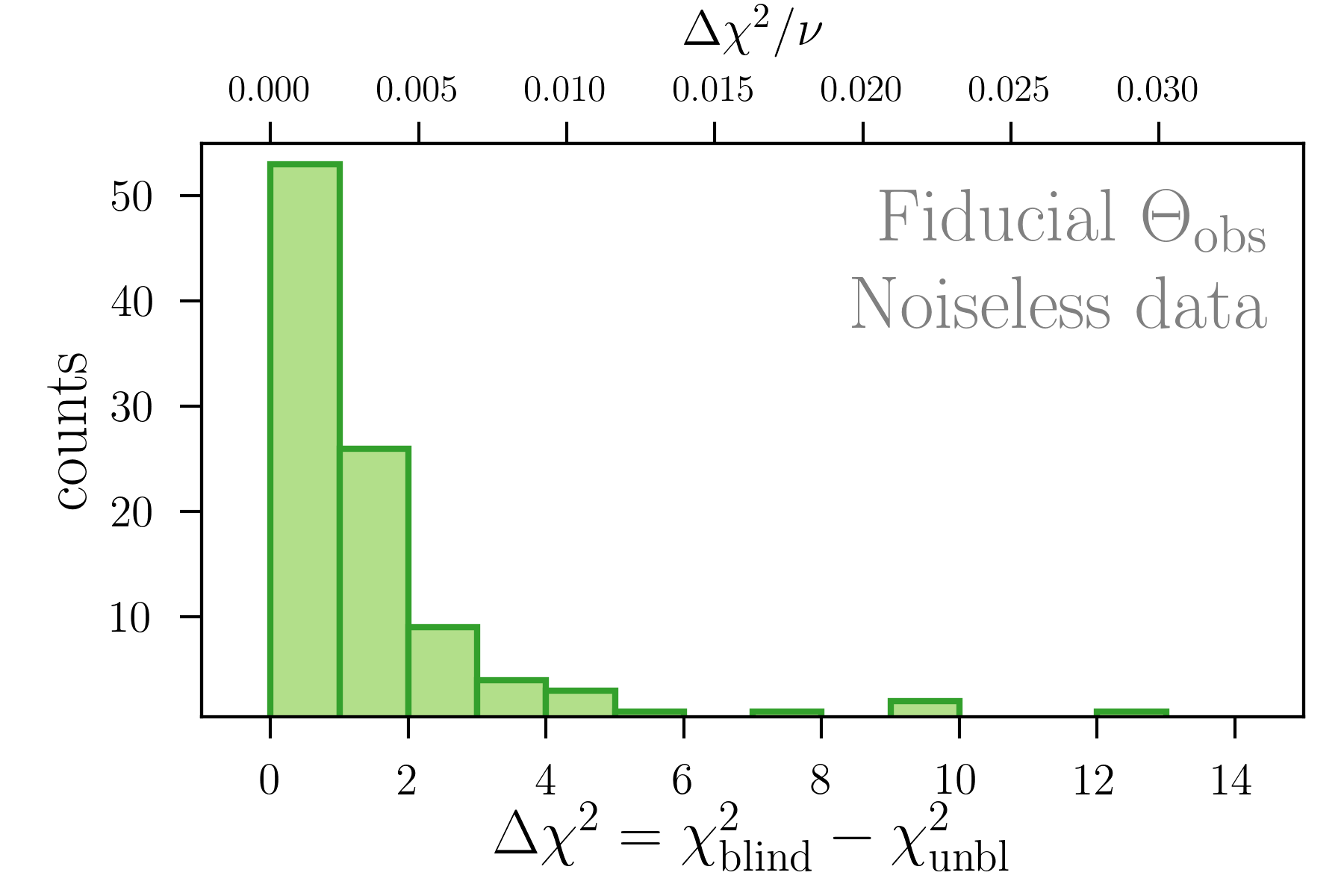
Figure 5: Fiducial blinding test results for $\Delta\chi^{2}$. The top axis shows $\Delta\chi^{2}$ in units of the degrees of freedom associated with the DES Y3-3$\times$2pt $w$CDM analysis, $\nu=430$.

More quantitatively, Fig. 5 contains the primary results for our test of the 2PCF-based blinding for the DES Y3-3$\times$2pt analysis. It shows a histogram of the $\Delta\chi^{2}$ values for the 100 blinded and unblinded pairs of synthetic observable vectors analysed. We see that in all realizations $\Delta\chi^{2}$ is well below our $\Delta\chi^{2}=30$ cut-off. This means that the blinded data are indistinguishable from unblinded data at different input parameters.

Figure 6: Dependence of $\Delta\chi^{2}$ on the magnitude of the truth shift $|\Theta_{\rm obs}-\Theta_{\rm ref}|/\sigma_{\Theta}$ (vertical axis) and of the blinding shift $|\Delta\Theta|/\sigma_{\Theta}$ (horizontal axis) for the observable vectors generated using the fiducial 100 realizations of true cosmology $\Theta_{\rm obs}$. These distances are evaluated in the two-dimensional $\sigma_{8}-w$ plane for the blinding shift and in the full 27-dimensional parameter space for the truth shift. In both cases the distance is scaled according to expected parameter uncertainties and are shown in units of the number of standard deviations for a one-dimensional Gaussian distribution with equivalent probability-to-exceed. The colours of the points represent the $\Delta\chi^{2}$ value of those realizations.

In Sect. 3.3 we suggested that the performance of the blinding transformation should worsen (higher $\Delta\chi^{2}$) when both the blinding shift $\Delta\Theta$ and the truth shift $\Theta_{\rm obs}-\Theta_{\rm ref}$ become significantly non-zero. Fig. 6 plots the $\Delta\chi^{2}$ of each fiducial realization (as the colour) vs the size of the blinding shift and the truth shift. To quantify the size of these shifts, we extract a parameter covariance $C$ from a fiducial Multinest chain and use it to compute distances in parameter space,

$$|\Theta_{\rm obs}-\Theta_{\rm ref}|/\sigma_{\Theta} =\sqrt{(\Theta_{\rm obs}-\Theta_{\rm ref})^{T}C^{-1}(\Theta_{\rm obs}-\Theta_{\rm ref})},$$ (19)

$$|\Delta\Theta|/\sigma_{\Theta} =\sqrt{(\Delta\Theta)^{T}C^{-1}(\Delta\Theta)}.$$ (20)

For the blinding shift, we compute this distance in the marginalized two-dimensional $\sigma_{8}-w$ plane (that is, we use a $2\times 2$ $C$ containing only the entries for those parameters). We evaluate the truth shift in the full 27-dimensional parameter space. For ease of interpretation, these distances are then converted into an equivalent deviation for a one-dimensional Gaussian normal distribution by equating the probability-to-exceed value: we solve for $N$ such that

$$P(\chi^{2}>N^{2},\nu=1)=P(\chi^{2}>\left(|\Delta\Theta|/\sigma_{\Theta}\right),\nu=2)$$ (21)

and likewise for the truth shift (but with $\nu=27$ on the right). For example, a truth shift of $|\Theta_{\rm obs}-\Theta_{\rm ref}|/\sigma_{\Theta}=\sqrt{30}\simeq 5.5$ that corresponds to $\chi^{2}=30$ in 27-dimensional parameter space has the same probability-to-exceed as a $\chi^{2}=1$ signal in a one-dimensional Gaussian, so we would plot this as a “$1\sigma$” blinding shift in the metric of the parameter covariance matrix.

Fig. 6 confirms the behaviour derived in Sect. 3.3 that the larger $\Delta\chi^{2}$ values appear only when both $\Theta_{\rm ref}+\Delta\Theta$ and $\Theta_{\rm obs}$ move significantly away from $\Theta_{\rm ref}$ under the metric of the experimental posterior. This trend is non-monotonic because the performance of blinding depends somewhat on the direction in parameter space of the vector $\Theta_{\rm obs}-\Theta_{\rm ref}$ in addition to its magnitude. Furthermore there is noise in our $\Delta\chi^{2}$ evaluation from imperfect optimisation.

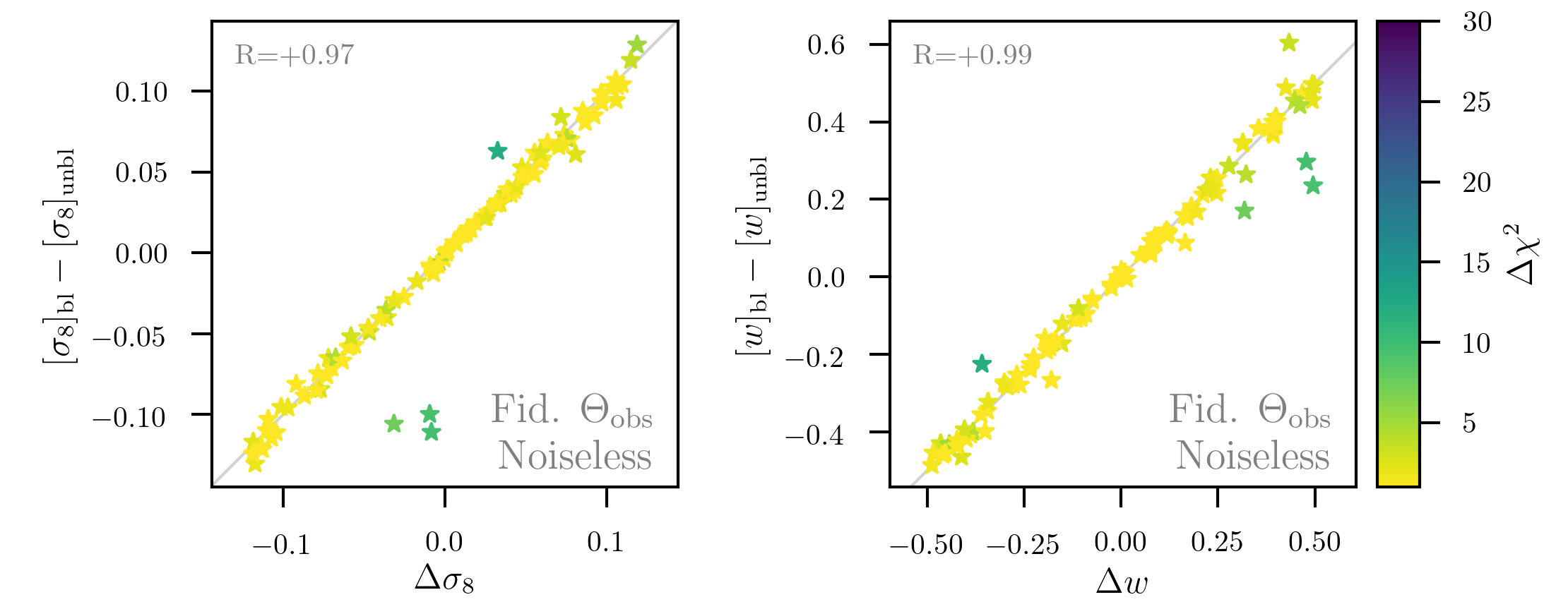
Figure 7: Relationship between the input blinding shifts (horizontal axes) in $\sigma_{8}$ (left-hand panel) and $w$ (right-hand panel) and the output shifts in best fit values of those same parameters. The colour scale shows $\Delta\chi^{2}$ and the diagonal grey line shows the case where the output shifts are exactly equal to the input shifts. Both plots show data from the same 100 realizations for noiseless simulated data.

Fig. 7 shows the relationship between the input blinding shifts in $\sigma_{8}$ and $w$ and the resulting shift in their best-fitting values. We generally find the behaviour expected from the leading-order analysis, which is for $\Theta_{\rm bl}-\Theta_{\rm unbl}$ to be roughly equal to the parameter shift $\Delta\Theta$ used to generate the blinding factors, although with some deviation that grows roughly linearly with $\Delta\Theta$. The scatter is expected because unplotted parameters, as well as the truth shift $\Theta_{\rm obs}-\Theta_{\rm ref}$, also influence the deviation. The fact that the range of the points along the veritical axes of Fig. 7 is comparable to that along the horizontal axis does confirm that this blinding transformation is capable of altering the experiment’s results enough to overcome experimenters’ potential biases. Having satisfied all of the desired criteria described in Sect. 2, we consider the blinding transformation of Eq. (7) to be successful for this fiducial analysis.

Fig. 7 can give us additional insight into the performance of our blinding transformation. In that Figure, the colour of each point corresponds to the $\Delta\chi^{2}$ value for that realization. We note that the strong outlier points are also the points with largest $\Delta\chi^{2}$. This is the expected behaviour. We saw in Fig. 6 that these high-$\Delta\chi^{2}$ realizations have large truth shifts, and we expect that larger truth shifts should induce larger differences in $\Theta_{\rm bl}-\Theta_{\rm obs}$, mediated by the non-linear portions of the data model as indicated by Eq. (27). Those differences are expected to occur for all parameters, not just those we choose to blind. We confirm from our Maxlike results that, for such outlier realizations of $\Theta_{\rm obs}$, blinding induces large changes in the best-fitting values of several nominally unblinded parameters.

To further investigate this, we additionally ran Multinest chains for those realizations. We found that in two of these realizations the 68 or 95 percent confidence intervals of posterior are pushed into the hard-prior boundary for some of the galaxy bias parameters. Such behaviour could be problematic, since checking that posterior distributions have not hit prior bounds is a standard part of data validation, and the blinding could trigger a false alarm for this. This issue not necessarily prohibitive: Since we know that this kind of unpredictable shift is occurring for realizations with large truth offsets $\Theta_{\rm obs}-\Theta_{\rm ref}$, one could imagine workarounds in the blinding procedure to account for, or protect against, this possibility. For example, the collaboration could ask a single member to confirm whether the collision with the prior bound is in fact due to the blinding shift or, as discussed in Sect. 5 below, one could make use of several distinct blinding shifts defined at different $\Theta_{\rm ref}$ values.

4.5.1 Impact of noise

As an additional check, we perform this analysis on a version of these same 100 synthetic observable vectors with Gaussian noise added using a Cholesky decomposition of the covariance $C_{{\mathbf{d}}}$. Results from this test are shown in Appendix C. Compared to the noiseless results shown above, there is slightly more scatter in the input-vs-output parameter shift relationship, and in the relationship between $\Delta\chi^{2}$ and the various input parameters. These differences are expected and do not change the conclusions that the blinding transformation is effective.

4.6 Follow-up test: varying nuisance parameters

As a stronger test of 2PCF-based blinding for the DES Y3-3$\times$2pt analysis, we analyse a second set of synthetic observable vectors for which more parameters of $\Theta_{\rm obs}$ are allowed to deviate from $\Theta_{\rm ref}$. This is a more rigorous test because it allows for larger differences between the truth model and the reference model; recall that we noted in Sect. 3.3 that we expect the performance of the blinding method to degrade as the magnitude of the difference $\Theta_{\rm obs}-\Theta_{\rm ref}$ increases. We use the same 100 blinding factors as in the fiducial test. For the 100 realizations of $\Theta_{\rm obs}$, the values of $\sigma_{8}$, $w$, $\Omega_{m}$, $h$ match those used in the fiducial test, but we additionally vary $\Omega_{\nu}h^{2}$, reselect values of galaxy bias $b_{1\text{--}5}$, and vary all remaining nuisance parameters over flat probability distributions with ranges shown in the rightmost column of Table 1. For the nuisance parameters with Gaussian priors in the $3\!\times\!2$pt analysis, the ranges are $\pm 3\sigma$ for that prior. The galaxy bias parameters are drawn from their full prior range, while the ranges for neutrino mass and intrinsic alignment parameters are chosen by eye based on the DES Y1-3$\times$2pt posteriors in Dark Energy Survey Collaboration et al. (2018). In the text and plots below we will refer to results from this test as the “nuisance” test (as opposed to fiducial test).

Figure 8: Same as Fig. 5, but for the “nuisance test” ensemble of unblinded observable vectors: histogram of $\Delta\chi^{2}$ values. The vertical dashed line shows our $\Delta\chi^{2}=30$ threshold, which is now exceeded by 4 of the 100 trials.

After searching for best-fitting parameters on the pairs of blinded and unblinded observable vectors of the nuisance test, we can study the same results discussed in Sect. 4.5. Fig. 8 shows a histogram of the $\Delta\chi^{2}$ values. Although the majority of realizations remain below $\Delta\chi^{2}<30$, the distribution is broader than in the fiducial test and four realizations exceed that threshold.

Figure 9: For the “nuisance test” ensemble, we plot the $\Delta\chi^{2}$ induced by the blinding process as the colour of each point, vs the blinding shifts applied to the two cosmological parameters of greatest interest. Points with $\Delta\chi^{2}>30$ are shown in red and are circled.

Figure 10: Same as Fig. 6, but for the “nuisance test” ensemble of unblinded observable vectors: dependence of $\Delta\chi^{2}$ on the parameter-space distances associated with $\Theta_{\rm obs}-\Theta_{\rm ref}$ and $\Delta\Theta$. Circled points shown in red are realizations with $\Delta\chi^{2}>30$.

Figure 11: Same as Fig. 7 but for the “nuisance test” ensemble of unblinded observable vectors: the relationship between input blinding shifts $\Delta\Theta$ and output shifts in best-fitting parameters $\Theta_{\rm bl}-\Theta_{\rm unbl}$. Realizations with $\Delta\chi^{2}>30$ are shown with circled red points. The grey lines correspond to equal input and output shifts.

To understand the nature of the failures, we examine how $\Delta\chi^{2}$ depends on the blinding shifts and truth shifts of each realization. Fig. 9 plots the distribution of $\Delta\chi^{2}$ values for the nuisance test in the space of blinding shifts applied to $\sigma_{8}$ and $w$. Here it is apparent that larger blinding shifts, particularly those that reduce $\sigma_{8}$, are associated with higher $\Delta\chi^{2}$. A more revealing picture is given in Fig. 10, where it is clear that the unacceptable $\Delta\chi^{2}$ trials are those with larger blinding shifts and extremely large distances between $\Theta_{\rm obs}$ and $\Theta_{\rm ref}$ (under the posterior parameter metric). Note that change of scale on the $y$ axis from Fig. 6.

In interpreting these results, we emphasize that this is by design a conservative test of the blinding transformation. The fact that the true cosmologies $\Theta_{\rm obs}$ are drawn from a flat probability distribution in a large number of nuisance parameters means that the distances shown on the vertical axis of Fig. 10 are very large relative to projected Y3-3$\times$2pt uncertainties. In other words, all of the realizations studied for the nuisance test have truth parameters that are collectively highly unlikely under the priors that have been assigned to them, and even more unlikely under the expected posterior probability. To put this in perspective, note that a more realistic simulation of the blinding transformation’s performance could be done by drawing $\Theta_{\rm obs}$ from the DES Y1-3$\times$2pt posterior probability distribution, which might be considered an appropriate prior for Y3. The resulting ensemble of $\Theta_{\rm obs}-\Theta_{\rm ref}$ separations would be significantly smaller than those used here, we would expect better performance in our $\Delta\chi^{2}$ test. However, especially given the limited number (100) of realizations, sampling $\Theta_{\rm obs}$ from the Y1 posterior would result in few realizations with large $\Theta_{\rm obs}-\Theta_{\rm ref}$ which might test the limits of this approach to blinding. In contrast, our nuisance test’s flat probability distributions and resulting extremely large truth shifts let us probe regions of parameter space where the blinding transformation breaks down. We then check that those regions are highly unlikely for the application we are considering. We conclude that, although the nuisance test has failed blinding Criterion 2 of Sect. 2.2 in 4% of our trials, this only occurs for realizations with true parameters that are much farther from our reference parameters than they would realistically be for DES Y3-3$\times$2pt.

Fig. 11 shows how blinding shifts relate to output shifts in the best-fitting parameters for the nuisance test. Compared to similar results from the fiducial test (Fig. 7) there is more scatter in this relationship and the high-$\Delta\chi^{2}$ points depart further from the trends. These behaviours are consistent with what we expect from expanding the $\Theta_{\rm obs}$ space. There is some curvature present in these relations at low $w$, which suggests that the model is extending to regions where the quadratic approximation assumed in Appendix A is inadequate. Nonetheless we still confirm that the output parameter shifts are large enough to defeat observer prejudice.

5 Discussion and Conclusions

This paper presents and demonstrates an effective blinding strategy for multiprobe cosmological analyses at the summary-statistic level, with the principal requirement that such a strategy allows for robust validation checks (e.g. inspection of the blinded observable vector for obvious systematics) while hiding the cosmological-parameter values which are eventually to be inferred.

The blinding transformation is described in Eq. (7): One simply adds the difference between two theoretically-calculated observable vectors to the measured data. The “blinding shift” is the prediction for a reference cosmology $\Theta_{\rm ref}$ subtracted from the prediction for shifted cosmology $\Theta_{\rm ref}+\Delta\Theta$. In the limit where the measurement noise is invariant and the summary statistics are linear functions of the parameters $\Theta$, this transformation will generate blinded summary statistics that are completely indistinguishable from real data generated by the same experiment at an altered set of parameters $\Theta_{\rm obs}+\Delta\Theta$, i.e. a perfect blinding. This limit may or may not hold in the region spanned by the reference parameters, the shifted parameters, and the true-sky parameters $\Theta_{\rm obs}$. In practice the model $d\left(\Theta\right)$ for the summary statistics will have non-linearity over the parameter range of interest, and one must check that the blinded data are close (in a $\chi^{2}$ sense) to data that could be generated by some valid set of parameters $\Theta_{\rm bl}.$ Therefore, most of this paper is devoted to verifying that this is the case for the forecasted DES Year 3 galaxy clustering and weak lensing, or Y3-3$\times$2pt, analysis. We also check that this blinding transformation is capable of hiding the true results of the analysis, i.e. that this transformation can change the results enough so that that knowing $\Theta_{\rm bl}$ does not allow experimenters to know how the data compare to their prejudices.

These results serve both as a concrete example of the blinding transformation and as verification that it is reliable enough to use for the real DES Y3-3$\times$2pt analysis. We focus on blinding shifts in $\sigma_{8}$ and $w$, and performed this test by finding the best-fitting parameters for blinded and unblinded versions of 100 realizations of noiseless synthetic measured observable vectors. (See Fig. 4 for an illustrative example.) In order to mimic the fact that the true cosmology will not match our fiducial $\Theta_{\rm ref}$, we vary the input parameters $\Theta_{\rm obs}$ for those simulations. For a proof-of-concept fiducial test, we select a subset of cosmologial parameters from a Fisher-forecast-based multivariate Gaussian distribution, and for a more conservative follow-up “nuisance test,” we additionally draw the values of nuisance parameters from flat probability distributions, resulting in very large $\Theta_{\rm obs}-\Theta_{\rm ref}$ offsets. The change in goodness of fit $\Delta\chi^{2}$ due to blinding serves as our principle metric for successful blinding, as it measures the extent to which blinding preserves the internal consistency of the individual observable vector components.

For the fiducial test, the impact of blinding on the goodness of fit was below the expected rms statistical fluctuations in $\chi^{2}$ for all realizations (Fig. 5), and the change in best-fitting parameters was generally well predicted by the input blinding shift (Fig. 7). As expected from the leading-order analysis for non-linear models (Sect. 3.3), the $\Delta\chi^{2}$ figure of merit for blinding scales as a power of the product of the sizes of the blinding shift $\Delta\Theta$ and the “truth shift” $\Theta_{\rm obs}-\Theta_{\rm ref}$. We also verified that those results are not significantly affected when Gaussian noise is added to the simulated data (Appendix C). We noted one potential cause for concern, in that for a small number of realizations with large truth offset $\Theta_{\rm obs}-\Theta_{\rm ref}$, the blinding transformation resulted in large changes to the best-fitting values of nominally unblinded parameters which were large enough to push the posterior into a prior boundary.

When we stress the blinding transformation with the nuisance-parameter test case, the typical $\Delta\chi^{2}$ performance worsened somewhat (Figs. 8–10). The majority of realizations in this latter test still fall below the criterion $\Delta\chi^{2}<30$ (i.e. less than the standard deviation of $\chi^{2}$), but 4 out of 100 realizations exceeded that value, indicating a poor fit of our model to the blinded data. These realization are found, however, to have input parameters $\Theta_{\rm obs}$ that are very far from the reference parameters $\Theta_{\rm ref}$ assumed for blinding, both in the sense that they would have low probability under the priors on nuisance parameters, and that they are the equivalent of $50\sigma$ unlikely for the Y3-3$\times$2pt parameter errors at $\Theta_{\rm ref}$. An appropriate choice of $\Theta_{\rm ref}$ will preclude the appearance of these high-$\Delta\chi^{2}$ cases in the real Y3-3$\times$2pt analysis.

While we have demonstrated that Eq. (7) defines a viable blinding scheme for Y3-3$\times$2pt $w$CDM analyses, it is possible that other experiments will encounter cases where the non-linearities in the data model generate unacceptably large $\Delta\chi^{2}$ over the ranges of $\Delta\Theta$ and $\Theta_{\rm obs}$ which are necessary for effective blinding over the full parameter space allowed by priors. This issue is not necessarily prohibitive, however: one can imagine additional steps in the blinding procedure to account for it (and which could potentially also be used to handle cases where prior-boundary collisions occur even with acceptably small $\Delta\chi^{2}$). For example, if all pipeline checks pass on blinded data, but the resultant $\Theta_{\rm bl}$ encroaches on the boundaries of priors on nuisance parameters, a designated member of the collaboration could look at how the posterior changes when the data are blinded using a different randomly drawn blinding shift $\Delta\Theta$. Alternatively, the person tasked with generating the blinding shifts could generate two or more $f^{\rm(add)}$ shifts that use $\Theta_{\rm ref}$ values in distinct parts of the parameter space. The collaboration’s criterion could be that the data are accepted if any one of these blinded data sets generate an acceptable $\chi^{2}$. This would allow valid data to pass when its $\Theta_{\rm obs}$ is sufficiently close to any one of the $\Theta_{\rm ref}$’s, while truly systematic errors would still be likely to fail the $\Delta\chi^{2}$ criterion. Other strategies may be viable as well.

There are a number of considerations one should take into account when deciding whether and how to adopt the summary-statistic blinding transformation described in this paper. Summary-statistic blinding has the advantage that there is relatively low overhead for implementation: it can make use of existing analysis infrastructure, since the blinding factors are computed using the same theory prediction machinery needed for parameter estimation. To make the blinding more robust, it should ideally be implemented as an automatic step when summary statistics are measured from the data. It is a trivial matter for a collaboration member to infer the blinding shifts and unblind their data, if the blinding code is freely available: All one needs to do is run a zero vector through the blinding subroutine. Thus some level of self-control and trust are still required for successful blinding—we are not proposing a foolproof cryptographic system.

It is also worth considering whether multiple stages of blinding should be adopted: Especially for a new blinding technique and new analyses, having a step of parameter-level blinding (hiding numbers on parameter constraint contours) even after unblinding the summary statistics, can be useful. It is also worth considering how to check or protect against spurious cases where this transformation may lead to undesired behaviour, like pushing an acceptable unblinded parameter values past its bound from the prior. It is also important to keep in mind that blinding necessarily adds time to an analysis and in particular that using this transformation will require MCMC chains for parameter estimation to be re-run when it is time to unblind. One can argue that this serves as a feature rather than a bug: The barrier to unblinding can help force a collaboration of busy people with divided attention to pause and consider the status of an analysis before proceeding.

This summary-statistic blinding transformation is implemented as part of the ongoing DES Y3-3$\times$2pt analysis. In practice, the blinding transformation is applied using a script that runs automatically when the 2PCF are measured from galaxy catalogues. This script uses a string seed to pseudo-randomly draw a blinding shift in parameter space, which uses the same configuration files as the parameter estimation pipeline to compute and apply blinding factors to the measured 2PCF. The same transformation will also be applied to the combined analysis of the $3\!\times\!2$pt data with CMB lensing. Looking further forward, summary statistic blinding has the potential for broad applicability to many kinds of multiprobe cosmological analyses. It would be interesting to study its applicability to summary statistics for observables beyond 2PCF, such as supernovae, galaxy cluster number counts, or spectroscopic galaxy clustering measurements.

Blinding to protect results against human bias is essential in modern observational cosmology, where complex analyses combining data from multiple observables are leveraged to make increasingly precise constraints. Whereas powerful blinding techniques had already been devised in experimental particle physics, they do not naturally translate to cosmology, particularly to multiprobe analyses that can generally not be separated into distinct “signal” and “background” domains. The blinding transformation described in this paper provides a new and promising method for blinding such analyses, which we have demonstrated is applicable to current multiprobe analyses like those being done for DES. An important property of this blinding transformation is it becomes more effective (lower $\Delta\chi^{2}$, see Sect. 3.3) as experiments evolve to higher precision and our priors and prejudices focus on smaller regions of parameter space, and non-linear components of the model shrink in comparison to the linear. This makes it a promising potential tool for future cosmological analysis. Of course, one should explicitly investigate how the performance of summary statistic blinding changes as noise on the data decreases to levels like one might expect for future surveys like DESI, LSST, Euclid, and WFIRST.

Appendix A Leading-order behaviour of blinded observable vectors

We can safely assume that the model ${\mathbf{d}}(\Theta)$ is analytic and can be expanded about the reference parameters $\Theta_{\rm ref}$ in a Taylor series. We can, without loss of generality, set $\Theta_{\rm ref}=0$ and ${\mathbf{d}}(\Theta_{\rm ref})=0$ in this section. The Taylor expansion becomes

$$d_{i}(\Theta)=d_{i,\alpha}\theta_{\alpha}+\frac{1}{2}d_{i,\alpha\beta}\theta_{\alpha}\theta_{\beta}+O\left(\theta^{3}\right),$$ (22)

where we adopt the usual conventions that repeated indices within a term indicate summation, and indices after the comma denote derivatives taken at the reference parameters. For clarity we will use Latin indices to indicate dimensions in data space, and Greek indices for parameter-space dimensions. We will also, in this section, define

$${\mathbf{s}} =\Delta\Theta$$

$${\mathbf{t}} =\Theta_{\rm obs}-\Theta_{\rm ref},$$

the latter being the true cosmology for the observed Universe. In the noise-free case, we can apply the quadratic approximation in (22) to the blinding Eq. (7) to obtain the blinded observable vector

$$\hat{d}^{\rm bl}_{i}=d_{i,\alpha}\left(s_{\alpha}+t_{\alpha}\right)+\frac{1}{2}d,_{i,\alpha\beta}\left(s_{\alpha}s_{\beta}+t_{\alpha}t_{\beta}\right).$$ (23)

We seek the best-fitting parameters $\Theta^{\rm bl}$ by minimizing the $\chi^{2}$ of the solution:

$$\chi^{2}\left(\Theta^{\rm bl}\right)=\left[\hat{d}^{\rm bl}_{i}-d_{i}\left({\Theta^{\rm bl}}\right)\right]F_{ij}\left[\hat{d}^{\rm bl}_{j}-d_{j}\left({\Theta^{\rm bl}}\right)\right],$$ (24)

where we define $F=C_{{\mathbf{d}}}^{-1}$ to be the inverse of the observational covariance matrix. We take $F$ to be independent of the model parameters. In the linear limit it is easy to see that the blinding shift is always exact, $\Theta^{\rm bl}={\mathbf{s}}+{\mathbf{t}},$ so we introduce the correction term $\tilde{\theta}$ such that

$$\tilde{\theta}=\Theta^{\rm bl}-{\mathbf{s}}-{\mathbf{t}}.$$ (25)

With this definition, we can write the data differential to leading order in each of $\tilde{\theta},s,$ and $t$ as

$$\hat{d}^{\rm bl}_{i}-d_{i}\left({\Theta^{\rm bl}}\right)\approx-d_{i,\alpha}\tilde{\theta}_{\alpha}-d_{i,\alpha\beta}\left[s_{\alpha}t_{\beta}+\tilde{\theta}_{\alpha}\left(s_{\beta}+t_{\beta}\right)+\frac{1}{2}\tilde{\theta}_{\alpha}\tilde{\theta}_{\beta}\right].$$ (26)

Upon substituting this Taylor expansion back into (24), we can find the blinding shift adjustment $\tilde{\theta}$ that yields the minimal $\chi^{2}$. Again retaining only leading-order terms in $\tilde{\theta},s,$, and $t$:

$$\tilde{\theta}_{i} \approx-\left(D^{T}FD\right)^{-1}D^{T}C_{{\mathbf{d}}}^{-1}{\mathbf{q}}$$ (27)

$$\begin{split}\Delta\chi^{2}&\approx\left(P{\mathbf{q}}\right)^{T}C_{{\mathbf{d}}}^{-1}\left(P{\mathbf{q}}\right)\\ &\leq{\mathbf{q}}^{T}C_{{\mathbf{d}}}^{-1}{\mathbf{q}}\end{split}$$ (28)

where we have defined the first derivative matrix and the quadratic data perturbation respectively as

$$D_{i\alpha} \equiv d_{i,\alpha}$$

$$q_{i} \equiv d_{i,\alpha\beta}s_{\alpha}t_{\beta}.$$

$P$ is a projection matrix that removes the portion of the non-linear data shift ${\mathbf{q}}$ which can be fitted by a shift in parameters:

$$P\equiv I-D\left(D^{T}FD\right)^{-1}D^{T}C_{{\mathbf{d}}}^{-1}.$$ (29)

From these equations, several properties of the additive blinding transformation are apparent. First, the transformation is exact, in the sense that $\Delta\chi^{2}=0,$ in any of the following conditions:

1. The blinding shift ${\mathbf{s}}=\Delta\Theta$ is zero.

2. The true cosmology equals the reference cosmology, ${\mathbf{t}}=\Theta_{\rm obs}-\Theta_{\rm ref}=0.$

3. The model is linear, $d_{i,\alpha\beta}=0.$

4. The derivative matrix is invertible, in which case the projector matrix $P=0$, because any point in data space can be fit exactly with proper choice of parameters, at least locally.

Secondly, we see that a quadratic term in the data model leads to a deviation $\tilde{\theta}$ between the naive blinded cosmology parameters estimate $\Theta^{\rm bl}=\Theta_{\rm obs}+\Delta\Theta$ which scales as the product of the blinding shift ${\mathbf{s}}$ and the “truth shift” ${\mathbf{t}}.$

Thirdly, the $\Delta\chi^{2}$ in a quadratic approximation to the data model will scale as the product of the squares of the two shifts, and inversely with the measurement covariance matrix $C_{{\mathbf{d}}}$, $\Delta\chi^{2}\propto s^{2}t^{2}/C_{{\mathbf{d}}}.$ The constant of proportionality will depend on the relations between the directions of the blinding shift, the truth shift, the curvature of the model, and the covariance matrix of the observations. If we include terms beyond quadratic in the data model, we will find the dependence of $\Delta\chi^{2}$ is of even higher order in $st.$

Appendix B Modelling for 3x2pt observable vector

The theory predictions for the $3\!\times\!2$pt observable vectors are computed as follows. First, the non-linear matter power spectrum $P(k,z)$ is computed using a combination of CAMB (Lewis et al., 2000; Howlett et al., 2012) and halofit (Takahashi et al., 2012). Then, using the Limber approximation, we integrate to obtain the angular power spectra between the sets of tracers we are studying. For the correlation between the $i$th redshift bin of tracer $A$ and the $j$th bin of tracer $B$ the angular power spectrum is

$$C_{AB}^{ij}(\ell)=\left.\int\,dz\frac{H(z)}{c\,\chi^{2}(z)}W^{i}_{A}(z)W^{j}_{B}(z)P(k,z)\right|_{k=(\ell+\tfrac{1}{2})/\chi(z)},$$ (30)

where $\chi$ is the comoving radial distance and the weight functions for galaxy number density $g$ and weak lensing convergence $\kappa$ are defined as

$$W^{i}_{g}(z,k) =n_{i}(z)\,b_{i},$$ (31)

$$\begin{split}W^{i}_{\kappa}(z)&=\left(\frac{3H_{0}^{2}\Omega_{m}}{2c}\right)\left(\frac{\chi(z)}{a(z)\,H(z)}\right)\\ &\times\int_{z}^{\infty}dz^{\prime}n_{i}(z^{\prime})\frac{\chi(z^{\prime})-\chi(z)}{\chi(z^{\prime})}.\end{split}$$ (32)

Here $n_{i}(z)$ is the normalised redshift distribution and $b_{i}$ is the galaxy bias of galaxies in bin $i$. We then perform Fourier transformations to convert these angular spectra into real-space angular correlation functions, which can be compared to data. The galaxy-galaxy correlation is

$$w^{ij}(\theta)=\sum_{\ell}\frac{2\ell+1}{4\pi}P_{\ell}(\cos{\theta})\,C_{gg}^{ij}(\ell),$$ (33)

where $P_{\ell}(x)$ is a Legendre polynomial of order $\ell$. In the flat-sky approximation, where sums over spherical harmonics are converted to two-dimensional Fourier modes, the predicted angular correlations between the shears of galaxies in tomographic bins $i$ and $j$ are

$$\xi_{+}^{ij}(\theta) =\int\frac{d\ell\,\ell}{2\pi}J_{0}(\ell\theta)\,C_{\kappa\kappa}^{ij}(\ell),$$ (34)

$$\xi_{-}^{ij}(\theta) =\int\frac{d\ell\,\ell}{2\pi}J_{4}(\ell\theta)\,C_{\kappa\kappa}^{ij}(\ell),$$ (35)

$$\gamma_{t}^{ij}(\theta) =\int\frac{d\ell\,\ell}{2\pi}J_{2}(\ell\theta)\,C_{g\kappa}^{ij}(\ell),$$ (36)

where $J_{m}(x)$ is a Bessel function of the first kind of order $m$. In practice these calculations are done using the function tpstat_via_hankel: from the nicaea software (Kilbinger et al., 2009).

Nuisance parameters are included as follows. The photo-$z$ bias parameters $\Delta z_{i}^{x}$, where $x=$source or lens, have the effect of shifting the redshift distributions of the samples of galaxies:

$$n^{x}_{i}(z)\quad\rightarrow\quad n^{x}_{i}(z-\Delta z^{x}_{i})$$ (37)

Shear calibration parameters $m$ are defined so the measured shear for a galaxy is $\gamma_{\rm meas}=(1+m)\gamma_{\rm true}$. They modify the 2PCF involving source galaxies via

$$\xi_{\pm}^{ij}(\theta) \rightarrow(1+m_{i})(1+m_{j})\xi_{\pm}^{ij}(\theta),\quad\text{ and }$$ (38)

$$\gamma_{t}^{ij}(\theta) \rightarrow(1+m_{j})\gamma_{t}^{ij}(\theta).$$ (39)

The linear intrinsic alignment model used in our analysis modifies the shear convergence weight function (Eq. (32)) via

$$W^{i}_{\kappa}(z)\rightarrow W^{i}_{\kappa}(z)-\left[A_{IA}\left(\frac{1+z}{1+z_{0}}\right)^{\alpha_{IA}}\frac{C_{1}\rho_{m0}}{D(z)}\right]\frac{dn^{i}}{dz},$$ (40)

where $C_{1}=0.0134/\rho_{\rm crit}$ is a normalisation constant calibrated based on previous observations (Bridle & King, 2007).

Appendix C Additional results for noisy data

We performed a variation of our fiducial test with noisy measured observable vectors. Here we used the same true cosmology $\Theta_{\rm obs}$ and blinding shifts $\Delta\Theta$ as in Sect. 4.5. The only difference is that after computing the theory prediction at $\Theta_{\rm obs}$ to generate a synthetic measured observable vector, we added a realization of Gaussian noise produced using a Cholesky decomposition of the covariance $C_{{\mathbf{d}}}$.

Results for the noise-added version of our fiducial test are shown here. Fig. 12 shows a histogram of the resulting $\Delta\chi^{2}$ values. Fig. 13 shows how $\Delta\chi^{2}$ depends on the magnitude of the distances in parameter space associated with the blinding shift $\Delta\Theta$ and the difference between the true cosmology and that assumed for blinding $\Theta_{\rm obs}-\Theta_{\rm ref}$. There is more scatter in the relations, but otherwise the results for this test are not substantially different from those shown for the noiseless test presented in Sect. 4.5. We additionally confirmed for a few realizations that adding noise to the observable vector does not significantly change how blinding affects posterior contours like those shown in Fig. 4.

Figure 12: Same as Fig. 5, but with Gaussian noise added to the fiducial ensemble of unblinded observable vectors: histogram of $\Delta\chi^{2}$ values.

Figure 13: Same as Fig. 6, but with Gaussian noise added to the ensemble of unblinded observable vectors: dependence of $\Delta\chi^{2}$ on the parameter-space distances associated with $\Theta_{\rm obs}-\Theta_{\rm ref}$ and $\Delta\Theta$.

Affiliations

¹ Kavli Institute for Particle Astrophysics & Cosmology, P. O. Box 2450, Stanford University, Stanford, CA 94305, USA
² Department of Physics, University of Michigan, Ann Arbor, MI 48109, USA
³ Department of Physics and Astronomy, University of Pennsylvania, Philadelphia, PA 19104, USA
⁴ Department of Physics & Astronomy, University College London, Gower Street, London, WC1E 6BT, UK
⁵ Max Planck Institute for Astrophysics, Karl-Schwarzschild-Stra. 1. 85748 Garching, Germany
⁶ Department of Astronomy/Steward Observatory, University of Arizona, 933 North Cherry Avenue, Tucson, AZ 85721-0065, USA
⁷ SLAC National Accelerator Laboratory, Menlo Park, CA 94025, USA
⁸ Fermi National Accelerator Laboratory, P. O. Box 500, Batavia, IL 60510, USA
⁹ Instituto de Fisica Teorica UAM/CSIC, Universidad Autonoma de Madrid, 28049 Madrid, Spain
¹⁰ LSST, 933 North Cherry Avenue, Tucson, AZ 85721, USA
¹¹ Physics Department, 2320 Chamberlin Hall, University of Wisconsin-Madison, 1150 University Avenue Madison, WI 53706-1390
¹² CNRS, UMR 7095, Institut d’Astrophysique de Paris, F-75014, Paris, France
¹³ Sorbonne Universités, UPMC Univ Paris 06, UMR 7095, Institut d’Astrophysique de Paris, F-75014, Paris, France
¹⁴ Centro de Investigaciones Energéticas, Medioambientales y Tecnológicas (CIEMAT), Madrid, Spain
¹⁵ Laboratório Interinstitucional de e-Astronomia - LIneA, Rua Gal. José Cristino 77, Rio de Janeiro, RJ - 20921-400, Brazil
¹⁶ Department of Astronomy, University of Illinois at Urbana-Champaign, 1002 W. Green Street, Urbana, IL 61801, USA
¹⁷ National Center for Supercomputing Applications, 1205 West Clark St., Urbana, IL 61801, USA
¹⁸ Institut de Física d’Altes Energies (IFAE), The Barcelona Institute of Science and Technology, Campus UAB, 08193 Bellaterra (Barcelona) Spain
¹⁹ INAF-Osservatorio Astronomico di Trieste, via G. B. Tiepolo 11, I-34143 Trieste, Italy
²⁰ Institute for Fundamental Physics of the Universe, Via Beirut 2, 34014 Trieste, Italy
²¹ Observatório Nacional, Rua Gal. José Cristino 77, Rio de Janeiro, RJ - 20921-400, Brazil
²² Department of Physics, IIT Hyderabad, Kandi, Telangana 502285, India
²³ Excellence Cluster Origins, Boltzmannstr. 2, 85748 Garching, Germany
²⁴ Faculty of Physics, Ludwig-Maximilians-Universität, Scheinerstr. 1, 81679 Munich, Germany
²⁵ Jet Propulsion Laboratory, California Institute of Technology, 4800 Oak Grove Dr., Pasadena, CA 91109, USA
²⁶ Santa Cruz Institute for Particle Physics, Santa Cruz, CA 95064, USA
²⁷ Institut d’Estudis Espacials de Catalunya (IEEC), 08034 Barcelona, Spain
²⁸ Institute of Space Sciences (ICE, CSIC), Campus UAB, Carrer de Can Magrans, s/n, 08193 Barcelona, Spain
²⁹ Kavli Institute for Cosmological Physics, University of Chicago, Chicago, IL 60637, USA
³⁰ Department of Astronomy, University of Michigan, Ann Arbor, MI 48109, USA
³¹ Department of Physics, Stanford University, 382 Via Pueblo Mall, Stanford, CA 94305, USA
³² Department of Physics, ETH Zurich, Wolfgang-Pauli-Strasse 16, CH-8093 Zurich, Switzerland
³³ Center for Astrophysics $|$ Harvard & Smithsonian, 60 Garden Street, Cambridge, MA 02138, USA
³⁴ Australian Astronomical Optics, Macquarie University, North Ryde, NSW 2113, Australia
³⁵ Lowell Observatory, 1400 Mars Hill Rd, Flagstaff, AZ 86001, USA
³⁶ George P. and Cynthia Woods Mitchell Institute for Fundamental Physics and Astronomy, and Department of Physics and Astronomy, Texas A&M University, College Station, TX 77843, USA
³⁷ Department of Astrophysical Sciences, Princeton University, Peyton Hall, Princeton, NJ 08544, USA
³⁸ Institució Catalana de Recerca i Estudis Avançats, E-08010 Barcelona, Spain
³⁹ Department of Physics and Astronomy, Pevensey Building, University of Sussex, Brighton, BN1 9QH, UK
⁴⁰ School of Physics and Astronomy, University of Southampton, Southampton, SO17 1BJ, UK
⁴¹ Computer Science and Mathematics Division, Oak Ridge National Laboratory, Oak Ridge, TN 37831
⁴² Institute of Cosmology and Gravitation, University of Portsmouth, Portsmouth, PO1 3FX, UK
⁴³ Department of Physics, Duke University Durham, NC 27708, USA
⁴⁴ Cerro Tololo Inter-American Observatory, National Optical Astronomy Observatory, Casilla 603, La Serena, Chile
⁴⁵ Max Planck Institute for Extraterrestrial Physics, Giessenbachstrasse, 85748 Garching, Germany
⁴⁶ Universitäts-Sternwarte, Fakultät für Physik, Ludwig-Maximilians Universität München, Scheinerstr. 1, 81679 München, Germany
⁴⁷ Institute for Astronomy, University of Edinburgh, Edinburgh EH9 3HJ, UK

References

- Arisaka et al. (1993) Arisaka, K., et al., 1993, Phys. Rev. Lett., 70, 1049
- Betoule et al. (2014) Betoule, M., et al., 2014, Astron. Astrophys., 568, A22, arXiv:1401.4064
- Blake et al. (2016) Blake, C., et al., 2016, Mon. Not. Roy. Astron. Soc., 456, 3, 2806, arXiv:1507.03086
- Bridle & King (2007) Bridle, S., King, L., 2007, New J. Phys., 9, 444, arXiv:0705.0166
- Conley et al. (2006) Conley, A. J., et al., 2006, Astrophys. J., 644, 1, arXiv:astro-ph/0602411
- Dark Energy Survey Collaboration et al. (2018) Dark Energy Survey Collaboration, T., Abbott, et al., 2018, Phys. Rev., D98, 4, 043526, arXiv:1708.01530
- Dark Energy Survey Collaboration et al. (2019) Dark Energy Survey Collaboration, T., Abbott, et al., 2019, Astrophys. J., 872, 2, L30, arXiv:1811.02374
- Drlica-Wagner et al. (2018) Drlica-Wagner, A., Sevilla-Noarbe, I., Rykoff, E. S., et al., 2018, Astrophys. J. Suppl., 235, 2, 33, arXiv:1708.01531
- Eifler et al. (2009) Eifler, T., Schneider, P., Hartlap, J., 2009, Astron. Astrophys., 502, 721, arXiv:0810.4254
- Elvin-Poole et al. (2018) Elvin-Poole, J., Crocce, M., Ross, A., et al., 2018, Phys. Rev., D98, 4, 042006, arXiv:1708.01536
- Feroz & Hobson (2008) Feroz, F., Hobson, M. P., 2008, Mon. Not. Roy. Astron. Soc., 384, 449, arXiv:0704.3704
- Feroz et al. (2009) Feroz, F., Hobson, M. P., Bridges, M., 2009, Mon. Not. Roy. Astron. Soc., 398, 1601, arXiv:0809.3437
- Feroz et al. (2013) Feroz, F., Hobson, M. P., Cameron, E., Pettitt, A. N., 2013, arXiv:1306.2144, arXiv:1306.2144
- Hamana et al. (2020) Hamana, T., et al., 2020, Publ. Astron. Soc. Jap., 72, 1, Publications of the Astronomical Society of Japan, Volume 72, Issue 1, February 2020, 16, https://doi.org/10.1093/pasj/psz138, arXiv:1906.06041
- Handley & Lemos (2019) Handley, W., Lemos, P., 2019, Phys. Rev., D100, 4, 043504, arXiv:1902.04029
- Heymans et al. (2012) Heymans, C., et al., 2012, Mon. Not. Roy. Astron. Soc., 427, 146, arXiv:1210.0032
- Hildebrandt et al. (2017) Hildebrandt, H., et al., 2017, Mon. Not. Roy. Astron. Soc., 465, 1454, arXiv:1606.05338
- Howlett et al. (2012) Howlett, C., Lewis, A., Hall, A., Challinor, A., 2012, JCAP, 1204, 027, arXiv:1201.3654
- Hunter (2007) Hunter, J. D., 2007, Computing in Science & Engineering, 9, 90
- Joachimi et al. (2007) Joachimi, B., Schneider, P., Eifler, T., 2007, Astron. Astrophys., [Astron. Astrophys.477,43(2008)], arXiv:0708.0387
- Jones et al. (2001–) Jones, E., Oliphant, T., Peterson, P., et al., 2001–, SciPy: Open source scientific tools for Python, [Online; accessed 2019]
- Kilbinger et al. (2009) Kilbinger, M., et al., 2009, Astron. Astrophys., 497, 677, arXiv:0810.5129
- Klein & Roodman (2005) Klein, J. R., Roodman, A., 2005, Ann. Rev. Nucl. Part. Sci., 55, 141
- Kowalski et al. (2008) Kowalski, M., et al., 2008, Astrophys. J., 686, 749, arXiv:0804.4142
- Krause et al. (2017) Krause, E., Eifler, E., Zuntz, J., Friedrich, O., Troxel, M., et al., 2017, Submitted to: Phys. Rev. D, arXiv:1706.09359
- Krause & Eifler (2017) Krause, E., Eifler, T., 2017, Mon. Not. Roy. Astron. Soc., 470, 2, 2100, arXiv:1601.05779
- Kuijken et al. (2015) Kuijken, K., et al., 2015, Mon. Not. Roy. Astron. Soc., 454, 4, 3500, arXiv:1507.00738
- Lewis (2019) Lewis, A., 2019, GetDist: MCMC sample analysis, plotting and GUI
- Lewis et al. (2000) Lewis, A., Challinor, A., Lasenby, A., 2000, Astrophys. J., 538, 473, arXiv:astro-ph/9911177
- Nelder & Mead (1965) Nelder, J. A., Mead, R., 1965, Comput. J., 7, 308
- Oliphant (2006) Oliphant, T. E., 2006, A guide to NumPy, Trelgol Publishing, USA
- Rubin et al. (2015) Rubin, D., et al., 2015, Astrophys. J., 813, 2, 137, arXiv:1507.01602
- Sellentin (2020) Sellentin, E., 2020, Mon. Not. Roy. Astron. Soc., 492, 3, 3396, arXiv:1910.08533
- Suyu et al. (2013) Suyu, S. H., et al., 2013, Astrophys. J., 766, 70, arXiv:1208.6010
- Suyu et al. (2017) Suyu, S. H., et al., 2017, Mon. Not. Roy. Astron. Soc., 468, 3, 2590, arXiv:1607.00017
- Suzuki et al. (2012) Suzuki, N., et al., 2012, Astrophys. J., 746, 85, arXiv:1105.3470
- Takahashi et al. (2012) Takahashi, R., Sato, M., Nishimichi, T., Taruya, A., Oguri, M., 2012, Astrophys. J., 761, 152, arXiv:1208.2701
- Troxel et al. (2018) Troxel, M. A., MacCrann, N., Zuntz, J., et al., 2018, Phys. Rev., D98, 4, 043528, arXiv:1708.01538
- von der Linden et al. (2014) von der Linden, A., et al., 2014, Mon. Not. Roy. Astron. Soc., 439, 1, 2, arXiv:1208.0597
- Zhang et al. (2017) Zhang, B. R., Childress, M. J., Davis, T. M., et al., 2017, Mon. Not. Roy. Astron. Soc., 471, 2, 2254, arXiv:1706.07573
- Zuntz et al. (2015) Zuntz, J., Paterno, M., Jennings, E., et al., 2015, Astron. Comput., 12, 45, arXiv:1409.3409
- Zuntz et al. (2018) Zuntz, J., Sheldon, E., Samuroff, S., et al., 2018, Mon. Not. Roy. Astron. Soc., 481, 1, 1149, arXiv:1708.01533