Modified Cosmology Models from Thermodynamical Approach

Abstract

We apply the first law of thermodynamics to the apparent horizon of the universe with the power-law corrected and non-extensive Tsallis entropies rather than the Bekenstein-Hawking one. We examine the cosmological properties in the two entropy models by using the CosmoMC package. In particular, the first numerical study for the cosmological observables with the power-law corrected entropy is performed. We also show that the neutrino mass sum has a non-zero central value with a relaxed upper bound in the Tsallis entropy model comparing with that in the $\Lambda$CDM one.

I Introduction

According to the current cosmological observations, our universe is experiencing a late time accelerating expansion. Although the $\Lambda$CDM model can describe the accelerating universe by introducing dark energy Amendola:2015 , it fails to solve the cosmological constant problem, related to the “fine-tuning” Weinberg:1988cp ; Weinberg:1972 and “coincidence” ArkaniHamed:2000tc ; Peebles:2002gy puzzles. A lot of efforts have been made to understand these issues. For example, one can modify the gravitational theory to obtain viable cosmological models with dynamical dark energy to explain the accelerating universe Copeland:2006wr .

On the other hand, one can reconstruct the Friedmann equations through the implications of thermodynamics. It has been shown that the Einstein’s equations can be derived by considering the Clausius’ relation of a local Rindler observer  Jacobson:1995ab . In particular, this idea has been applied to cosmology, while the Friedmann equations have been obtained by using the first law of thermodynamics in the horizon of the universe Cai:2005ra . It has been also demonstrated that the modified Friedmann equations can be acquired from the thermodynamical approach by just replacing the entropy-area relation with a proper one in a wide variety of gravitational theories Cai:2005ra ; Akbar:2006er ; Akbar:2006kj ; Jamil:2009eb ; Fan:2014ala ; Gim:2014nba . Thus, as long as there is a new entropy area relation, thermodynamics gives us a new way to determine the modified Friedmann equations without knowing the underlying gravitational theory. Furthermore, since the entropy area relation obtained from the modified gravity theory can be useful to extract the dark energy dynamics along with the modified Friedmann equations, it is reasonable to believe that even if we do not know the underlying theory of modified gravity, some modifications of the entropy relation will still give us additional information for modified Friedmann equations as well as the dynamics of dark energy, which would be different from $\Lambda$CDM. As a result, we expect that the modification of the entropy is also relevant to the cosmological evolutions.

It is known that a power-law corrected term from the quantum entanglement can be included in the black hole entropy near its horizon Das:2007mj . Interestingly, one can apply it to cosmology by taking it as the entropy on the horizon of the universe. On the other hand, the universe is regarded as a non-extensive thermodynamical system, so the Boltmann-Gibbs entropy should be generalized to a non-extensive quantity, the Tsallis entropy, while the standard one can be treated as a limit Tsallis:1987eu ; Lyra:1998wz ; Wilk:1999dr . The Tsallis entropy has been widely discussed in the literature. In the entropic-cosmology scenario Easson:2010av , the Tsallis entropy model predicts a decelerating and accelerating universe Komatsu:2013qia . In addition, a number of works on the Tsallis holographic dark energy have been proposed and investigated Abreu:2014ara . In addition, the Tsallis entropy has also been used in many different dark energy models, such as the Barboza-Alcaniz and Chevalier-Polarski-Linder parametric dark energy and Wang-Meng and Dalal vacuum decay models Nunes:2014jra . Moreover, it is shown that modified cosmology from the first law of thermodynamics with varying-exponent Tsallis entropy can provide a description of both inflation and late-time acceleration with the same parameter choices Nojiri:2019skr . In particular, the Tsallis entropy is proportional to a power of the horizon area, i.e. $S_{T}\propto A^{\delta}$, when the universe is assumed to be a spherically symmetric system  Tsallis:2012js .

Although it is possible to modify Friedmann equations by just considering fluid with an inhomogeneous equation of state of the corresponding form 1205.3421 , we still choose the thermo-dynaimical approach as that in Ref. Lymperis:2018iuz , in which the authors considered the first law of thermodynamics of the universe with fixed-exponent Tsallis entropy and showed that the cosmological evolution mimics that of $\Lambda$CDM and are in great agreement with Supernovae type Ia observational data. In this paper, we examine the features of the modified Friedmann equations obtained by replacing the usual Bekenstein-Hawking entropy-area relation, $S=A/4G$, with the power-law correction and Tsallis entropies Das:2007mj ; Tsallis:1987eu ; Lyra:1998wz ; Wilk:1999dr ; Komatsu:2013qia ; Abreu:2014ara ; Nunes:2014jra ; Zadeh:2018wub ; Nojiri:2019skr ; Tsallis:2012js ; Lymperis:2018iuz , where $G$ is the gravitational constant.

This paper is organized as follows. In Sec. II, we consider the power-law corrected and Tsallis entropy models and derive the modified Friedmann equations and dynamical equation of state parameters by applying the first law of thermodynamics to the apparent horizon of the universe. In Sec. III, we present the cosmological evolutions of the two models and compare them with those in $\Lambda$CDM. Finally, the conclusions are given in Sec. IV. The paper is written in units of $c=\hbar=k_{B}=1$.

II The Models

We use the flat Friedmann-Lemaître-Robertson-Walker (FLRW) metric:

$$ds^{2}=-dt^{2}+a^{2}(t)\Big{(}dr^{2}+r^{2}d\Omega^{2}\Big{)},$$ (1)

where $a(t)$ is the scale factor. The modified Friedmann equations can be constructed by considering the first law of thermodynamics in the apparent horizon of the universe and using the new entropy area relation rather than the Bekenstein-Hawking one. We concentrate on two models: power law corrected entropy (PLCE) and Tsallis entropy cosmological evolution (TECE) Models.

II.1 Power Law Corrected Entropy (PLCE) Model

In the PLCE model, the entropy has the form Das:2007mj

$$S_{pl}=\frac{A}{4L_{p}^{2}}\bigg{(}1-K_{\nu}A^{1-\frac{\nu}{2}}\bigg{)},$$ (2)

where $\nu$ is a dimensionless constant parameter and $K_{\nu}=\nu(4\pi)^{(\nu-2)/2}(4-\nu)^{-1}r_{c}^{\nu-2}$ with $r_{c}$ the crossover scale, $A$ corresponds to the area of the system, and $L_{p}$ represents the Planck length. With the method described in Ref. Lymperis:2018iuz , one is able to extract the modified Friedmann equations:

$$H^{2} =\frac{8\pi G}{3}(\rho_{m}+\rho_{r}+\rho_{DE}),$$

$$\dot{H} =-4\pi G(\rho_{m}+\rho_{r}+\rho_{DE}+p_{m}+p_{r}+p_{DE}),$$ (3)

where $\rho_{DE}$ and $p_{DE}$ are the dark energy density and pressure, given by

$$\rho_{DE} =\frac{3}{8\pi G}\frac{1}{r^{2-\nu}_{c}}\big{(}H^{\nu}-1\big{)}+\frac{\Lambda}{8\pi G},$$ (4)

$$p_{DE} =\frac{-\nu}{8\pi G}\frac{\dot{H}}{r^{2-\nu}_{c}}\big{(}H^{\nu}-1\big{)}-\frac{3}{8\pi G}\frac{1}{r^{2-\nu}_{c}}\big{(}H^{\nu}-1\big{)}-\frac{\Lambda}{8\pi G},$$ (5)

respectively. To discuss the evolution of dark energy, it is convenient to define the equation of state parameter, $w_{DE}\equiv p_{DE}/\rho_{DE}$, which is found to be

$$w_{DE}=-1+\frac{-\nu\dot{H}H^{\nu-2}}{3(H^{\nu}-1)+\Lambda r^{2-\nu}_{c}}.$$ (6)

II.2 Tsallis Entropy Cosmological Evolution Model

In the TECE model, we have Tsallis:2012js

$$S_{T}=\frac{\tilde{\alpha}}{4G}A^{\delta},$$ (7)

where $A$ is the area of the system with dimension [$L^{2}$], $\tilde{\alpha}$ is a positive constant with dimension [$L^{2-2\delta}$], and $\delta$ denotes the non-additivity parameter. Similarly, by following the procedure in Ref. Lymperis:2018iuz , we obtain

$$H^{2} =\frac{8\pi G}{3}(\rho_{m}+\rho_{r}+\rho_{DE}),$$

$$\dot{H} =-4\pi G(\rho_{m}+\rho_{r}+\rho_{DE}+p_{m}+p_{r}+p_{DE}),$$ (8)

with

$$\rho_{DE} =\frac{3}{8\pi G}\bigg{[}\frac{\Lambda}{3}+H^{2}\bigg{(}1-\alpha\frac{\delta}{2-\delta}H^{2(1-\delta)}\bigg{)}\bigg{]},$$ (9)

$$p_{DE} =-\frac{1}{8\pi G}\bigg{[}\Lambda+2\dot{H}(1-\alpha\delta H^{2(1-\delta)})+3H^{2}\bigg{(}1-\alpha\frac{\delta}{2-\delta}H^{2(1-\delta)}\bigg{)}\bigg{]}$$ (10)

where $\alpha=(4\pi)^{\delta-1}\tilde{\alpha}$, and $\Lambda$ is a constant related to the present values of $H_{0},\rho_{m0}$ and $\rho_{r0}$, given by

$$\Lambda =\frac{3\alpha\delta}{2-\delta}H_{0}^{2(2-\delta)}-8\pi G(\rho_{m0}+\rho_{r0}).$$ (11)

Thus, the equation of state parameter for the TECE model is evaluated to be

$$w_{DE}=\frac{p_{DE}}{\rho_{DE}}=-1+\frac{2\dot{H}(\alpha\delta H^{2\dot{H}(1-\delta)}-1)}{3H^{2}\bigg{(}1-\frac{\alpha\delta}{2-\delta}H^{2(1-\delta)}\bigg{)}+\Lambda}.$$ (12)

III Cosmological Evolutions

III.1 Power Law Corrected Entropy Model

Since $\rho_{DE}$ and $w_{DE}$ are determined by the Hubble parameter $H(z)$, we use the Newton-Raphson method press:2007 to obtain the cosmological evolutions of the PLCE model.

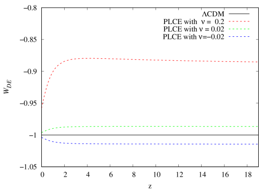
Figure 1: Evolutions of the equation-of-state parameter $w_{DE}$ in $\Lambda$CDM and PLCE models.

Because the PLCE model goes back to $\Lambda$CDM when $\nu=0$, we choose $\nu=\pm 0.02$ to compare the differences between the two models. We also take a larger value of $\nu=0.2$ to check the sensitivity of $\nu$. The results in Fig. 1 show that $w_{DE}$ does not overlap or cross -1 in any non-zero value of $\nu$. In addition, it maintains its value in the early universe, and only trends to -1 for $z<2$.

Figure 2: CMB power spectra of the TT mode in $\Lambda$CDM and PLCE models along with the Planck 2018 data.

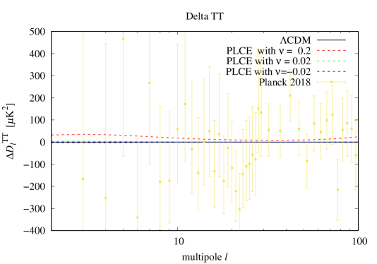
Figure 3: The change $\Delta D_{\ell}^{TT}$ of the TT mode of CMB power spectra between PLCE and $\Lambda$CDM, where the legend is the same as Fig. 1.

In Fig. 2, we display the CMB power spectra in the $\Lambda$CDM and PLCE models along with the data from Planck 2018. Since the TT spectra of PLCE and $\Lambda$CDM are almost identical to the data from Planck 2018 for the high values of the multipole $l$, we focus on the differences between the two models and the data when $l<100$ as depicted in Fig. 3. The TT power spectrum in the PLCE model for $\nu>0$ is larger than that of $\Lambda$CDM when $l<100$ with the error in the allowable range of the observational data.

For the TE mode, the spectra in PLCE for the different parameters $\nu$ are always close to that in $\Lambda$CDM as well as the observational data of Planck 2018, as shown in Fig. 4. However, when we carefully compare the differences between the results in PLCE and $\Lambda$CDM in Fig. 5, we notice that those of PLCE are closer to the Planck 2018 data, comparing to that in $\Lambda$CDM.

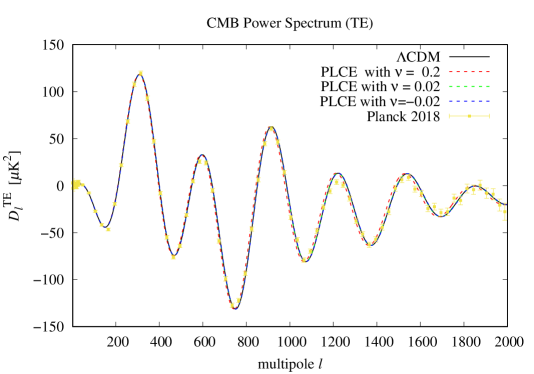
Figure 4: CMB TE power spectra in the $\Lambda$CDM and PLCE models along with the Planck 2018 data.

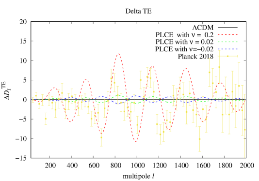
Figure 5: The change $\Delta D_{\ell}^{TE}$ of the TT mode of CMB power spectra between PLCE and $\Lambda$CDM, where the legend is the same as Fig. 4.

III.2 Tsallis Entropy Cosmological Evolution Model

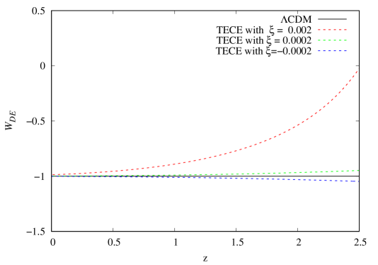
Figure 6: Evolutions of the equation-of-state parameter $w_{DE}$ in $\Lambda$CDM and TECE models.

Eq. (7) of TECE becomes the one in $\Lambda$CDM when $\delta=\tilde{\alpha}=1$. In our study, we only focus on the effects when $\delta\neq 1$ so we set $\tilde{\alpha}=1$ and $\delta=1+\xi$. In Fig. 6, we find that the equation of state, $w_{DE}$, behaves differently for different values of $\xi$. In particular, it is larger (smaller) than -1 when $\xi$ is larger (smaller) than zero without crossing -1 in anytime.

In Figs. 7 and  8, we see that the TT Power spectra of TECE and $\Lambda$CDM have a large difference in the large scale structure. Note that there is a significant discrepancy between $\Lambda$CDM and the data at $l\sim 20-27$. However, the spectrum of TECE for $\xi$=0.002 and $l\sim 20-27$ is below that in $\Lambda$CDM, and closer to the observational data of Planck 2018. The shifts of the TE mode between PLCE and $\Lambda$CDM are shown in Figs. 9 and 10.

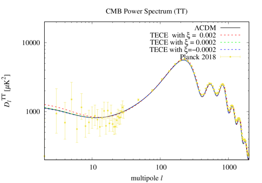
Figure 7: Legend is the same as Fig. 2 but in the TECE model with a set of $\xi$.

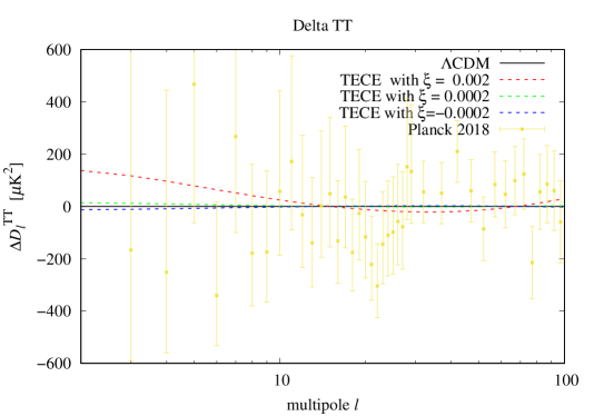
Figure 8: Legend is the same as Fig. 3 but in the TECE model with a set of $\xi$.

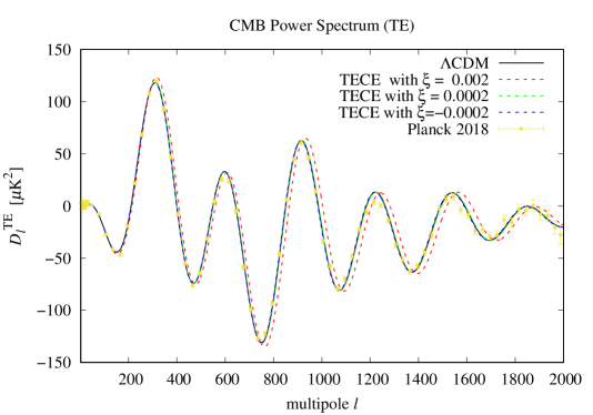
Figure 9: Legend is the same as Fig. 4 but in the TECE model with a set of $\xi$.

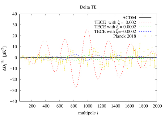
Figure 10: Legend is the same as Fig. 5 but in the TECE model with a set of $\xi$.

III.3 Global Fits

We use the modified ${\bf CAMB}$ and CosmoMC program Lewis:2002ah to do the global cosmological fits for the PLCE and TECE models from the observational data with the MCMC method. The dataset includes those of the CMB temperature fluctuation from Planck 2015 with TT, TE, EE, low-$l$ polarization and CMB lensing from SMICA Adam:2015wua ; Aghanim:2015xee ; Ade:2015zua , the weak lensing (WL) data from CFHTLenS  Heymans:2013fya , and the BAO data from 6dF Galaxy Survey Beutler:2011hx and BOSS Anderson:2013zyy . In particular, we include 35 points for the $H(z)$ measurements in our fits, which are listed in Table 1. The $\chi^{2}$ fit is given by

$${\chi^{2}}={\chi^{2}_{CMB}}+{\chi^{2}_{WL}}+{\chi^{2}_{BAO}}+{\chi^{2}_{H(z)}},$$ (13)

with

$$\chi^{2}_{c}=\sum_{i=1}^{n}\frac{(T_{c}(z_{i})-O_{c}(z_{i}))^{2}}{E^{i}_{c}}\,,$$ (14)

where the subscript of “$c$” denotes the category of the data, $n$ represents the number of the dataset, $T_{c}$ is the prediction from CAMB, and $O_{c}$ ($E_{c}$) corresponds to the observational value (covariance). The priors of the various cosmological parameters are given in Table 2.

Table 1: $H(z)$ data points

	$z$	$H(z)$	Ref.		$z$	$H(z)$	Ref.		$z$	$H(z)$	Ref.
1	0.07	69.0$\pm$19.6	Zhang:2012mp	13	0.4	95.0$\pm$17.0	Simon:2004tf	25	0.9	117.0$\pm$23.0	Simon:2004tf
2	0.09	69.0$\pm$12.0	Jimenez:2003iv	14	0.4004	77.0$\pm$10.2	Moresco:2016mzx	26	1.037	154.0$\pm$20.0	Moresco:2012jh
3	0.12	68.6$\pm$26.2	Zhang:2012mp	15	0.4247	87.1$\pm$11.2	Moresco:2016mzx	27	1.3	168.0$\pm$17.0	Simon:2004tf
4	0.17	83.0$\pm$8.0	Simon:2004tf	16	0.4497	92.8$\pm$12.9	Moresco:2016mzx	28	1.363	160.0$\pm$33.6	Moresco:2015cya
5	0.179	75.0$\pm$4.0	Moresco:2012jh	17	0.4783	80.9$\pm$9.0	Moresco:2016mzx	29	1.43	177.0$\pm$18.0	Simon:2004tf
6	0.199	75.0$\pm$5.0	Moresco:2012jh	18	0.48	97.0$\pm$62.0	Stern:2009ep	30	1.53	140.0$\pm$14.0	Simon:2004tf
7	0.2	72.9$\pm$29.6	Zhang:2012mp	19	0.57	92.4$\pm$4.5	Reid:2012sw	31	1.75	202.0$\pm$40.0	Simon:2004tf
8	0.27	77.0$\pm$14.0	Simon:2004tf	20	0.5929	104.0$\pm$13.0	Moresco:2012jh	32	1.965	186.5$\pm$50.4	Moresco:2015cya
9	0.24	79.69$\pm$2.65	Gaztanaga:2008xz	21	0.6797	92.0$\pm$8.0	Moresco:2012jh	33	2.3	224$\pm$8	Busca:2012bu
10	0.28	88.8$\pm$36.6	Zhang:2012mp	22	0.7812	105.0$\pm$12.0	Moresco:2012jh	34	2.34	222$\pm$7	Hu:2014vua
11	0.352	83.0$\pm$14.0	Moresco:2012jh	23	0.8754	125.0$\pm$17.0	Moresco:2012jh	35	2.36	226$\pm$8	Font-Ribera:2013wce
12	0.3802	83.0$\pm$13.5	Moresco:2016mzx	24	0.88	90.0$\pm$40.0	Stern:2009ep

Table 2: Priors for cosmological parameters in the PLCE and TECE models.

Parameter	Prior
PLCE Model parameter $\nu$	$-0.025\leq\nu\leq 1.0$
TECE Model parameter $\xi$	$-0.01\leq\xi\leq 0.02$
Baryon density	$0.5\leq 100\Omega_{b}h^{2}\leq 10$
CDM density	$0.1\leq 100\Omega_{c}h^{2}\leq 99$
Optical depth	$0.01\leq\tau\leq 0.8$
Neutrino mass sum	$0\leq\Sigma m_{\nu}\leq 2$ eV
$\frac{\mathrm{Sound\ horizon}}{\mathrm{Angular\ diameter\ distance}}$	$0.5\leq 100\theta_{MC}\leq 10$
Scalar power spectrum amplitude	$2\leq\ln\left(10^{10}A_{s}\right)\leq 4$
Spectral index	$0.8\leq n_{s}\leq 1.2$

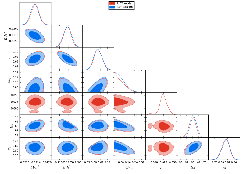
Figure 11: One and two-dimensional distributions of $\Omega_{b}h^{2}$, $\Omega_{c}h^{2}$, $\sum m_{\nu}$, $\nu$, $H_{0}$, and $\sigma_{8}$ in the PLCE and $\Lambda$CDM models, where the contour lines represent 68$\%$  and 95$\%$  C.L., respectively.

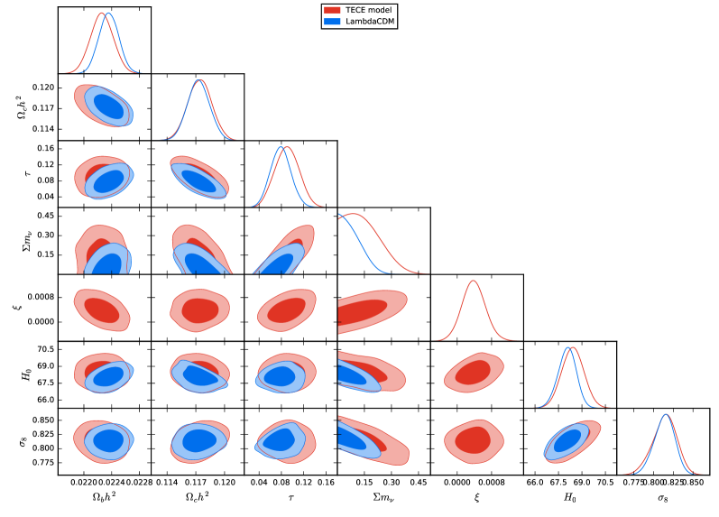
Figure 12: Legend is the same as Fig. 11 but for the TECE and $\Lambda$CDM models.

Table 3: Fitting results for the PLCE and $\Lambda$CDM models, where the limits are given at 68$\%$ and 95$\%$ C.L., respectively

Parameter	PLCE (68% C.L.)	PLCE (95% C.L.)	$\Lambda$CDM (68% C.L.)	$\Lambda$CDM (95% C.L.)
$\Omega_{b}h^{2}$	$0.02237\pm 0.00014$	$0.02237\pm 0.00027$	$0.02235\pm 0.00014$	$0.02235^{+0.00028}_{-0.00027}$
$\Omega_{c}h^{2}$	$0.1172^{+0.0012}_{-0.0011}$	$0.1172^{+0.0022}_{-0.0023}$	$0.1173\pm 0.0012$	$0.1173\pm 0.0023$
$100\theta_{MC}$	$1.04101\pm 0.00030$	$1.04101\pm 0.00059$	$1.04100\pm 0.00029$	$1.04100^{+0.00057}_{-0.00058}$
$\tau$	$0.079^{+0.017}_{-0.019}$	$0.079^{+0.036}_{-0.034}$	$0.078\pm 0.018$	$0.078^{+0.035}_{-0.034}$
$\Sigma m_{\nu}$/eV	$<0.0982$	$<0.183$	$<0.100$	$<0.195$
$\nu$	$0.0240^{+0.0110}_{-0.0085}$	$0.024^{+0.022}_{-0.033}$	$-$	$-$
${\rm{ln}}(10^{10}A_{s})$	$3.086^{+0.031}_{-0.035}$	$3.086^{+0.068}_{-0.063}$	$3.083\pm 0.033$	$3.083^{+0.066}_{-0.064}$
$H_{0}$	$67.96\pm 0.56$	$68.0\pm 1.1$	$68.14\pm 0.55$	$68.1\pm 1.1$
$\sigma_{8}$	$0.814^{+0.013}_{-0.011}$	$0.814^{+0.023}_{-0.026}$	$0.815^{+0.013}_{-0.011}$	$0.815^{+0.023}_{-0.025}$
$\chi^{2}_{best-fit}$	3017.12		3018.32

Table 4: Fitting results for the TECE and $\Lambda$CDM models, where the limits are given at 68$\%$ and 95$\%$ C.L., respectively

Parameter	TECE (68% C.L.)	TECE (95% C.L.)	$\Lambda$CDM (68% C.L.)	$\Lambda$CDM (95% C.L.)
$\Omega_{b}h^{2}$	$0.02226\pm 0.00016$	$0.02226^{+0.00033}_{-0.00032}$	$0.02236\pm 0.00014$	$0.02236^{+0.00028}_{-0.00027}$
$\Omega_{c}h^{2}$	$0.1174\pm 0.0013$	$0.1174\pm 0.0025$	$0.1173\pm 0.0012$	$0.1173\pm 0.0023$
$100\theta_{MC}$	$1.04125\pm 0.00036$	$1.04125^{+0.00073}_{-0.00069}$	$1.04099\pm 0.00031$	$1.04099^{+0.00062}_{-0.00060}$
$\tau$	$0.090\pm 0.021$	$0.090\pm 0.042$	$0.079\pm 0.018$	$0.079^{+0.037}_{-0.035}$
$\Sigma m_{\nu}$/eV	$<0.186$	$<0.317$	$<0.107$	$<0.195$
$\xi$	$0.00038\pm 0.00027$	$0.00038^{+0.00055}_{-0.00053}$	$-$	$-$
${\rm{ln}}(10^{10}A_{s})$	$3.103\pm 0.039$	$3.103\pm 0.076$	$3.085\pm 0.034$	$3.085^{+0.068}_{-0.065}$
$H_{0}$	$68.42\pm 0.71$	$68.4\pm 1.4$	$68.05^{+0.60}_{-0.54}$	$68.1^{+1.1}_{-1.2}$
$\sigma_{8}$	$0.814^{+0.017}_{-0.014}$	$0.814^{+0.028}_{-0.032}$	$0.814^{+0.014}_{-0.012}$	$0.814^{+0.024}_{-0.027}$
$\chi^{2}_{best-fit}$	3018.96		3019.28

In Fig. 11, we present our fitting results of PLCE (red) and $\Lambda$CDM (blue). Although the PLCE model has been discussed in the literature, it is the first time to illustrate its numerical cosmological effects. In particular, we find that $\nu$ = $(0.0240^{+0.0110}_{-0.0085})$ in 68$\%$ C.L., which shows that PLCE and $\Lambda$CDM can be clearly distinguished. It is interesting to note that the value of $\sigma_{8}$=$0.814^{+0.023}_{-0.026}$ (95$\%$ C.L.) in PLCE is smaller than that of $0.815^{+0.023}_{-0.025}$ (95$\%$ C.L.) in $\Lambda$CDM. As shown in Table 3, the best fitted $\chi^{2}$ value in PLCE is 3017.12, which is also smaller than 3018.32 in $\Lambda$CDM. Although the cosmological observables for the best $\chi^{2}$ fit in PLCE do not significantly deviate from those in $\Lambda$CDM, it indicates that the PLCE model is closer to the observational data than $\Lambda$CDM.

Similarly, we show our results for TECE (red) and $\Lambda$CDM (blue) in Fig. 12. Explicitly, we get that $\xi$ = $(3.8\pm{2.7})\times 10^{-4}$ in 68$\%$ C.L. In addition, the TECE model can relax the limit of the total mass of the active neutrinos. In particular, we have that $\Sigma m_{\nu}$ $<0.317$ eV, comparing to $\Sigma m_{\nu}$ $<0.195$ eV in $\Lambda$CDM at 95$\%$ C.L. In addition, the value of $H_{0}$ in TECE equals to $68.42\pm{0.71}$ $(68.4\pm{1.4})$, which is larger than $68.05^{+0.60}_{-0.54}$ $(68.1^{+1.1}_{-1.2})$ in $\Lambda$CDM with 68$\%$ (95$\%$) C.L.

As shown in Table 4, the best fitted $\chi^{2}$ value in the TECE model is 3018.96, which is smaller than 3019.28 in $\Lambda$CDM model. Although the difference between the value of $\chi^{2}$ in TECE and $\Lambda$CDM is not significant, it still implies that the TECE model can not be ignored. Clearly, more considerations and discussions are needed in the future.

IV Conclusions

We have calculated the cosmological evolutions of $\rho_{DE}$ and $w_{DE}$ in the PLCE and TECE models. We have found that the EoS of dark energy in PLCE (TECE) does not cross -1. We have shown that the CMB TE power spectrum of the PLCE model with a positive $\nu$ is closer to the Planck 2018 data than that in $\Lambda$CDM, while the CMB TT spectrum in the TECE model has smaller values around $l\sim 20-27$, which are lower than that in $\Lambda$CDM, but close to the data of Planck 2018. By using the Newton method in the global fitting, we have obtained the first numerical result in the PLCE model with $\nu=0.0240^{+0.0110}_{-0.0085}$ in 68$\%$ C.L., which can be distinguished well with $\Lambda$CDM. Our Fitting results indicate that the PLCE model gives a smaller value of $\sigma_{8}$ with a better $\chi^{2}$ value than $\Lambda$CDM. In the TECE model, we have gotten that $\xi=(3.8\pm 2.7)^{-4}$ and $\Sigma m_{\nu}$ $<0.186$ eV in 68$\%$ C.L., while $H_{0}$ is closer to 70. The best fitted value of $\chi^{2}$ is 3018.96 in the TECE model, which is smaller than 3019.28 in $\Lambda$CDM. These results have demonstrated that the TECE model deserves more attention and research in the future.

- (1) L. Amendola and S. Tsujikawa, Dark Energy : Theory and Observations, (Cambridge Univer- sity Press, 2015).
- (2) S. Weinberg, Rev. Mod. Phys. 61, 1 (1989).
- (3) S. Weinberg, Gravitation and Cosmology, (Wiley and Sons, New York, 1972).
- (4) N. Arkani-Hamed, L. J. Hall, C. F. Kolda and H. Murayama, Phys. Rev. Lett. 85, 4434 (2000).
- (5) P. J. E. Peebles and B. Ratra, Rev. Mod. Phys. 75, 559 (2003).
- (6) E. J. Copeland, M. Sami and S. Tsujikawa, Int. J. Mod. Phys. D 15, 1753 (2006).
- (7) T. Jacobson, Phys. Rev. Lett. 75, 1260 (1995).
- (8) R. G. Cai and S. P. Kim, JHEP 0502, 050 (2005).
- (9) M. Akbar and R. G. Cai, Phys. Lett. B 635, 7 (2006)
- (10) M. Akbar and R. G. Cai, Phys. Rev. D 75, 084003 (2007)
- (11) M. Jamil, E. N. Saridakis and M. R. Setare, Phys. Rev. D 81, 023007 (2010)
- (12) Z. Y. Fan and H. Lu, Phys. Rev. D 91, no. 6, 064009 (2015)
- (13) Y. Gim, W. Kim and S. H. Yi, JHEP 1407, 002 (2014)
- (14) S. Das, S. Shankaranarayanan and S. Sur, Phys. Rev. D 77, 064013 (2008).
- (15) C. Tsallis, J. Statist. Phys. 52, 479 (1988).
- (16) M. L. Lyra and C. Tsallis, Phys. Rev. Lett. 80, 53 (1998).
- (17) G. Wilk and Z. Wlodarczyk, Phys. Rev. Lett. 84, 2770 (2000).
- (18) D. A. Easson, P. H. Frampton and G. F. Smoot, Phys. Lett. B 696, 273 (2011).
- (19) N. Komatsu and S. Kimura, Phys. Rev. D 88, 083534 (2013).
- (20) E. M. C. Abreu et al., Physica A 441, 141 (2016); S. Ghaffari et al., Eur. Phys. J. C 78, 706 (2018); M. A. Zadeh, A. Sheykhi, H. Moradpour and K. Bamba, Eur. Phys. J. C 78, 940 (2018); E. N. Saridakis, K. Bamba, R. Myrzakulov and F. K. Anagnostopoulos, JCAP 1812, 012 (2018); M. Tavayef, A. Sheykhi, K. Bamba and H. Moradpour, Phys. Lett. B 781, 195 (2018).
- (21) E. M. Barboza et al., Physica A 436, 301 (2015).
- (22) M. Abdollahi Zadeh, A. Sheykhi and H. Moradpour, Mod. Phys. Lett. A 34, 1950086 (2019).
- (23) S. Nojiri, S. D. Odintsov and E. N. Saridakis, Eur. Phys. J. C 79, no. 3, 242 (2019).
- (24) C. Tsallis and L. J. L. Cirto, Eur. Phys. J. C 73, 2487 (2013).
- (25) K. Bamba, S. Capozziello, S. Nojiri and S. D. Odintsov, Astrophys. Space Sci. 342, 155 (2012).
- (26) A. Lymperis and E. N. Saridakis, Eur. Phys. J. C 78, 993 (2018).
- (27) W. H. Press et al., Numerical Recipes 3rd Edition: The Art of Scientific Computing, (Cambridge University Press, 2007).
- (28) A. Lewis and S. Bridle, Phys. Rev. D 66, 103511 (2002).
- (29) C. Zhang, H. Zhang, S. Yuan, T. J. Zhang and Y. C. Sun, Res. Astron. Astrophys. 14, 1221 (2014).
- (30) R. Jimenez, L. Verde, T. Treu and D. Stern, Astrophys. J. 593, 622 (2003).
- (31) J. Simon, L. Verde and R. Jimenez, Phys. Rev. D 71, 123001 (2005).
- (32) M. Moresco et al., JCAP 1208, 006 (2012).
- (33) E. Gaztanaga, A. Cabre and L. Hui, Mon. Not. Roy. Astron. Soc. 399, 1663 (2009).
- (34) M. Moresco et al., JCAP 1605, 014 (2016).
- (35) D. Stern, R. Jimenez, L. Verde, M. Kamionkowski and S. A. Stanford, JCAP 1002, 008 (2010).
- (36) B. A. Reid et al., Mon. Not. Roy. Astron. Soc. 426, 2719 (2012).
- (37) M. Moresco, Mon. Not. Roy. Astron. Soc. 450, L16 (2015).
- (38) N. G. Busca et al., Astron. Astrophys. 552, A96 (2013).
- (39) Y. Hu, M. Li and Z. Zhang, arXiv:1406.7695 [astro-ph.CO].
- (40) A. Font-Ribera et al. [BOSS Collaboration], JCAP 1405, 027 (2014).
- (41) R. Adam et al. [Planck Collaboration], Astron. Astrophys. 594, A10 (2016).
- (42) N. Aghanim et al. [Planck Collaboration], Astron. Astrophys. 594, A11 (2016).
- (43) P. A. R. Ade et al. [Planck Collaboration], Astron. Astrophys. 594, A15 (2016).
- (44) C. Heymans et al., Mon. Not. Roy. Astron. Soc. 432, 2433 (2013).
- (45) F. Beutler et al., Mon. Not. Roy. Astron. Soc. 416, 3017 (2011).
- (46) L. Anderson et al. [BOSS Collaboration], Mon. Not. Roy. Astron. Soc. 441, 24 (2014).