Including higher order multipoles in gravitational-wave models for precessing binary black holes

Abstract

Estimates of the source parameters of gravitational-wave (GW) events produced by compact binary mergers rely on theoretical models for the GW signal. We present the first frequency-domain model for inspiral, merger and ringdown of the GW signal from precessing binary-black-hole systems that also includes multipoles beyond the leading-order quadrupole. Our model, PhenomPv3HM, is a combination of the higher-multipole non-precessing model PhenomHM and the spin-precessing model PhenomPv3 that includes two-spin precession via a dynamical rotation of the GW multipoles. We validate the new model by comparing to a large set of precessing numerical-relativity simulations and find excellent agreement across the majority of the parameter space they cover. For mass ratios $<5$ the mismatch improves, on average, from $\sim 6\%$ to $\sim 2\%$ compared to PhenomPv3 when we include higher multipoles in the model. However, we find mismatches $\sim 8\%$ for a mass-ratio $6$ and highly spinning simulation. We quantify the statistical uncertainty in the recovery of binary parameters by applying standard Bayesian parameter estimation methods to simulated signals. We find that, while the primary black hole spin parameters should be measurable even at moderate signal-to-noise ratios (SNRs) $\sim 30$, the secondary spin requires much larger SNRs $\sim 200$. We also quantify the systematic uncertainty expected by recovering our simulated signals with different waveform models in which various physical effects, such as the inclusion of higher modes and/or precession, are omitted and find that even at the low SNR case ($\sim 17$) the recovered parameters can be biased. Finally, as a first application of the new model we have analysed the binary black hole event GW170729. We find larger values for the primary black hole mass of $58.25^{+11.73}_{-12.53}\,M_{\odot}$ (90% credible interval). The lower limit ($\sim 46\,M_{\odot}$) is comparable to the proposed maximum black hole mass predicted by different stellar evolution models due to the pulsation pair-instability supernova (PPISN) mechanism. If we assume that the primary Black Hole (BH) in GW170729 formed through a PPISN then out of the four PPISN models we considered only the model of  Woosley (2017) is consistent with our mass measurements at the 90% level.

I Introduction

The second generation Gravitational Wave (GW) detectors — Advanced LIGO Aasi et al. (2015) and Virgo Acernese et al. (2015) — have so far published observations of 11 compact binary mergers from the first two observing runs Abbott et al. (2018a), including one binary neutron star merger that was also observed across the electromagnetic spectrum Abbott et al. (2017). The third observing run is currently underway, with further sensitivity improvements planned in the coming years Abbott et al. (2018b). GW observations have already begun to constrain models of the formation and rates of stellar mass compact binary mergers Abbott et al. (2018c), and to make strong-field tests of the general theory of relativity Abbott et al. (2019).

Models for the GW signal, parametrized in terms of the properties of the system (such as masses, spins, and orientation), are compared with detector data to infer the source properties of GW events. The GW signal is commonly expressed in a multipole expansion where we denote terms beyond the leading order quadrupole contribution as “higher order multipoles”. These higher order multipoles are typically much weaker than the dominant quadrupolar multipole, but grow in relative strength for systems that are more asymmetric in mass. Past studies have shown that for events where the signal contains measurable power in the higher multipoles, parameter estimates can be biassed when using only a dominant-multipole model. Conversely, it is also true that for some systems we are able to measure the source parameters more accurately using a higher multipole model  Graff et al. (2015); London et al. (2018); Chatziioannou et al. (2019); Kalaghatgi et al. (2019); Calderón Bustillo et al. (2018); Shaik et al. (2019).

Another important physical effect is spin precession, where couplings between the orbital and spin angular momenta can cause the orbital plane to precess and thus cause modulations of the observed GW Apostolatos et al. (1994); Kidder (1995). In terms of the GW multipoles, precession mixes together different orders ($m$-multipoles) of the same degree ($\ell$-multipoles), complicating a simple description of the waveform Schmidt et al. (2011a); Boyle et al. (2011); O’Shaughnessy et al. (2012); Schmidt et al. (2012); Pekowsky et al. (2013); Boyle et al. (2014); O’Shaughnessy et al. (2011); Fairhurst et al. (2019). By not taking into account precession and higher order multipoles in our waveform models we may not be able to confidently detect and accurately characterize signals where these effects are important Capano et al. (2014); Varma and Ajith (2017); Calderón Bustillo et al. (2018); Harry et al. (2016, 2018); Calderón Bustillo et al. (2016). These events are also likely to be very interesting astrophysically, providing valuable information about Binary Black Hole (BBH) formation mechanisms and hence are events with high scientific gain that we wish to model and measure accurately.

The field of waveform modeling has seen sustained development over almost two decades and is currently thriving, with improvements to current and development of novel methods allowing for more accurate and efficient models to be applied in data analysis pipelines  Buonanno and Damour (1999); Pan et al. (2014a); Buonanno and Damour (2000); Pan et al. (2011); Taracchini et al. (2014); Blanchet (2014); Hannam et al. (2014); Ajith et al. (2007a); Santamaría et al. (2010); Khan et al. (2016); London et al. (2018); Cotesta et al. (2018); Bohé et al. (2017); Babak et al. (2017); Blackman et al. (2017a); Nagar et al. (2018); Mehta et al. (2019); Varma et al. (2019a); Williams et al. (2019); Setyawati et al. (2019); Khan et al. (2019); Lundgren and O’Shaughnessy (2014); Doctor et al. (2017); Blackman et al. (2017b); Varma et al. (2019b). In this work we take a step towards including as many important physical effects as possible in waveform models, by constructing the most physically complete phenomenological model to date. We present a frequency-domain model for the GW signal from the inspiral, merger and ringdown of a BBH system. The BHs are allowed to precess and we also model the contribution to the GW signal from higher order multipoles. This combines the progress made in two earlier models: a precessing-binary model that includes accurate two-spin precession effects during the inspiral Chatziioannou et al. (2017a, b) (PhenomPv3 Khan et al. (2019)), and an approximate higher-multipole aligned-spin model (PhenomHM London et al. (2018)).

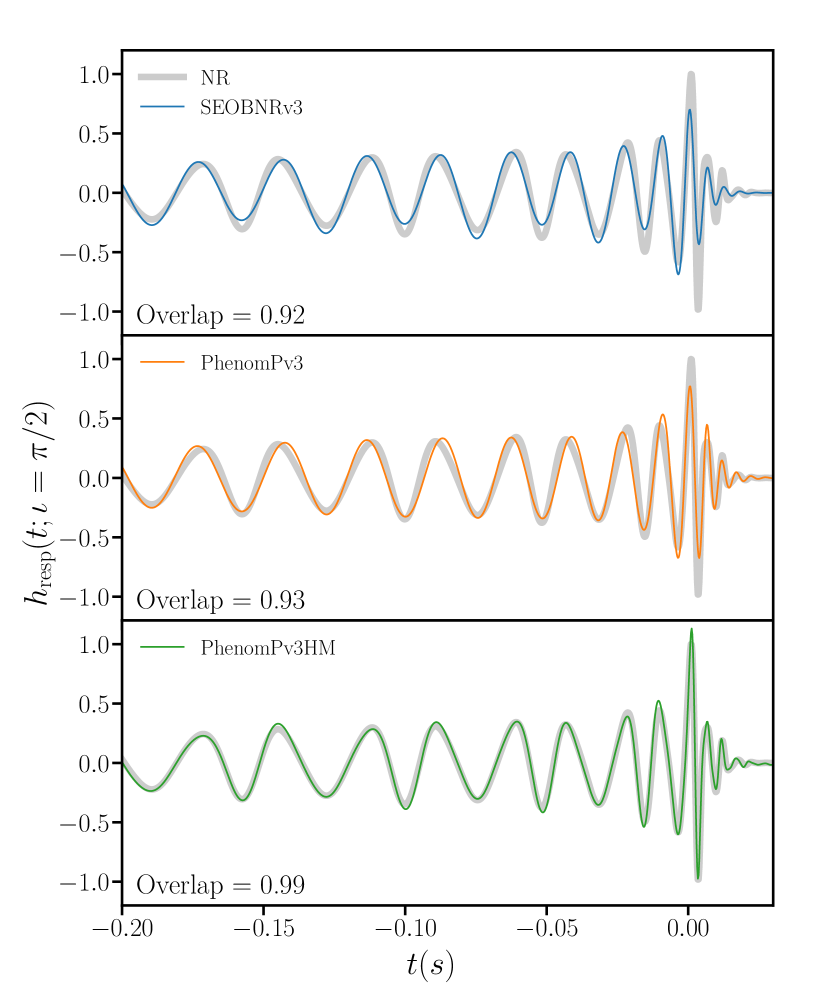
Figure 1: Comparison of the detector response strain $h(t)$ viewed at an inclination angle of $\pi/2$. Solid grey: NR simulation (SXS:BBH:0058). A mass-ratio $q\equiv m_{1}/m_{2}=5$, precessing BBH simulation with a dimensionless-spin magnitude of $\chi_{1}=0.5$ generated with a total mass of $80M_{\odot}$. The NR signal contains all the $\ell,m$ modes up to and including $\ell=4$. Top panel, blue: Precessing model SEOBNRv3 Pan et al. (2014b), with the $((2,\pm 2),(2,\pm 1))$ modes in the co-precessing frame. Middle panel, orange: Precessing model PhenomPv3 Khan et al. (2019) with only the $2,\pm 2$ modes in the co-precessing frame. Bottom panel, green: Precessing model presented here, PhenomPv3HM, with the $(\ell,|m|)=((2,2),(2,1),(3,3),(3,2),(4,4),(4,3))$ modes in the co-precessing frame. The orientation-averaged mismatch $1-\overline{\mathcal{M}}$ (see Sec. III.1) is $8\,\%$ for the top panel, $7\,\%$ for the middle and $1\,\%$ for the bottom. We only plot the last $\sim$7 GW cycles for clarity but the behaviour is qualitatively the same throughout the 29-orbit inspiral ($\sim$60 GW cycles).

Figure 1 demonstrates the improved accuracy that is achievable by our new model, PhenomPv3HM, compared to other existing models that include the effect of spin precession, but not higher order multipoles. We compare the observed GW signal predicted by our new model against a high-mass-ratio, precessing NR simulation (thick grey line). We plot the GW signal observed at an inclination angle of $\pi/2$ rad to emphasise the effect of precession. We use all multipoles in the range $2\leq\ell\leq 4$ when computing the NR GW polarisations.

We compute the mismatch (defined in Section III.1) between three different precessing waveform models and the NR waveform, and average over all possible orientations. The top panel shows the optimal waveform (in blue) when we use SEOBNRv3 Babak et al. (2017) and the middle panel shows (in orange) the result when we use PhenomPv3. In this context the optimal waveform maximises the overlap over coalescence time, template phase and polarisation angle and the intrinsic parameters are fixed to the values from the NR simulation. As shown in Khan et al. (2019) SEOBNRv3 and PhenomPv3 have overlaps of $\sim 99\,\%$ and $\sim 98\,\%$ respectively to this NR waveform when only the $\ell=2$ multipoles are considered. When we include higher order multipoles in the NR waveform we find the overlap drops to only $\sim 92\,\%$ and $\sim 93\,\%$ respectively. This is an example where the exclusion of higher multipoles in template models can lead to unacceptable losses in signal-to-noise ratio (SNR). The bottom panel shows, in green, the best fitting PhenomPv3HM template. We find remarkable agreement, even through the inspiral, merger and ringdown stages. The overlap is now $99\,\%$ and the subtle modulation visible is accurately captured by our model. It is useful to point out here that, in PhenomPv3HM, the higher multipole and the precession elements of the model have not been calibrated to NR simulations, but when this is done we expect the accuracy to improve further.

The rest of the paper is organized as follows. In Sec. II we describe how our model is constructed. In Sec. III.1 we present results where we have compared our model against precessing NR simulations including higher order mutlipoles up to and including $\ell=4$ to demonstrate its accuracy across the parameter space where we have NR simulations. We have also performed a parameter estimation study to quantify the impact on parameter recovery when using a model that includes both higher multipoles and precession, the results of which are presented in section III.2.

Finally, in section III.3 we have analysed data for the GW170729 event, publicly available at the Gravitational Wave Open Science Center (GWOSC) Vallisneri et al. (2015), which has evidence for non-zero BH spin Abbott et al. (2018a) and unequal masses Chatziioannou et al. (2019).

II Method

Our method to build a model for the GW signal from precessing BBHs is based upon the novel ideas of Refs. Schmidt et al. (2011b); O’Shaughnessy et al. (2011); Boyle et al. (2011), where the GW from precessing binaries can be modelled as a dynamic rotation of non-precessing systems. In Refs. Hannam et al. (2014); Taracchini et al. (2014); Pan et al. (2014b) the authors used these ideas to build the first precessing Inspiral-Merger-Ringdown (IMR) models.

Our goal is to derive frequency-domain expressions for the GW polarisations $\tilde{h}_{+/\times}(f)$ in terms of the multipoles $\tilde{h}_{\ell m}(f)$. We start from the complex GW quantity, $h=h_{+}-ih_{\times}$, in the time-domain and decompose this into spin weight $-2$ spherical harmonics,

$$h(t,\vec{\lambda},\theta,\phi)=\sum_{\ell\geqslant 2}\sum_{-\ell\leqslant m\leqslant\ell}h_{\ell,m}(t,\vec{\lambda}){}_{-2}Y_{\ell,m}(\theta,\phi)\,.$$ (1)

This is a function of the time $t$, the intrinsic source parameters (masses and spin angular momenta of the bodies) denoted by $\vec{\lambda}$, and the polar angles $\theta$ and $\phi$ of a coordinate system whose $z-$axis is aligned with the total angular momentum $\vec{J}$ of the binary at some reference frequency. To approximate the precessing multipoles $h^{prec}_{\ell,m}(t)$ we perform a dynamic rotation of the non-precessing multipoles $h_{\ell,m}^{\begin{subarray}{c}non-\\ prec\end{subarray}}(t)$,

$$h^{prec}_{\ell,m}(t)=\sum_{-\ell\leqslant m^{\prime}\leqslant\ell}h^{\begin{subarray}{c}non-\\ prec\end{subarray}}_{\ell,m^{\prime}}(t)\,D^{\ell}_{m^{\prime},m}(\alpha(t),\beta(t),\epsilon(t))\,.$$ (2)

We define the Wigner D-matrix as $D^{\ell}_{m^{\prime},m}(\alpha,\beta,\epsilon)=e^{im\alpha}d^{\ell}_{m^{\prime},m}(-\beta)e^{-im^{\prime}\epsilon}$ and the Wigner d-matrix is given in Ref. Ajith et al. (2007b).

Next we transform to the frequency domain using the stationary phase approximation Droz et al. (1999) under the assumption that the precession angles modify the signal via a slowly varying amplitude, giving us an expression for the frequency-domain multipoles in terms of the co-precessing frame multipoles,

$$\tilde{h}^{prec}_{\ell,m}(f)=\sum\limits_{-\leqslant\ell<m^{\prime}\leqslant\ell}\tilde{h}^{\begin{subarray}{c}non-\\ prec\end{subarray}}_{\ell,m^{\prime}}(f)\,D^{\ell}_{m^{\prime},m}(\alpha,\beta,\epsilon)\,.$$ (3)

For brevity we omit the explicit dependence on frequency for the the precession angles $(\alpha,\beta,\epsilon)$ but they are evaluated at the stationary points $t(f)=2\pi f/m^{\prime}$  Santamaría et al. (2010).

The frequency-domain GW polarisations $\tilde{h}_{+/\times}(f)$ are defined as the Fourier transform (FT) of the real-valued GW polarisations $h_{+/\times}(t)$, which we write as,

$$\tilde{h}_{+}(f) = {\rm{FT}}\left[{\rm{Re}}(h(t))\right]=\frac{1}{2}\left(\tilde{h}(f)+\tilde{h}^{*}(-f)\right)\,,$$ (4)

$$\tilde{h}_{\times}(f) = {\rm{FT}}\left[{\rm{Im}}(h(t))\right]=\frac{i}{2}\left(\tilde{h}(f)-\tilde{h}^{*}(-f)\right)\,.$$ (5)

To arrive at the final expression for the frequency-domain GW polarisations we substitute Eq. (3) into Eqs. (4) and (5), assuming $f>0$ and symmetry through the orbital plane in the co-precessing frame, leading to,

$$\tilde{h}^{prec}_{+}(f) =\frac{1}{2}\sum_{\ell\geqslant 2}\sum_{m^{\prime}>0}\tilde{h}_{\ell,m^{\prime}}^{\begin{subarray}{c}non-\\ prec\end{subarray}}(f)\sum_{m=-\ell}^{\ell}\left(A^{\ell}_{m^{\prime},m}+(-1)^{\ell}A^{*\ell}_{-m^{\prime},m}\right)\,,$$ (6)

$$\tilde{h}^{prec}_{\times}(f) =-\frac{i}{2}\sum_{\ell\geqslant 2}\sum_{m^{\prime}>0}\tilde{h}_{\ell,m^{\prime}}^{\begin{subarray}{c}non-\\ prec\end{subarray}}(f)\sum_{m=-\ell}^{\ell}\left(A^{\ell}_{m^{\prime},m}-(-1)^{\ell}A^{*\ell}_{-m^{\prime},m}\right)\,.$$ (7)

To shorten the expression we define the auxillary matrix $A^{\ell}_{m^{\prime},m}\equiv{}_{-2}Y_{\ell,m}D^{\ell}_{m^{\prime},m}$ and omit the explicit angular dependence of ${}_{-2}Y_{\ell,m}$ and the precession angles in $D^{\ell}_{m^{\prime},m}$. The summation over $\ell$ and $m^{\prime}$ are over the modes included in the co-precessing frame. Here we use the PhenomHM model London et al. (2018), which contains the $(\ell,|m^{\prime}|)=((2,2),(2,1),(3,3),(3,2),(4,4),(4,3))$ modes.

Due to precession the properties of the remnant BH in the precessing system are different to those in the equivalent non-precessing system. We use the same prescription as described in Sec.III.C of Ref. Khan et al. (2019) to include the in-plane-spin contribution to the spin of the remnant BH. This modified final spin vector changes the ringdown spectrum of the aligned-spin multipoles.

Lastly, we note that the models for the three ingredients (the non-precessing model, the precession angles, and the BH remnant model) are independent in our construction, and can therefore each be updated when any of them are improved.

III Waveform assessment

III.1 Mismatch Computation

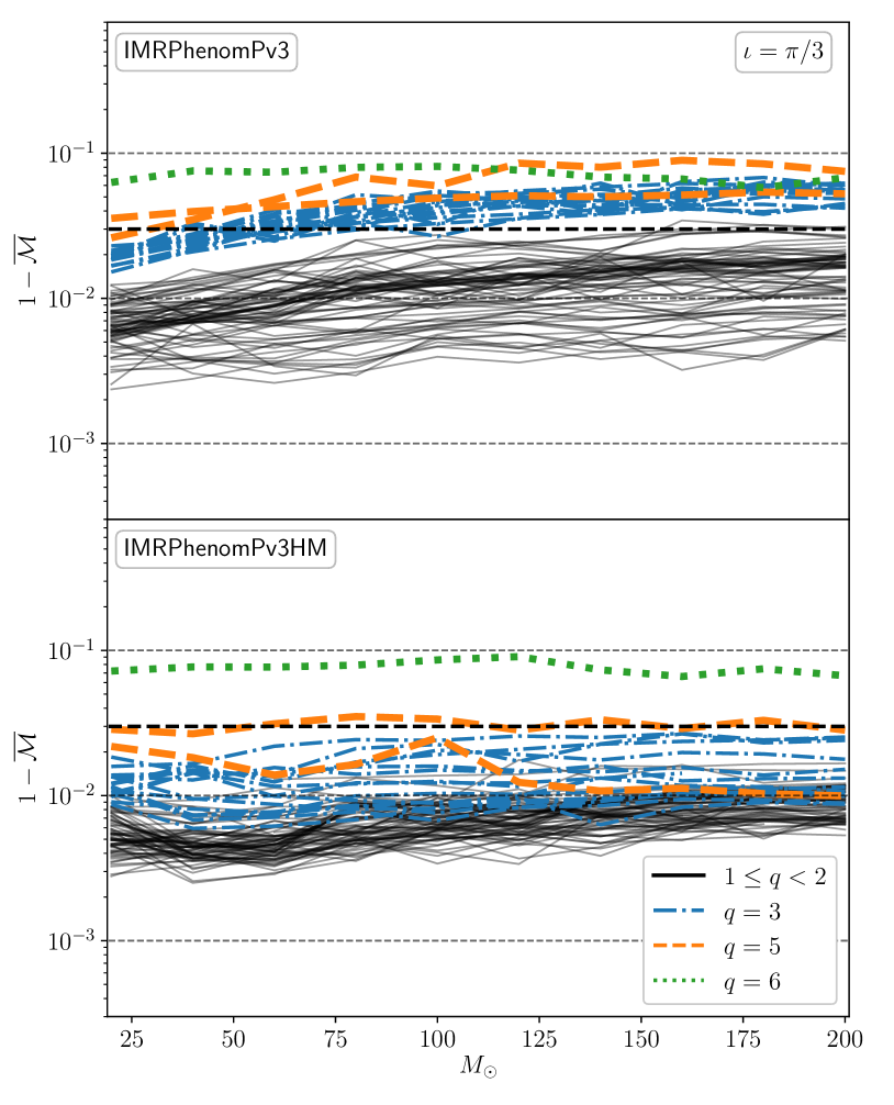
Figure 2: The results of the comparison between PhenomPv3 (top), PhenomPv3HM (bottom) and the precessing NR simulations from the public SXS catalogue. The figure shows the mismatch average over a reference phase and polarisation angle ($1-\overline{\mathcal{M}}$) as a function of the total mass for an inclination of $\iota=\pi/3$. The worst case is SXS:BBH:0165, a short ($\sim$6 orbits) signal with mass ratio 1:6 and high precession.

Waveform Model	PhenomPv3			PhenomPv3HM
Mass-Ratio ($\#$)	$0$	$\pi/3$	$\pi/2$	$0$	$\pi/3$	$\pi/2$
$1\leqslant q\leqslant 2$ (72)	$0.998^{0.999}_{0.993}$	$0.989^{0.996}_{0.977}$	$0.982^{0.993}_{0.967}$	$0.997^{0.999}_{0.993}$	$0.993^{0.996}_{0.986}$	$0.987^{0.992}_{0.972}$
$q=3$ (15)	$0.989^{0.999}_{0.974}$	$0.959^{0.967}_{0.950}$	$0.941^{0.946}_{0.933}$	$0.993^{0.997}_{0.985}$	$0.987^{0.993}_{0.975}$	$0.984^{0.989}_{0.974}$
$q=5$ (2)	$0.973^{0.978}_{0.968}$	$0.941^{0.951}_{0.931}$	$0.911^{0.925}_{0.897}$	$0.990^{0.990}_{0.989}$	$0.971^{0.975}_{0.966}$	$0.978^{0.989}_{0.968}$
$q=6$ (1)	$0.863$	$0.919$	$0.939$	$0.950$	$0.914$	$0.898$

Table 1: Match results from Sec. III.1. We quote the mean value of the match for each inclination angle considered ($\iota\in[0,\pi/3,\pi/2]$ rad) and averaged over all cases in the mass-ratio category for the $M_{tot}=100M_{\odot}$ case. The subscript and superscript are the minimum and maximum values of the match for the mass-ratio category considered.

The standard metric to assess the accuracy of GW signal models is to calculate the noise-weighted inner product between the template model and an accurate signal waveform. As our signal we use NR waveforms from the publicly available SXS catalogue Mroué et al. (2013); sxs ; Boyle et al. (2019) generated using the NR injection infrastructure in LALSuite Schmidt et al. (2017). From this catalogue we select the precessing configurations with the highest numerical resolution. This set contains 90 systems with $q\in[1,6]$, however, the majority of cases have $q\leqslant 3$. We have 2 cases at $q=5$ and one case at $q=6$. There are six cases that have at least one BH with a dimensionless spin magnitude $|\chi|>0.5$ whereas the majority of cases have $|\chi|\leqslant 0.5$ . For the exact list of NR configurations and specific details on how the mismatch calculations were performed we refer the reader to Ref. Khan et al. (2019) where we presented an identical analysis but restricted the signals to contain the $\ell=2$ multipoles.

Since PhenomPv3 is constructed from PhenomD it only has the $\ell=|m|=2$ modes in the co-precessing frame and therefore we expect this model to perform poorly when the contribution to the signal due to higher modes is not negligible. As PhenomPv3HM is constructed from PhenomHM and contains the $(\ell,|m|)=((2,2),(2,1),(3,3),(3,2),(4,4),(4,3))$ modes in the co-precessing frame we expect it to outperform PhenomPv3. In the NR signal we include multipoles with $\ell\in[2,4]$ to be consistent with the highest modeled $\ell$ mode in PhenomPv3HM.

We use the expected noise curve for Advanced LIGO operating at design sensitivity ali (a) with a low-frequency cutoff of $10{\rm{Hz}}$. Due to the presence of higher modes the orbital phase of the binary is no longer degenerate with the phase of the observed waveform, which means the standard method to analytically maximise over the template phase is not applicable. It is possible, however, to analytically maximise over the template polarisation using the skymax-SNR derived in Ref. Harry et al. (2016). In our match calculation we analytically maximise over the template polarisation and relative time shift and numerically optimise over the template orbital reference phase and frequency. Finally we average the match, weighted by the optimal SNR, over the signal orbital reference phase and polarisation angle. See Sec. III A in Ref. Khan et al. (2019) for details.

Figure 2 shows the orientation-averaged-mismatch Khan et al. (2019) as a function of the total mass of the binary for an inclination angle $\iota=\pi/3$. Here $\iota$ is the angle between the Newtonian orbital angular momentum and the line of sight at the start frequency of the NR waveform. The first row uses the dominant multipole-only model, PhenomPv3, and the second row uses the new higher multipole model, PhenomPv3HM, presented here. We clearly see that for $q\geqslant 3$ that it is important to include higher modes in the template model.

In Table 1 we summarise the results of our validation study by tabulating the results as the match (as opposed to mismatch as in Fig. 2) for each model according to mass ratio and inclination angle. Next to the mass-ratio range in parentheses is the number of NR cases in that mass-ratio category. Each entry in the table is calculated as follows: for the $M_{tot}=100M_{\odot}$ case we average the match over all cases in the mass-ratio category and write the minimum and maximum match as subscript and superscript respectively.

$1\leqslant q\leqslant 2$:

In this mass-ratio range both PhenomPv3 and PhenomPv3HM perform comparably, most likely due to the strength of higher multipoles scaling with mass ratio.

$q=3$:

Here we start to see the importance of the higher multipoles to accurately describe the NR signal. For $\iota=0$ PhenomPv3 has an average match of $0.989$. However, as the inclination angle increases, thus emphasising more of the higher multipole content of the signal, the average match drops to $0.941$ and can be as low as $0.933$. On the other hand, PhenomPv3HM is able to describe the NR data to an average accuracy of $0.984$ with a minimum value of $0.974$ for inclined systems.

$q=5$:

At this mass-ratio the loss in performance for PhenomPv3 is noticable even for low inclination values. At $\iota=0$ the average match is $0.973$ dropping to $0.911$ at $\iota=\pi/2$. The match for PhenomPv3HM at $\iota=0$ remains high at $0.99$, but reduces to $0.978$ at $\iota=\pi/2$. Note that we only have two NR simulations at $q=5$ and are thus unable to rigorously test the model at this and similar mass ratios.

$q=6$:

When comparing to this NR simulation we find both models perform substantially worse than the $q=5$ cases with even PhenomPv3 outperforming PhenomPv3HM with matches as low as $0.898$. We have verified that we obtain matches of $\sim 0.97$ when restricting the NR waveform to just the $\ell=2$ multipoles, consistent with our previous study Khan et al. (2019). We conclude that either our model is outside its range of validity or that this NR simulation is inaccurate for the higher multipoles, however, our results are robust against NR simulations of this configuration at multiple resolutions. This NR simulation, SXS:BBH:0165 is exceptional for a few reasons. First, it is a high mass-ratio system where higher multipoles are more important. Second, it is a strongly precessing system with primary $\chi_{1}=(0.74,0.19,-0.5)$ and secondary $\chi_{2}=(-0.19,0.,-0.23)$ spin vectors. Finally, it is also very short, only containing $\sim 6.5$ orbits. We encourage more NR simulations in this region by different NR codes to (i) cross check the results and (ii) populate this region with more data with which to test and refine future models.

We conclude from our study that PhenomPv3HM greatly improves the accuracy towards precessing BBHs for systems with mass-ratio up to 5:1. We expect to be able to greatly improve the accuracy and extend towards higher mass-ratio by further calibrating the higher order multipoles and precession effects to NR simulations.

III.2 Parameter Uncertainty

One of the main purposes of a waveform model is to estimate the source parameters of GW events. With models we can quantify the expected parameter uncertainty as a function of the parameter space  Vitale et al. (2017); Vitale and Evans (2017); Kumar et al. (2018); Ghosh et al. (2016); Pankow et al. (2017); Vitale et al. (2014); Farr et al. (2016); Pürrer et al. (2016); Stevenson et al. (2017); Vitale et al. (2017). Instead of a computationally intense systematic parameter estimation campaign we have chosen to focus on one configuration and study in detail the dependency of parameter recovery on SNR. We wish to study a system where both precession and higher modes are important and guided by previous studies Capano et al. (2014); Varma and Ajith (2017); Calderón Bustillo et al. (2017) we chose to study a double precessing spin, mass-ratio 3 BBH signal with a total mass of $150M_{\odot}$ in the detector frame. Starting at a frequency of $10$ Hz this system produces a waveform with about 20 GW cycles and merges at a frequency of about $120$ Hz. See Table 2 for specific injection values, where $(\theta_{JN},\phi)$ define the direction of propagation in the source frame, $(\alpha,\delta)$ are the right-ascension and declination of the source and $\psi$ is the polarisation angle.

We simulate this fiducial signal with PhenomPv3HM and recover its parameters using the parallel tempered MCMC algorithm implemented as LALInferenceMCMC in the publicly available LALInference software Veitch et al. (2015a) with PhenomPv3HM as the template model. We perform three separate, zero-noise, injections to investigate how our results depend on the injected SNR. Specifically we inject the signal at luminosity distances of 3000 Mpc, 1500 Mpc and 300 Mpc corresponding to a three-detector network SNR of 17, 35 and 176 respectively. We use the design sensitivity noise curves for the LIGO Hanford, LIGO Livingston and Virgo detectors ali (a).

We present our results by tabulating the median and 90% credible interval on binary parameters in Tab. 2 and source frame parameters in Tab. 3. We also plot the 90% credible interval as a function of the injected SNR for a few chosen parameters in Figs. 3, 4 and 5. In the high SNR limit the uncertainty on the parameters should decrease linearly wtih SNR i.e., as $1/\rho$ Vallisneri (2008), which is shown as a dashed black line in these figures.

In the following discussion we change our convention for the mass-ratio to $q\equiv m_{2}/m_{1}\in[0,1]$ and will abbreviate the width of the 90% credible interval of parameter $X$ at an SNR of $\rho$ as $C_{90\%}^{\rho}(X)$.

Parameter	Injection Value	$\rho=17.6$ $D_{L}=3000$	$\rho=35.2$ $D_{L}=1500$	$\rho=176$ $D_{L}=300$
$m^{\rm{det}}_{1}/M_{\odot}$	112.500	$102.98^{+13.38}_{-12.26}$	$107.71^{+7.96}_{-7.43}$	$112.38^{+1.73}_{-1.75}$
$m^{\rm{det}}_{2}/M_{\odot}$	37.500	$40.62^{+5.92}_{-5.29}$	$39.00^{+2.88}_{-2.66}$	$37.55^{+0.54}_{-0.52}$
$M_{\rm{total}}^{\rm{det}}/M_{\odot}$	150.000	$143.64^{+11.28}_{-9.74}$	$146.78^{+6.48}_{-5.94}$	$149.93^{+1.49}_{-1.46}$
$\mathcal{M}_{c}^{\rm{det}}/M_{\odot}$	54.940	$55.08^{+3.37}_{-3.20}$	$55.05^{+1.69}_{-1.69}$	$54.95^{+0.36}_{-0.34}$
$q$	0.333	$0.39^{+0.11}_{-0.08}$	$0.36^{+0.05}_{-0.04}$	$0.33^{+0.01}_{-0.01}$
$\theta_{1}$ / rad	1.052	$1.14^{+0.36}_{-0.37}$	$1.10^{+0.27}_{-0.19}$	$1.05^{+0.04}_{-0.04}$
$\theta_{2}$ / rad	2.090	$1.73^{+1.01}_{-1.21}$	$2.04^{+0.72}_{-1.09}$	$2.09^{+0.14}_{-0.12}$
$\Delta\phi_{12}$ / rad	1.571	$2.82^{+3.11}_{-2.49}$	$1.79^{+3.42}_{-1.35}$	$1.58^{+0.24}_{-0.24}$
$\theta_{JN}$ / rad	1.050	$1.62^{+0.60}_{-0.73}$	$1.21^{+0.92}_{-0.23}$	$1.05^{+0.03}_{-0.03}$
$\cos(\phi)$	1.000	$-0.04^{+1.03}_{-0.96}$	$0.46^{+0.54}_{-1.46}$	$1.00^{+0.00}_{-0.01}$
$\alpha$ / rad	1.047	$4.235^{+0.124}_{-3.213}$	$1.070^{+3.277}_{-0.036}$	$1.047^{+0.004}_{-0.004}$
$\delta$ / rad	1.047	$-1.020^{+2.098}_{-0.125}$	$1.025^{+0.037}_{-2.155}$	$1.047^{+0.004}_{-0.004}$
$\psi$ / rad	1.047	$1.52^{+0.66}_{-0.76}$	$1.28^{+0.80}_{-0.39}$	$1.05^{+0.04}_{-0.04}$
$\chi_{\rm{eff}}$	0.200	$0.204^{+0.129}_{-0.136}$	$0.201^{+0.070}_{-0.074}$	$0.200^{+0.016}_{-0.017}$
$\chi_{p}$	0.700	$0.681^{+0.186}_{-0.285}$	$0.705^{+0.098}_{-0.105}$	$0.699^{+0.020}_{-0.024}$
$|\chi_{1}|$	0.806	$0.77^{+0.15}_{-0.27}$	$0.80^{+0.07}_{-0.09}$	$0.81^{+0.02}_{-0.02}$
$|\chi_{2}|$	0.806	$0.45^{+0.47}_{-0.40}$	$0.59^{+0.35}_{-0.42}$	$0.80^{+0.13}_{-0.11}$
$D_{L}$ / Mpc	see heading	$3086.50^{+739.44}_{-571.98}$	$1465.76^{+177.84}_{-157.87}$	$300.12^{+7.14}_{-6.94}$

Table 2: Injection parameters and results from parameter estimation of simulated signals. We quote the median and 90% credible interval.

	$\rho$=17		$\rho$=34		$\rho$=176
Parameter	Inj.	Rec.	Inj.	Rec.	Inj.	Rec.
$m^{\rm{src}}_{1}/M_{\odot}$	74.56	$67.60^{+8.22}_{-8.35}$	87.789	$84.28^{+5.36}_{-5.24}$	105.724	$105.54^{+1.55}_{-1.58}$
$m^{\rm{src}}_{2}/M_{\odot}$	24.853	$26.60^{+3.95}_{-3.55}$	29.263	$30.48^{+2.47}_{-2.21}$	35.241	$35.27^{+0.51}_{-0.50}$
$M_{\rm{total}}^{\rm{src}}/M_{\odot}$	99.413	$94.35^{+6.64}_{-7.16}$	117.052	$114.82^{+3.97}_{-3.96}$	140.965	$140.80^{+1.28}_{-1.27}$
$M_{c}^{\rm{src}}/M_{\odot}$	36.412	$36.11^{+2.29}_{-2.34}$	42.872	$43.04^{+1.31}_{-1.28}$	51.631	$51.61^{+0.31}_{-0.30}$
$D_{L}/\rm{Mpc}$	3000	$3086.50^{+739.44}_{-571.98}$	1500	$1465.76^{+177.84}_{-157.87}$	300	$300.12^{+7.14}_{-6.94}$
$z$	0.509	$0.52^{+0.10}_{-0.08}$	0.281	$0.28^{+0.03}_{-0.03}$	0.064	$0.065^{+0.001}_{-0.001}$

Table 3: Source frame injection parameters and results from parameter estimation of simulated signals. We quote the median and 90% credible interval.

III.2.1 Masses

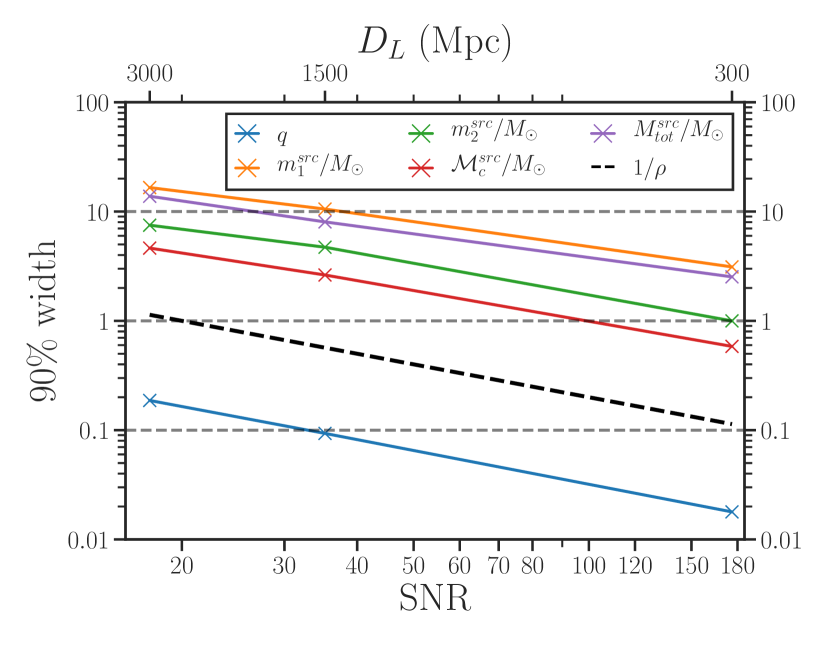
Figure 3: 90% credible intervals for the source frame mass parameters as a function of injected SNR

Figure 3 shows the source frame mass parameters; primary mass $m^{\rm{src}}_{1}$, secondary mass $m^{\rm{src}}_{2}$, chirp mass $\mathcal{M}_{c}^{\rm{src}}$, total mass $M_{\rm{total}}^{\rm{src}}$ and mass-ratio $q$. We find good scaling with respect to $1/\rho$ for all source frame mass parameters.

Table 3 shows the injection and recovered values. Even at the high total masses we consider here we find that the chirp mass is still the best measured parameter with $C_{90\%}^{17}(\mathcal{M}_{c}^{\rm{src}})=4.63M_{\odot}$ and $C_{90\%}^{176}(\mathcal{M}_{c}^{\rm{src}})=0.61M_{\odot}$. The total mass is the next best measured mass parameter with low and high SNR accuracies of $C_{90\%}^{17}(M_{\rm{total}}^{\rm{src}})=13.8M_{\odot}$ and $C_{90\%}^{176}(M_{\rm{total}}^{\rm{src}})=2.55M_{\odot}$ respectively. We find the primary mass can be measured to an accuracy of $C_{90\%}^{17}(m^{\rm{src}}_{1})=16.57M_{\odot}$ for low SNR and $C_{90\%}^{176}(m^{\rm{src}}_{1})=3.13M_{\odot}$ for high SNR. And for the secondary mass we find $C_{90\%}^{17}(m^{\rm{src}}_{2})=7.5M_{\odot}$ and $C_{90\%}^{176}(m^{\rm{src}}_{2})=1.01M_{\odot}$ for low and high SNR respectively. Finally, we are able to constrain the mass-ratio to $C_{90\%}^{17}(q)=0.19$ and $C_{90\%}^{176}(q)=0.02$.

III.2.2 Spins

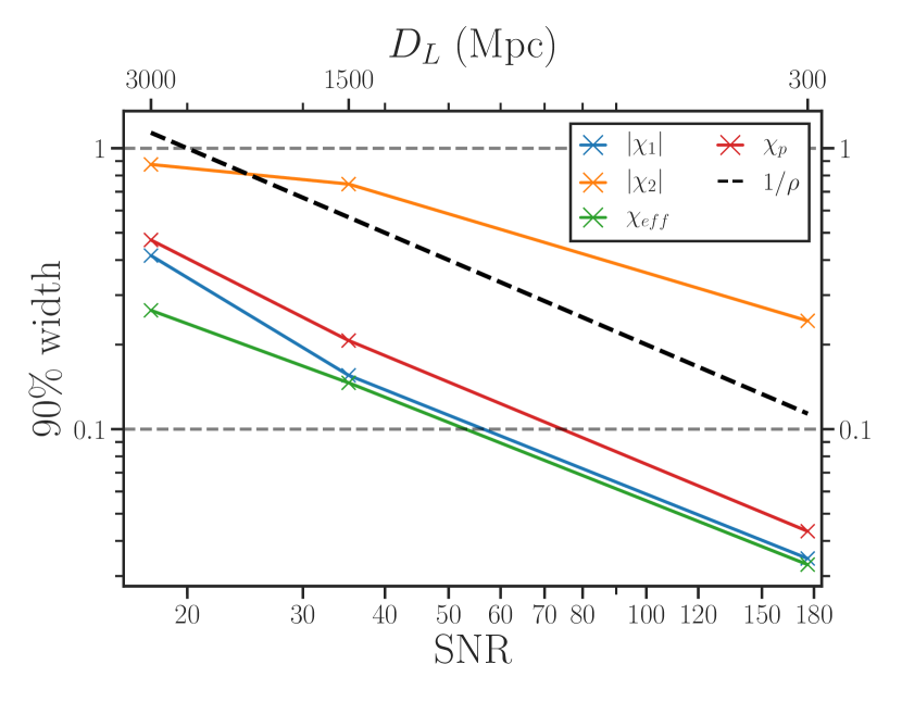
Figure 4: 90% credible intervals for the BH spin magnitudes and effective spin parameters as a function of injected SNR.

Figure 4 shows the primary and secondary spin magnitude $|\chi_{1}|,|\chi_{2}|$, the effective aligned-spin $\chi_{\rm{eff}}$ and effective precessing-spin $\chi_{\rm{p}}$ parameters.

With the exception of $|\chi_{2}|$ we find good agreement with the $1/\rho$ scaling. This suggests that for $|\chi_{2}|$ the two weaker injections do not have high enough SNR for the posterior distribution function for this parameter to be approximated by a Gaussian Vallisneri (2008). That being said, we do observe the 90% width decrease with SNR albeit at a slower rate. At SNR of $17$ and $34$ we find we are not able to place strong constraints on $|\chi_{2}|$ with $C_{90\%}^{17}(|\chi_{2}|)=0.87$ and $C_{90\%}^{34}(|\chi_{2}|)=0.77$. However, at the high SNR of $176$ we begin to constrain the spin magnitude at the level of $C_{90\%}^{176}(|\chi_{2}|)=0.24$, approximately the same level of uncertainty as $\chi_{\rm{eff}}$ at a SNR of 17. This is consistent with the study of non-precessing binaries in Ref. Purrer et al. (2016), which concluded that the secondary spin will not be measurable for SNRs below $\sim$100, but our results suggest that this carries over to precessing systems.

The primary spin magnitude is measured with much higher precision than the secondary spin magnitude. However, constraining this parameter to a 90% width of less than 0.2 requires an SNR of $\sim 30$. This parameter does follow the $1/\rho$ scaling very well and for high SNR cases we estimate the statistical uncertainty to be $C_{90\%}^{176}(|\chi_{1}|)=0.04$.

Of the effective spin parameters the effective aligned parameter $\chi_{\rm{eff}}$ is the best measured quantity. This is closely related to the leading order spin effect in Post Newtonian (PN) theory Poisson and Will (1995); Ajith (2011) appearing at 1.5 PN order. For all three SNRs the median value is always within $10^{-3}$ of the true value with the uncertainties ranging from $C_{90\%}^{17}(\chi_{\rm{eff}})=0.265$ to $C_{90\%}^{176}(\chi_{\rm{eff}})=0.033$.

Turning towards the effective precession spin parameter, $\chi_{p}$, at the lowest SNR we find the marginalised posterior for $\chi_{p}$ has a median value of $0.681$, close to the true value but with a wide uncertainty of $C_{90\%}^{17}(\chi_{p})=0.47$, spanning almost half of the full range. The evolution of the median value does not change significantly with increasing SNR however, our measurement uncertainty does decrease with increasing SNR as expected and we find $C_{90\%}^{35}(\chi_{p})=0.203$ for the medium SNR and $C_{90\%}^{176}(\chi_{p})=0.044$ for the high SNR case.

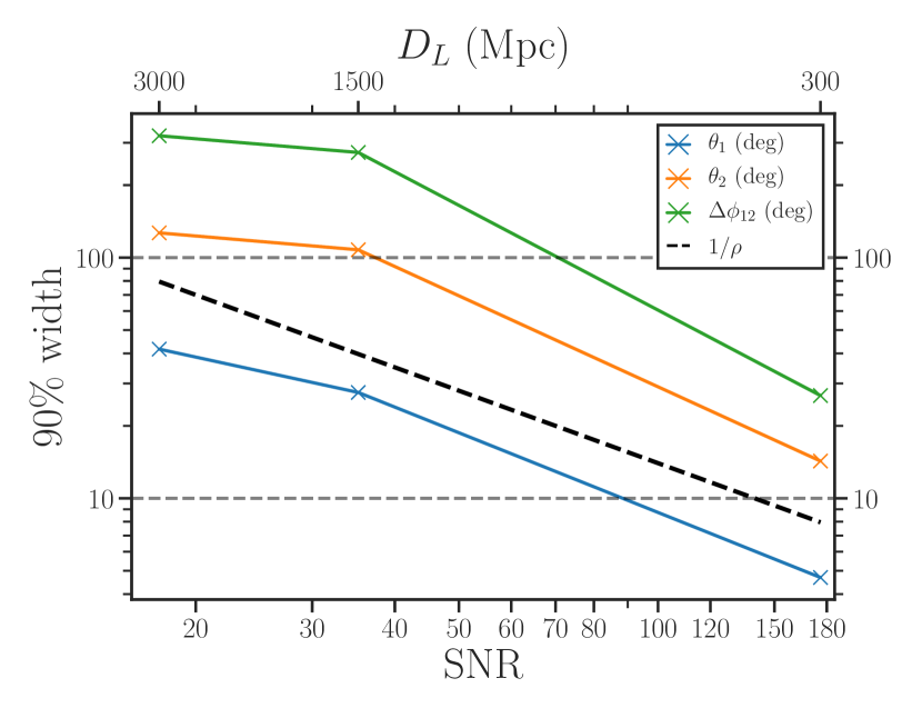
Figure 5: 90% credible intervals for the BH spin orientation parameters as a function of injected SNR.

Figure 5 shows the spin orientation parameters. $\theta_{1}$ and $\theta_{2}$ are the polar angles of the primary and secondary spin vectors with respect to the orbital angular momentum at the reference frequency. The angle $\Delta\phi_{12}$ is the angle between the primary and secondary spin vectors projected into the instantaneous orbital plane at the reference frequency. This angle is particularly useful when characterising precessing binaries as $\Delta\phi_{12}=0$ or $\Delta\phi_{12}=\pi$ are resonant spin configurations (if other conditions on the mass-ratio and spin magnitudes are met) Schnittman (2004).

We find $\theta_{1}$ has good SNR scaling with $C_{90\%}^{17}(\theta_{1})=0.73$ rad ($\sim 42$ deg) and $C_{90\%}^{176}(\theta_{1})=0.08$ rad ($\sim 5$ deg). Furthermore, $\theta_{2}$ and $\Delta\phi_{12}$ are measured much less accurately and require SNRs of $\sim 60$ and $\sim 100$ to achieve statistical uncertainties of $\sim 1$ rad ($\sim 60$ deg), respectively. However, in the event of a high SNR signal we find we are able to constrain $\theta_{2}$ to $C_{90\%}^{176}(\theta_{2})=0.26$ rad ($\sim 15$ deg) and $\Delta\phi_{12}$ to $C_{90\%}^{176}(\Delta\phi_{12})=0.48$ rad ($\sim 28$ deg).

In summary, we find that the primary spin magnitude $|\chi_{1}|$ and polar angle $\theta_{1}$ can be constrained at an SNR of $\sim 30$, while the seconday spin magnitude $|\chi_{2}|$ and polar angle $\theta_{2}$, as well as the the information about the relative orientation of the spin vectors $\Delta\phi_{12}$ are not constrained until we reach an SNR of $\sim 200$.

III.2.3 Waveform Systematics

Parameter estimation on a GW event with a waveform model that does not include relevant physics effects could result in biased results. To quantify the size of the bias due to neglecting higher modes and/or precession for this signal we repeat our parameter estimation analsis with four additional models.

The waveform models we use are listed in Tab. 4, where we mark whether or not each model contains precession and/or higher modes. PhenomD is the baseline model upon which the other Phenom models used in this work are built. We include two different precessing models PhenomPv2 and PhenomPv3 to gauge systematics on precession. PhenomHM includes higher modes but is a non-precessing model and finally the precessing and higher mode model PhenomPv3HM presented in this article.

Our results are presented in Fig. 6. From left to right the columns show the one dimensional marginalised posterior distribution for the; $m_{1}^{det}$, $m_{2}^{det}$, $\chi_{\rm{eff}}$ and $\chi_{\rm{p}}$. The rows from top to bottom show the results for the low $(\rho=17)$, medium $(\rho=34)$ and high $(\rho=176)$ SNR injections. The true value is shown as a vertical dashed black line. For all SNRs we find biases in the recovered masses for all models other than PhenomPv3HM i.e., the model that was used to produce the synthetic signal. This suggests that for real GW signals that are similar to this injection require analysis with models that contain both the effects of precession and higher modes. For the high SNR case multi-mode posteriors are found for the PhenomD case. For $\chi_{\rm{eff}}$ we find that for the low SNR injection the true value is within the $90\%$ credible interval (CI) and therefore not considered biased however, as the SNR of the injection is increased we find that $\chi_{\rm{eff}}$ can become heavily biased for the two precessing models but remains unbiased for the non-precessing models. For $\chi_{\rm{p}}$ we find that the precessing and non-higher mode models (PhenomPv2 and PhenomPv3) consistently favour larger values of $\chi_{\rm{p}}$ as the SNR increases. Interestingly we also start to find large differences between PhenomPv2 and PhenomPv3 at the high SNR cases.

Model	Precession	Higher Modes
PhenomD Husa et al. (2016); Khan et al. (2016)	✗	✗
PhenomPv2 Hannam et al. (2014); Schmidt et al. (2015)	✓	✗
PhenomPv3 Khan et al. (2019)	✓	✗
PhenomHM London et al. (2018)	✗	✓
PhenomPv3HM	✓	✓

Table 4: Waveform models that we use to analyse GW170729 and highlighting which physical effects are included each model.

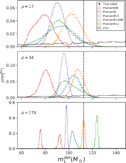
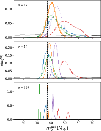
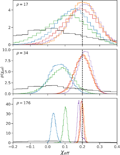
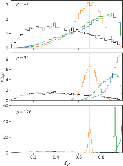
Figure 6: One dimensional marginal posterior probability distributions for detector-frame primary and secondary masses (1st and 2nd columns respectively), effective aligned-spin $\chi_{\rm{eff}}$ and effective precession spin $\chi_{\rm{p}}$ parameters (3rd and 4th columns respectively). Each row, from top to bottom, shows results for the low $(\rho=17)$, medium $(\rho=34)$ and high $(\rho=176)$ SNR injections. The true value is marked as a vertical black dashed line. The prior is shown as a black historgram. We show results for PhenomD (red), PhenomHM (purple), PhenomPv2 (green), PhenomPv3 (blue) and PhenomPv3HM (orange). Note the results for $\chi_{\rm{p}}$ do not show PhenomD or PhenomHM as they are aligned-spin models only.

III.3 GW170729 Analysis

Of the ten binary-black-hole observations reported by the LIGO-Virgo collaborations Abbott et al. (2018a), GW170729 shows the strongest evidence for unequal masses, making it the most likely signal for which higher modes could impact parameter measurements. This motivated the study in Ref. Chatziioannou et al. (2019), where the authors analysed GW170729 with two new aligned-spin and higher mode models (SEOBNRv4HM Cotesta et al. (2018) and PhenomHM London et al. (2018)). They found that the models preferred to interpret the data as the GW signal coming from a higher mass-ratio system with estimates for the mass-ratio changing from $0.62^{+0.36}_{-0.23}$ for PhenomPv2 to $0.52^{+0.26}_{-0.21}$ for PhenomHM ($90\%$ credible interval). This event also has evidence for a positive $\chi_{\rm{eff}}$, although when analysed with higher modes the $90\%$ credible interval for $\chi_{\rm{eff}}$ extended to include zero. This event has also been analysed in Payne et al. (2019) with the aligned-spin and higher mode model NRHybSur3dq8 Varma et al. (2019a) where the the authors draw similar conclusions. Motivated by this we prioritise GW170729 to analyse first with PhenomPv3HM and compare to existing results. We use the posterior samples for PhenomHM from Chatziioannou et al. (2019), and for PhenomPv2 from gwt . Results for PhenomD, PhenomPv3 and PhenomPv3HM were computed for this work using the LALInferenceMCMC code Veitch et al. (2015b).

In Fig. 7 we show the joint posterior for the source frame component masses ($m^{\rm{src}}_{1}$, $m^{\rm{src}}_{2}$) in the upper left; the aligned effective spin and mass-ratio ($\chi_{\rm{eff}}$, $q$) in the upper right and finally the luminosity distance and inclination angle ($D_{L}$, $\iota$) in the bottom plot. The quantitative parameter estimates for the source properties are provided in Tab. 5. Our posterior on the effective precession parameter $\chi_{p}$ is consistent with previous results and shows no significant differences due to different choice of precession model (between PhenomPv2 and PhenomPv3) or including both precession and higher modes as in PhenomPv3HM. We find that the marginal posterior effective aligned-spin parameter $\chi_{\rm{eff}}$ and luminosity distance $D_{L}$ are remarkably similar to the results from PhenomHM. The posterior for the inclination angle $\iota$ for IMPhenomPv3HM has more support for more inclined viewing angles; however, the change is minor.

Interestingly, not only do we find remarkably consistent results between PhenomD and PhenomPv2 as discussed in Chatziioannou et al. (2019) but also with PhenomPv3. This indicates that precession alone does not influence our inference for this event. However, including precession in addition to higher modes in the analysis does noticeably shift the posterior, albeit not very significantly in terms of the 90% CIs, which mostly overlap.

We find that the one-dimensional marginal posterior for the mass-ratio is pushed further towards lower mass-ratio values (more asymmetric) when using PhenomPv3HM where we find $q=0.47^{+0.28}_{-0.16}$ ($90\%$ level), implying that including precession and higher modes reinforces the findings of  Chatziioannou et al. (2019). As more asymmetric masses are favoured the estimate for the primary mass (source frame) is shifted towards higher values and the secondary mass is shifted towards lower values where we find $m_{1}^{src}=58.25^{+11.73}_{-12.53}M_{\odot}$ and $m_{2}^{src}=28.18^{+9.83}_{-7.65}M_{\odot}$.

By favouring larger mass estimates for the primary BH we challenge formation models to describe this event through standard stellar evolution mechanisms. In particular our results inform the pulsational pair-instability supernova (PPISN) mechanism Yoshida et al. (2016); Woosley (2017). The population synthesis analysis in Stevenson et al. (2019) investigated the resulting distribution of BH masses subject to different PPISN models. They find that in three out of the four models that they explore, the maximum BH mass is $\sim 40M_{\odot}$  Belczynski, K. et al. (2016); Marchant et al. (2018); Woosley (2019), and in one of the models the maximum BH mass is $\sim 58M_{\odot}$  Woosley (2017). In Fig. 8 we show the one-dimensional marginal posterior for the source-frame primary mass resulting from the analysis using PhenomPv2 (blue), PhenomHM (orange) and PhenomPv3HM (purple). The 90% credible interval of each result is shown as the shaded area under their respective curves. The vertical black dashed lines denote the maximum BH mass from the four different PPISN models that were investigated in Stevenson et al. (2019). We do not show the posterior for PhenomD or PhenomPv3 as these are consistent with the PhenomPv2 posterior.

When using PhenomPv2 to analyse the data we find that the maximum BH mass for all PPISN models are consistent with the posterior. When we include non-precessing, higher modes (PhenomHM) the PPISN models that predict maximum BH masses of $\sim 40M_{\odot}$  Belczynski, K. et al. (2016); Marchant et al. (2018); Woosley (2019) are excluded at the following level. In the posterior $1.3\%$ of samples have a mass of $\leqslant 40M_{\odot}$. As noted previously when we include both precession and higher modes the primary mass shifts slightly higher resulting in $0.6\%$ of samples having a mass of $\leqslant 40M_{\odot}$. If we assume that the primary BH in the GW170729 binary underwent a PPISN then the following PPISN models Belczynski, K. et al. (2016); Marchant et al. (2018); Woosley (2019) are disfavoured at greater than 90% credibility and the maximum BH mass as predicted by Woosley (2017) is consistent with our results. There are some caveats to these results however. In Stevenson et al. (2019) the authors uses a linear fit to the PPISN model of Woosley (2017) that systematically predicts larger remnant BH masses for pre-supernova helium (core) masses $M_{\rm{He}}>60M_{\odot}$ than the model of Woosley (2017) predicts. This in turn leads to larger maximum BH masses for this particular model. However, the size of this systematic uncertainty is unknown. Another caveat in the analysis of Stevenson et al. (2019) is that the models Marchant et al. (2018); Woosley (2019) have an uncertianty of $\sim 5M_{\odot}$ to account for the difference between the gravitational and baryonic mass Fryer et al. (2012).

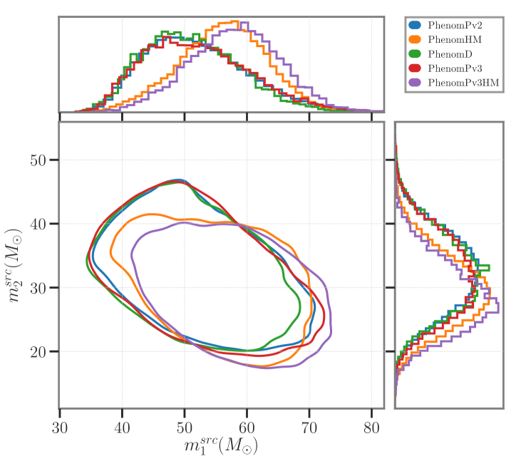
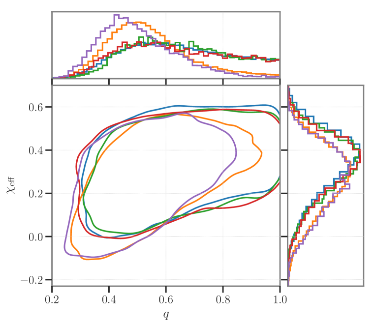
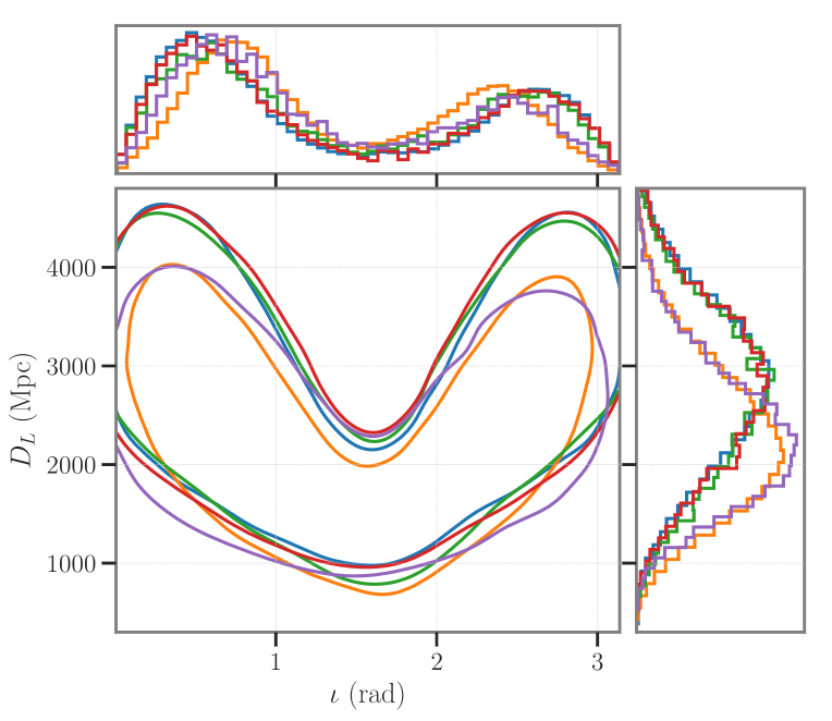
Figure 7: GW170729 parameter estimation results. Top left: component source-frame masses ($m^{\rm{src}}_{1}$, $m^{\rm{src}}_{2}$). Top right: effective spin and mass-ratio ($\chi_{\rm{eff}}$, $q$). Bottom: inclination angle and luminosity distance ($\iota$, $D_{L}$). The contour lines correspond to a credible level of $90\%$.

Parameter	PhenomD	PhenomHM	PhenomPv2	PhenomPv3	PhenomPv3HM
Primary Source Mass: $m^{\rm{src}}_{1}/M_{\odot}$	$50.55^{+14.02}_{-10.64}$	$56.36^{+11.08}_{-12.41}$	$51.22^{+16.19}_{-10.99}$	$51.39^{+16.35}_{-11.58}$	$58.25^{+11.73}_{-12.53}$
Secondary Source Mass: $m^{\rm{src}}_{2}/M_{\odot}$	$32.18^{+10.18}_{-8.84}$	$29.45^{+9.72}_{-8.36}$	$32.43^{+9.75}_{-9.46}$	$31.67^{+10.43}_{-9.27}$	$28.18^{+9.83}_{-7.65}$
Total Source Mass: $M_{\rm{total}}^{\rm{src}}/M_{\odot}$	$82.80^{+15.29}_{-10.82}$	$85.16^{+14.00}_{-10.53}$	$83.93^{+14.74}_{-10.91}$	$83.52^{+14.94}_{-11.09}$	$86.18^{+13.42}_{-10.77}$
Mass-Ratio: $q$	$0.64^{+0.31}_{-0.24}$	$0.52^{+0.31}_{-0.18}$	$0.63^{+0.32}_{-0.26}$	$0.62^{+0.33}_{-0.26}$	$0.48^{+0.28}_{-0.16}$
Effective Aligned Spin: $\chi_{\rm{eff}}$	$0.34^{+0.19}_{-0.26}$	$0.28^{+0.22}_{-0.28}$	$0.36^{+0.19}_{-0.28}$	$0.34^{+0.19}_{-0.27}$	$0.27^{+0.21}_{-0.28}$
Effective Precession Spin: $\chi_{\rm{p}}$	N/A	N/A	$0.44^{+0.35}_{-0.29}$	$0.44^{+0.36}_{-0.30}$	$0.42^{+0.39}_{-0.29}$
Luminosity Distance: $D_{L}$ / Mpc	$2749^{+1353}_{-1359}$	$2241^{+1391}_{-1065}$	$2831^{+1371}_{-1340}$	$2797^{+1386}_{-1318}$	$2270^{+1307}_{-974}$
redshift: $z$	$0.48^{+0.19}_{-0.21}$	$0.40^{+0.20}_{-0.17}$	$0.49^{+0.19}_{-0.21}$	$0.48^{+0.19}_{-0.20}$	$0.41^{+0.19}_{-0.16}$

Table 5: Parameter estimation results for GW170729. Masses are quoted in the source frame. We quote the median and the 90% symmetric credible interval of the one-dimensional marginalised posterior distributions.

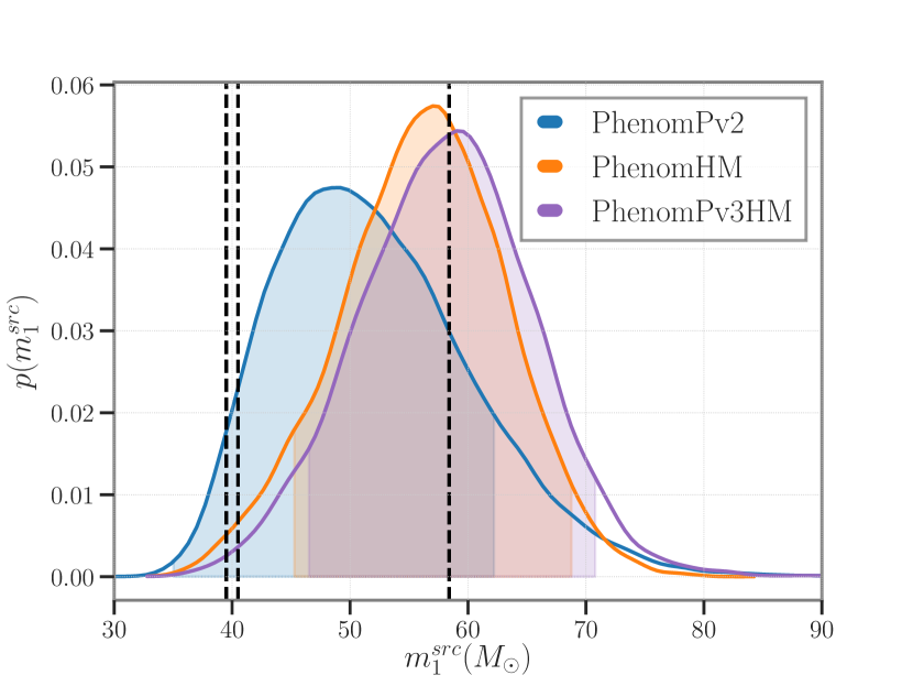
Figure 8: one-dimensional marginal posterior distribution for the primary source-frame mass. The posteriors for three waveform models are shown: PhenomPv2 (blue), PhenomHM (orange) and PhenomPv3HM (purple). The 90% credible interval of each result is shown as the shaded area under their respective curves. We also plot as vertical black dashed lines the maximum BH mass from four different PPISN models, which were investigated in Ref. Stevenson et al. (2019). Ref. Woosley (2017) predict a maximum mass of $58.4M_{\odot}$, Ref. Belczynski, K. et al. (2016) predicts $40.5M_{\odot}$ and Refs. Marchant et al. (2018); Woosley (2019) both predict $39.5M_{\odot}$.

IV Discussion and Future

In this work we have presented the first, frequency-domain, phenomenological IMR model for spin-precessing BBHs that also includes the effects of subdominant multipoles — beyond the quadrupole — in the co-precessing frame. By comparing to a large set of precessing NR simulations we find that our simple model is able to accurately reproduce the expected GW signal with an accuracy of $99\%$ ($97\%$) for small (high) inclinations, a significant improvement over models that do not include subdominant multipoles, which have accuracies of $97\%$ ($91\%$) for small (high) inclinations.

Precise measurements of BH spins from GW observations requires high SNR events in part due to the relatively high PN order that spin effects appear at. We performed an idealized parameter estimation analysis to quantify the precision to which the BH spin magnitude and orientation can be measured, ignoring any effects of systematic error on the waveform. We find, for this particular system (See Table 2), that the primary spin parameters are more tightly constrained than the secondary spin, as expected for an unequal-mass system such as this. In the following discussion we remind the reader that the low, medium and high SNR cases have corresponding values of $17$, $34$ and $176$ respectively. The primary spin magnitude can be constrained to a 90% CI of $0.42$ for the low SNR case (about half the width of the physical range) and to a 90% CI of $0.04$ for the high SNR case. The secondary spin magnitude cannot be meaningfully constrained until the high SNR case with a 90% CI of $0.24$. The primary spin polar angle shows reasonably good agreement with the expected SNR scaling and can be constrained to $\sim 42$ deg (low SNR) and $\sim 5$ deg (high SNR) at 90% CI. The secondary spin polar angle shows poor agreement with the expected SNR scaling and we find can only be meaningfully constrained ($\sim 15$ deg) for the high SNR case. The azimuthal angle between the spins ($\Delta\phi_{12}$) shows poor scaling with SNR. We find that only the highest SNR case was able to constrain $\Delta\phi_{12}\lesssim 28$ deg. Our parameter estimation study is only a point estimate for the size of the uncertainty on binary properties and a systematic study that explores the parameter space of precessing binaries is required to draw more general conclusions Vitale et al. (2017); Vitale and Evans (2017). However, recent work in understanding precession better may help make such a study tractable by focusing on regions where we expect precession to be measurable Fairhurst et al. (2019a, b).

We have analysed the GW event GW170729 with the new precessing and higher mode model. We have shown that while the general interpretation of this event is unchanged we find that even small shifts in the posteriors due to using different waveform models, with different physical effects incorporated, can be enough to inform astrophysical models such as the PPISN mechanism as we considered in this paper. If we assume that the primary BH in the GW170729 binary underwent a PPISN then we disfavour the PPISN models from Belczynski, K. et al. (2016); Marchant et al. (2018); Woosley (2019) at greater than 90% credibility and our results are consistent with Woosley (2017). See Farmer et al. (2019) for a recent investigation into the location of the PPISN model mass-gap.

Our model is analytic and natively in the frequency-domain, and as such it can be readily used in likelihood acceleration methods such as reduced order quadrature (ROQ) Smith et al. (2016) or “multibanding” techniques Vinciguerra et al. (2017). This model can be used to determine the impact on GW searches, event parameter estimation and population inference due to the effects of precession and higher modes.

We expect to be able to greatly improve PhenomPv3HM, and similar models, by using models for the underlying higher multipole aligned-spin model that have been calibrated to NR waveforms García Quirós et al. (prep). Likewise, a model for the precession dynamics tuned to precessing NR simulations will improve its performance Hamilton et al. (prep). Although our model is a function of the 7 dimensional intrinsic parameter space of non-eccentric BBH mergers it is not 7 dimensional across the entire coalescence. It is true during the inspiral, but during the pre-merger and merger we use an effective aligned-spin parametrization. Work is underway to develop an NR calibrated aligned-spin model with the effects of two independent aligned-spins Geraint et al. (prep). In addition, promising attempts to dynamically enhance incomplete models via singular-value-decomposition have recently been presented Setyawati et al. (2019), and the model introduced here can easily be employed by such an automated tuning process.

With regards to higher modes we only include a subset of the complete list of modes, specifically $(\ell,|m|)=((2,2),(2,1),(3,3),(3,2),(4,4),(4,3))$. We also ignore mode mixing Berti and Klein (2014) and the asymmetry between the $+m$ and $-m$ modes, which are responsible for out of plane recoils Bruegmann et al. (2008).

We plan to extend this model to include tidal effects as introduced in Dietrich et al. (2018, 2019) as well as implement a model for the GW suitable for neutron star-black hole binaries where the effects of spin-precession, subdominant multipoles and tidal effects could all become important. The model presented here could be used as a baseline for such a model. Finally this model is implemented in the LSC Algorithm Library (LAL) LIGO Scientific Collaboration (2018).