Multi-Label Learning with Deep Forest

Abstract

In multi-label learning, each instance is associated with multiple labels and the crucial task is how to leverage label correlations in building models. Deep neural network methods usually jointly embed the feature and label information into a latent space to exploit label correlations. However, the success of these methods highly depends on the precise choice of model depth. Deep forest is a recent deep learning framework based on tree model ensembles, which does not rely on backpropagation. We consider the advantages of deep forest models are very appropriate for solving multi-label problems. Therefore we design the Multi-Label Deep Forest (MLDF) method with two mechanisms: measure-aware feature reuse and measure-aware layer growth. The measure-aware feature reuse mechanism reuses the good representation in the previous layer guided by confidence. The measure-aware layer growth mechanism ensures MLDF gradually increase the model complexity by performance measure. MLDF handles two challenging problems at the same time: one is restricting the model complexity to ease the overfitting issue; another is optimizing the performance measure on user’s demand since there are many different measures in the multi-label evaluation. Experiments show that our proposal not only beats the compared methods over six measures on benchmark datasets but also enjoys label correlation discovery and other desired properties in multi-label learning.

   

1 Introduction

In multi-label learning, each example is associated with multiple labels simultaneously and the task of multi-label learning is to predict a set of relevant labels for the unseen instance. Multi-label learning has been widely applied in diverse problems like text categorization [Zhou and El-Gohary, 2015], scene classification [Zhao et al., 2015], functional genomics [Zhang and Zhou, 2006], video categorization [Ray et al., 2018], chemicals classification [Cheng et al., 2017], etc. It is drawn increased research attention that multi-label learning tasks are omnipresent in real-world problems [Tsoumakas et al., 2010].

By transforming the multi-label learning problem to independent binary classification problems for each label, Binary Relevance [Tsoumakas and Katakis, 2007] is a straightforward method which has been widely used in practice. Though it aims to make full use of high-performance traditional single-label classifiers, it will lead to high computational cost when label space is large. Besides, such a method neglects the fact that information on one label may be helpful for learning other related labels, which would limit the prediction performance. Investigating correlations among labels has been demonstrated to be the key to improve the performance of multi-label learning. As a result, more and more multi-label learning methods aim to explore and exploit the label correlations are proposed [Tsoumakas et al., 2010]. There emerges considerable attention in exploring and exploiting label correlations in multi-label learning methods [Tsoumakas et al., 2010; Wang et al., 2016; Zhang et al., 2018a].

Different from traditional multi-label methods, deep neural network models usually try to learn a new feature space and employ a multi-label classifier on the top. Among the first to utilize network architectures, BP-MLL [Zhang and Zhou, 2006] not only treats each output node as a binary classification task but also exploits label correlations relied on the architecture itself. Later, a comparably simple Neural Network approach builds upon BP-MLL was proposed by replacing the pairwise ranking loss with entropy loss and using deep neural networks techniques [Nam et al., 2014] and it achieves a good result in the large-scale text classification. However, deep neural models usually require a huge amount of training data, and thus they are generally not suitable for small-scale datasets.

By realizing that the essence of deep learning lies in layer-by-layer processing, in-model feature transformation, and sufficient model complexity, Zhou and Feng proposed deep forest [Zhou and Feng, 2018]. Deep forest is an ensemble deep model built on decision trees and does not use backpropagation in the training process. A deep forest ensembled with a cascade structure is able to do representation learning similarly like deep neural models. Deep forest is much easier to train since it has fewer hyper-parameters. It has achieved excellent performance on a broad range of tasks, such as large-scale financial fraud detection [Zhang et al., 2018b], image, and text reconstruction [Feng and Zhou, 2018]. Though deep forest has been found useful in traditional classification tasks [Zhou and Feng, 2018], the potential of applying it into multi-label learning has not been noticed before our work.

The success of deep forest mainly comes from the layer-by-layer feature transformation in an ensemble way [Zhou, 2012]. While on the other hand, the key point in multi-label learning is how to use label correlations. Inspired by these two facts, we propose the Multi-Label Deep Forest (MLDF) method. Briefly speaking, MLDF uses different multi-label tree methods as the building blocks in deep forest, and label correlations can be exploited via layer-by-layer representation learning. Because evaluation in multi-label learning is more complicated than traditional classification tasks, a number of performance measures have been proposed [Schapire and Singer, 2000]. It is noticed that ifferent user has different demands and an algorithm usually performs differently on different measures [Wu and Zhou, 2017]. In order to achieve better performance on the specific measure, we propose two mechanisms: measure-aware feature reuse and measure-aware layer growth. The measure-aware feature reuse mechanism, inspired by confidence screening [Pang et al., 2018], reuses good presentation in the previous layer. The measure-aware layer growth mechanism aims to control the model complexity by various performance measures. The main contributions of this paper are summarized as follows:

• We first introduce deep forest to multi-label learning. Because of the proposed cascade structure and two measure-aware mechanisms, our MLDF method can handle two challenging problems in multi-label learning at the same time: optimizing different performance measures on user demand, and reducing overfitting, when utilizing label correlations by a large number of layers, which often observed in deep neural multi-label models.

• Our extensive experiments show that MLDF achieves the best performance on 9 benchmark datasets over 6 multi-label measures. Besides, the two mechanisms are confirmed necessary in MLDF. Furthermore, investigative experiments demonstrate our proposal enjoys high flexibility in applying various base tree models and resistance to overfitting.

The remainder of the paper is organized as follows. Section 2 introduces some preliminaries. Section 3 formally describes our MLDF method and two measure-aware mechanisms. Section 4 reports the experimental results on benchmarks and investigative experiments. Finally, we conclude the paper in Section 5.

2 PRELIMINARIES

In this section, we introduce various performance measures, followed by the tree-based multi-label methods, which are the base of Multi-Label Deep Forest.

2.1 Multi-label performance measures

The multi-label classification task is to derive a function $H$ from the training set $\{(\boldsymbol{x}_{i},\boldsymbol{y}_{i})|1\leq i\leq m,\boldsymbol{x}_{i}\in\mathbb{R}^{d},\boldsymbol{y}_{i}\in\{0,1\}^{l}\}$. Suppose the multi-label learning model first produces a real-valued function $F:\mathcal{X}\rightarrow[0,1]^{l}$, which can be viewed as the confidence of relevance of the labels. The multi-label classifier $H:\mathcal{X}\rightarrow\{0,1\}^{l}$ can be induced from $F$ by thresholding.

There are lots of performance measures for multi-label learning. Six widely-used evaluation measures are employed in this paper [Wu and Zhou, 2017]. Table 1 shows the formulation of these measures, being $Y$ the true labels, $Y_{i\cdot}$ the $i$-th row of the label matrix, ‘$+$’(‘$-$’) the relevant (irrelevant) note. Hamming loss and macro-AUC are label-based measures, while one-error, coverage, ranking loss and average precision are instance-based measures [Zhang and Zhou, 2014]. The $f_{ij}$ means the confidence score of $i$-th instance on $j$-th label, $h_{ij}$ means the predict result of $i$-th instance on $j$-th label, and $\mathrm{rank}_{F}\left(\boldsymbol{x}_{i},j\right)$ means the instance $\boldsymbol{x}_{i}$’s rank on $j$-th label. For example, $\boldsymbol{f}(\boldsymbol{x_{i}})=[0.2,0.8,0.4]$, then we have $\boldsymbol{h}(\boldsymbol{x_{i}})=[0,1,0]$ with threshold 0.5. Furthermore, we have $Y_{i\cdot}^{-}=\{1,3\}$ and $Y_{i\cdot}^{+}=\{2\}$. Since $f_{i2}=0.8$, then we have $\mathrm{rank}_{F}(\boldsymbol{x}_{i},2)=1$.

Table 1: Definitions of six multi-label performance measures, ‘$\downarrow$’ means the lower the better, ‘$\uparrow$’ means the higher the better.

Measure	Formulation
hamming loss $\downarrow$	$\frac{1}{ml}\sum\limits_{i=1}^{m}\sum\limits_{j=1}^{l}\mathbb{I}[h_{ij}\neq y_{ij}]$
one-error $\downarrow$	$\frac{1}{m}\sum\limits_{i=1}^{m}\mathbb{I}\left[\arg\max F\left(\boldsymbol{x}_{i}\right)\notin Y_{i\cdot}^{+}\right]$
coverage $\downarrow$	$\frac{1}{ml}\sum\limits_{i=1}^{m}\mathbb{I}\left[\max\limits_{j\in Y_{i\cdot}^{+}}\mathrm{rank}_{F}\left(\boldsymbol{x}_{i},j\right)-1\right]$
ranking loss $\downarrow$	$\frac{1}{m}\sum\limits_{i=1}^{m}\frac{\left|\mathcal{S}_{\mathrm{rank}}^{i}\right|}{\left|Y_{i\cdot}^{+}\right|\left|Y_{i\cdot}^{-}\right|}$
average precision $\uparrow$	$\frac{1}{m}\sum\limits_{i=1}^{m}\frac{1}{\left|Y_{i\cdot}^{+}\right|}\sum\limits_{j\in Y_{i\cdot}^{+}}\frac{\left|\mathcal{S}_{\mathrm{precision}}^{ij}\right|}{\mathrm{rank}_{F}\left(\boldsymbol{x}_{i},j\right)}$
macro-AUC $\uparrow$	$\frac{1}{l}\sum\limits_{j=1}^{l}\frac{\left|\mathcal{S}_{\mathrm{macro}}^{j}\right|}{\left|Y_{\cdot i}^{+}\right|\left|Y_{\cdot i}^{-}\right|}$
$\mathcal{S}_{\mathrm{rank}}^{i}=\{(u,v)\in Y_{i}^{+}\times Y_{i}^{-}|f_{u}\left(\boldsymbol{x}_{i}\right)\leq f_{v}\left(\boldsymbol{x}_{i}\right)$}
$\mathcal{S}_{\mathrm{precision}}^{ij}=\left\{k\in Y_{i}^{+}|\mathrm{rank}_{F}\left(\boldsymbol{x}_{i},k\right)\leq\mathrm{rank}_{F}\left(\boldsymbol{x}_{i},j\right)\right\}$
$\mathcal{S}_{\mathrm{macro}}^{j}=\left\{(a,b)\in Y_{\cdot j}^{+}\times Y_{\cdot j}^{-}|f_{j}\left(\boldsymbol{x}_{a}\right)\geq f_{j}\left(\boldsymbol{x}_{b}\right)\right\}$

2.2 Tree-based multi-label methods

Tree-based multi-label methods, such as ML-C4.5 [Clare and King, 2001] and PCT [Blockeel et al., 1998], are adapted from multi-class tree methods. ML-C4.5, adapted from C4.5, allows multiple labels in the leaves of the tree, whose formula of entropy calculation is modified by summing the entropy for each label. Predictive Clustering Tree (PCT) recursively partitions all samples into smaller clusters while moving down the tree. In the testing process, the leaf node of a multi-label tree returns a vector of probabilities that a sample belongs to each class, by counting the percentage of different classes of training examples at the leaf node where concerned instance falls. Finally, the information kept in each leaf node is the probability that the instance owns each label.

The ability of a single tree is limited, but ensemble of the trees will greatly improve performance. Random Forest of Predictive Clustering Trees (RF-PCT) [Kocev et al., 2013] and Random Forest of ML-C4.5 (RFML-C4.5) [Madjarov et al., 2012] are ensembles that use PCT and ML-C4.5 as base classifiers respectively. The same as random forest, these forests use bagging and choose different feature sets to obtain the diversity among the base classifiers. Given a test instance, the forest will produce an estimate of label distribution by averaging results across all trees.

3 THE PROPOSED METHOD

In this section, we propose a deep forest method for multi-label learning. Firstly, we introduce the framework of Multi-Label Deep Forest (MLDF). Then, we discuss two proposed mechanisms: measure-aware feature reuse and measure-aware layer growth.

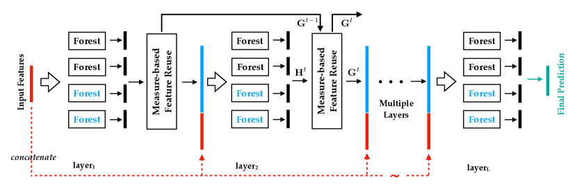
Figure 1: The framework of Multi-Label Deep Forest (MLDF). Each layer ensembles two different forests (the black above and the blue below).

3.1 The framework

Figure 1 illustrates the framework of MLDF. Different multi-label forests (the black forests above and the blue forests below) are ensembled in each layer of MLDF. From $\mathrm{layer}_{t}$, we can obtain the representation $\mathbf{H}^{t}$. The part of measure-aware feature reuse will receive the representation $\mathbf{H}^{t}$ and update it by reusing the representation $\mathbf{G}^{t-1}$ learned in the $\mathrm{layer}_{t-1}$ under the guidance of the performance of different measures. Then the new representation $\mathbf{G}^{t}$ (the blue one) will be concatenated together with the raw input features (the red one) and goes into the next layer.

In MLDF, each layer is an ensemble of forests. To enhance the performance of the ensemble, we consider different growing methods of trees to encourage diversity, which is crucial in the success of ensemble methods [Zhou, 2012]. In traditional multi-class problems, extremely-random trees [Geurts et al., 2006], which takes one split point of each feature randomly, are used in gcForest [Zhou and Feng, 2017]. For multi-label learning problems, we can also adapt this kind of method by changing the approach of splitting nodes when generating trees. In MLDF, we take RF-PCT [Kocev et al., 2013] as the forest block, and two different methods generating nodes in trees are used to forests: one considers all possible split point of each feature, which is RF-PCT, the other considers one split point randomly [Kocev and Ceci, 2015], we name this as ERF-PCT. Of course, other multi-label tree methods can also be embedded into each layer such as RFML-C4.5, which will be discussed in Section 4.

As aforementioned in Section 2.2, given an instance, the forests will produce an estimation of label distributions, which can be viewed as the confidence of the instance belonging to each label. The representation learned in each layer will adopt measure-aware feature reuse and be input to the next layer with raw input features. The real-valued representation with rich labeling information will be input to the next layer to facilitate MLDF to take better advantage of label correlations [Belanger et al., 2017].

The predicting process can be summarized as follows. As shown in Figure 1, assume the forests have been fitted well. Firstly, we pre-process instances to standard matrix $\mathbf{X}$. Secondly, the instances matrix $\mathbf{X}$ passes the first layer, and we can get the representation $\mathbf{H}^{1}$. By adopting measure-aware feature reuse, we can get $\mathbf{G}^{1}$. Then we concatenate $\mathbf{G}^{1}$ with the raw input features $\mathbf{X}$ and put them into the next layer. After multiple layers, we get the final perdition.

Table 2: Confidence computing method on six multi-label measures. $\boldsymbol{p}_{i\cdot}$ or $\boldsymbol{p}_{\cdot j}$ is sorted in descending order.

Measure	Confidence
hamming loss	$\frac{1}{m}\sum\limits_{i=1}^{m}p_{ij}\mathbb{I}[p_{ij}>0.5]+(1-p_{ij})\mathbb{I}[p_{ij}\leq 0.5]$
		one-error	$\max\limits_{i=1,\dots,m}{p_{ij}}$
coverage	$1-\frac{1}{l}\sum\limits_{j=0}^{l}\left[j\cdot p_{ij}\prod\limits_{k=j+1}^{l}\left(1-p_{ik}\right)\right]$
		ranking loss	$\sum\limits_{j=0}^{l}\prod\limits_{k=1}^{j}p_{ik}\prod\limits_{k=j+1}^{l}\left(1-p_{ik}\right)$
average precision	$\sum\limits_{j=0}^{l}\prod\limits_{k=1}^{j}p_{ik}\prod\limits_{k=j+1}^{l}\left(1-p_{ik}\right)$
		macro-AUC	$\sum\limits_{i=0}^{m}\prod\limits_{k=1}^{i}p_{kj}\prod\limits_{k=i+1}^{m}\left(1-p_{kj}\right)$

Algorithm 1 Measure-aware feature reuse

0:  measure $M$, forests’ output $\mathbf{H}^{t}$, previous $\mathbf{G}^{t-1}$.

0:  new representation $\mathbf{G}^{t}$.

0:   

1:  Initialize matrix $\mathbf{G}^{t}=\mathbf{H}^{t}$.

2:  if Measure $M$ is label-based then

3:     for  $j=1$ to $l$  do

4:        compute confidence $\alpha^{t}_{j}$ on $\mathbf{H}^{t}_{\cdot j}$

5:        Update $\mathbf{G}^{t}_{\cdot j}$ to $\mathbf{G}^{t-1}_{\cdot j}$ when $\alpha^{t}_{j}<\theta_{t}$.

6:     end for

7:  end if

8:  if Measure $M$ is instance-based then

9:     for  $i=1$ to $m$  do

10:        compute confidence $\alpha^{t}_{i}$ on $\mathbf{H}^{t}_{i\cdot}$

11:        Update $\mathbf{G}^{t}_{i\cdot}$ to $\mathbf{G}^{t-1}_{i\cdot}$ when $\alpha^{t}_{i}<\theta_{t}$.

12:     end for

13:  end if

Algorithm 2 Determine threshold

0:  measure $M$, forests’ output $\mathbf{H}^{t}$, ground-truth $\mathbf{Y}$, previous performance on $\mathrm{layer}_{t-1}$.

0:  threshold $\theta_{t}$.

0:   

1:  Initialize confidence set $\mathcal{S}=\emptyset$.

2:  if Measure $M$ is label-based then

3:     for  $j=1$ to $l$  do

4:        compute confidence $\alpha^{t}_{j}$ on $\mathbf{H}^{t}_{\cdot j}$.

5:        compute measure $m^{t}_{j}$ on $(\mathbf{H}^{t}_{\cdot j},\mathbf{Y}_{\cdot j})$.

6:        $\mathcal{S}=\mathcal{S}\cup\{\alpha^{t}_{j}\}$ when $m^{t}_{j}$ is worse than $m^{t-1}_{j}$.

7:     end for

8:  end if

9:  if Measure $M$ is instance-based then

10:     for  $i=1$ to $m$  do

11:        compute confidence $\alpha^{t}_{i}$ on $\mathbf{H}^{t}_{i\cdot}$.

12:        compute measure $m^{t}_{i}$ on $(\mathbf{H}^{t}_{i\cdot},\mathbf{Y}_{i\cdot})$.

13:        $\mathcal{S}=\mathcal{S}\cup\{\alpha^{t}_{i}\}$ when $m^{t}_{j}$ is worse than $m^{t-1}_{j}$.

14:     end for

15:  end if

16:  $\theta_{t}$ = Compute threshold on $\mathcal{S}$.

3.2 Measure-aware feature reuse

The split criterion of PCT is not directly related to the performance measure, and the representation $\mathbf{H}^{t}$ generated by each layer is same though the measure is different. Therefore we propose the measure-aware feature reuse mechanism to enhance the representation under the guidance of different measures. The key idea of measure-aware feature reuse is to partially reuse the good representation in the previous layer on the current layer if the confidence on the current layer is lower than a tehreshold determined in training, which can make the measure performance better. Therefore, the challenge lies in defining the confidence of specific multi-label measures on demand. Inspire by the confidence computing method on the multi-class classification problem [Pang et al., 2018], we design a confidence computing method on different multi-label measures.

Hamming loss cares the correctness of single bit, one-error cares the element closest to 1, and others cares the ranking permutation on each row or column. Therefore, the crucial step is designing reasonable methods to compute the confidence for various measures. Table 2 summarizes the computing method by considering the real meaning of each measure. Matrix $\mathbf{P}$ is the average of $\mathbf{H}^{t}$, and the element $p_{ij}$ represents $\mathrm{Pr}[\hat{y}_{ij}=1]$. For convenience, we arrange the element of each row (column) of $\mathbf{P}$ in descending order when the measure is instance-based (label-based). Specifically, for hamming loss, we compute the max confidence that the bit is positive or negative. For example, the prediction vector $\mathbf{p}_{\cdot j}=\left[0.9,0.6,0.4,0.3\right]$, thus the confidence is $\alpha_{j}=\frac{1}{4}(0.9+0.6+0.6+0.7)=0.7$. For ranking loss, we compute the probability that the ranking loss is zero, which means the positive labels are ahead of negative labels. For example, if the prediction vector $\mathbf{p}_{i\cdot}=\left[0.9,0.6,0.4,0.3\right]$, there will be 5 possible permutations of ground-truth leading to zero ranking loss: $\{0000,1000,1100,1110,1111\}$. Therefore, we can get the confidence by summing the probabilities in these five cases. The confidence of macro-AUC and average precision are defined in a similarity way.

Algorithm 1 summarizes the process of the measure-aware feature reuse. Due to the diversity between label-based measures and instance-based measures [Wu and Zhou, 2017], we need to deal with them separately. Specifically, the label-based measures compute the confidence on each column of $\mathbf{H}^{t}$ and the instance-based measures compute it on each row. After the confidence computing, we fix the previous representation $\mathbf{G}^{t-1}$ when the confidence $\alpha^{t}$ is below the threshold, and update $\mathbf{G}^{t}$ with the fixed ones.

The whole process of measure-aware feature reuse does not rely on true labels. We can judge the goodness of representation by a threshold determined in training process. As Algorithm 2 shows, we save the confidence $\alpha^{t}$ into set $\mathcal{S}$ if the evaluated performance measure goes worse at $\mathrm{layer}_{t}$. Then, the threshold $\theta_{t}$ is determined based on $\mathcal{S}$. Simply, we can take an average on $\mathcal{S}$. Because the meaning of confidence is consistent with the measure, the threshold $\theta_{t}$ can be effectively utilized in measure-aware feature reuse.

3.3 Measure-aware layer growth

Algorithm 3 Measure-aware layer growth

0:  maximal depth $T$, measure $M$, training data $\{\bf{X},\bf{Y}\}$.

0:  model set $S$, threshold set $\Theta$ and final layer index $L$.

0:   

1:  Initialize parameters:  performance in each layer $\boldsymbol{p}$[1:T], best performance on train set $p_{\mathrm{best}}$, the initial threshold $\theta_{1}=0$, the best performance layer index $L=1$, the model set $\mathcal{S}=\emptyset$.

2:  for  $t=1$ to $T$  do

3:     Train forests in $\text{layer}_{t}$ and get classifier $h_{t}$.

4:     Predict $\mathbf{H}_{t}=h_{t}([\mathbf{X},\mathbf{G}_{t-1}])$.

5:     $\theta_{t}=$ Determine Threshold (Algorithm 2) when $t>2$.

6:     $\mathbf{G}^{t}=$ measure-aware feature reuse (Algorithm 1).

7:     Compute performance $\boldsymbol{p}[t]$ on measure $M$ with $\mathbf{G}^{t}$.

8:     if  $\boldsymbol{p}[t]$ is better than $p_{\mathrm{best}}$  then

9:        Update best performance $p_{\mathrm{best}}=\boldsymbol{p}[t]$.

10:        Update the layer index of best performance $L=t$.

11:     else if  $p_{\mathrm{best}}$ is not updated in recent 3 layers  then

12:        break

13:     end if

14:     Add $\mathrm{layer}_{t}$ to model set: $\mathcal{S}=\mathcal{S}\cup\mathrm{layer}_{t}$.

15:  end for

16:  Keep $\{\mathrm{layer}_{1},\dots,\mathrm{layer}_{L}\}$ in model set $S$ and drop others $\{\mathrm{layer}_{L+1},\dots\}$.

Though the measure-aware feature reuse can effectively enhance the representation guided by various measures, the mechanism can not influence the layer growth and reduce the risk of overfitting that may occur in training process. In order to reduce overfitting and control the model complexity, we propose the measure-aware layer growth mechanism.

If we use the same data to fit forests and do predicting directly, the risk of overfitting will be increased [Platt et al., 1999]. MLDF uses the $k$-fold cross-validation to alleviate this issue. For each fold, we train the forests based on the training examples in other folds and make the prediction on the current fold. The layer’s representation is generated by concatenating the predictions from each forest.

MLDF is built layer by layer. Algorithm 3 summarizes the procedure of measure-aware layer growth used in training MLDF. The inputs are maximal depth of layers $T$, evaluation measure $M$, and the training data $\{\bf{X},\bf{Y}\}$. If the model has grown $T$ layers, the training process will stop. In general, we can choose one RF-PCT and one ERF-PCT in each layer and randomly select $\sqrt{d}$ number of features as candidates in each forest. All parameters of training forest in MLDF, such as the number of forests and the depth of trees, are pre-determined before training. As we hope each layer to learn different representations, we can set the maximum depth of tree in forests growing with the layer $i$, so does the number of trees, which can be set in advance. In the initialization step, the performance vector $\boldsymbol{p}$, which records the performance value on training data in each layer, should be initialized according to different measures. During each layer, we first fit the forests (line 3) and get the representation $\mathbf{H}^{t}$ (line 4). Then we should determine the threshold $\theta_{t}$ (line 5) and generate new representation by measure-aware feature reuse (line 6). Finally we add the $\mathrm{layer}_{t}$ to model set $\mathcal{S}$ (line 14).

The layer growth is measure-aware. After fitting one layer, we need to compute the evaluation measure. When the measure is not getting better in recent three layers (line 11), MLDF is forced to stop growing. At the same time, the layer index of best performance in training dataset should be recorded, which is useful in prediction. According to Occam’s razor rule, we prefer a simpler model when the performance is similar. While there is no clear improvement in performance, the final model set $\mathcal{S}=\{\mathrm{layer}_{1},\dots,\mathrm{layer}_{L}\}$ should be kept, and layers after will be dropped.

Different measures represent different user demands. We can set $M$ as the required measure according to different situations. Therefore, we can obtain the corresponding model for the specified measure. On one hand, the model complexity can be controlled by $M$. On the other hand, compared to other methods, like PCT, that cannot explicitly take the performance measure into consideration in the training process, MLDF is more flexible and has the ability to get better performance.

4 EXPERIMENTS

In this section, we conduct experiments with MLDF on different multi-label classification benchmark datasets. Our goal is to validate MLDF can achieve the best performance on different measures and the two measure-aware mechanisms are necessray. Moreover, we show the advantages of MLDF through more detailed experiments from various aspects.

4.1 Dataset and configuration

We choose 9 multi-label classification benchmark datasets from different application domains and with different scales. Table 3 presents the basic statistics of these datasets. All datasets are from a repository of multi-label datasets. The datasets vary in size: from 502 up to 43970 examples, from 68 up to 5000 features, and from 5 up to 201 labels. They are roughly organized in ascending order of the number of examples $m$, with eight of them being regular-scale, i.e., $m<5000$ and eight of them being large-scale, i.e., $m>5000$. For all experiments conducted below, 50% examples are randomly sampled without replacement to form the training set, and the rest 50% examples are used to create the test set.

Six evaluation measures, widely used in multi-label learning [Wu and Zhou, 2017], are employed in this paper: hamming loss, one-error, coverage, ranking loss, average precision, and macro-AUC. Note that the coverage is normalized by the number of labels and thus all the evaluation measures all vary between [0,1].

Hyper-parameters of MLDF is set as follows. We set the number of max layer ($T$) as 20 and take $M$ with the six measures discussed above respectively, which means we will get different models with different measures. We take one RF-PCT and one ERF-PCT in each layer and use the 5-fold cross-validation to avoid overfitting. In the first layer, we take 40 trees in each forest, and then take 20 more trees than the previous layer until the number of trees reaches 100, which can enable MLDF to learn different representations. Similarly, we set the max-depth as 3 in the first layer, and then take 3 more than the previous layer when layer increasing.

Table 3: Descriptions of the datasets in terms of the domain (Domain), number of examples ($m$), number of features ($d$) and number of labels ($l$).

Dataset	Domain	$m$	$d$	$l$
CAL500	music	502	68	174
enron	text	1702	1001	53
image	images	2000	294	5
scene	images	2407	1196	6
yeast	biology	2417	103	14
corel16k-s1	images	13766	500	153
corel16k-s2	images	13761	500	164
eurlex-sm	text	19348	5000	201
mediamill	multimedia	43970	120	101

Table 4: Predictive performance (mean $\pm$ standard deviation) of each comparing methods on the nine datasets. $\bullet(\circ)$ indicates MLDF is significantly better(worse) than the comparing method on the criterion based on paired $t$-test at 95% significant level. $\downarrow(\uparrow)$ means the smaller (larger) the value is, the performance will be the better.

Algorithm	CAL500	enron	image	scene	yeast	corel16k-s1	corel16k-s2	eurlex-sm	mediamill
hamming loss $\downarrow$
MLDF	0.136$\pm$0.001	0.046$\pm$0.000	0.148$\pm$0.003	0.082$\pm$0.002	0.190$\pm$0.003	0.018$\pm$0.000	0.017$\pm$0.000	0.006$\pm$0.001	0.027$\pm$0.001
RF-PCT	0.137$\pm$0.001$\bullet$	0.049$\pm$0.001$\bullet$	0.156$\pm$0.002$\bullet$	0.096$\pm$0.001$\bullet$	0.196$\pm$0.002$\bullet$	0.019$\pm$0.001$\bullet$	0.018$\pm$0.001$\bullet$	0.008$\pm$0.001$\bullet$	0.028$\pm$0.001$\bullet$
DBPNN	0.169$\pm$0.001$\bullet$	0.075$\pm$0.001$\bullet$	0.264$\pm$0.001$\bullet$	0.260$\pm$0.001$\bullet$	0.220$\pm$0.001$\bullet$	0.029$\pm$0.001$\bullet$	0.026$\pm$0.001$\bullet$	0.007$\pm$0.001$\bullet$	0.031$\pm$0.001$\bullet$
MLFE	0.141$\pm$0.002$\bullet$	0.047$\pm$0.001$\bullet$	0.162$\pm$0.006$\bullet$	0.084$\pm$0.002$\bullet$	0.203$\pm$0.002$\bullet$	0.019$\pm$0.001$\bullet$	0.018$\pm$0.001$\bullet$	0.007$\pm$0.001$\bullet$	0.029$\pm$0.001$\bullet$
ECC	0.182$\pm$0.005$\bullet$	0.056$\pm$0.001$\bullet$	0.218$\pm$0.027$\bullet$	0.096$\pm$0.003$\bullet$	0.207$\pm$0.003$\bullet$	0.030$\pm$0.001$\bullet$	0.018$\pm$0.001$\bullet$	0.010$\pm$0.001$\bullet$	0.035$\pm$0.001$\bullet$
RAKEL	0.138$\pm$0.002$\bullet$	0.058$\pm$0.001$\bullet$	0.173$\pm$0.004$\bullet$	0.096$\pm$0.004$\bullet$	0.202$\pm$0.003$\bullet$	0.020$\pm$0.001$\bullet$	0.019$\pm$0.001$\bullet$	0.007$\pm$0.001$\bullet$	0.031$\pm$0.001$\bullet$
one-error $\downarrow$
MLDF	0.122$\pm$0.009	0.216$\pm$0.009	0.239$\pm$0.008	0.188$\pm$0.005	0.223$\pm$0.010	0.640$\pm$0.003	0.639$\pm$0.004	0.138$\pm$0.001	0.147$\pm$0.005
RF-PCT	0.122$\pm$0.010$\bullet$	0.231$\pm$0.011$\bullet$	0.258$\pm$0.005$\bullet$	0.215$\pm$0.010$\bullet$	0.247$\pm$0.008$\bullet$	0.723$\pm$0.002$\bullet$	0.721$\pm$0.006$\bullet$	0.270$\pm$0.006$\bullet$	0.150$\pm$0.002$\bullet$
DBPNN	0.116$\pm$0.013$\bullet$	0.490$\pm$0.012$\bullet$	0.505$\pm$0.012$\bullet$	0.690$\pm$0.003$\bullet$	0.247$\pm$0.004$\bullet$	0.740$\pm$0.004$\circ$	0.697$\pm$0.004$\bullet$	0.460$\pm$0.015$\bullet$	0.200$\pm$0.003$\bullet$
MLFE	0.133$\pm$0.010$\bullet$	0.232$\pm$0.003$\bullet$	0.265$\pm$0.008$\circ$	0.201$\pm$0.005$\bullet$	0.245$\pm$0.010$\bullet$	0.680$\pm$0.005$\bullet$	0.665$\pm$0.004$\bullet$	0.345$\pm$0.010$\bullet$	0.151$\pm$0.002$\bullet$
ECC	0.137$\pm$0.021$\bullet$	0.293$\pm$0.008$\bullet$	0.408$\pm$0.069$\bullet$	0.247$\pm$0.010$\bullet$	0.244$\pm$0.009$\bullet$	0.706$\pm$0.006$\bullet$	0.712$\pm$0.005$\bullet$	0.346$\pm$0.007$\bullet$	0.150$\pm$0.005$\bullet$
RAKEL	0.286$\pm$0.039$\bullet$	0.412$\pm$0.016$\bullet$	0.312$\pm$0.010$\bullet$	0.247$\pm$0.009$\bullet$	0.251$\pm$0.008$\bullet$	0.886$\pm$0.007$\bullet$	0.897$\pm$0.006$\bullet$	0.447$\pm$0.016$\bullet$	0.181$\pm$0.002$\bullet$
coverage $\downarrow$
MLDF	0.274$\pm$0.005	0.128$\pm$0.001	0.159$\pm$0.004	0.741$\pm$0.006	0.434$\pm$0.004	0.064$\pm$0.003	0.262$\pm$0.002	0.223$\pm$0.003	0.066$\pm$0.001
RF-PCT	0.310$\pm$0.002$\bullet$	0.133$\pm$0.001$\bullet$	0.170$\pm$0.004$\bullet$	0.756$\pm$0.007$\bullet$	0.436$\pm$0.007	0.073$\pm$0.004$\bullet$	0.321$\pm$0.002$\bullet$	0.223$\pm$0.007	0.058$\pm$0.001$\circ$
DBPNN	0.372$\pm$0.002$\bullet$	0.575$\pm$0.003$\bullet$	0.187$\pm$0.006$\bullet$	0.784$\pm$0.002$\bullet$	0.458$\pm$0.003$\bullet$	0.084$\pm$0.004$\bullet$	0.370$\pm$0.002$\bullet$	0.292$\pm$0.006$\bullet$	0.552$\pm$0.011$\bullet$
MLFE	0.366$\pm$0.001$\bullet$	0.172$\pm$0.001$\bullet$	0.168$\pm$0.006$\bullet$	0.758$\pm$0.008$\bullet$	0.461$\pm$0.008$\bullet$	0.080$\pm$0.008$\bullet$	0.368$\pm$0.002$\bullet$	0.237$\pm$0.007$\bullet$	0.085$\pm$0.002$\bullet$
ECC	0.436$\pm$0.002$\bullet$	0.467$\pm$0.009$\bullet$	0.229$\pm$0.034$\bullet$	0.806$\pm$0.016$\bullet$	0.464$\pm$0.005$\bullet$	0.084$\pm$0.002$\bullet$	0.446$\pm$0.003$\bullet$	0.349$\pm$0.014$\bullet$	0.386$\pm$0.010$\bullet$
RAKEL	0.666$\pm$0.001$\bullet$	0.560$\pm$0.002$\bullet$	0.209$\pm$0.009$\bullet$	0.971$\pm$0.001$\bullet$	0.558$\pm$0.006$\bullet$	0.104$\pm$0.003$\bullet$	0.667$\pm$0.002$\bullet$	0.523$\pm$0.008$\bullet$	0.543$\pm$0.012$\bullet$
ranking loss $\downarrow$
MLDF	0.176$\pm$0.002	0.077$\pm$0.001	0.129$\pm$0.005	0.059$\pm$0.004	0.160$\pm$0.006	0.143$\pm$0.002	0.138$\pm$0.002	0.014$\pm$0.001	0.034$\pm$0.001
RF-PCT	0.178$\pm$0.002$\bullet$	0.079$\pm$0.001$\bullet$	0.142$\pm$0.004$\bullet$	0.070$\pm$0.004$\bullet$	0.164$\pm$0.008$\bullet$	0.165$\pm$0.001$\bullet$	0.142$\pm$0.001$\bullet$	0.029$\pm$0.001$\bullet$	0.035$\pm$0.001$\bullet$
DBPNN	0.185$\pm$0.002$\bullet$	0.126$\pm$0.007$\bullet$	0.278$\pm$0.005$\bullet$	0.277$\pm$0.005$\bullet$	0.187$\pm$0.001$\bullet$	0.154$\pm$0.002$\bullet$	0.148$\pm$0.002$\bullet$	0.396$\pm$0.011$\bullet$	0.230$\pm$0.001$\bullet$
MLFE	0.185$\pm$0.003$\bullet$	0.082$\pm$0.008$\bullet$	0.148$\pm$0.007$\bullet$	0.065$\pm$0.004$\bullet$	0.174$\pm$0.006$\bullet$	0.189$\pm$0.002$\bullet$	0.188$\pm$0.001$\bullet$	0.034$\pm$0.002$\bullet$	0.046$\pm$0.001$\bullet$
ECC	0.204$\pm$0.008$\bullet$	0.133$\pm$0.004$\bullet$	0.224$\pm$0.043$\bullet$	0.085$\pm$0.003$\bullet$	0.186$\pm$0.003$\bullet$	0.233$\pm$0.002$\bullet$	0.229$\pm$0.001$\bullet$	0.263$\pm$0.007$\bullet$	0.179$\pm$0.008$\bullet$
RAKEL	0.444$\pm$0.005$\bullet$	0.241$\pm$0.005$\bullet$	0.196$\pm$0.008$\bullet$	0.107$\pm$0.003$\bullet$	0.245$\pm$0.004$\bullet$	0.414$\pm$0.002$\bullet$	0.418$\pm$0.001$\bullet$	0.388$\pm$0.011$\bullet$	0.222$\pm$0.001$\bullet$
average precision $\uparrow$
MLDF	0.512$\pm$0.003	0.696$\pm$0.004	0.842$\pm$0.005	0.891$\pm$0.008	0.770$\pm$0.005	0.347$\pm$0.002	0.342$\pm$0.004	0.840$\pm$0.002	0.732$\pm$0.007
RF-PCT	0.512$\pm$0.006$\bullet$	0.685$\pm$0.002$\bullet$	0.829$\pm$0.003$\bullet$	0.873$\pm$0.006$\bullet$	0.758$\pm$0.008$\bullet$	0.293$\pm$0.002$\bullet$	0.287$\pm$0.002$\bullet$	0.726$\pm$0.004$\bullet$	0.729$\pm$0.001$\bullet$
DBPNN	0.495$\pm$0.002$\bullet$	0.500$\pm$0.007$\bullet$	0.672$\pm$0.006$\bullet$	0.563$\pm$0.004$\bullet$	0.738$\pm$0.002$\bullet$	0.289$\pm$0.002$\bullet$	0.299$\pm$0.002$\bullet$	0.427$\pm$0.013$\bullet$	0.502$\pm$0.002$\bullet$
MLFE	0.488$\pm$0.006$\bullet$	0.688$\pm$0.009$\bullet$	0.817$\pm$0.010$\bullet$	0.882$\pm$0.005$\bullet$	0.759$\pm$0.005$\bullet$	0.319$\pm$0.001$\bullet$	0.317$\pm$0.001$\bullet$	0.853$\pm$0.007$\bullet$	0.728$\pm$0.001$\circ$
ECC	0.482$\pm$0.008$\bullet$	0.651$\pm$0.006$\bullet$	0.739$\pm$0.043$\bullet$	0.853$\pm$0.005$\bullet$	0.752$\pm$0.006$\bullet$	0.282$\pm$0.003$\bullet$	0.276$\pm$0.002$\bullet$	0.572$\pm$0.007$\bullet$	0.597$\pm$0.014$\bullet$
RAKEL	0.353$\pm$0.006$\bullet$	0.539$\pm$0.006$\bullet$	0.788$\pm$0.006$\bullet$	0.843$\pm$0.005$\bullet$	0.720$\pm$0.005$\bullet$	0.103$\pm$0.003$\bullet$	0.092$\pm$0.003$\bullet$	0.440$\pm$0.013$\bullet$	0.521$\pm$0.001$\bullet$
macro-AUC $\uparrow$
MLDF	0.568$\pm$0.006	0.742$\pm$0.014	0.885$\pm$0.003	0.956$\pm$0.003	0.732$\pm$0.010	0.728$\pm$0.001	0.737$\pm$0.007	0.930$\pm$0.002	0.842$\pm$0.002
RF-PCT	0.555$\pm$0.004$\bullet$	0.729$\pm$0.012$\bullet$	0.875$\pm$0.005$\bullet$	0.947$\pm$0.002$\bullet$	0.723$\pm$0.012$\bullet$	0.712$\pm$0.004$\bullet$	0.719$\pm$0.005$\bullet$	0.904$\pm$0.007$\bullet$	0.835$\pm$0.002$\bullet$
DBPNN	0.499$\pm$0.001$\bullet$	0.679$\pm$0.010$\bullet$	0.746$\pm$0.006$\bullet$	0.704$\pm$0.005$\bullet$	0.627$\pm$0.004$\bullet$	0.699$\pm$0.002$\bullet$	0.708$\pm$0.003$\bullet$	0.589$\pm$0.005$\bullet$	0.510$\pm$0.001$\bullet$
MLFE	0.547$\pm$0.006$\bullet$	0.656$\pm$0.010$\bullet$	0.841$\pm$0.006$\bullet$	0.944$\pm$0.004$\bullet$	0.705$\pm$0.005$\bullet$	0.651$\pm$0.006$\bullet$	0.662$\pm$0.002$\bullet$	0.853$\pm$0.003$\bullet$	0.799$\pm$0.002$\bullet$
ECC	0.507$\pm$0.005$\bullet$	0.646$\pm$0.008$\bullet$	0.807$\pm$0.030$\bullet$	0.931$\pm$0.004$\bullet$	0.646$\pm$0.003$\bullet$	0.627$\pm$0.004$\bullet$	0.633$\pm$0.002$\bullet$	0.624$\pm$0.004$\bullet$	0.524$\pm$0.001$\bullet$
RAKEL	0.547$\pm$0.007$\bullet$	0.596$\pm$0.007$\bullet$	0.803$\pm$0.005$\bullet$	0.884$\pm$0.004$\bullet$	0.614$\pm$0.003$\bullet$	0.523$\pm$0.001$\bullet$	0.525$\pm$0.001$\bullet$	0.591$\pm$0.006$\bullet$	0.513$\pm$0.001$\bullet$

4.2 Performance comparison

We compare MLDF to the following five contenders: a) RF-PCT [Kocev et al., 2013], b) DBPNN [Hinton and Salakhutdinov, 2006; Read et al., 2016], c) MLFE [Zhang et al., 2018a], d) RAKEL [Tsoumakas and Vlahavas, 2007] and e) ECC [Read et al., 2011]. In above, DBPNN is the representative of DNN methods; RAKEL, ECC, and RF-PCT are representatives of multi-label ensemble methods; MLFE is a method that utilizes the structural information in feature space to enrich the labeling information. Parameter settings of the compared methods are listed below. In details, for RF-PCT, we take the amount as 100. For DBPNN, we conduct the experiments with Meka [Read et al., 2016] and set the base classifier as the logistic function , other hyper-parameters are the same as recommended in Meka . For MLFE, we keep the same setting as suggested in [Zhang et al., 2018a], where $\rho=1,c_{1}=1,c_{2}=2$, $\beta_{1}$, $\beta_{2}$ and $\beta_{3}$ are chosen among $\{1,2,...,10\},\{1,10,15\}$ and $\{1,10\}$ respectively. The ensemble size of ECC is set to 100 to accommodate the sufficient number of classifier chains, and the ensemble size of RAKEL is set to $2q$ with $k=3$ as suggested in the literature. The base learner of ECC and RAKEL is SVM with a linear kernel. For fairness, all methods use the 5-fold cross-validation.

We conduct experiments on each algorithm for ten times. The mean metric value and the standard deviation across 10 training/testing trials are recorded for comparative studies. Table 4 reports the detailed experimental results of comparing algorithms. MLDF achieves optimal (lowest) average rank in terms of each evaluation measure. On the 9 benchmark datasets, across all the evaluation measures, MLDF ranks 1st in 98.46% cases and ranks 2nd in 1.54% cases. Compared on these six measures, MLDF ranks 1st in 100.00%, 96.29%, 96.29%, 100.00%, 98.15%, 100.00% cases respectively. To summarize, MLDF achieves the best performance against other well-established contenders across extensive benchmark datasets on various evaluation measures, which validates the effectiveness of MLDF.

4.3 Influence of measure-aware feature reuse

The measure-aware feature reuse aims to reuse the good representation in the previous layer according to confidence. When the confidence $\alpha^{t}$ is lower than threshold $\theta_{t}$, we reuse the representation $\mathbf{G}^{t-1}$ in $\mathrm{layer}_{t-1}$. If we skip the line 5 in Algorithm 3 and keep $\theta_{t}$ as 0 for all t in $[1,L]$, it is just that we do not take the measure-aware feature reuse mechanism in all layers. Figure 2 shows the comparison between using the mechanism and not using the mechanism on CAL500, yeast, corel16k-s1 and corel16k-s2. The six radii represent six different measures, the outermost part of the hexagon represents the performance of MLDF, the center represents the performance of RF-PCT, and the darker hexagon represents the performance of MLDF without the mechanism. Area of MLDF is larger than that of MLDF without the mechanism, therefore it indicates that the measure-aware feature reuse mechanism is workable on these datasets. Furthermore, the area of MLDF without the measure-aware feature reuse mechanism gets smaller when the size of datasets increase, which confirms that the measure-aware feature reuse mechanism does well in larger data.

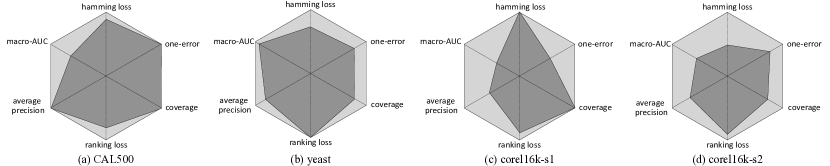
Figure 2: The performance comparison on CAL500, yeast, corel16k-s1 and corel16k-s2. The light hexagon represents the performance of MLDF, the darker one represents the performance of MLDF without the measure-aware feature reuse mechanism. The larger the area means the better performance.

4.4 Effect of measure-aware layer growth

We conduct experiments on yeast dataset to show effect of the measure-aware layer growth mechanism. Specifically, when MLDF arrives its final layer index $L$, we keep the layer increase for observing whether the mechanism is effective. The number of trees in RF-PCT is 100, and the 5-fold cross-validation is used.

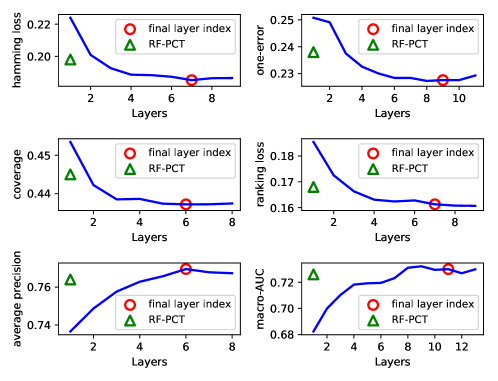
Figure 3: The test performance of MLDF in each layer on six measures on yeast dataset respectively. The triangle indicates the performance of RF-PCT, and the circle means the final layer index $L$.

Figure 3 shows the yeast’s test performance curve of MLDF on 6 measures. The red circle means the final layer returned by Algorithm 3. For RF-PCT, we set the same trees as the final layer of MLDF (the red circle). The triangle indicates the performance of RF-PCT, which can be seen as a one-layer MLDF. In Figure 3, the performance of MLDF becomes better when the model goes deeper, and our algorithm can stop almost at the position with the best performance. It demonstrates the effectiveness of our stopping mechanism. The performance of MLDF (the circle) is better than RF-PCT (the triangle), where they have the same amount of trees. Moreover, MLDF controlled by different measures can converge in different layers. It indicates that the measure-aware layer growth mechanism is effective.

4.5 Label correlations exploitation

Table 5: Predictive performance (mean $\pm$ standard deviation) of each comparing methods on all datasets. ($\cdot/\cdot/\cdot$) indicates the times that MLDF is significantly (superior/ equal/ inferior) to the comparing method on the criterion based on paired $t$-test at 95% significant level.

dataset	hamming loss	one-error	coverage	ranking loss	average precision	macro-AUC
CAL500	0.137$\pm$0.001 (5/0/0)	0.120$\pm$0.018 (4/0/1)	0.738$\pm$0.004 (5/0/0)	0.176$\pm$0.002 (5/0/0)	0.511$\pm$0.005 (4/0/1)	0.569$\pm$0.007 (5/0/0)
enron	0.047$\pm$0.001 (5/0/0)	0.225$\pm$0.007 (5/0/0)	0.224$\pm$0.005 (4/0/1)	0.079$\pm$0.004 (5/0/0)	0.691$\pm$0.003 (5/0/0)	0.738$\pm$0.005 (5/0/0)
image	0.146$\pm$0.004 (5/0/0)	0.243$\pm$0.016 (5/0/0)	0.157$\pm$0.008 (5/0/0)	0.130$\pm$0.010 (5/0/0)	0.841$\pm$0.010 (5/0/0)	0.886$\pm$0.010 (5/0/0)
scene	0.083$\pm$0.003 (5/0/0)	0.192$\pm$0.007 (5/0/0)	0.063$\pm$0.002 (5/0/0)	0.059$\pm$0.002 (5/0/0)	0.889$\pm$0.004 (5/0/0)	0.956$\pm$0.003 (5/0/0)
yeast	0.190$\pm$0.003 (5/0/0)	0.225$\pm$0.009 (5/0/0)	0.434$\pm$0.006 (5/0/0)	0.159$\pm$0.002 (5/0/0)	0.769$\pm$0.003 (5/0/0)	0.733$\pm$0.006 (5/0/0)
corel16k-s1	0.019$\pm$0.001 (5/0/0)	0.726$\pm$0.002 (2/0/3)	0.316$\pm$0.012 (5/0/0)	0.163$\pm$0.007 (4/0/1)	0.295$\pm$0.002 (4/0/1)	0.695$\pm$0.002 (3/0/2)
corel16k-s2	0.018$\pm$0.001 (5/0/0)	0.727$\pm$0.001 (1/0/4)	0.313$\pm$0.016 (4/0/1)	0.160$\pm$0.009 (3/0/2)	0.284$\pm$0.007 (2/0/3)	0.697$\pm$0.011 (3/0/2)
eurlex-sm	0.007$\pm$0.001 (5/0/0)	0.201$\pm$0.012 (5/0/0)	0.043$\pm$0.001 (5/0/0)	0.021$\pm$0.001 (5/0/0)	0.784$\pm$0.008 (4/0/1)	0.900$\pm$0.002 (4/0/1)
mediamill	0.027$\pm$0.001 (5/0/0)	0.144$\pm$0.002 (5/0/0)	0.128$\pm$0.002 (5/0/0)	0.035$\pm$0.001 (5/0/0)	0.725$\pm$0.010 (3/0/2)	0.843$\pm$0.004 (5/0/0)
sum of score	45/0/0	37/0/8	43/0/2	42/0/3	37/0/8	40/0/5

Intuitively, the cascade structure enables MLDF to utilize label correlations. Thus we conduct a distinctive approach to exploit label correlations. Our layer-wise method gradually considers more complex label correlations by utilizing the lower layer label representation in higher layer modelling. Here we deliberately delete a specific label in first layer representation, then train the second layer and check the influence of that malicious deletion. Suppose accuracy decrease on label B is observed after deleting label A, we consider the two labels are correlated. The relative normalized decrease indicates the strength of correlations and we show the result on scene dataset in Figure 4. As shown in Figure 4, label “Sunset" highly effects label “Leaf" each other, since missing one’s information will effect the performance sharply on the other label. Besides, label “Beach" is highly correlated with label “Urban” since sometimes they exist in scene dataset together [Boutell et al., 2004]. It indicates that MLDF utilizes some correlations between labels to get better performance in inner layers.

4.6 Flexibility

In previous experiments, RF-PCT and ERF-PCT are the forest blocks in MLDF, which achieve the best performance. A natural question will be is it possible to replace the forest block by other multi-label tree-based methods in MLDF, and how will the performance change? To investigate this problem, we take one RFML-C4.5 and one ERFML-C4.5 in MLDF. To ensure fairness, we keep all the other configurations same as those in Section 4.2.

Table 5 shows the result of MLDF based on RFML-C4.5. By comparing the results in Table 4, we count the times that MLDF wins/draws/loses the comparison. MLDF wins 100.0%, 82.2%, 95.6%, 93.3%, 82.2%, 88.9% among all the 45 comparisons on six evaluation measures respectively. It is clear that MLDF based on RFML-C4.5 also achieves the best performance among all compared methods. Thus, no matter based on RF-PCT or RFML-C4.5, MLDF can achieve the best performance. It indicates that MLDF has good flexibility.

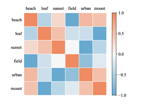
Figure 4: Effect of missing representation information on each label respectively. The scene dataset has 6 labels (top-to-down, left-to-right): “Beach", “Leaf", “Sunset", “Field", “Urban" and “Mountain".

5 CONCLUSION

In this paper, we first introduce the deep forest framework to multi-label learning and propose Multi-Label Deep Forest (MLDF). Because of the two measure-aware mechanisms, measure-aware feature reuse and measure-aware layer growth, our proposal can optimize different multi-label measures based on user demand, reduce the risk of overfitting, and achieve the best results on a bunch of benchmark datasets.

In the future, the efficiency of MLDF could be further improved by reusing some components during the process of forests training. Though our method can exploit high-order label correlations, we only show the second-order correlations in experiments. We will try to find a way to interpret how high-order correlations are used. Furthermore, we plan to embed extreme multi-label tree methods like FastXML [Prabhu and Varma, 2014] into MLDF and test the performance on extreme scale multi-label problems.

References

- Belanger et al. [2017] D. Belanger, B. Yang, and A. McCallum. End-to-End Learning for Structured Prediction Energy Networks. In ICML, pages 429–439, 2017.
- Blockeel et al. [1998] H. Blockeel, L. D. Raedt, and J. Ramon. Top-Down Induction of Clustering Trees. In ICML, pages 55–63, 1998.
- Boutell et al. [2004] M. R. Boutell, J. Luo, X. Shen, and C. M. Brown. Learning multi-label scene classification. Pattern Recognition, 37(9):1757–1771, 2004.
- Cheng et al. [2017] X. Cheng, S.-G. Zhao, X. Xuan, and K.-C. Chou. iATC-mHyb: a hybrid multi-label classifier for predicting the classification of anatomical therapeutic chemicals. Oncotarget, 8(35):58494, 2017.
- Clare and King [2001] A. Clare and R. D. King. Knowledge discovery in multi-label phenotype data. In PKDD, pages 42–53, 2001.
- Feng and Zhou [2018] J. Feng and Z.-H. Zhou. Autoencoder by Forest. In AAAI, pages 2967–2973, 2018.
- Geurts et al. [2006] P. Geurts, D. Ernst, and L. Wehenkel. Extremely randomized trees. Machine Learning, 63(1):3–42, 2006.
- Hinton and Salakhutdinov [2006] G. Hinton and R. Salakhutdinov. Reducing the dimensionality of data with neural networks. Science, 313(5786):504–507, 2006.
- Kocev and Ceci [2015] D. Kocev and M. Ceci. Ensembles of extremely randomized trees for multi-target regression. In Discovery Science, pages 86–100, 2015.
- Kocev et al. [2013] D. Kocev, C. Vens, J. Struyf, and S. Džeroski. Tree ensembles for predicting structured outputs. Pattern Recognition, 46(3):817–833, 2013.
- Madjarov et al. [2012] G. Madjarov, D. Kocev, D. Gjorgjevikj, and S. Džeroski. An extensive experimental comparison of methods for multi-label learning. Pattern Recognition, 45(9):3084–3104, 2012.
- Nam et al. [2014] J. Nam, J. Kim, E. Loza Menc’ia, I. Gurevych, and J. Fürnkranz. Large-scale multi-label text classification - revisiting neural networks. In ECML, pages 437–452, 2014.
- Pang et al. [2018] M. Pang, K.-M. Ting, P. Zhao, and Z.-H. Zhou. Improving Deep Forest by Confidence Screening. In ICDM, pages 1194–1199, 2018.
- Platt et al. [1999] J. Platt et al. Probabilistic outputs for support vector machines and comparisons to regularized likelihood methods. Advances in large margin classifiers, 10(3):61–74, 1999.
- Prabhu and Varma [2014] Y. Prabhu and M. Varma. Fastxml: A fast, accurate and stable tree-classifier for extreme multi-label learning. In KDD, pages 263–272, 2014.
- Ray et al. [2018] J. Ray, H. Wang, D. Tran, Y. Wang, M. Feiszli, L. Torresani, and M. Paluri. Scenes-Objects-Actions: A Multi-Task, Multi-Label Video Dataset. In ECCV, pages 660–676, 2018.
- Read et al. [2011] J. Read, B. Pfahringer, G. Holmes, and E. Frank. Classifier chains for multi-label classification. Machine Learning, 85(3):333–359, 2011.
- Read et al. [2016] J. Read, P. Reutemann, B. Pfahringer, and G. Holmes. MEKA: A multi-label/multi-target extension to Weka. Journal of Machine Learning Research, 17(21):1–5, 2016.
- Schapire and Singer [2000] R. E. Schapire and Y. Singer. Boostexter: A boosting-based system for text categorization. Machine learning, 39(2-3):135–168, 2000.
- Tsoumakas and Katakis [2007] G. Tsoumakas and I. Katakis. Multi-label classification: An overview. International Journal of Data Warehousing and Mining, 3(3):1–13, 2007.
- Tsoumakas and Vlahavas [2007] G. Tsoumakas and I. P. Vlahavas. Random k -labelsets: An ensemble method for multilabel classification. In ECML, pages 406–417, 2007.
- Tsoumakas et al. [2010] G. Tsoumakas, I. Katakis, and I. P. Vlahavas. Mining multi-label data. In Data Mining and Knowledge Discovery Handbook, pages 667–685. 2010.
- Wang et al. [2016] J. Wang, Y. Yang, J. Mao, Z. Huang, C. Huang, and W. Xu. CNN-RNN: A unified framework for multi-label image classification. In CVPR, pages 2285–2294, 2016.
- Wu and Zhou [2017] X.-Z. Wu and Z.-H. Zhou. A Unified View of Multi-Label Performance Measures. In ICML, pages 3780–3788, 2017.
- Zhang and Zhou [2006] M.-L. Zhang and Z.-H. Zhou. Multi-label neural networks with applications to functional genomics and text categorization. IEEE Transactions on Knowledge and Data Engineering, 18(10):1338–1351, 2006.
- Zhang and Zhou [2014] M.-L. Zhang and Z.-H. Zhou. A review on multi-label learning algorithms. IEEE Transactions on Knowledge and Data Engineering, 26(8):1819–1837, 2014.
- Zhang et al. [2018a] Q.-W. Zhang, Y. Zhong, and M.-L. Zhang. Feature-induced labeling information enrichment for multi-label learning. In AAAI, pages 4446–4453, 2018a.
- Zhang et al. [2018b] Y.-L. Zhang, J. Zhou, W. Zheng, J. Feng, L. Li, Z. Liu, M. Li, Z. Zhang, C. Chen, X. Li, and Z.-H. Zhou. Distributed Deep Forest and its Application to Automatic Detection of Cash-out Fraud. CoRR, abs/1805.04234, 2018b.
- Zhao et al. [2015] F. Zhao, Y. Huang, L. Wang, and T. Tan. Deep semantic ranking based hashing for multi-label image retrieval. In CVPR, pages 1556–1564, 2015.
- Zhou and El-Gohary [2015] P. Zhou and N. El-Gohary. Ontology-based multilabel text classification of construction regulatory documents. Journal of Computing in Civil Engineering, 30(4):04015058, 2015.
- Zhou [2012] Z.-H. Zhou. Ensemble methods: foundations and algorithms. Chapman and Hall/CRC, 2012.
- Zhou and Feng [2017] Z.-H. Zhou and J. Feng. Deep Forest: Towards An Alternative to Deep Neural Networks. In IJCAI, pages 3553–3559, 2017.
- Zhou and Feng [2018] Z.-H. Zhou and J. Feng. Deep Forest. National Science Review, page nwy108, 2018.