Feedback Linearization based on Gaussian
Processes with event-triggered Online Learning

Abstract

Combining control engineering with nonparametric modeling techniques from machine learning allows to control systems without analytic description using data-driven models. Most existing approaches separate learning, i.e. the system identification based on a fixed dataset, and control, i.e. the execution of the model-based control law. This separation makes the performance highly sensitive to the initial selection of training data and possibly requires very large datasets. This article proposes a learning feedback linearizing control law using online closed-loop identification. The employed Gaussian process model updates its training data only if the model uncertainty becomes too large. This event-triggered online learning ensures high data efficiency and thereby reduces the computational complexity, which is a major barrier for using Gaussian processes under real-time constraints. We propose safe forgetting strategies of data points to adhere to budget constraint and to further increase data-efficiency. We show asymptotic stability for the tracking error under the proposed event-triggering law and illustrate the effective identification and control in simulation.

I Introduction

Data-driven control gained high attention as costs for measuring, processing and storing data is rapidly decreasing and control engineering is increasingly applied in areas where it is difficult to describe the plant using first principles. Nevertheless, a precise system description is essential for many modern model-based control algorithms as e.g. model predictive control and feedback linearization. Classical system identification using parametric models like autoregressive moving average (ARMA) or Hammerstein models [1], reaches its limits when the choice of a suitable model class is cumbersome or impossible, e.g. in systems where human behavior is part of the control loop. That is where data-driven nonparametric models have their advantages as only minimal prior knowledge is required and allow higher flexibility than parametric models.

This article particularly considers Gaussian processes (GPs) which are well recognized in machine learning and control for modeling complex dynamics [2]. The Bayesian background allows an implicit bias-variance trade-off [3] and as GPs are a kernel based method, prior knowledge (if any exists) can properly be transferred into the model [4]. The major advantage is, that GP models also encode their own ignorance and therefore provide information whether the model is reliable for particular inputs or not.

Due to their nonparametric nature, the model complexity of a GP increases with the number of available data. This possible unlimited expressive power is generally desired, however may cause difficulties from a computational point of view in the case of large training data sets. Particularly challenging are online learning schemes where data points are accumulated over time and real-time capability is critical. This raises the question of efficient online learning strategies for nonparametric models. Time-triggered model adaptation fails to distinguish whether a new measurement or training point is necessary at the current location of the state-space or not. This calls for an event-triggered scheme, which decides upon a new measurement based on the current reliability of the model, which is expected to result in higher data-efficiency.

Figure 1: Proposed concept of an online learning control law with event-triggered model updates.

I-A Related work

The fact that no model can initially capture all aspects of the true system motivated robust and adaptive control methods to overcome this discrepancy [5]. The online adaptation of the control strategy or its employed model is well understood for parametric models [6], [7]. In particular for linear systems, data-driven approaches are extensively researched, see [8], and [9]. For nonlinear systems, model reference adaptive control (MRAC) is designed to effectively deal with model uncertainties or only little prior knowledge using online parameter estimation [10]. Iterative learning control (ILC) improves control performance by iteratively modulating the control signal in a repetitive task, such that experience from earlier executions are used to improve performance, see [11] and [12]. However, most existing MRAC and ILC methods are mainly based on parametric models which suffer from limited complexity and flexibility. Model-free adaptive control (MFAC) avoids an explicit model but instead employs e.g. a dynamic linearization [13], virtual reference feedback tuning [14] or a closed-loop control parameter optimization [15]. Alternatively, a spectral analysis for nonparametric frequency-domain tuning is considered [16] or extremum seeking is employed for performance optimization [17].

Other than in classical control theory, the machine learning literature employs more frequently data-driven models with infinite expressive power for online adaptation [18]. The class of model-based reinforcement learning algorithms considers continuous model and controller updates to maximize a reward [19]. For example [20] shows a high data efficiency with Gaussian process models. These are also successfully applied in robotics [21, 22], however most approaches miss a formal stability analysis for the system’s behavior.

Very recently, several control approaches with formal guarantees for GP models have been developed which, however, keep a fixed dataset during execution of the control law [23], [24]. The work in [25] considers the control of Lagrangian systems and shows boundedness of the tracking error. The identification of a priori known stable systems with GPs is analyzed in [26], and [27] proposes an uncertainty-based control approach for which asymptotic stability is proven. However, none of these techniques updates the model while controlling the system. The work in [28] proposes a safe exploration by sequentially adding training points to the dataset, but it only stays within the region of attraction and cannot track an arbitrary trajectory in the state space.

An online learning tracking control law with with time-triggered adaptation is proposed in [29]. As a result data points are added to the training dataset irrespectively of their importance. This might compromise real-time capability as the computational inefficiency for large datasets is a known challenge of GPs [3].

This difficulty in circumvented in [30, 31], where the unknown dynamics is estimated using high gain filters. However, these approaches suffer from the known difficulties of high gain control, i.e. a quick saturation of input signals and the amplification of noise. The latter is avoidable by combining feedback and model-based feedforward control. This idea is not just employed in this article, but was also used in [32], where a neural network identifies the dynamics without any parametric prior knowledge. Particularly [33], [34] and [35] focus on stability and performance guarantees. The work in [36] proposes a feedback linearizing control law, which adapts online the weights of a neural network model. It shows boundedness of the adaptation law and the resulting controller but cannot quantify the ultimate bound because neural networks - in comparison to GPs - do not inherently provide a measure for the fidelity of the model [37]. This becomes important, if the controller is applied in safety critical domains, where the tracking error must be quantified to avoid failure or damage to the system.

In summary, to date there exists no approach, which adapts a nonparametric model online to guarantee asymptotic stability of the tracking error. Thus for universal models, which can represent arbitrarily complex dynamics, there are missing online learning control laws, to guarantee safe behavior of the closed-loop system. Also a data-efficient update strategy is required to keep the model computationally efficient, which is important in many real-time critical applications.

I-B Contribution and structure

The main contribution of this article is an online learning feedback linearizing control law based on Gaussian processes for an initially unknown system. This control algorithm includes a closed-loop identification scheme for control affine systems exploiting compound kernels for GPs. To ensure data-efficiency of the approach, we propose an event-triggered online learning mechanism which decides upon a model update based on its current reliability. The derivation is based on a probabilistic upper bound for the model error of a GP, and allows to provide safety guarantees in terms of convergence properties of the closed-loop system. For noiseless training data, we show global asymptotic stability and for noisy output training data global ultimate boundedness of the tracking error. For the case of a constraint budget for data points, we propose a forgetting strategy, which maintains the convergence guarantees using a reduced number of training points.

The article is based on the preliminary work in [38], which focuses on the identification of a control affine system with GPs given a fixed dataset. In contrast, this work considers the online collection of data and updates the model while the control law is active. This allows to show asymptotic stability with a data-efficient event-triggered update rule while [38] only showed existence of an ultimate bound.

This article is structured as follows: After formulating the considered problem formally in Sec. II, Sec. III reviews the identification of control affine systems based on GPs. In Sec. IV, the feedback linearizing tracking control law is proposed including a convergence analysis for training data measured online at arbitrary time instances. Section V introduces an event-triggering to update the model based on its uncertainty. A numerical illustration is provided in Sec. VI followed by a conclusion in Sec. VII.

I-C Notation

Lower/upper case bold symbols denote vectors/matrices, $\mathbb{R}_{+,0}$/$\mathbb{R}_{+}$ all real positive numbers with/without zero, $\mathbb{N}_{0}$/$\mathbb{N}$ all natural numbers with/without zero, $\sigma_{\text{min}}(\cdot),\sigma_{\text{max}}(\cdot)$ the minimal/maximal singular value of a matrix and $\mathbb{E}[\cdot]$/$\mathbb{V}[\cdot]$ the expected value/variance of a random variable, respectively. $\boldsymbol{I}_{n}$ denotes the $n\times n$ identity matrix, $\mathcal{N}(\mu,\sigma)$ a Gaussian distribution with mean $\mu$ and variance $\sigma$, $\boldsymbol{a}_{1:n}$ the first $n$ elements of the vector $\boldsymbol{a}$, $\cdot\succ 0$ the positive definiteness of matrix or function and $\|\cdot\|$ the Euclidean norm if not stated otherwise.

II Problem Formulation

Consider a single-input system in the controllable canonical form

$$\dot{x}_{1} =x_{2}$$

$$\dot{x}_{2} =x_{3}$$

$$\ \cdots$$

$$\dot{x}_{n} =f(\boldsymbol{x})+g(\boldsymbol{x})u,\quad\boldsymbol{x}_{0}=\boldsymbol{x}(0),$$ (1)

with state $\boldsymbol{x}=[x_{1}\ x_{2}\cdots x_{n}]^{\intercal}\in\mathbb{X}\subseteq\mathbb{R}^{n}$ and input $u\in\mathbb{U}=\mathbb{R}$; the functions $f(\cdot)$ and $g(\cdot)$ are considered unknown. The following assumptions are made.

Assumption 1

The unknown functions $f:\mathbb{X}\to\mathbb{R}$ and $g:\mathbb{X}\to\mathbb{R}$ are globally bounded and differentiable.

Differentiability is a very natural assumption, as it holds for many physical systems. The boundedness of the functions $f(\cdot),g(\cdot)$ would automatically be implied (due to the differentiability) if the set $\mathbb{X}$ was bounded. However, we want $\mathbb{X}$ to be possibly unbounded.

From Assumption 1, the first property is derived.

Lemma 1

Consider the system (II) under Assumption 1 with bounded and continuous $u(\boldsymbol{x})$. Then the solution $\boldsymbol{x}(t)$ does not have a finite escape time, thus $\nexists t_{\infty}$, $0<t_{\infty}<\infty$ for which

$$\lim\limits_{t\to t_{\infty}}\lVert\boldsymbol{x}(t)\rVert=\infty.$$ (2)

Proof:

According to [39, Theorem 3.2] the stated conditions ensure a unique solution $\boldsymbol{x}(t)$, for all $t>0$ for which the finite escape time follows from the differentiability of $f(\cdot),g(\cdot)$ and the bounded control input. ∎

As a stabilizing controller is not known in advance (because $f(\cdot),g(\cdot)$ are unknown), the absence of a finite escape time is important: It allows to collect observations of the system in any finite time interval with a “poor” controller (or also $u(\boldsymbol{x})=0$) without risking damage due to “infinite” states. Additionally, we assume the following.

Assumption 2

For system (II) holds $g(\boldsymbol{x})>0,\mbox{$\forall\boldsymbol{x}\in\mathbb{X}$}$.

This ensures that the system’s relative degree is equal to the system order $n$ for all $\boldsymbol{x}\in\mathbb{X}$ and the sign of $g(\cdot)$ is known. Equivalently, $g(\cdot)$ can also be taken as strictly negative resulting in a change of sign for the control input. Assumption 2 is necessary to ensure global controllability and excludes the existence of internal dynamics. It restricts the system class, however the focus on this work is on the online learning control and extending it to a larger system classes is part of future work.

We assume that observations are taken online while the proposed control law is active.

Assumption 3

Noiseless measurements of the state vector $\boldsymbol{x}^{(\kappa)}=\boldsymbol{x}(t_{\kappa})$ and noisy measurements of the highest derivative $\boldsymbol{y}^{(\kappa)}=\dot{x}_{n}(t_{\kappa})+\epsilon^{(\kappa)}$ can be taken at arbitrary time instances $t_{\kappa}$ with $\kappa\in\mathbb{N}_{0}$. The observation noise $\epsilon^{(\kappa)}\sim\mathcal{N}(0,\sigma_{\text{on}}^{2})$ is assumed Gaussian, independent and identically distributed. The time-varying dataset

$$\mathbb{D}_{\kappa}=\left\{\boldsymbol{x}^{(i)},y^{(i)}\right\}_{i=1}^{N_{\kappa}},$$ (3)

is updated at time $t_{\kappa}$ and remains constant until $t_{\kappa+1}$ and $N_{\kappa}\in\mathbb{N}_{0}$ denotes the current number of data points.

The exact measurement of the state is a common assumption and necessary for feedback linearization. The time derivative of the state $x_{n}$ can, for practical applications, be approximated through finite differences. The approximation error is then considered as part of the measurement noise as other additive sources of imprecision result in an overall sub-Gaussian noise distribution. Alternatively, a separate sensor for measurements of $\dot{x}_{n}$ is necessary.

Throughout this article, we will refer to $\sigma_{\text{on}}^{2}=0$ as the noiseless case and $\sigma_{\text{on}}^{2}>0$ as the noisy case considering measurements of $\dot{x}_{n}$. The measurement of the state $\boldsymbol{x}$ will always be assumed noise free.

Consider, that $N_{\kappa}$ is not necessarily increasing with increasing $\kappa$ as data pairs can also be discarded from the dataset if not needed anymore. However, this set $\mathbb{D}_{\kappa}$ remains constant between two consecutive measurements, because elements are only added or removed at $t_{\kappa}$.

The goal is to design an online learning feedback linearizing control law - based on dataset $\mathbb{D}_{\kappa}$ - of the form

$$u_{\kappa}(\boldsymbol{x})=\frac{1}{\hat{g}_{\kappa}(\boldsymbol{x})}\left(-\hat{f}_{\kappa}(\boldsymbol{x})+\nu\right),\quad\kappa\in\mathbb{N}_{0},$$ (4)

where $\nu\in\mathbb{R}$ is the input to the resulting approximately linearized system and the functions $\hat{f}_{\kappa}:\mathbb{X}\to\mathbb{R}$, $\hat{g}_{\kappa}:\mathbb{X}\to\mathbb{R}$ are the approximations for the unknown functions $f(\boldsymbol{x})$, $g(\boldsymbol{x})$. The control law (4) is switching, because the model $\hat{f}_{\kappa}(\boldsymbol{x})$, $\hat{g}_{\kappa}(\boldsymbol{x})$ is updated with every change of the dataset $\mathbb{D}_{\kappa}$ at time $t_{\kappa}$. We would like to emphasize, that measurements are not taken at a constant time interval, and updates are therefore not performed periodically. Instead, the updates will be performed when needed, i.e. triggered by an event (introduced in Sec. V) and thus $t_{\kappa}$ for $\kappa\in\mathbb{N}_{0}$ are not equidistant. By definition, the $\kappa$-th update occurs at $t_{\kappa}$ and the control law $u_{\kappa}$ is then applied until the next event at $t_{\kappa+1}$, more formally written as

$$u(\boldsymbol{x})=u_{\kappa}(\boldsymbol{x}),\quad t\in[t_{\kappa}\ t_{\kappa+1}).$$ (5)

III Gaussian Process Learning for Control Affine Systems

For the closed-loop online identification of $f(\cdot)$ and $g(\cdot)$ we consider Gaussian process regression, which then provides the approximations $\hat{f}_{\kappa}(\cdot)$ and $\hat{g}_{\kappa}(\cdot)$. We will first introduce GP regression in general (Sec. III-A), before presenting our tailored solution for control affine closed-loop systems in Sec. III-B.

III-A Gaussian process regression

Consider a function $f_{\text{true}}\colon\mathbb{X}\to\mathbb{R}$ for which noisy measurements of the image at the locations $\boldsymbol{x}^{(i)}\in\mathbb{X}$ are available, thus

$$y_{f}^{(i)}=f_{\text{true}}\left(\boldsymbol{x}^{(i)}\right)+\epsilon^{(i)},$$ (6)

where $\epsilon^{(i)}\sim\mathcal{N}(0,\sigma_{\text{on}}^{2})$ and $i=1,\ldots,N$ (where we write simply $N$ for $N_{\kappa}$ in this section). Modeling this function with a Gaussian process $f_{\mathcal{GP}}(\boldsymbol{x})$ results in a stochastic process which assigns a Gaussian distribution to any finite subset $\{\boldsymbol{x}_{1},\ldots,\boldsymbol{x}_{M}\}\subset\mathbb{X}$ in a continuous domain. The GP is also often considered as distribution over functions [3], denoted by

$$f_{\mathcal{GP}}(\boldsymbol{x})\sim\mathcal{GP}\left(m(\boldsymbol{x}),k(\boldsymbol{x},\boldsymbol{x}^{\prime})\right),$$ (7)

and is fully specified by a mean $m(\boldsymbol{x}):\mathbb{X}\to\mathbb{R}$ and covariance $k(\boldsymbol{x},\boldsymbol{x}^{\prime}):\mathbb{X}\times\mathbb{X}\to\mathbb{R}$ function. The mean function includes prior knowledge of the function $f_{\text{true}}$ if there is any. Otherwise, it is commonly set to zero. The covariance function, also called kernel function, determines properties of $f_{\mathcal{GP}}(\boldsymbol{x})$, like the smoothness and signal variance. Mean and kernel function are described by the hyperparameters $\boldsymbol{\psi}$.

Using Bayesian techniques, the likelihood function

$$\boldsymbol{\psi}^{*} =\arg\max\limits_{\boldsymbol{\psi}}\log p(\boldsymbol{y}_{f}|\boldsymbol{X},\boldsymbol{\psi}),$$ (8)

$$\log p(\boldsymbol{y}_{f}|\boldsymbol{X},\boldsymbol{\psi}) =\frac{1}{2}\left(\boldsymbol{y}_{f}^{T}\boldsymbol{K}^{-1}\boldsymbol{y}_{f}-\log\det\boldsymbol{K}-N\log(2\pi)\right),$$

is maximized to obtain the optimal hyperparameters for a given set of observations. As notation we use

$$\boldsymbol{X} =\left[\boldsymbol{x}^{(1)}\ \cdots\ \boldsymbol{x}^{(N)}\right]\in\mathbb{R}^{n\times N},$$ (9)

$$\boldsymbol{y}_{f} =\left[y_{f}^{(1)}\ \cdots\ y_{f}^{(N)}\right]^{\intercal}\in\mathbb{R}^{N},$$ (10)

to denote the input/output data, respectively and

$$\boldsymbol{K} \!=\!\begin{bmatrix}k\left(\boldsymbol{x}^{(1)},\boldsymbol{x}^{(1)}\right)&\!\cdots\!&k\left(\boldsymbol{x}^{(1)},\boldsymbol{x}^{(N)}\right)\\ \vdots&\!\ddots\!&\vdots\\ k\left(\boldsymbol{x}^{(N)},\boldsymbol{x}^{(1)}\right)&\!\cdots\!&k\left(\boldsymbol{x}^{(N)},\boldsymbol{x}^{(N)}\right)\end{bmatrix}\!\in\!\mathbb{R}^{N\times N}$$ (11)

concatenates kernel evaluations of pairs of input data. Although the optimization (8) is generally non-convex, it is usually performed with conjugated gradient-based methods [3]. Each local minimum can be considered as a different interpretation of data and we discuss the effect of suboptimal identification in Sec. III-C.

In a regression task, GPs employ the joint Gaussian distribution of training data $\boldsymbol{X},\boldsymbol{y}_{f}$ and a test input $\boldsymbol{x}^{*}$

$$\begin{bmatrix}f_{\mathcal{GP}}(\boldsymbol{x}^{*})\\ \boldsymbol{y}_{f}\end{bmatrix}\sim\mathcal{N}\left(\begin{bmatrix}m(\boldsymbol{x}^{*})\\ \boldsymbol{m}^{\boldsymbol{X}}\end{bmatrix},\begin{bmatrix}k^{*}&\boldsymbol{k}^{\intercal}\\ \boldsymbol{k}&\boldsymbol{K}+\sigma_{\text{on}}^{2}\boldsymbol{I}_{N}\end{bmatrix}\right),$$ (12)

where

$$\boldsymbol{m}^{\boldsymbol{X}}=\begin{bmatrix}m\left(\boldsymbol{x}^{(1)}\right)&\cdots&m\left(\boldsymbol{x}^{(N)}\right)\end{bmatrix}^{\intercal},$$ (13)

to find the posterior mean and variance function

$$\mu(\boldsymbol{x}^{*}) :=\mathbb{E}\left[f_{\mathcal{GP}}(\boldsymbol{x}^{*})|\boldsymbol{X},\boldsymbol{y}_{f}\right]$$ (14)

$$\ =m(\boldsymbol{x}^{*})+\boldsymbol{k}^{\intercal}(\boldsymbol{K}+\sigma_{\text{on}}^{2}\boldsymbol{I}_{N})^{-1}(\boldsymbol{y}_{f}-\boldsymbol{m}^{\boldsymbol{X}}),$$

$$\sigma(\boldsymbol{x}^{*}) :=\mathbb{V}\left[f_{\mathcal{GP}}(\boldsymbol{x}^{*})\right|\boldsymbol{X},\boldsymbol{y}_{f}]$$ (15)

$$\ =k^{*}-\boldsymbol{k}^{\intercal}(\boldsymbol{K}+\sigma_{\text{on}}^{2}\boldsymbol{I}_{N})^{-1}\boldsymbol{k},$$

through conditioning, where

$$\begin{aligned} k^{*}&=k(\boldsymbol{x}^{*},\boldsymbol{x}^{*}),\\ \boldsymbol{k}&=\left[k\left(\boldsymbol{x}^{(1)},\boldsymbol{x}^{*}\right)\ \cdots\ k\left(\boldsymbol{x}^{(N)},\boldsymbol{x}^{*}\right)\right]^{\intercal}\in\mathbb{R}^{N}.\end{aligned}$$ (16)

However, considering the defined problem in Sec. II, the classical GP regression framework cannot be directly applied, because closed-loop measurements do not provide data points for $f(\cdot)$ and $g(\cdot)$ separately. Therefore, the following section explains how it is augmented using the given prior knowledge.

III-B Closed-loop identification with prior knowledge

First, we transfer the knowledge on the positivity of the function $g(\boldsymbol{x})$ from Assumption 2 into the model $\hat{g}(\boldsymbol{x})$. It is crucial to utilize this knowledge for the model to ensure the feedback linearizing control (4) results in well behaved control signals. Using a GP model for $\hat{g}(\boldsymbol{x})$, this can be ensured using a proper prior mean function.

Lemma 2

Consider the posterior mean function (14) with a bounded and differentiable kernel $k(\cdot,\cdot)$ and a dataset $(\boldsymbol{X},\boldsymbol{y}_{f})$ for which $\boldsymbol{x}^{(i)}\neq\boldsymbol{x}^{(i^{\prime})}$ and $y^{(i)}_{f}>0$, hold $\forall i,i^{\prime}=1,\ldots,N,i\neq i^{\prime}$. Then, there exists a differentiable prior mean function $m(\boldsymbol{x})$ such that

$$\mu(\boldsymbol{x})>0,\qquad\mbox{$\forall\boldsymbol{x}\in\mathbb{X}$}.$$ (17)

Proof:

Consider a prior mean function for which holds $0<m\left(\boldsymbol{x}^{(i)}\right)<\infty$, $\forall\mbox{$i=1,\ldots,N$ }$, then, a differentiable $m(\boldsymbol{x})$ can $\forall\boldsymbol{x}\in\mathbb{X}\setminus\left\{\boldsymbol{x}^{(1)},\ldots,\boldsymbol{x}^{(N)}\right\}$ always be chosen larger than the constant $\boldsymbol{k}^{\intercal}(\boldsymbol{K}+\sigma_{\text{on}}^{2}\boldsymbol{I}_{N})^{-1}\left(\boldsymbol{y}_{f}-\boldsymbol{m}^{\boldsymbol{X}}\right)$, because the latter is bounded. For $\boldsymbol{x}\in\left\{\boldsymbol{x}^{(1)},\ldots,\boldsymbol{x}^{(N)}\right\}$ a choice $m\left(\boldsymbol{x}^{(i)}\right)=y^{(i)}_{f}$ (which complies with the first condition) ensures, that $\mu(\boldsymbol{x})$ is strictly positive. ∎

Remark 1

Since $g(\cdot)$ is strictly positive by Assumption 2, the condition $y^{(i)}_{f}>0$ follows naturally. In case the Gaussian noise results in negative measurements $y^{(i)}$, it can be corrected using $\max(y^{(i)},\eta)$, with an arbitrarily small $\eta>0$. Alternatively, strictly positive noise distributions, e.g. a Gamma distribution can also be combined with Gaussian process regression [3].

In practice, it is often sufficient to set $m(\boldsymbol{x})$ to a positive constant. To verify that $\mu(\boldsymbol{x})>0$ holds, the techniques in [28] can be utilized. The suitable prior mean function according to Lemma 2 will be denoted by $m_{g}(\boldsymbol{x})$.

Second, the major difficulty of closed-loop identification is to differentiate the effect of the control input and the unforced dynamics. For the control affine structure, this means that individual measurements of the functions $f(\cdot)$ and $g(\cdot)$ from (II) are not provided. Thus, functions $f(\cdot),g(\cdot)$ must be identified from only observing their sum exploiting the control affine structure. We propose to utilize a compound kernels as reviewed in Appendix A based on [4]. More specifically, we use the composite kernel

$$k(\boldsymbol{x},\boldsymbol{x}^{\prime})=k_{f}(\boldsymbol{x},\boldsymbol{x}^{\prime})+u(\boldsymbol{x})k_{g}(\boldsymbol{x},\boldsymbol{x}^{\prime})u(\boldsymbol{x}^{\prime}),$$ (18)

which replicates the structure of a control affine system: the first summand $k_{f}(\cdot,\cdot)$ represents the unknown unforced dynamics $f(\cdot)$; the second summand $u(\cdot)k_{g}(\cdot,\cdot)u(\cdot)$ the product of the unknown scaling of the control $g(\cdot)$ and the known state feedback control term $u(\cdot)$. As no further knowledge regarding $f(\cdot),g(\cdot)$ is given, we employ two squared exponential (SE) kernels with automatic relevance determination

$$k_{f}(\boldsymbol{x},\boldsymbol{x}^{\prime}) =\sigma_{f}^{2}\exp\left(\sum_{j=1}^{n}\frac{(x_{j}-x^{\prime}_{j})^{2}}{-2l_{j,f}^{2}}\right),$$ (19)

$$k_{g}(\boldsymbol{x},\boldsymbol{x}^{\prime}) =\sigma_{g}^{2}\exp\left(\sum_{j=1}^{n}\frac{(x_{j}-x^{\prime}_{j})^{2}}{-2l_{j,g}^{2}}\right),$$ (20)

where the hyperparameters are the lengthscales $l_{j,f},l_{j,g}\!\in\!\mathbb{R}_{+}$, $j=1,\ldots,n$ and the signal variances $\sigma_{f},\sigma_{g}\in\mathbb{R}_{+}^{0}$. For notational convenience, they are concatenated in the vector

$$\boldsymbol{\psi}_{gf}=\left[l_{1,f}\ l_{1,g}\ \cdots\ l_{n,f}\ l_{n,g}\ \sigma_{f}^{2}\ \sigma_{g}^{2}\right]^{\intercal}.$$ (21)

The SE kernel is universal and therefore allows to model any continuous function arbitrarily exactly according to [40].

Remark 2

GP models with structured kernels, like (18), must not be confused with parametric models, which have a predetermined structure and use a fixed number of parameters. In contrast a GP with a structured kernel has potentially infinitely many parameters for each part of its structure. So the kernel encodes the knowledge, that the unknown function e.g. is build of a sum, but each summand has unlimited flexibility.

We denote $\boldsymbol{U}=\text{diag}\left(u_{1}\left(\boldsymbol{x}^{(1)}\right),\dots,u_{N}\left(\boldsymbol{x}^{(N)}\right)\right)\in\mathbb{R}^{N\times N}$, where $u_{i}$ denotes the control law which was active at the time at which the pair $\left\{\boldsymbol{x}^{(i)},y^{(i)}\right\}$ was collected for $i=1,\ldots,N$ . Furthermore, $\boldsymbol{m}_{g}^{\boldsymbol{X}}$, $\boldsymbol{y}$ are analogously defined to (13), (10), respectively. Then

$$\boldsymbol{K}_{fg}=\boldsymbol{K}_{f}+\boldsymbol{U}^{\intercal}\boldsymbol{K}_{g}\boldsymbol{U}+\sigma_{\text{on}}^{2}\boldsymbol{I}_{n},$$ (22)

and $\boldsymbol{k}_{f},\boldsymbol{k}_{g},\boldsymbol{K}_{f},\boldsymbol{K}_{g}$ are defined analogously to (16) and (11) using $k_{f}(\boldsymbol{x},\boldsymbol{x}^{\prime}),k_{g}(\boldsymbol{x},\boldsymbol{x}^{\prime})$. This notation allows to formulate the estimates $\hat{f}(\boldsymbol{x}),\hat{g}(\boldsymbol{x})$.

Lemma 3

The GP posterior mean prediction for the functions $f(\boldsymbol{x}),g(\boldsymbol{x})$, based on the training data $\mathbb{D}_{\kappa}$ in (3) for the compound kernel (18) are given by

$$\hat{f}(\boldsymbol{x}):=\mu_{f}(\boldsymbol{x}) =\boldsymbol{k}_{f}^{\intercal}\boldsymbol{K}_{fg}^{-1}\left(\boldsymbol{y}-\boldsymbol{U}\boldsymbol{m}_{g}^{\boldsymbol{X}}\right),$$ (23)

$$\hat{g}(\boldsymbol{x}):=\mu_{g}(\boldsymbol{x}) =m_{g}(\boldsymbol{x})+\boldsymbol{k}_{g}^{\intercal}\boldsymbol{U}\boldsymbol{K}_{fg}^{-1}\left(\boldsymbol{y}-\boldsymbol{U}\boldsymbol{m}_{g}^{\boldsymbol{X}}\right),$$ (24)

where the prior mean function for $\hat{f}(\boldsymbol{x})$ is set to zero, $m_{f}(\boldsymbol{x})=0$, and for $\hat{g}(\boldsymbol{x})$, $m_{g}(\boldsymbol{x})$ is chosen according to Lemma 2.

Proof:

For an input $\boldsymbol{x}$ and the compound kernel (18), the joint distribution is given by

$$\begin{bmatrix}f(\boldsymbol{x})\\ g(\boldsymbol{x})\\ \boldsymbol{y}\end{bmatrix}\!\sim\mathcal{N}\left(\begin{bmatrix}0\\ m_{g}(\boldsymbol{x})\\ \boldsymbol{U}\boldsymbol{m}_{g}^{\boldsymbol{X}}\end{bmatrix},\begin{bmatrix}k_{f}^{*}&0&\boldsymbol{k}_{f}^{\intercal}\\ 0&k_{g}^{*}&\boldsymbol{k}_{g}^{\intercal}\boldsymbol{U}^{\intercal}\\ \boldsymbol{k}_{f}&\boldsymbol{U}\boldsymbol{k}_{g}&\boldsymbol{K}_{fg}\end{bmatrix}\right)\!,$$ (25)

similarly to (12). According to [4], the posterior mean functions (23) and (24) follow equivalently to (14). ∎

For these estimates, it can be shown that all prior knowledge is properly transferred into the model.

Proposition 1

Consider a control affine system (II) under Assumptions 1, 2 and 3 and the compound kernel (18). Then, the estimates $\hat{f}(\boldsymbol{x})$ and $\hat{g}(\boldsymbol{x})$ in Lemma 3 are bounded, infinitely differentiable and there exists a prior mean function $m_{g}(\boldsymbol{x})$ and a hyperparameter vector $\boldsymbol{\psi}_{gf}$ such that $\hat{g}(\boldsymbol{x})>0$ holds $\forall\boldsymbol{x}\in\mathbb{X}$.

Proof:

The SE kernel inherits its properties differentiability and boundedness to all functions represented by the GP [3], thus also to the posterior mean functions, which are used as estimates. The strict positivity of $\hat{g}(\boldsymbol{x})$ follows from the fact, that $\sigma_{g}^{2}$ can be made arbitrarily small such that there always exists a positive function $m_{g}$, such that $m_{g}(\boldsymbol{x})$ dominates the term $\boldsymbol{k}_{g}^{\intercal}\boldsymbol{U}\boldsymbol{K}_{fg}^{-1}\left(\boldsymbol{y}-\boldsymbol{U}\boldsymbol{m}_{g}^{\boldsymbol{X}}\right)$ in (24). ∎

Remark 3

The only properties of the SE kernel which are used for the derivations and proofs are its differentiability and its boundedness. Thus, the conclusions can directly be extended to other kernel function fulfilling these properties. For the sake of focus, in this article we will consider the SE kernel only.

III-C Discussion

The most obvious challenge of the closed-loop identification is, that there exists not a unique, but infinitely many solutions for two differentiable functions to add up to the same values. Thus, only observing the sum in (II) is not promising to learn the unique correct individual functions $f(\cdot)$, $g(\cdot)$ because it is an under-determined problem. The estimates in (23) and (24) are just one of many solutions, determined by the choice of hyperparameters, which suits the training data. Nevertheless, the optimization (8) interprets the observed data to match the kernel structure, which is shown to be successful in the simulation in Sec. VI-A. For the case that the results are not satisfactory, we provide an extension in Appendix B to address this challenge. It merges data points of the closed-loop system with measurements from the temporary open-loop system. It thereby uses Lemma 1, which allows to safely turn off the control signal ($u=0$) for a finite time period. Nevertheless, we want to highlight, that the formal guarantees provided in the following section (Theorem 1) hold independently whether this extension is utilized or not.

Furthermore, additional knowledge like periodicity or dependence of $f(\cdot)$ or $g(\cdot)$ on only a subset of the state variables, can also be transferred into the kernel to facilitate the identification by using a periodic kernel or setting the lengthscales $l_{j,f}=l_{j^{\prime},g}=\infty$ for the states $j,j^{\prime}$ of which they are independent, respectively. The latter simplifies the optimization of hyperparameters as the search space is reduced. A systematic way of constructing more evolved kernel function (including more prior knowledge) is discussed in [4].

Considering the computational load, the inverse of $\boldsymbol{K}_{fg}$ is most critical, as the number of operations increases cubical with the number of data points, thus $\mathcal{O}(N^{3})$. However, adding further data points is necessary to ensure the model is precise at the current position in the state space, where the most recent data points are taken from measurements. Comparing to previous approaches, e.g. [38], where $\boldsymbol{K}_{fg}^{-1}\boldsymbol{y}$ is constant and can thereby be precomputed offline, here it must be recomputed with every update of the model as data points are added one at a time. This difficulty can be addressed using a rank-$1$ update of the inverse with the Sherman–Morrison formula [41] resulting in only  $\mathcal{O}(N^{2})$ operations. However, this quadratic computational complexity might still be very time consuming, and therefore motivates the data-efficient event-triggered model updates introduced in Sec. V.

Generally, Gaussian processes turn out to be very effective for the adaptive model control law: They properly transfer all prior assumptions consistently into the model (Proposition 1) and allow for the identification in closed-loop. The nonparametric nature allows an unlimited model flexibility and the complexity increases as more data is available in a data-driven fashion. This is a crucial advantage compared to classical system identification methods, particularly for highly nonlinear systems.

IV Feedback Linearizing Control Law

In this section, the feedback linearizing online learning control law is proposed and the resulting closed-loop behavior is analyzed. After showing ultimate boundedness for the most general case, we make further specific assumptions to provide stronger stability results. Here, further properties of the Gaussian process modeling technique is exploited: As the model error of the GP can be bounded and quantified, the ultimate bound of the tracking error can also be quantified.

Classical model reference adaptive control modifies the model parameters continuously over time, which is not possible here due to the nonparametric nature of the GP model. Thus, particular attention must be drawn to the resulting switching character of the control law, which stems from the time-varying dataset $\mathbb{D}_{\kappa}$ of the Gaussian process introduced in Assumption 3.

We are interested in tracking desired trajectories for the state $x_{1}$, given by $x_{d}(t)$, with the following property.

Assumption 4

The desired trajectory $x_{d}(t)$ is bounded and at least $n-1$ times differentiable, thus

$$\boldsymbol{x}_{d}(t)=\begin{bmatrix}x_{d}&\dot{x}_{d}&\cdots&\frac{d^{n-1}x_{d}}{dt^{n-1}}\end{bmatrix}^{\intercal}$$ (26)

is continuous and $\frac{d^{n}x_{d}}{dt^{n}}$ is bounded.

For notational convenience, we define the tracking error

$$\boldsymbol{e}=\boldsymbol{x}-\boldsymbol{x}_{d}.$$ (27)

IV-A Control law

Consider the filtered scalar state $r\in\mathbb{R}$, defined as

$$r=\begin{bmatrix}\boldsymbol{\lambda}^{\intercal}&1\end{bmatrix}\boldsymbol{e},$$ (28)

where $\boldsymbol{\lambda}=[\lambda_{1}\ \lambda_{2}\cdots\lambda_{n-1}]^{\intercal}\in\mathbb{R}^{n-1}$ is a coefficient vector such that for $s\in\mathbb{C}$ the polynomial $s^{n-1}+\lambda_{n-1}s^{n-2}+\cdots+\lambda_{1}$ is Hurwitz. Under this condition, the error converges exponentially $\boldsymbol{e}\to\boldsymbol{0}$ as $r\to 0$ [36]. The dynamics of the filtered state is

$$\dot{r}=f(\boldsymbol{x})+g(\boldsymbol{x})u(\boldsymbol{x})+\rho,$$ (29)

where

$$\rho=\boldsymbol{\lambda}^{\intercal}\boldsymbol{e}_{2:n}-\frac{d^{n}x_{d}}{dt^{n}},$$ (30)

with $\boldsymbol{e}_{2:n}=\left[e_{2}\cdots e_{n}\right]^{\intercal}\in\mathbb{R}^{n-1}$. For the control law $u(\boldsymbol{x})$, we propose

$$u_{\kappa}(\boldsymbol{x})=\frac{1}{\hat{g}_{\kappa}(\boldsymbol{x})}\left(-\hat{f}_{\kappa}(\boldsymbol{x})-k_{c}r-\rho\right),$$ (31)

according to (4) where $\nu=-k_{c}r-\rho$ with $k_{c}\in\mathbb{R}_{+}$ is used. The subscript $\kappa\in\mathbb{N}_{0}$ indicates the $\kappa$-th time interval $t\in[t_{\kappa}\ t_{\kappa+1})$ for which $u_{\kappa}$ is applied according to (5). The estimates $\hat{g}_{\kappa}(\cdot)$, $\hat{f}_{\kappa}(\cdot)$ are based on $N_{\kappa}$ training points in the time-varying dataset $\mathbb{D}_{\kappa}$ introduced in Assumption 3. The control scheme is visualized in Fig. 2 and the adaptation procedure is provided in Algorithm 1.

Note, that even though GPs itself are probabilistic models, the control law is deterministic, because it only employs the posterior mean functions as model estimate $\hat{g}_{\kappa}(\cdot)$, $\hat{f}_{\kappa}(\cdot)$.

1:initialize $\kappa=0$, $\mathbb{D}_{0}=\{\}$, $\hat{f}_{0}=0$, $\hat{g}_{0}=m_{g}(\cdot)$

2:while simulation time not exceeded do

3:     while $t<t_{\kappa+1}$ do

4:         run controller $u_{\kappa}$ in (31)

5:     end while

6:     set $\kappa\leftarrow\kappa+1$

7:     measure $\boldsymbol{x}^{(\kappa)}=\boldsymbol{x}(t_{\kappa})$ and $y^{(\kappa)}=\dot{x}_{n}(t_{\kappa})+\epsilon^{(\kappa)}$

8:     add training point $\mathbb{D}_{\kappa}=\mathbb{D}_{\kappa-1}\cup\left\{\left(\boldsymbol{x}^{(\kappa)},y^{(\kappa)}\right)\right\}$

9:     update the estimates $\hat{f}_{\kappa}(\cdot),\hat{g}_{\kappa}(\cdot)$ in (23), (24)

10:end while

Algorithm 1 Online leaning for feedback linearization control

Figure 2: The online leaning feedback linearizing control scheme including the event trigger proposed in Sec. V, which controls the switching time $t_{\kappa+1}$.

IV-B Convergence analysis

An offline version of the control law (31), with constant dataset $\mathbb{D}$ and estimates $\hat{f}(\boldsymbol{x}),\hat{g}(\boldsymbol{x})$ was introduced previously and was shown to be globally uniformly ultimately bounded [38, Proposition 1].

But, with the time-varying dataset and model, Algorithm 1 describes a switching control law. This switching results in a hybrid system, where some states are changing continuously in time but the system dynamics (or other states) change at discrete time instances. Here, the resulting closed-loop system is subject to (in general) arbitrary switching. Its convergence behavior is analyzed here based on the principle of a common Lyapunov function. It states, that a Lyapunov function, which is independent of the switching signal must decrease over time along the system’s trajectories. This is shown in the following.

Theorem 1

Consider the system (II) and a desired trajectory $\boldsymbol{x}_{d}(t)$ under Assumptions 1, 3, 2 and 4. Further consider the control law (31), where $f(\cdot),g(\cdot)$ are modeled by GP mean functions $\hat{f}_{\kappa}(\cdot),\hat{g}_{\kappa}(\cdot)$ in (23) and  (24), respectively. The GP model is updated at arbitrary switching times $t_{\kappa}$ according to Algorithm 1. Then, there exists a $k_{c}^{*}>0$ such that for every $k_{c}\geq k_{c}^{*}$ the tracking error $\left\lVert\boldsymbol{e}\right\rVert$ is globally uniformly ultimately bounded.

Proof:

Consider the common Lyapunov function candidate

$$V_{\kappa}(\boldsymbol{x})=r^{2}/2,\qquad\forall\kappa\in\mathbb{N}_{0},$$ (32)

with time derivative

$$\dot{V}_{\kappa}(\boldsymbol{x}) =r\dot{r}=r\left(f+gu_{\kappa}+\rho\right)$$ (33)

$$=r\left(f+\frac{g}{\hat{g}_{\kappa}}(-\hat{f}_{\kappa}-k_{c}r-\rho)+\rho\right)$$

$$=r\left(f-\bar{g}_{\kappa}\hat{f}_{\kappa}\right)-k_{c}\bar{g}_{\kappa}r^{2}+(1-\bar{g}_{\kappa})r\rho,$$

where $\bar{g}_{\kappa}:=\frac{g(\boldsymbol{x})}{\hat{g}_{\kappa}(\boldsymbol{x})}$ is positive and bounded $\forall\kappa$ and $\forall\boldsymbol{x}\in\mathbb{X}$ from Proposition 1 and Assumptions 1 and 2. As a consequence $\left(f-\bar{g}_{\kappa}\hat{f}_{\kappa}\right)$ is bounded and there exists a constant $\boldsymbol{a}\in\mathbb{R}^{n}$ such that

$$\left\lVert r\left(f-\bar{g}_{\kappa}\hat{f}_{\kappa}\right)\right\rVert\leq\left\lVert\boldsymbol{a}^{\intercal}\boldsymbol{e}\right\rVert\qquad\forall\boldsymbol{e},\kappa$$ (34)

holds, because $r$ only grows linearly in $\boldsymbol{e}$. For similar reasons, we can find constants $\boldsymbol{c}\in\mathbb{R}^{n}$ and $\boldsymbol{B},\boldsymbol{C}\in\mathbb{R}^{n\times n}$, with $\boldsymbol{B},\boldsymbol{C}\succ 0$ for which

$$\left\lVert\bar{g}_{\kappa}r^{2}\right\rVert \geq\boldsymbol{e}^{\intercal}\boldsymbol{B}\boldsymbol{e}, \forall\boldsymbol{e},\kappa$$ (35)

$$\left\lVert(1-\bar{g}_{\kappa})r\rho\right\rVert \leq\boldsymbol{e}^{\intercal}\boldsymbol{C}\boldsymbol{e}+\boldsymbol{c}^{\intercal}\boldsymbol{e}, \forall\boldsymbol{e},\kappa$$ (36)

holds which exist since $f,\hat{f}_{\kappa},\bar{g}_{\kappa}$ are bounded. Therefore,

$$\dot{V}_{\kappa}(\boldsymbol{x}) \leq\!\left\lVert\boldsymbol{a}\right\rVert\left\lVert\boldsymbol{e}\right\rVert\!-\!k_{c}\sigma_{\text{min}}(\boldsymbol{B})\left\lVert\boldsymbol{e}\right\rVert^{2}\!+\!\sigma_{\text{max}}(\boldsymbol{C})\left\lVert\boldsymbol{e}\right\rVert^{2}\!+\!\left\lVert\boldsymbol{c}\right\rVert\left\lVert\boldsymbol{e}\right\rVert$$

$$=\!\left\lVert\boldsymbol{e}\right\rVert\!\left(\left\lVert\boldsymbol{a}\right\rVert\!+\!\left\lVert\boldsymbol{c}\right\rVert\right)\!+\!\left\lVert\boldsymbol{e}\right\rVert^{2}\!\left(\sigma_{\text{max}}(\boldsymbol{C})\!-\!k_{c}\sigma_{\text{min}}(\boldsymbol{B})\right)$$ (37)

holds for all $\kappa$ and there exists a $k_{c}^{*}>0$ such that

$$\sigma_{\text{max}}(\boldsymbol{C})-k_{c}^{*}\sigma_{\text{min}}(\boldsymbol{B})<0.$$ (38)

As a result, for every $k_{c}\geq k_{c}^{*}$, the Lyapunov function decreases

$$\dot{V}_{\kappa}(\boldsymbol{x})<0,\qquad\mbox{$\forall\boldsymbol{x}\in\mathbb{X}$}\!\setminus\!\mathbb{B},\ \forall\kappa$$ (39)

outside of the set

$$\mathbb{B}=\left\{\mbox{$\forall\boldsymbol{x}\in\mathbb{X}$}\left|\left\lVert\boldsymbol{e}\right\rVert\leq\frac{\left\lVert\boldsymbol{a}\right\rVert+\left\lVert\boldsymbol{c}\right\rVert}{k_{c}\sigma_{\text{min}}(\boldsymbol{A})-\sigma_{\text{max}}(\boldsymbol{B})}\right.\right\},$$ (40)

which forms a tube in $\boldsymbol{x}$ coordinates around the desired trajectory and a ball in $\boldsymbol{e}$ coordinates. Thus, we have found a common radially unbounded Lyapunov function $V(\boldsymbol{x})$, which decreases $\forall\kappa$ outside of the ball $\mathbb{B}$. According to [42, Theorem 2.1], this allows the conclusion that for arbitrary switching sequences the tracking error converges to the ball $\mathbb{B}$. Since $\mathbb{B}$ is independent of the initial state, global uniform ultimate boundedness (GUUB) holds. ∎

Thus, we have shown, that the tracking error is bounded by the proposed online learning control scheme for a large enough gain $k_{c}$ with an arbitrary switching sequence. However, without further knowledge, a value for the critical gain $k_{c}^{*}$ cannot be computed. We therefore make the following simplifying assumption

Assumption 5

The function $g(\boldsymbol{x})$ is known, thus $\hat{g}(\boldsymbol{x})=g(\boldsymbol{x})$ and noisy training data observations of $\dot{x}_{n}$

$$y_{f}^{(i)}=f\left(\boldsymbol{x}^{(i)}\right)+\epsilon^{(i)}=\dot{x}_{n}^{(i)}-g\left(\boldsymbol{x}^{(i)}\right)u_{\kappa}\left(\boldsymbol{x}^{(i)}\right)+\epsilon^{(i)}$$ (41)

with $\epsilon^{(i)}\sim\mathcal{N}(0,\sigma_{\text{on}}^{2}),\ i=1,\ldots,N_{\kappa}$ are available.

This assumption holds for many real-world system, e.g. most Lagrangian systems, which is a considerably large class [43]. It is also a quite common assumption when working with control affine systems [44].

Analogously to (23), the unknown function is now estimated by

$$\hat{f}(\boldsymbol{x}):=\mu_{f}(\boldsymbol{x})=\boldsymbol{k}_{f}^{\intercal}(\boldsymbol{K}_{f}+\sigma_{\text{on}}^{2}\boldsymbol{I}_{N_{\kappa}})^{-1}\boldsymbol{y}_{f},$$ (42)

where $\boldsymbol{y}_{f}=\left[y_{f}^{(1)}\cdots y_{f}^{(N_{\kappa})}\right]^{\intercal}$ and $\boldsymbol{k}_{f}$, $\boldsymbol{K}_{f}$ are computed according to (16) and (11) for the SE kernel. Under this assumption, Theorem 1 can be relaxed with respect to the choice of the gain $k_{c}$.

Corollary 1

Consider the system (II) and a desired trajectory $\boldsymbol{x}_{d}(t)$ under Assumptions 1, 3, 2, 4 and 5. Further consider the control law (31), where $f(\cdot)$ is modeled by a GP mean function $\hat{f}_{\kappa}(\cdot)$ in (42), which is adapted at arbitrary switching times $t_{\kappa}$ according to Algorithm 1. Then, the tracking error $\left\lVert\boldsymbol{e}\right\rVert$ of the closed-loop switching system is globally uniformly ultimately bounded for any $k_{c}>0$.

Proof:

Using the Lyapunov function (32), we obtain for $\bar{g}_{\kappa}=1$

$$\dot{V}_{\kappa}(\boldsymbol{x}) =r\dot{r}=r\left(f+gu_{\kappa}+\rho\right)$$ (43)

$$=r\left(f-\hat{f}_{\kappa}\right)-k_{c}r^{2},$$ (44)

which leaves us with the condition $\left(f-\hat{f}_{\kappa}\right)<k_{c}r$ for negative definiteness of $\dot{V}_{\kappa}(\boldsymbol{x})$. Thus independent of the gain $k_{c}$, their exists a ball outside of which the Lyapunov function is decreasing $\forall\kappa$, which leads to the GUUB $\forall k_{c}>0$. ∎

For completeness, we also formalize the result for dataset $\mathbb{D}_{\kappa}$ which remains constant after $t_{\kappa}$, thus no further measurements are taken and no data points are deleted from the set for $t>t_{\kappa}$.

Corollary 2

Consider the system (II) and a desired trajectory $\boldsymbol{x}_{d}(t)$ under Assumptions 1, 3, 2, 4 and 5. Further consider the control law (31), where $f(\cdot)$ is modeled by a GP mean function $\hat{f}_{\kappa}(\cdot)$ in (42) with a fixed dataset $\mathbb{D}_{\kappa}$. Then, the tracking error $\left\lVert\boldsymbol{e}\right\rVert$ of the closed-loop system is globally uniformly ultimately bounded for any $k_{c}>0$.

Proof:

The proof is straightforward as it follows from the proof for Corollary 1. ∎

IV-C Quantifying the ultimate bound

Theorems 1, 1 and 2 show, that there exists an ultimate bound for the tracking error $\boldsymbol{e}$, however, its size is unknown. To quantify the ultimate bound $\mathbb{B}$, an upper bound for the model estimate, defined as

$$\Delta f_{\kappa}(\boldsymbol{x})=|f(\boldsymbol{x})-\hat{f}_{\kappa}(\boldsymbol{x})|,\quad\forall\kappa,$$ (45)

is derived in this section using the variance function $\sigma_{\kappa}(\boldsymbol{x})\colon\mathbb{X}\to\mathbb{R}_{+}^{0}$ of the GP as defined in (15). Since the GP is a probabilistic model in nature, we cannot expect any deterministic statements regarding the error of the estimate $\Delta f_{\kappa}$. However, according to [45], it is possible to make high probability statements regarding the maximum distance from the true function $f(\boldsymbol{x})$ to the mean function $\mu(\boldsymbol{x})$ on a compact set. As known from the no-free lunch theorems [46], this generalization cannot be expected without any prior knowledge about $f(\cdot)$. Since we do not want to make any parametric assumptions which limit the complexity of $f(\cdot)$, we restrict its reproducing kernel Hilbert space (RKHS) norm as follows.

Assumption 6

The function $f(\boldsymbol{x})$ has a bounded reproducing kernel Hilbert space (RKHS) norm with respect to a squared exponential kernel $k(\cdot,\cdot)$, with known hyperparameters denoted by $\lVert f(\boldsymbol{x})\rVert_{k}^{2}\leq B_{f}$.

With this additional assumption, a high probability statement regarding precision of the mean function estimate is possible according to [45].

Lemma 4

Suppose Assumption 6 holds, then

$$\Pr\left\{\left|\mu_{\kappa}(\boldsymbol{x})\!-\!f(\boldsymbol{x})\right|\leq\beta_{\kappa}\sigma_{\kappa}(\boldsymbol{x}),\mbox{$\forall\boldsymbol{x}\in\tilde{\mathbb{X}}$ }\!,\!N_{\kappa}\in\mathbb{N}_{0}\right\}\geq 1\!-\!\delta,$$ (46)

holds on a compact set $\tilde{\mathbb{X}}\subset\mathbb{R}^{n}$, where $\delta\in(0,1)$, $\beta_{\kappa}=\sqrt{2B_{f}+300\gamma_{\kappa}\log^{3}((\kappa+1)/\delta)}$ and $\gamma_{\kappa}$ is the maximum mutual information that can be obtained about $f(\cdot)$ from $\kappa+1$ noisy samples $\boldsymbol{x}_{(1)},\ldots,\boldsymbol{x}_{(\kappa+1)}$ and $\mu_{\kappa}(\boldsymbol{x})$ and $\sigma_{\kappa}(\boldsymbol{x})$ are posterior mean and variance function of a GP for $N_{\kappa}$ data points as defined in (14) and (15), respectively.

Proof:

This is a direct consequence from [45, Theorem 6]. ∎

Remark 4

Consider, that (46) takes all $N_{\kappa}\in\mathbb{N}_{0}$ into account at once. This means, the probability $\delta$ holds not just for a single $N_{\kappa}\in\mathbb{N}_{0}$ but for all $N_{\kappa}\in\mathbb{N}_{0}$. This becomes clear when rewriting (46) as

$$\Pr\left\{\bigcap_{N_{\kappa}=0}^{\infty}\left|\mu_{\kappa}(\boldsymbol{x})-f(\boldsymbol{x})\right|\leq\beta_{\kappa}\sigma_{\kappa}(\boldsymbol{x}),\mbox{$\forall\boldsymbol{x}\in\tilde{\mathbb{X}}$ }\right\}\geq 1-\delta.$$ (47)

The model error bound in Lemma 4 only holds on a compact set $\tilde{\mathbb{X}}$. Nevertheless, we have already shown in Theorems 1, 1 and 1, that the tracking error converges to a compact set $\mathbb{B}$. Thus, we set $\tilde{\mathbb{X}}=\mathbb{B}$, which leads to the following result.

Theorem 2

Consider the system (II) and a desired trajectory $\boldsymbol{x}_{d}(t)$ under Assumptions 1, 3, 2, 4, 5 and 6. Further consider the control law (31), where $f(\cdot)$ is modeled by a GP mean function $\hat{f}_{\kappa}(\cdot)$ in (42), which is adapted at arbitrary switching times $t_{\kappa}$ according to Algorithm 1. Then, with probability $1-\delta$, $\delta\in(0,1)$, the tracking error $\left\lVert\boldsymbol{e}\right\rVert$ is uniformly ultimately bounded for any $k_{c}>0$ with the ultimate bound

$$\mathbb{B}_{\kappa}=\left\{\mbox{$\forall\boldsymbol{x}\in\mathbb{X}$}\left|\lVert\boldsymbol{e}\rVert\leq\frac{\beta_{\kappa}\bar{\sigma}_{\kappa}}{k_{c}\left\|\begin{bmatrix}\boldsymbol{\lambda}^{\intercal}&1\end{bmatrix}\right\|}\right.\right\},\quad\forall\boldsymbol{x}_{0}\in\mathbb{X},$$ (48)

where $\bar{\sigma}_{\kappa}\coloneqq\max_{\boldsymbol{x}\in\tilde{\mathbb{X}}}\sigma_{\kappa}(\boldsymbol{x})$ and $\beta_{\kappa}$ is defined in Lemma 4.

Proof:

Using the common Lyapunov candidate (32), its time derivative (44) is given in the $\kappa$-th time step for the case $g-\hat{g}=0$ (Assumption 5) by

$$\dot{V}_{\kappa}(\boldsymbol{x})\leq r\Delta f_{\kappa}(\boldsymbol{x})-k_{c}r^{2}.$$ (49)

As Theorem 1 guarantees convergence to $\mathbb{B}=\tilde{\mathbb{X}}$, the model error must only be closer considered in this compact set. From Lemma 4 it can be concluded, that

$$\Pr\left\{\Delta f_{\kappa}(\boldsymbol{x})\leq\beta_{\kappa}\bar{\sigma}_{\kappa},\mbox{$\forall\boldsymbol{x}\in\tilde{\mathbb{X}}$ },\kappa\in\mathbb{N}_{0}\right\}\geq 1-\delta$$ (50)

$$\Rightarrow\Pr\left\{\dot{V}(\boldsymbol{x})<0,\mbox{$\forall\boldsymbol{x}\in\tilde{\mathbb{X}}$ }\!\setminus\!\mathbb{B}_{\kappa},\kappa\in\mathbb{N}_{0}\right\}\geq 1-\delta,$$ (51)

which shows convergence of $r$ to a ball with radius $\frac{\beta_{\kappa}\bar{\sigma}_{\kappa}}{k_{c}}$ and the error is $\boldsymbol{e}$ is ultimately bounded by $\mathbb{B}_{\kappa}$ with probability larger then $1-\delta$. The attributes hold uniformly and globally from the fact that $V_{\kappa}$ is a common, time-independent and radially unbounded Lyapunov function [42]. ∎

Remark 5

Theorem 1 focuses on the existence of an ultimate bound and therefore provides with $\mathbb{B}$ in (40) the maximum bound across all time intervals, which can be seen in (35), where $\boldsymbol{B},\boldsymbol{C},\boldsymbol{c}$ must be suitable for all $\kappa$. In contrast, Theorem 2 is here more specific and provides with $\mathbb{B}_{\kappa}$ a quantitative bound for each time interval $\kappa$ individually. Note, that the tracking error $\boldsymbol{e}$ will not necessarily converge to the ball $\mathbb{B}_{\kappa}$ by the end of the $\kappa$-th time step $t_{\kappa+1}$ because it might take infinite time. It is considered as a ball which is reached by the tracking error if the control law stops adapting after the $\kappa$-th update (compare Corollary 2).

Remark 6

In contrast to Theorem 1, Theorem 2 is a stability statement which only holds with a specified probability. The reason for this lies in the uncertainty about the plant itself, but neither the plant nor any part of the controller are stochastic. Therefore, a stability analysis from deterministic control theory is applicable here, but the convergence result does not hold for all plants which fulfill the specified assumptions. There exists a small fraction of all plants (specified by $\delta$), which do not converge to the specified ultimate bound. But, if the plant does not belong to this fraction, the result will always hold and there is no stochastic stability analysis necessary. Note, that the fraction $\delta$ for which the result does not hold, can be be made arbitrarily small.

V Event-triggered Model Update

The results in the previous section all hold for arbitrary switching sequences (any definition of $t_{\kappa+1}$ is possible) because we have so far not specified when new training data points are taken and the model is updated accordingly. Our goal is a data-efficient online learning scheme and thereby we only want to add training data if necessary. Thus, switching should not occur synchronously (after a specified fixed time interval) but asynchronously (whenever needed), which is known as event-triggered control.

The general idea of event-based control is to utilize a scarce resource (sensor measurements, computational power, communication channel, etc.) only when required. In contrast to time-triggered control, where the resource is used periodically (synchronously), it is thereby typically more resource-conserving [47]. In our setting, we aim to reduce the number of the model updates and measurements for training data to keep the computational complexity low. The key idea of our data-efficient online learning is therefore, to take only new training data into account if there is necessity based on the current uncertainty in the model.

Previous work in [29] uses a time-triggered model, thus measurements are taken and training points are added after a specific time, thus $t_{\kappa+1}=t_{\kappa}+\Delta t$ with fixed interval $\Delta t>0$. However, this causes the following difficulties: First, it is unknown whether the current estimate $\hat{f}_{\kappa}(\cdot)$ of the function $f(\cdot)$ is precise enough to ensure a further decrease of the Lyapunov function. From (49) it is clear that, the estimates must become more precise as $r$ gets smaller to guarantee negative definiteness of $\dot{V}_{\kappa}$ for $\forall\boldsymbol{x}\in\mathbb{X}$.

Considering, that at some parts of the state space more data points are necessary to model the function $f(\cdot)$ precisely than in others shows that choosing a constant $\Delta t$ properly is impossible without knowing the function $f(\cdot)$. Second, over an infinite time horizon, the time-triggered update causes infinitely many (possibly unnecessary) measurements. This is critical even for finite time, because the number of operations to update the GP model increases with $\mathcal{O}(N^{3})$ (or $\mathcal{O}(N^{2})$ at best, when using the Sherman–Morrison formula) [3].

In summary, for the time-triggered design, there is a trade-off between the precision and the computational complexity of the model when choosing the update rate. If more points are added to the dataset, the variance of the GP model and thereby the maximum model error decreases according to Lemma 4. However, many training points increase the time to compute the model estimate and possible result in a loss of the real-time capability [48].

Therefore, in interest of data efficiency and the associated computational complexity, we trigger measurements and their intake to the dataset in an event-based fashion. An intuitive idea is to add training points as soon as the error $~{}\Delta f_{\kappa}$ becomes too large, which is specified based on the Lyapunov stability condition. Generally, to guarantee stability, an event must triggered before the temporal derivative of the Lyapunov function turns non-negative, thus

$$t_{\kappa+1}\coloneqq\left\{t>t_{\kappa}\left|\dot{V}(\boldsymbol{x})\geq 0\right.\right\}.$$ (52)

However, since an exact computation of $\dot{V}(\cdot)$ is not possible, we have to evaluate an upper bound as presented in the following. First, we will consider noiseless measurements of the highest state derivative for the training data, before addressing the case, where these measurements are corrupted by noise.

V-A Asymptotic stability for noiseless measurements

We first define the noise free case formally in an assumption.

Assumption 7

Measurements of $\dot{x}_{n}$ are available noise free, thus $\sigma_{\text{on}}^{2}=0$ in Assumption 3.

A well-suited indicator for the necessity to add a new training point is the variance function of the GP $\sigma_{\kappa}(\cdot)$ in (15) as it bounds the maximum error with high probability according to Lemma 4. Based on this intuition, we propose the following event

$$t_{\kappa+1}\coloneqq\left\{t>t_{\kappa}\left|\beta_{\kappa}\sigma_{\kappa}(\boldsymbol{x})\geq k_{c}|r|\right.\right\},$$ (53)

where the triggering time $t_{\kappa+1}$ is defined as the first time after $t_{\kappa}$ when $\beta_{\kappa}\sigma_{\kappa}(\boldsymbol{x})$ becomes larger or equal than $k_{c}|r|$.

Remark 7

In the time instance after each update $t=t_{\kappa}$, it generally holds $\sigma_{\kappa}(\boldsymbol{x}(t_{\kappa}))=0$, which implies $\sigma_{\kappa}(\boldsymbol{x}(t_{\kappa}))\leq k_{c}|r(t_{\kappa})|$. Since both $\sigma_{\kappa}$ and $r$ are continuous over time between two events, the event will always be triggered at the equality, thus $\beta_{\kappa}\sigma_{\kappa}(\boldsymbol{x}(t_{\kappa+1}))=k_{c}|r(t_{\kappa+1})|$.

Using the proposed event (53) in Algorithm 1 as trigger to update the model, the following is concluded.

Theorem 3

Consider the system (II) and a desired trajectory $\boldsymbol{x}_{d}(t)$ under Assumptions 1, 3, 2, 4, 5, 6 and 7. Further consider the control law (31), where $f(\cdot)$ is modeled by a GP mean function $\hat{f}_{\kappa}(\cdot)$ in (42) which is updated according to the event-triggering law (53) and Algorithm 1. Then, the tracking error $\boldsymbol{e}$ is globally asymptotically stable for any $k_{c}>0$ and the inter-event time $\Delta t_{\kappa}\coloneqq t_{\kappa+1}-t_{\kappa}$ is lower bounded by a positive constant $t_{\text{lb}}>0$, for all $\kappa\in\mathbb{N}$ with probability $1-\delta$.

Proof:

We consider again the common Lyapunov candidate (32) and its time derivative

$$\dot{V}_{\kappa}(\boldsymbol{x})\leq r\Delta f_{\kappa}(\boldsymbol{x})-k_{c}r^{2},$$ (54)

where $\Delta f_{\kappa}$ is the model error defined in (45). With noiseless measurements, a GP mean function passes through each training point [49]. Thus, the estimate $\hat{f}_{\kappa}$ is exact for the time step $t_{\kappa}$, and $\dot{V}_{\kappa}(\boldsymbol{x}(t_{\kappa}))=-k_{c}r^{2}$. For $t_{\kappa}<t<t_{\kappa+1}$ the estimation error $\Delta f_{\kappa}(\boldsymbol{x}(t))$ continuously changes and is generally larger than zero. But the term $k_{c}r^{2}$ will dominate $r\Delta f_{\kappa}(\boldsymbol{x})$ with probability $1-\delta$ by design of the triggering condition (53) and Lemma 4, thus

$$\Pr\left\{\dot{V}_{\kappa}(\boldsymbol{x})<0,\mbox{$\forall\boldsymbol{x}\in\tilde{\mathbb{X}}$ },\kappa\in\mathbb{N}_{0}\right\}\geq 1\!-\!\delta.$$ (55)

From Theorem 1 it is known that the system reaches a compact set $\tilde{\mathbb{X}}$ for any initial condition $\boldsymbol{x}_{0}\in\mathbb{X}$. Therefore, Lemma 4 is applicable and with the radial boundedness of $V$, the global asymptotic stability with probability $1-\delta$ is shown.

To show, that the inter-event time is lower bounded, we define the Lipschitz constant $L_{\sigma}>0$, such that $\dot{\sigma}_{\kappa}\leq L_{\sigma}\dot{r}$, which exists due to the differentiability of $\sigma_{\kappa}$ with respect to $r$. Following the lines of [50]

$$\frac{d}{dt}\left|\frac{\sigma_{\kappa}}{r}\right| =\frac{d}{dt}\frac{\sqrt{\sigma_{\kappa}^{2}}}{\sqrt{r^{2}}}=\frac{\dot{\sigma}_{\kappa}r-\sigma_{\kappa}\dot{r}}{r^{2}}$$

$$\leq\left|\frac{\dot{\sigma}_{\kappa}}{r}\right|+\left|\frac{\sigma_{\kappa}\dot{r}}{r^{2}}\right|$$

$$\leq\left|\frac{L_{\sigma}(\Delta f_{\kappa}-k_{c}r)}{r}\right|+\left|\frac{\sigma_{\kappa}(\Delta f_{\kappa}-k_{c}r)}{r^{2}}\right|$$

$$\leq L_{\sigma}\left|\frac{\Delta f_{\kappa}}{r}\right|+L_{\sigma}k_{c}+\left|\frac{\Delta f_{\kappa}\sigma_{\kappa}}{r^{2}}\right|+k_{c}\left|\frac{\sigma_{\kappa}}{r}\right|,$$

and using Lemma 4 yields

$$\Pr\bigg{\{}\frac{d}{dt}\left|\frac{\sigma_{\kappa}}{r}\right|\leq L_{\sigma}\beta_{\kappa}\left|\frac{\sigma_{\kappa}}{r}\right|+L_{\sigma}k_{c}+\beta_{\kappa}\left|\frac{\sigma_{\kappa}}{r}\right|^{2}$$

$$+k_{c}\left|\frac{\sigma_{\kappa}}{r}\right|,\mbox{$\forall\boldsymbol{x}\in\tilde{\mathbb{X}}$ }\!,\!k\in\mathbb{N}_{0}\bigg{\}}\geq 1-\delta$$

for which we define $\phi=\left|\frac{\sigma_{\kappa}}{r}\right|$. The differential equation

$$\dot{\phi}=\beta_{\kappa}\phi^{2}+\phi(L_{\sigma}\beta_{\kappa}+k_{c})+L_{\sigma}k_{c},$$ (56)

with initial condition $\phi(t_{\kappa})=0$ (from $\sigma_{\kappa}(\boldsymbol{x}(t_{\kappa}))=0$) yields

$$\phi(t)=\frac{1}{2\beta_{\kappa}}\left(c_{1}\tan\left(\frac{1}{2}\left((t-t_{\kappa})c_{1}\pm c_{2}\right)\right)-L_{\sigma}\beta_{\kappa}-k_{c}\right),$$ (57)

according to [51] for the time interval $t\in[t_{\kappa}\ t_{\kappa+1}]$ where $c_{1}=\sqrt{4\beta_{\kappa}L_{\sigma}k_{c}-(L_{\sigma}\beta_{\kappa}+k_{c})^{2}}$ and $c_{2}=2\arccos\left(\frac{-c_{1}}{2\sqrt{\beta_{\kappa}L_{\sigma}k_{c}}}\right)$. By design, the event is triggered at $\phi=k_{c}/\beta_{\kappa}$, which leads to the lower bound on the inter-event time of

$$\Delta t_{\kappa} \geq\Big{(}2\arctan\big{(}(3k_{c}+L_{\sigma}\beta_{\kappa})/c_{1}\big{)}+c_{2}\Big{)}/c_{1}$$

$$\geq(\pi+c_{2})/c_{1}\eqqcolon t_{\text{lb}},$$

where $\arctan(\xi)<\pi/2$, $\forall\xi>0$ is used. ∎

Alternatively we consider the scenario, that the model error can continuously be monitored.

Assumption 8

Measurements of $\boldsymbol{x},\dot{x}_{n}$ are continuously available without effort.

To take advantage of this assumption, we propose the following event-trigger

$$t_{\kappa+1}\coloneqq\left\{t>t_{\kappa}\left|\Delta f_{\kappa}(\boldsymbol{x})\geq k_{c}|r|\right.\right\},$$ (58)

which allows to drop Assumption 6 and the probabilistic nature of Theorem 3 ($\delta=0$) as formalized in the following.

Corollary 3

Consider the system (II) and a desired trajectory $\boldsymbol{x}_{d}(t)$ under Assumptions 1, 3, 2, 4, 5, 7 and 8. Further consider the control law (31), where $f(\cdot)$ is modeled by a GP mean function $\hat{f}_{\kappa}(\cdot)$ in (42) which is updated according to the event-triggering law (58) and Algorithm 1. Then, the tracking error $\boldsymbol{e}$ is globally asymptotically stable for any $k_{c}>0$ and the inter-event time $\Delta t_{\kappa}\coloneqq t_{\kappa+1}-t_{\kappa}$ is lower bounded by a positive constant $t_{\text{lb}}>0$.

Proof:

This is a direct consequence of the proof for Theorem 3. ∎

We want to highlight, that this requires measurements at any continuous time instance, which is generally not possible due to nonzero update rates of digital sensors. Therefore, Corollary 3 is rather stated for completeness. Nevertheless, the algorithm remains data-efficient despite the infinity measurements in finite time, because data points are only stored if actually needed.

V-B Ultimate boundedness for noisy measurements

In case of noisy measurements of $\dot{x}_{n}$ (Assumption 7 does not hold), it is possible to find an ultimate bound to which the system converges. The difference to Theorem 2 is that we now make use of the event-triggered model update (Theorem 2 allowed arbitrary updates), which shrinks down the size of the ultimate bound to a size which is proportional to the noise level. From Theorem 3 we derive the following results.

Corollary 4

Consider the system (II) and a desired trajectory $\boldsymbol{x}_{d}(t)$ under Assumptions 1, 3, 2, 4, 5 and 6. Further consider the control law (31), where $f(\cdot)$ is modeled by a GP mean function $\hat{f}_{\kappa}(\cdot)$ in (42) which is updated according to the event-triggering law

$$t_{\kappa+1}\coloneqq\left\{t>t_{\kappa}\left|\beta_{\kappa}\sigma_{\kappa}(\boldsymbol{x})\geq k_{c}|r|\cap\boldsymbol{e}\notin\mathbb{B}_{\sigma_{\text{on}}}\right.\right\}.$$ (59)

and Algorithm 1 where

$$\mathbb{B}_{\sigma_{\text{on}}}=\left\{\boldsymbol{e}\in\tilde{\mathbb{X}}\left|\lVert\boldsymbol{e}\rVert\leq\frac{\sigma_{\text{on}}\beta_{\kappa}}{k_{c}\left\|\begin{bmatrix}\boldsymbol{\lambda}^{\intercal}&1\end{bmatrix}\right\|}\right.\right\}.$$ (60)

Then, the tracking error $\boldsymbol{e}$ is GUUB to the set $\mathbb{B}_{\sigma_{\text{on}}}$ for any $k_{c}>0$ and the inter-event time $\Delta t_{\kappa}$ is lower bounded by a positive constant $t_{\text{lb}}^{\prime}>0$, for all $\kappa\in\mathbb{N}$ with probability $1-\delta$.

Proof:

In contrast to Theorem 3, a measurement at time $t_{\kappa}$ does not lead to $\Delta f_{\kappa}(\boldsymbol{x}(t_{\kappa}))=0$, but we make use of the fact that the variance function of a GP (15) at any training point can be upper bounded in terms of the measurement noise. Considering the variance for a single training data point at $\boldsymbol{x}(t_{\kappa})$ as an upper bound for the variance function (which holds according to [38]), the following is concluded

$$\sigma_{\kappa}(\boldsymbol{x}(t_{\kappa}))\leq\sqrt{\sigma_{f}^{2}-\frac{\sigma_{f}^{4}}{\sigma_{f}^{2}+\sigma_{\text{on}}^{2}}}=\sqrt{\frac{\sigma_{\text{on}}^{2}}{1+\sigma_{\text{on}}^{2}/\sigma_{f}^{2}}}<\sigma_{\text{on}}$$ (61)

for $\sigma_{f}^{2}<\infty$ using $k_{f}(\boldsymbol{x},\boldsymbol{x})=\sigma_{f}^{2}$ in (15). Considering again the Lyapunov function (32) and its time derivative

$$\dot{V}_{\kappa}(\boldsymbol{x}(t_{\kappa}))\leq|r|(\beta_{\kappa}\sigma_{\text{on}}-k_{c}|r|),$$ (62)

it is clear that inside of $\mathbb{B}_{\sigma_{\text{on}}}$ negative definiteness of $\dot{V}_{\kappa}$ cannot not be ensured. But outside of this ball it is negative definite and therefore GUUB can be shown similarly to Theorem 3.

To exclude Zeno behavior only $\boldsymbol{e}\notin\mathbb{B}_{\sigma_{\text{on}}}$ must be analyzed, since inside $\mathbb{B}_{\sigma_{\text{on}}}$ no events are triggered. The lower bound on the inter-event time is derived along the lines of Theorem 3. Hence, the dynamics of $\phi(t)$ as derived in (56) are the same for the noisy case, but the initial condition $\phi(t_{\kappa})$ is now unequal from zero (due to the noise). However, it can be upper bounded by

$$\phi(t_{\kappa})<\sqrt{\frac{\sigma_{\text{on}}^{2}}{1+\sigma_{\text{on}}^{2}/\sigma_{f}^{2}}}/|r|\coloneqq\phi_{0}.$$

The solution for the zero initial condition in (57) is adapted to a nonzero initial condition $\phi_{0}$ according to [51] by changing $c_{2}$ to

$$c_{2}^{\prime}=2\arctan\left(\frac{2\beta_{\kappa}\phi_{0}+L_{\sigma}\beta_{\kappa}+k_{c}}{c_{1}}\right).$$ (63)

Accordingly, the lower bound on the inter event time is

$$\Delta t_{\kappa}\geq(\pi+c_{2}^{\prime})/c_{1}\eqqcolon t_{\text{lb}}^{\prime},$$

which concludes the proof. ∎

V-C Forgetting strategies

With the event in (53) and Algorithm 1, we have proposed a strategy, which adds data points to the dataset only if necessary to ensure further convergence of the system. However, this still leads to a growing computational burden for computing the GP model as the cardinality of the dataset $\mathbb{D}_{\kappa}$ monotonically increases with time. Particularly, if the desired trajectory covers a large area in the state space or when high precision tracking is required, keeping up the real-time capability of the adaptation algorithm is challenging. A common technique to circumvent this problem is a forgetting mechanism (deleting old data points when new ones are added) if a particular budget is reached. While most other works, e.g. [29], use a heuristic for the forgetting strategy, we propose a safe forgetting rule, which requires to store only a single data point.

Corollary 5

Consider the system (II) and a desired trajectory $\boldsymbol{x}_{d}(t)$ under Assumptions 1, 3, 2, 4, 5, 6 and 7. Further consider the control law (31), where $f(\cdot)$ is modeled by a GP mean function $\hat{f}_{\kappa}(\cdot)$ in (42). This estimate is updated at the event $t_{\kappa+1}$ in (53), where at each event $\kappa$ all old data points are eliminated from the dataset, thus

$$\mathbb{D}_{\kappa}=\left\{\boldsymbol{x}(t_{\kappa}),\dot{x}_{n}(t_{\kappa})\right\}.$$

Then, with probability $1-\delta$, the tracking error $\boldsymbol{e}$ is globally asymptotically stable for any $k_{c}>0$.

Proof:

This follows along the lines of the proof of Theorem 3. With the continuity of $\sigma(\boldsymbol{x})$, which is zero at the single training point, $\sigma(\boldsymbol{x}(t_{\kappa}))=0$, it follows that there exists a neighborhood of $\boldsymbol{x}(t_{\kappa})$ for which $\sigma_{\kappa}(\boldsymbol{x})<k_{c}|r|$ holds. Thus the results from Corollaries 6 and 3 are applicable. ∎

Deleting all old data points is consequent in terms of data efficiency, but in general triggers events more frequently. Thus, by storing more than one data point future measurements can be avoided particularly for periodic desired trajectories. For a fixed budget $\bar{N}\in\mathbb{N}$, we can also forget unnecessary points and still guarantee stability.

Corollary 6

Consider the system (II) and a desired trajectory $\boldsymbol{x}_{d}(t)$ under Assumptions 1, 3, 2, 4, 5, 6 and 7. Further consider the control law (31), where $f(\cdot)$ is modeled by a GP mean function $\hat{f}_{\kappa}(\cdot)$ in (42). This estimate is updated at the event $t_{\kappa+1}$ in (53), where at each event $\kappa$ the dataset $\mathbb{D}_{\kappa}$ is limited to hold at most $\bar{N}\in\mathbb{N}$ data points, such that

$$\beta^{\text{elim}}_{\kappa}\sigma^{\text{elim}}_{\kappa}(\boldsymbol{x})<k_{c}|r|$$ (64)

remains true, where $\beta^{\text{elim}}_{\kappa}$ and $\sigma^{\text{elim}}_{\kappa}$ denote the values after the elimination. Then, with probability $1-\delta$, the tracking error $\boldsymbol{e}$ is globally asymptotically stable for any $k_{c}>0$.

Proof:

This follows along the lines of the proof of Theorem 3. By Corollary 5, it is known, that there always exists a reduced dataset which fulfills (64) for $\bar{N}\geq 1$. ∎

Finding the reduced dataset is not a trivial combinatorial problem, but we refer to the existing literature for efficient algorithms [52]. Note, that the reduced dataset must necessarily contain the most recent measurement at $t_{\kappa}$ as otherwise the event would not have been triggered.

V-D Discussion

From a control perspective, the most important advantage of GPs is the quantification of the uncertainty, i.e. an upper bound of the model error as given in by Lemma 4. We note that the prerequisite for this lemma, the bounded RKHS norm in Assumption 6, is difficult to verify, however minimal assumptions are necessary as otherwise a generalization beyond the training data is impossible [46].

Also the maximum mutual information $\gamma_{\kappa}$ in Lemma 4 cannot be computed analytically for a general kernel, but we refer to the existing literature [45], which provides upper bounds on $\gamma_{\kappa}$ for different kernels (including the squared exponential kernel). Since $\beta_{\kappa}$ is not trivial to find, we would like to point out that $\beta_{\kappa}$ always appears in the ratio with $k_{c}$, thus any conservatism/approximation in $\beta_{\kappa}$ can be compensated generally by the designers choice of the control gain $k_{c}$.

Overcoming these challenges, the GP allows - based on event-triggered online learning - to design a feedback linearizing control law, which asymptotically stabilizes an initial unknown system (with high probability). This is made possible by the error bounds on the model which is the most significant advantage of a GP over alternative modeling approaches like neural networks [53].

As the model update is event-triggered, only data points which are necessary to increase the precision of the model are collected. This reduces the frequency at which measurements are taken and increases data efficiency. With Corollary 5 we have shown, that only a single data point must be stored to guarantee asymptotic convergence. This is a significant advantage of the locally linearizing control law in comparison to predictive control laws or reinforcement learning algorithms, where an accurate global model is required. Accurate global models require active exploration, e.g. through exploration noise, which sacrifices control performance (known as exploration-exploitation trade-off).

VI Numerical Illustration

To illustrate the proposed approach, we present simulations for the control affine system

$$\dot{x}_{1} =x_{2},$$ (65)

$$\dot{x}_{2} =\underbrace{1-\sin(x_{1})+s(x_{2})}_{=f(\boldsymbol{x})}+\underbrace{\left(1+\frac{1}{2}\sin(x_{2}/2)\right)}_{=g(\boldsymbol{x})}u,$$

where $s(x_{2})=\frac{0.5}{1+\exp(-x_{2}/10)}$ is the sigmoidal function. It is a modified pendulum system and fulfills Assumptions 1 and 2. To ensure Assumption 6 holds, we do not simulate directly on (65) but use a GP mean which was trained on it with a high density of training points. As we are working in simulation Assumptions 5, 3 and 7 do hold or do not hold by design in the following two different scenarios, which we use to illustrate the proposed approach. An overview of the employed parameters is given in Table I

VI-A Scenario 1: Time-triggered updates

In Scenario 1 (S1), we illustrate the results from Sec. IV which are shown to hold for an arbitrary switching sequence. Therefore, we utilize a periodic, time-triggered model update, thus $t_{\kappa+1}-t_{\kappa}=\Delta t$, $\forall\kappa$, with $\Delta t=0.5$ and follow Algorithm 1. We consider $f(\boldsymbol{x})$ and $g(\boldsymbol{x})$ to be unknown, so Assumption 5 does not hold, but we know that $g(\boldsymbol{x})$ is positive, so Assumption 2 holds. As reference trajectory

$$x_{d}(t)=1-\frac{1}{1+\exp(-20(t-10))}$$ (66)

is used, which describes a “soft” jump from $x_{1}=1$ to $x_{1}=0$ at $t=10$ and it fulfills the required smoothness in Assumption 4. The scenario works on noisy measurements, thus Assumption 7 does not hold. As this scenario does not utilize Assumption 6, we consider the kernel’s hyperparameters to be unknown. Therefore, an hyperparameter optimization according to (8) is performed at each model update step $\kappa$. The simulation is stopped manually after $T_{\text{sim}}=20$, which leads to $N=40$ data points.

Figure 3 shows the desired trajectory and the corresponding tracking performance of the controller over time. Figure 4 illustrates the resulting trajectory in the state space. In Figs. 5 and 6 the true system dynamics, $f(\boldsymbol{x}),g(\boldsymbol{x})$ are compared with the approximations $\hat{f}(\boldsymbol{x}),\hat{g}(\boldsymbol{x})$ at the end of the simulation. It turns out, that the hyperparameters for $k_{fg}$ are well identified: With $l_{1,f}\ll l_{2,f}$, the estimate for $\hat{f}(\boldsymbol{x})$ shows that $f(\boldsymbol{x})$ mainly depends on $x_{1}$ (and vice versa for $g(\boldsymbol{x})$ with $l_{1,g}\gg l_{2,g}$). As it can be seen in Figs. 5 and 6 the estimates are more precise near the training data.

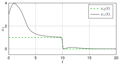
Figure 3: Scenario 1: The black solid line illustrates the actual, the green dashed line the desired value for the state $x_{1}$. The system converges to the desired state over time.

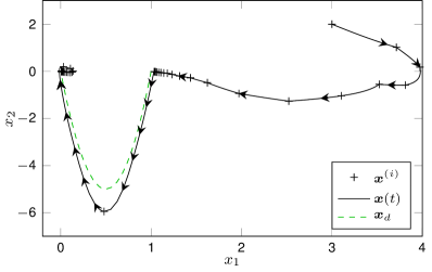
Figure 4: Scenario 1: Black crosses indicate the collected training points, the black solid line illustrates the actual, the green dashed the desired trajectory. The system approaches the desired states as more training points are collected.

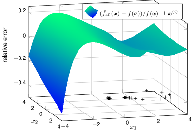
Figure 5: Scenario 1: The surface illustrates the relative error between the true function $f(\boldsymbol{x})$ and the model estimate $\hat{f}_{40}(\boldsymbol{x})$ after taking $40$ training points (black crosses). The error is the lowest (in terms of absolute value) near the training data.

Figure 6: Scenario 1: The surface illustrates the relative error between the true function $g(\boldsymbol{x})$ and the model estimate $\hat{g}_{40}(\boldsymbol{x})$ after taking $40$ training points (black crosses). The error is the lowest (in terms of absolute value) near the training data.

It can be seen, that the two stationary points of the desired trajectory, $(1,0)$ and $(0,0)$, are approached with high precision in the steady state. However, for both it requires a few measurements to be collected in the corresponding area of the state space and the following model updates to achieve this high precision. Once reached the steady state, the time-triggered implementation keeps adding unnecessary data points even though the model already has a high precision in this area. This is improved with the event-triggered model update as illustrated in Scenario 2.

$k_{c}$	$\lambda$	$m_{g}(\boldsymbol{x})$	$\sigma_{\text{on}}^{2}$(S1)	$\sigma_{\text{on}}^{2}$(S2)	$\boldsymbol{x}_{0}$	$\beta$	$r_{\text{min}}$
$1$	$1$	$=2$, $\forall\boldsymbol{x}$	$10^{-6}$	$10^{-16}$	$[3\ 2]^{\intercal}$	7	$10^{-5}$

TABLE I: Simulation parameters

VI-B Scenario 2: Event-triggered updates

In Scenario 2 (S2), the results in Sec. V are illustrated, which utilizes the event-triggered model update described by (53). For this scenario, $g(\boldsymbol{x})$ is assumed to be known (Assumption 5 holds). The reference trajectory

$$x_{d}(t)=\sin(t)$$ (67)

is used, which describes a circle with radius $1$ in the state space. The scenario works on noise free measurements, thus Assumption 7 does hold, however, for numerical stability a minimal noise is assumed ($\sigma_{\text{on}}^{2}=10^{-16}$). The simulation is stopped manually after $T_{\text{sim}}=100$.

As this scenario utilizes Assumption 6, we take the kernel hyperparameters to be known at $\sigma_{f}^{2}=5,l_{1/2,f}^{2}=5$ and do not update these at any of the triggered events. Additionally, we set $\beta_{\kappa}$ constant $\forall_{\kappa}$ and refer to the discussion in Sec. V-D and [28]. Additionally, we enforce a lower bound $r>r_{\text{min}}$ to avoid numerical difficulties.

Figure 8 shows the tracking error until $t=30$, which decreases initially approximately exponentially until a numerical limit is reached. In the event-triggered setup, a total of $51$ events are triggered until sufficient training points are collected around the desired trajectory. This is also visualized in the state space view in Fig. 7. In comparison, the time-triggered approach requires to store $200$ data points and would keep adding points for longer simulations, which the event-based would not.

The time-trigger results in a higher computational burden of the data-driven approach: The event-triggered simulation only takes $\approx 5s$ on a Matlab MATLAB 2019a implementation on a i5-6200U CPU with 2.3GHz and uses $0.20957$MB. The time-triggered approach take $\approx 11s$ and uses $0.47924$MB of memory.

Figure 8 also shows, that the stability criteria in Theorem 3 is fulfilled for the event-triggered case, since $\beta_{\kappa}\sigma_{\kappa}(\boldsymbol{x})\leq k_{c}|r|$ holds for any time. In contrast - for the time-triggered case - this condition is violated frequently, which means that negative definiteness of the common Lyapunov function - and thereby stability - cannot be shown.

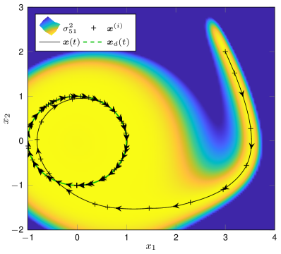
Figure 7: Scenario 2: Black crosses indicate the collected training points, the black solid line illustrates the actual, the green dashed the desired trajectory. The colormap shows the variance function (15) for the GP $\sigma_{51}(\boldsymbol{x})$ after the 51st update, where yellow indicates low variance and blue high variance.

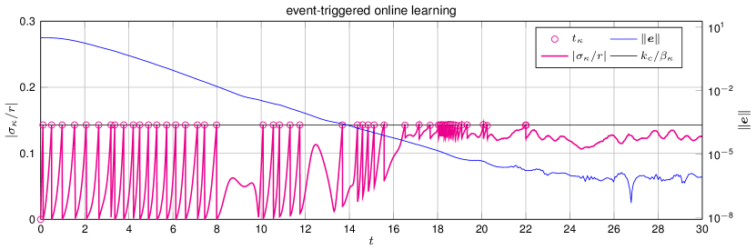
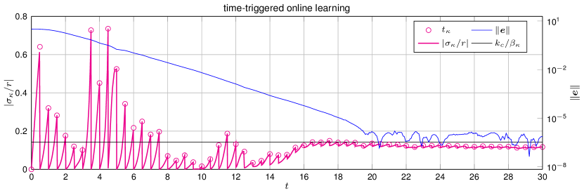
Figure 8: Scenario 2: Comparison of the event-triggered (top) and time-triggered (bottom) online learning. For the first, events (magenta circles) are triggered when the threshold $k_{c}/\beta_{\kappa}$ (black vertical line) is reached by $\sigma_{\kappa}/r$ as proposed in (53). For the latter, events are triggered after a fixed time interval ($\Delta t=0.5$). The blue lines show the norm of the tracking error $\lVert\boldsymbol{e}\rVert$.

VII CONCLUSION

This article proposes an online learning feedback linearizing control law based on Gaussian process models. The closed-loop identification of the initially unknown system exploits the control affine structure by utilizing a composite kernel. The model is updated event-triggered, taking advantage of the uncertainty measure of the GP. The control law results in global asymptotic stability of the tracking error in the noiseless case and in global uniform ultimate boundedness for noisy measurements (of the highest state derivative) with high probability. We therefore propose a safe and data-efficient online learning control approach because model updates occur only if required to ensure stability. Zeno behavior is excluded as a lower bound on the inter-event time is derived. The proposed techniques are illustrated using simulations to support the theoretical results.

Appendix A Expressing structure in kernels

According to [4], the kernel of the GP does not only determine the smoothness properties of the resulting functions but can also be utilized to express prior knowledge regarding the structure of the unknown function.

A-A Sum of functions

Consider $f_{a},f_{b}\colon\mathbb{X}\to\mathbb{R}$ which both originate from two independent GP priors

$$f_{a}(\boldsymbol{x}) \sim\mathcal{GP}\left(m_{a}(\boldsymbol{x}),k_{a}(\boldsymbol{x},\boldsymbol{x}^{\prime})\right),$$ (68)

$$f_{b}(\boldsymbol{x}) \sim\mathcal{GP}\left(m_{b}(\boldsymbol{x}),k_{b}(\boldsymbol{x},\boldsymbol{x}^{\prime})\right),$$ (69)

and add up to $f_{\text{sum}}\colon\mathbb{X}\to\mathbb{R}$, thus $f_{\text{sum}}(\boldsymbol{x})=f_{a}(\boldsymbol{x})+f_{b}(\boldsymbol{x})$. Then,

$$f_{\text{sum}}(\boldsymbol{x})\sim\mathcal{GP}\left(m_{a}(\boldsymbol{x})+m_{b}(\boldsymbol{x}),k_{a}(\boldsymbol{x},\boldsymbol{x}^{\prime})+k_{b}(\boldsymbol{x},\boldsymbol{x}^{\prime})\right)$$ (70)

is also a GP with kernel $k_{a}(\boldsymbol{x},\boldsymbol{x}^{\prime})+k_{b}(\boldsymbol{x},\boldsymbol{x}^{\prime})$.

For regression, where noisy measurements with $\epsilon^{(i)}\sim\mathcal{N}(0,\sigma_{\text{on}}^{2})$ of the sum of the two function are available

$$y_{\text{sum}}^{(i)}=f_{\text{sum}}\left(\boldsymbol{x}^{(i)}\right)+\epsilon^{(i)}=f_{a}\left(\boldsymbol{x}^{(i)}\right)+f_{b}\left(\boldsymbol{x}^{(i)}\right)+\epsilon^{(i)},$$ (71)

with $i=1,\ldots,N$, the joint distribution of the individual functions and the observations is given by

$$\begin{bmatrix}f_{a}(\boldsymbol{x}^{*})\\ f_{b}(\boldsymbol{x}^{*})\\ \boldsymbol{y}_{\text{sum}}\end{bmatrix}\sim\mathcal{N}\left(\boldsymbol{0},\begin{bmatrix}k_{a}^{*}&\boldsymbol{0}&\boldsymbol{k}_{a}^{\intercal}\\ \boldsymbol{0}&k_{b}^{*}&\boldsymbol{k}_{b}^{\intercal}\\ \boldsymbol{k}_{a}&\boldsymbol{k}_{b}&\boldsymbol{K}_{a}+\boldsymbol{K}_{b}+\sigma_{\text{on}}^{2}\boldsymbol{I}_{N}\end{bmatrix}\right),$$ (72)

where the prior mean functions are set to zero $m_{a}(\boldsymbol{x})=m_{b}(\boldsymbol{x})=0$ for notational simplicity and $\boldsymbol{k}_{a},\boldsymbol{k}_{b},k_{a}^{*},k_{b}^{*}$ are defined according to (16). By conditioning, the output of $f_{a}$ and $f_{b}$ are inferred for a test points $\boldsymbol{x}^{*}$

$$\left.f_{a}(\boldsymbol{x}^{*})\right|\boldsymbol{X},\boldsymbol{y}_{\text{sum}} \sim\mathcal{N}\left(\boldsymbol{k}_{a}^{\intercal}\boldsymbol{K}_{\text{sum}}^{-1}\boldsymbol{y}_{\text{sum}},k_{a}^{*}-\boldsymbol{k}_{a}^{\intercal}\boldsymbol{K}_{\text{sum}}^{-1}\boldsymbol{k}_{a}\right),$$ (73)

$$\left.f_{b}(\boldsymbol{x}^{*})\right|\boldsymbol{X},\boldsymbol{y}_{\text{sum}} \sim\mathcal{N}\left(\boldsymbol{k}_{b}^{\intercal}\boldsymbol{K}_{\text{sum}}^{-1}\boldsymbol{y}_{\text{sum}},k_{b}^{*}-\boldsymbol{k}_{b}^{\intercal}\boldsymbol{K}_{\text{sum}}^{-1}\boldsymbol{k}_{b}\right),$$ (74)

where $\boldsymbol{K}_{\text{sum}}=\boldsymbol{K}_{a}+\boldsymbol{K}_{b}+\sigma_{\text{on}}^{2}\boldsymbol{I}_{N}$ with $\boldsymbol{K}_{a},\boldsymbol{K}_{b}$ according to (11). Similarly to (8), the extended hyperparameter vector $\boldsymbol{\psi}_{\text{sum}}=[\boldsymbol{\psi}_{a}^{\intercal}\ \ \boldsymbol{\psi}_{b}^{\intercal}]^{\intercal}$ is obtained through optimization of the likelihood, where $\boldsymbol{K}=\boldsymbol{K}_{\text{sum}}$ and $\boldsymbol{y}_{f}=\boldsymbol{y}_{\text{sum}}$. This allows to predict a value of the individual functions $f_{a},f_{b}$ even though only their sum has been measured.

A-B Product with known function

Consider an unknown function $f_{h}(\boldsymbol{x})\colon\mathbb{X}\to\mathbb{R}$, which is multiplied with the known function $h(\boldsymbol{x})\colon\mathbb{X}\to\mathbb{R}$, we can model $f_{h}$ using a GP with a scaled kernel function and noisy measurements

$$y_{\text{prod}}^{(i)}=f_{\text{prod}}\left(\boldsymbol{x}^{(i)}\right)+\epsilon^{(i)}=f_{h}\left(\boldsymbol{x}^{(i)}\right)h\left(\boldsymbol{x}^{(i)}\right)+\epsilon^{(i)}$$ (75)

of the product with $\epsilon^{(i)}\sim\mathcal{N}(0,\sigma_{\text{on}}^{2}),\ \mbox{$i=1,\ldots,N$ }$. Thus, if $f_{h}\sim\mathcal{GP}(0,k_{h}(\boldsymbol{x},\boldsymbol{x}^{\prime}))$ is a GP, then $f_{\text{prod}}(\boldsymbol{x})$ is also a GP with kernel

$$k_{\text{prod}}(\boldsymbol{x},\boldsymbol{x}^{\prime})=h(\boldsymbol{x})k_{h}(\boldsymbol{x},\boldsymbol{x}^{\prime})h(\boldsymbol{x}^{\prime}),$$ (76)

where the prior mean is set to zero $m_{h}(\boldsymbol{x})=0$ for notational simplicity.

The joint distribution of the measurements and the inferred output of $f_{\text{prod}}$ at a test input $\boldsymbol{x}^{*}$ is given by

$$\begin{bmatrix}f_{h}(\boldsymbol{x}^{*})\\ \boldsymbol{y}_{\text{prod}}\end{bmatrix}\sim\mathcal{N}\left(\boldsymbol{0},\begin{bmatrix}k_{h}^{*}&\boldsymbol{k}_{h}^{\intercal}\boldsymbol{H}^{\intercal}\\ \boldsymbol{H}\boldsymbol{k}_{h}&\boldsymbol{H}^{\intercal}\boldsymbol{K}_{h}\boldsymbol{H}+\sigma_{\text{on}}^{2}\boldsymbol{I}_{N}\end{bmatrix}\right),$$ (77)

where $\boldsymbol{H}=\text{diag}\left(h\left(\boldsymbol{x}^{(1)}\right),\dots,h\left(\boldsymbol{x}^{(N)}\right)\right)\in\mathbb{R}^{N\times N}$ and $\boldsymbol{k}_{h},\ k_{h}^{*}$, $\boldsymbol{K}_{h}$ are defined similarly to (16) and (11), respectively. By conditioning on the training data and the input the function $f_{h}$ is inferred by

$$\left.f_{h}(\boldsymbol{x}^{*})\right|\boldsymbol{X},\boldsymbol{y}_{\text{prod}}\sim\mathcal{N}\big{(}\boldsymbol{k}_{h}^{\intercal}\boldsymbol{H}^{\intercal} \boldsymbol{K}_{\text{prod}}^{\text{-}1}\boldsymbol{y}_{\text{prod}},$$ (78)

$$k_{h}^{*}-\boldsymbol{k}_{h}^{\intercal}\boldsymbol{H}^{\intercal}\boldsymbol{K}_{\text{prod}}^{\text{-}1}\boldsymbol{H}\boldsymbol{k}_{h}\big{)},$$

where $\boldsymbol{K}_{\text{prod}}=\boldsymbol{H}^{\intercal}\boldsymbol{K}_{h}\boldsymbol{H}+\sigma_{\text{on}}^{2}\boldsymbol{I}_{N}$.

Remark 8

Instead of scaling the kernel, it seems more straight forward to use $y_{\text{prod}}^{(i)}/h\left(\boldsymbol{x}^{(i)}\right)$ as training data for a GP with unscaled kernel. However, this would scale the observation noise undesirably, is numerically not stable and is not compatible with the summation of kernels in Appendix A-A, which we combine in our identification approach in Sec. III-B.

Appendix B Improving identification

From Lemma 2 it is known, that the state remains bounded for any finite $0<T<\infty$ without any control input. Thus, without risking damage to the system, one can set $u=0$ for at time interval $T$ and record an open-loop training point

$$y^{(i_{\text{ol}})}=f\left(\boldsymbol{x}^{(i_{\text{ol}})}\right)+\epsilon^{(i_{\text{ol}})},$$ (79)

which is highly beneficial as it only measures $f(\boldsymbol{x})$ (with the usual noise $\epsilon$). The GP framework allows to merge these $i_{\text{ol}}=1,\ldots,N_{\text{ol}}$ observations with the closed-loop training points in $\mathbb{D}_{\kappa}$ to improve the prediction as follows: Consider the extension of the joint distribution (25) (where $u=1$ is assumed in the close loop measurements and $m_{g}(\boldsymbol{x})=0$ for notational convenience)

$$\begin{bmatrix}f(\boldsymbol{x}^{*})\\ g(\boldsymbol{x}^{*})\\ \boldsymbol{y}\\ \boldsymbol{y}_{\text{ol}}\end{bmatrix}\sim\mathcal{N}\left(\boldsymbol{0},\begin{bmatrix}k_{f}^{*}&0&\boldsymbol{k}_{f}^{\intercal}&\boldsymbol{k}_{f,\text{ol}}^{\intercal}\\ 0&k_{g}^{*}&\boldsymbol{k}_{g}^{\intercal}&\boldsymbol{0}_{1\times N_{\text{ol}}}\\ \boldsymbol{k}_{f}&\boldsymbol{k}_{g}&\boldsymbol{K}_{fg}&\boldsymbol{K}_{\text{ol,cl}}^{\intercal}\\ \boldsymbol{k}_{f,\text{ol}}&\boldsymbol{0}_{N_{\text{ol}}\times 1}&\boldsymbol{K}_{\text{ol,cl}}&\boldsymbol{K}_{\text{ol}}\end{bmatrix}\right),$$

where $\boldsymbol{K}_{\text{ol,cl}}$, $\boldsymbol{K}_{\text{ol}}$ are the pairwise evaluation of $k(\boldsymbol{x}^{(i_{\text{ol}})},\boldsymbol{x}^{(i)})$, $k\left(\boldsymbol{x}^{(i_{\text{ol}})},\boldsymbol{x}^{(i^{\prime}_{\text{ol}})}\right)$ and $\boldsymbol{k}_{f,\text{ol}}$ evaluates $k\left(\boldsymbol{x}^{*},\boldsymbol{x}^{(i_{\text{ol}})}\right)$. for all $i=1,\ldots,N$ , $i_{\text{ol}},i^{\prime}_{\text{ol}}=1,\ldots,N_{\text{ol}}$. Then, the estimates are given by

$$\hat{f}(\boldsymbol{x}^{*}) =[\boldsymbol{k}^{\intercal}_{f}\ \boldsymbol{k}^{\intercal}_{f,\text{ol}}]\boldsymbol{\mathcal{K}}^{-1}\tilde{\boldsymbol{y}},\quad\hat{g}(\boldsymbol{x}^{*})=[\boldsymbol{k}^{\intercal}_{g}\ \boldsymbol{0}_{1\times N_{\text{ol}}}]\boldsymbol{\mathcal{K}}^{-1}\tilde{\boldsymbol{y}}$$

$$\text{with }\boldsymbol{\mathcal{K}} =\begin{bmatrix}\boldsymbol{K}_{fg}&\boldsymbol{K}_{\text{ol,cl}}^{\intercal}\\ \boldsymbol{K}_{\text{ol,cl}}&\boldsymbol{K}_{\text{ol}}\end{bmatrix},\text{ and }\tilde{\boldsymbol{y}}=\begin{bmatrix}\boldsymbol{y}\\ \boldsymbol{y}_{\text{ol}}\end{bmatrix}.$$ (80)

We do not further investigate this extension, since it does not provide any additional formal guarantees regarding the convergence, however, in practice, a significant improvement of the identification can be expected.

Jonas Umlauft (S’15) received his B.Sc. and M.Sc. degree in electrical engineering and information technology from the Technical University of Munich, Germany, in 2013 and 2015, respectively. His Master’s thesis was carried out at the Computational and Biological Learning Group at the University of Cambridge, UK. Since May 2015, he is a PhD student at the Chair of Information-oriented Control, Department of Electrical and Computer Engineering at the Technical University of Munich, Germany. His current research interests includes stability of data-driven control systems and system identification based on Gaussian processes.

Sandra Hirche (M’03-SM’11) received the Diplom-Ingenieur degree in aeronautical engineering from Technical University Berlin, Germany, in 2002 and the Doktor-Ingenieur degree in electrical engineering from Technical University Munich, Germany, in 2005. From 2005 to 2007 she was awarded a Postdoc scholarship from the Japanese Society for the Promotion of Science at the Fujita Laboratory, Tokyo Institute of Technology, Tokyo, Japan. From 2008 to 2012 she has been an associate professor at Technical University Munich. Since 2013 she is TUM Liesel Beckmann Distinguished Professor and has the Chair of Information-oriented Control in the Department of Electrical and Computer Engineering at Technical University Munich. Her main research interests include cooperative, distributed and networked control with applications in human-machine interaction, multi-robot systems, and general robotics. She has published more than 150 papers in international journals, books and refereed conferences. Dr. Hirche has served on the Editorial Boards of the IEEE Transactions on Control of Network Systems, IEEE Transactions on Control Systems Technology, and the IEEE Transactions on Haptics. She has received multiple awards such as the Rohde & Schwarz Award for her PhD thesis, the IFAC World Congress Best Poster Award in 2005 and - together with students - the 2018 Outstanding Student Paper Award of the IEEE Conference on Decision and Control as well as Best Paper Awards of IEEE Worldhaptics and IFAC Conference of Manoeuvring and Control of Marine Craft in 2009.

References

- [1] L. Ljung, System Identification. NJ, USA: Prentice Hall PTR, 1998.
- [2] J. Kocijan, Modelling and Control of Dynamic Systems Using Gaussian Process Models. Springer, 2016.
- [3] C. E. Rasmussen and C. K. Williams, Gaussian Processes for Machine Learning. Cambridge, MA, USA: MIT Press, Jan. 2006.
- [4] D. Duvenaud, “Automatic model construction with Gaussian processes,” Ph.D. dissertation, Computational and Biological Learning Laboratory, University of Cambridge, 2014.
- [5] P. A. Ioannou and J. Sun, Robust adaptive control. PTR Prentice-Hall Upper Saddle River, NJ, 1996, vol. 1.
- [6] M. Krstic, I. Kanellakopoulos, P. V. Kokotovic et al., Nonlinear and adaptive control design. Wiley New York, 1995, vol. 222.
- [7] K. J. Åström and B. Wittenmark, Adaptive control. Courier Corporation, 2013.
- [8] A. S. Bazanella, L. Campestrini, and D. Eckhard, Data-driven controller design: the H2 approach. Springer Science & Business Media, 2011.
- [9] G. R. Gonçalves da Silva, A. S. Bazanella, C. Lorenzini, and L. Campestrini, “Data-driven lqr control design,” IEEE Control Systems Letters, vol. 3, no. 1, pp. 180–185, Jan 2019.
- [10] L. Campestrini, D. Eckhard, A. S. Bazanella, and M. Gevers, “Data-driven model reference control design by prediction error identification,” Journal of the Franklin Institute, vol. 354, no. 6, pp. 2628 – 2647, 2017, special issue on recent advances on control and diagnosis via process measurements. [Online]. Available: http://www.sciencedirect.com/science/article/pii/S001600321630271X
- [11] D. A. Bristow, M. Tharayil, and A. G. Alleyne, “A survey of iterative learning control,” IEEE Control Systems Magazine, vol. 26, no. 3, pp. 96–114, Jun. 2006.
- [12] M.-B. Rădac, R.-E. Precup, E. M. Petriu, and S. Preitl, “Iterative data-driven tuning of controllers for nonlinear systems with constraints,” IEEE Transactions on Industrial Electronics, vol. 61, no. 11, pp. 6360–6368, Nov 2014.
- [13] Z. Hou, R. Chi, and H. Gao, “An overview of dynamic-linearization-based data-driven control and applications,” IEEE Transactions on Industrial Electronics, vol. 64, no. 5, pp. 4076–4090, May 2017.
- [14] M. C. Campi and S. M. Savaresi, “Direct nonlinear control design: the virtual reference feedback tuning (vrft) approach,” IEEE Transactions on Automatic Control, vol. 51, no. 1, pp. 14–27, Jan 2006.
- [15] H. Hjalmarsson, M. Gevers, S. Gunnarsson, and O. Lequin, “Iterative feedback tuning: theory and applications,” IEEE Control Systems Magazine, vol. 18, no. 4, pp. 26–41, Aug 1998.
- [16] L. C. Kammer, R. R. Bitmead, and P. L. Bartlett, “Direct iterative tuning via spectral analysis,” Automatica, vol. 36, pp. 1301–1307, 2000.
- [17] N. J. Killingsworth and K. Miroslav, “Pid tuning using extremum seeking: online, model-free performance optimization,” IEEE Control Systems Magazine, vol. 26, no. 1, pp. 70–79, Feb 2006.
- [18] E. Theodorou, J. Buchli, and S. Schaal, “Reinforcement learning of motor skills in high dimensions: A path integral approach,” in International Conference on Robotics and Automation (ICRA). IEEE, May 2010, pp. 2397–2403.
- [19] R. S. Sutton and A. G. Barto, Reinforcement learning: An introduction, 1st ed. Cambridge, MA, USA: MIT Press, 1998.
- [20] M. P. Deisenroth and C. E. Rasmussen, “PILCO: A model-based and data-efficient approach to policy search,” in International Conference on Machine Learning (ICML), 2011, pp. 465–472.
- [21] D. Nguyen-Tuong and J. Peters, “Model learning for robot control: a survey,” Cognitive processing, vol. 12, no. 4, pp. 319–340, 2011.
- [22] D. Nguyen-Tuong, M. Seeger, and J. Peters, “Model learning with local Gaussian process regression,” Advanced Robotics, vol. 23, no. 15, pp. 2015–2034, 2009.
- [23] T. Beckers, J. Umlauft, and S. Hirche, “Stable model-based control with Gaussian process regression for robot manipulators,” in World Congress of the International Federation of Automatic Control (IFAC), vol. 50, no. 1. Elsevier, 2017, pp. 3877–3884.
- [24] Y. Fanger, J. Umlauft, and S. Hirche, “Gaussian processes for dynamic movement primitives with application in knowledge-based cooperation,” in International Conference on Intelligent Robots and Systems (IROS). IEEE, Oct. 2016, pp. 3913–3919.
- [25] T. Beckers, J. Umlauft, D. Kulic, and S. Hirche, “Stable Gaussian process based tracking control of Lagrangian systems,” in Conference on Decision and Control (CDC). IEEE, Dec. 2017, pp. 5180–5185. [Online]. Available: https://ieeexplore.ieee.org/document/8264427
- [26] J. Umlauft, A. Lederer, and S. Hirche, “Learning stable Gaussian process state space models,” in American Control Conference (ACC), IEEE. IEEE, May 2017, pp. 1499–1504. [Online]. Available: https://ieeexplore.ieee.org/document/7963165
- [27] J. Umlauft, L. Pöhler, and S. Hirche, “An uncertainty-based control Lyapunov approach for control-affine systems modeled by Gaussian process,” IEEE Control Systems Letters, vol. 2, no. 3, pp. 483–488, Jul. 2018, outstanding Student Paper Award of the IEEE Conference on Decision and Control. [Online]. Available: https://ieeexplore.ieee.org/document/8368325
- [28] F. Berkenkamp, R. Moriconi, A. Schoellig, and A. Krause, “Safe learning of regions of attraction for uncertain, nonlinear systems with Gaussian processes,” arXiv preprint arXiv:1603.04915, 2016.
- [29] G. Chowdhary, H. A. Kingravi, J. P. How, and P. A. Vela, “Bayesian nonparametric adaptive control using Gaussian processes,” IEEE Transactions on Neural Networks and Learning Systems, vol. 26, no. 3, pp. 537–550, Mar. 2015.
- [30] A. Chakrabortty and M. Arcak, “Robust stabilization and performance recovery of nonlinear systems with unmodeled dynamics,” IEEE Transactions on Automatic Control (TAC), vol. 54, no. 6, pp. 1351–1356, June 2009.
- [31] A. Chakrabortty and M. Arcak, “Time-scale separation redesigns for stabilization and performance recovery of uncertain nonlinear systems,” Automatica, vol. 45, no. 1, pp. 34 – 44, 2009. [Online]. Available: http://www.sciencedirect.com/science/article/pii/S0005109808003701
- [32] M. M. Polycarpou and P. A. Ioannou, Identification and control of nonlinear systems using neural network models: Design and stability analysis. University of Southern Calif., 1991.
- [33] F. L. Lewis, A. Yesildirek, and K. Liu, “Multilayer neural-net robot controller with guaranteed tracking performance,” IEEE Transactions on Neural Networks, vol. 7, no. 2, pp. 388–399, 1996.
- [34] F. L. Lewis, K. Liu, and A. Yesildirek, “Neural net robot controller with guaranteed tracking performance,” IEEE Transactions on Neural Networks, vol. 6, no. 3, pp. 703–715, 1995.
- [35] R. M. Sanner and J.-J. Slotine, “Stable adaptive control and recursive identification using radial Gaussian networks,” in Conference on Decision and Control (CDC). IEEE, 1991, pp. 2116–2123.
- [36] A. Yesildirak and F. L. Lewis, “Feedback linearization using neural networks,” Automatica, vol. 31, no. 11, pp. 1659–1664, 1995.
- [37] J. Umlauft, Y. Fanger, and S. Hirche, “Bayesian uncertainty modeling for programming by demonstration,” in International Conference on Robotics and Automation (ICRA), May 2017, pp. 6428–6434.
- [38] J. Umlauft, T. Beckers, M. Kimmel, and S. Hirche, “Feedback linearization using Gaussian processes,” in Conference on Decision and Control (CDC). IEEE, Dec. 2017, pp. 5249–5255. [Online]. Available: https://ieeexplore.ieee.org/abstract/document/8264435/
- [39] H. K. Khalil and J. Grizzle, Nonlinear systems. Prentice hall New Jersey, 1996, vol. 3.
- [40] M. W. Seeger, S. M. Kakade, and D. P. Foster, “Information consistency of nonparametric Gaussian process methods,” IEEE Transactions on Information Theory, vol. 54, no. 5, pp. 2376–2382, May 2008.
- [41] J. Sherman and W. J. Morrison, “Adjustment of an inverse matrix corresponding to a change in one element of a given matrix,” Ann. Math. Statist., vol. 21, no. 1, pp. 124–127, Mar. 1950. [Online]. Available: https://doi.org/10.1214/aoms/1177729893
- [42] D. Liberzon, Switching in systems and control. Springer Science & Business Media, 2012.
- [43] T. Beckers, D. Kulić, and S. Hirche, “Stable Gaussian process based tracking control of Euler-Lagrange systems,” Automatica, vol. 23, no. 103, pp. 390–397, 2019.
- [44] J.-J. E. Slotine and J. Karl Hedrick, “Robust input-output feedback linearization,” International Journal of Control, vol. 57, no. 5, pp. 1133–1139, 1993.
- [45] N. Srinivas, A. Krause, S. M. Kakade, and M. W. Seeger, “Information-theoretic regret bounds for Gaussian process optimization in the bandit setting,” IEEE Transactions on Information Theory, vol. 58, no. 5, pp. 3250–3265, May 2012.
- [46] D. H. Wolpert, “The supervised learning no-free-lunch theorems,” in Soft Computing and Industry. Springer, 2002, pp. 25–42.
- [47] W. P. M. H. Heemels, K. H. Johansson, and P. Tabuada, “An introduction to event-triggered and self-triggered control,” in Conference on Decision and Control (CDC), Dec. 2012, pp. 3270–3285.
- [48] D. Nguyen-Tuong, J. R. Peters, and M. Seeger, “Local Gaussian process regression for real time online model learning,” in Advances in Neural Information Processing Systems (NIPS), D. Koller, D. Schuurmans, Y. Bengio, and L. Bottou, Eds. Curran Associates, Inc., 2009, pp. 1193–1200.
- [49] J. Umlauft, T. Beckers, and S. Hirche, “A scenario-based optimal control approach for Gaussian process state space models,” in European Control Conference (ECC), 6 2018, pp. 1386–1392. [Online]. Available: https://ieeexplore.ieee.org/document/8550458
- [50] P. Tabuada, “Event-triggered real-time scheduling of stabilizing control tasks,” IEEE Transactions on Automatic Control (TAC), vol. 52, no. 9, pp. 1680–1685, 2007.
- [51] Wolfram—Alpha, “Solution first-order nonlinear ordinary differential equation,” Online, 2018. [Online]. Available: http://www.wolframalpha.com
- [52] P. C. Chu and J. E. Beasley, “A genetic algorithm for the multidimensional knapsack problem,” Journal of heuristics, vol. 4, no. 1, pp. 63–86, 1998.
- [53] F. Lewis, S. Jagannathan, and A. Yesildirak, Neural network control of robot manipulators and non-linear systems. CRC Press, 1998.