Two Efficient Ridge Solutions for the Incremental Broad Learning System on Added Inputs

Abstract

To improve the existing broad learning system (BLS) for new added inputs, this paper proposes the recursive and square-root BLS algorithms that utilize the inverse and inverse Cholesky factor of the Hermitian matrix in the ridge inverse, respectively, to update the ridge solution for the output weights. The recursive BLS updates the inverse by the matrix inversion lemma, while the square-root BLS updates the upper-triangular inverse Cholesky factor by multiplying it with an upper-triangular intermediate matrix. When the added $p$ training samples are more than the total $k$ nodes in the network, i.e., $p>k$, the inverse of a sum of matrices is applied to take a smaller matrix inversion or inverse Cholesky factorization. For the distributed BLS with data-parallelism, we introduce the parallel implementation of the square-root BLS, which is deduced from the parallel implementation of the inverse Cholesky factorization.

The existing BLS based on the generalized inverse with the ridge regression assumes the ridge parameter $\lambda\to 0$ in the ridge inverse. When $\lambda\to 0$ is not satisfied, the numerical experiments show that both the proposed ridge solutions improve the testing accuracy of the existing BLS, and the improvement becomes more significant as $\lambda$ is bigger. For example, the proposed two ridge solutions and the existing BLS achieve the maximum testing accuracies of $90.34\%$ and $90.24\%$ respectively when $\lambda={{10}^{-3}}$ on the NYU object recognition benchmark dataset. On the other hand, compared to the existing BLS, both the proposed BLS algorithms theoretically require less complexities, and are significantly faster in the simulations on the Modified National Institute of Standards and Technology dataset. The speedups in total training time of the recursive and square-root BLS algorithms over the existing BLS are $4.41$ and $6.92$ respectively when $p>k$, and are $2.80$ and $1.59$ respectively when $p<k$.

Compared to the recursive BLS, the square-root BLS requires less complexities when $p>0.82k$, and requires more complexities when $p<0.82k$. If nodes are inserted after each increment of inputs, both the proposed BLS algorithms are applied with the efficient ridge solution based on the inverse Cholesky factor for the BLS on added nodes, to obtain the complete ridge solution. Then the recursive BLS always require more complexities than the square-root BLS, since it requires the extra computations to get the Cholesky factor and multiply the Cholesky factor with its transpose. When $\lambda$ is small in the simulations, the numerical errors caused by those extra computations reduce the testing accuracy or even make the recursive BLS unworkable. On the contrary, the square-root BLS does not need any extra computations and basically achieves the testing accuracy of the direct ridge solution, since it is based on the Cholesky factor just like the efficient ridge solution for the BLS on added nodes.

I Introduction

Single layer feedforward neural networks (SLFN) with the universal approximation capability have been widely applied to solve the classification and regression problems [1, 2, 3]. SLFNs can utilize traditional Gradient-descent-based learning algorithms [4, 5]. However, those Gradient-descent-based algorithms suffer from the time-consuming training process and the local minimum trap, while their generalization performance is sensitive to the training parameters, e.g., learning rate. Then the random vector functional-link neural network (RVFLNN) was proposed [2] to eliminate the drawback of long training process, which trains only the output weights, and generates the input weights and biases randomly. RVFLNN offers the generalization capability in function approximation [3], and has been proven to be a universal approximation for continuous functions on compact sets.

Based on the RVFLNN model, a dynamic step-wise updating algorithm was proposed in [6] to model time-variety data with moderate size. When a new input is encountered or the increment of a new node is required, the dynamic algorithm in [6] only computes the pseudoinverse of that added input or node, to update the output weights easily. The scheme in [6] was improved into Broad Learning System (BLS) in [7], to deal with time-variety big data with high dimension. Then in [8], a mathematical proof of the universal approximation capability of BLS is provided, and several BLS variants were discussed, which include cascade, recurrent, and broad-deep combination structures.

In BLS [7, 8], the previous scheme [6] is improved in three aspects. Firstly, BLS transforms the input data into the feature nodes to reduce the data dimensions. Secondly, BLS can update the output weights easily for any number of new added nodes or inputs, since it only requires one iteration to compute the pseudoinverse of those added nodes or inputs. Lastly, to achieve a better generalization performance, BLS computes the output weights by the generalized inverse with the ridge regression, which assumes the ridge parameter $\lambda\to 0$ in the ridge inverse [9] to approximate the generalized inverse.

To improve the original BLS on added nodes [7], the efficient generalized inverse and ridge solutions [9] were proposed in [10] and [11], respectively, which are both based on the Cholesky factor, while the ridge solution based on the ridge inverse was also proposed in [11]. To improve the original BLS on added inputs [7], an efficient implementation was proposed in [13] to accelerate a step in the generalized inverse of a partitioned matrix. Specifically, the inverse of a sum of matrices [12] was utilized in [13] when the added inputs are more than the total nodes in the network.

In this paper, we propose two efficient BLS algorithms for added inputs, which compute the ridge solution for the output weights. Then the assumption of $\lambda\to 0$ in the original BLS [7] is no longer required, and $\lambda$ can be any positive real number. The proposed BLS algorithms compute the ridge solution from the inverse or inverse Cholesky factor of the Hermitian matrix in the ridge inverse, to avoid spending more complexity to compute the bigger ridge inverse. In the case of more added inputs than the total nodes, the inverse of a sum of matrices [12] is also applied to accelerate several steps in the proposed BLS algorithms, as in [13].

When big data with high dimension is processed, the training processing may exceed the capacity of a single computational node. Accordingly, usually it is required to distribute computing tasks across multiple computational nodes, that are also called as workers [21]. Specifically, a distributed implementation is usually necessary when data is inherently distributed or too big to store on a single worker. It is necessary to choose and implement the algorithms to enable parallel computation in distributed systems. In this paper, we focus on data-parallelism [21], where training samples are partitioned into multiple workers, and nearly the same algorithms are applied to different groups of training samples in all workers. We will develop the parallel implementation of the proposed ridge solution based on inverse Cholesky factor for the distributed BLS with data-parallelism.

This paper is organized as follows. Section ii@ introduces the existing incremental BLS on added inputs based on the generalized inverse with the ridge regression. In Section iii@, we propose two efficient ridge solutions for the BLS on added inputs. Then in Section iv@, we compare the expected computational complexities of the existing BLS and the proposed two ridge solutions, and evaluate them by numerical experiments. Finally, conclusions are given in Section v@.

II Existing Incremental BLS on Added Inputs Based on Generalized Inverse Solution

In RVFLNN, the input data ${{\mathbf{X}}}$ forms the enhancement components by $\xi({{\mathbf{X}}}{{\mathbf{W}}_{{{h}}}}+{{\mathbf{\beta}}_{{{h}}}})$, where ${{\mathbf{W}}_{{{h}}}}$ and ${{\mathbf{\beta}}_{{{h}}}}$ are random, and $\xi$ is the activation function. Then the output

$${\mathbf{\hat{Y}}}={{\mathbf{A}}}{{\mathbf{W}}},$$ (1)

where ${{\mathbf{W}}}$ denotes the output weights, and the expanded input matrix ${{\mathbf{A}}}=\left[{{\mathbf{X}}}|\xi({{\mathbf{X}}}{{\mathbf{W}}_{{{h}}}}+{{\mathbf{\beta}}_{{{h}}}})\right]$. The least-square solution [6] of (1) is the generalized inverse solution [9]

$${{\mathbf{W}}}=\mathbf{A}^{+}\mathbf{Y},$$ (2)

where $\mathbf{Y}$ denotes the labels, and the generalized inverse

$${{\bf{A}}^{+}}={{(\mathbf{A}^{T}\mathbf{A})}^{-1}}\mathbf{A}^{T}.$$ (3)

II-A Ridge Regression Approximation of the Generalized Inverse

The generalized inverse solution (2) is aimed to minimize the training errors. But usually it can not achieve the minimum generalization errors, especially for ill-conditioned problems. To achieve a better generalization performance, instead of the generalized inverse solution (2), an alternative solution can be utilized, i.e., the ridge solution [9]

$${\mathbf{\tilde{W}}}={{\bf{A}}^{\dagger}}{{\mathbf{Y}}},$$ (4)

where the ridge inverse [9]

$${{\bf{A}}^{\dagger}}={{\left({{\bf{A}}^{T}}{\bf{A}}+\lambda\mathbf{I}\right)}^{-1}}{{\bf{A}}^{T}}.$$ (5)

The ridge inverse (5) degenerates [7, Eq. (3)] into the generalized inverse when the ridge parameter $\lambda\to 0$, i.e.,

$$\underset{\lambda\to 0}{\mathop{\lim}}\,\mathbf{A}^{\dagger}=\underset{\lambda\to 0}{\mathop{\lim}}\,{{(\mathbf{A}^{T}\mathbf{A}+\lambda\mathbf{I})}^{-1}}\mathbf{A}^{T}=\mathbf{A}^{+},$$ (6)

which is the ridge regression approximation of the generalized inverse. In [7], $\mathbf{A}^{+}$ in the output weights (2) is computed from (6) instead of (3), to improve the generalization performance.

II-B Broad Learning Model

The BLS transfers the original input data $\mathbf{X}$ into the mapped features in the feature nodes, and then enhances the feature nodes as the enhancement nodes. The connections of all the feature and enhancement nodes are fed into the output finally.

In the BLS, the input data $\mathbf{X}$ is projected by

$${{\mathbf{Z}}_{i}}=\phi(\mathbf{X}{{\mathbf{W}}_{{{e}_{i}}}}+{{\mathbf{\beta}}_{{{e}_{i}}}}),$$ (7)

to become the $i$-th group of mapped features ${{\mathbf{Z}}_{i}}$, where the weights ${{\mathbf{W}}_{{{e}_{i}}}}$ and the biases ${{\mathbf{\beta}}_{{{e}_{i}}}}$ are randomly generated and then fine-tuned by applying the linear inverse problem [7]. All the $n$ groups of mapped features are concatenated into

$${{\mathbf{Z}}^{n}}\equiv\left[\begin{matrix}{{\mathbf{Z}}_{1}}&\cdots&{{\mathbf{Z}}_{n}}\\ \end{matrix}\right].$$ (8)

Then all the mapped features ${{\mathbf{Z}}^{n}}$ are enhanced to become the $j$-th group of enhancement nodes ${{\mathbf{H}}_{j}}$, by

$${{\mathbf{H}}_{j}}=\xi({{\mathbf{Z}}^{n}}{{\mathbf{W}}_{{{h}_{j}}}}+{{\mathbf{\beta}}_{{{h}_{j}}}})$$ (9)

where ${{\mathbf{W}}_{{{h}_{j}}}}$ and ${{\mathbf{\beta}}_{{{h}_{j}}}}$ are random. All the $m$ groups of enhancement nodes are concatenated into

$${{\mathbf{H}}^{m}}\equiv\left[{{\mathbf{H}}_{1}},\cdots,{{\mathbf{H}}_{m}}\right].$$ (10)

Finally, all the feature and enhancement nodes are fed into the output by

$$\mathbf{\hat{Y}}=\left[{{\mathbf{Z}}^{n}}|{{\mathbf{H}}^{m}}\right]{{\mathbf{W}}_{n}^{m}}={\bf{A}}_{n}^{m}{{\mathbf{W}}_{n}^{m}},$$ (11)

where the expanded input matrix

$${\bf{A}}_{n}^{m}=\left[{{\mathbf{Z}}^{n}}|{{\mathbf{H}}^{m}}\right],$$ (12)

and the desired connection weights ${{\mathbf{W}}_{n}^{m}}$ are computed by (2) from $({\bf{A}}_{n}^{m})^{+}$, the generalized inverse with the ridge regression.

II-C Incremental Learning for Added Inputs

The BLS includes the incremental learning for the additional input training samples. When encountering new input samples with the corresponding output labels, the modeled BLS can be remodeled in an incremental way without a complete retraining process. It updates the output weights incrementally, without retraining the whole network from the beginning.

Assume that the expanded input matrix ${\bf{A}}_{n}^{m}$ is $l\times k$, where $l$ is the number of training samples, and $k$ is the total number of feature and enhancement nodes. Then we can write ${\bf{A}}_{n}^{m}$ and the corresponding input data ${{\mathbf{X}}}$ as $\mathbf{A}_{{\bar{l}}}$ and $\mathbf{X}_{{\bar{l}}}$, respectively. Similarly, the additional input data can be denoted as ${{\mathbf{X}}_{\bar{p}}}$ with $p$ samples . In BLS, ${{\mathbf{X}}_{\bar{p}}}$ is projected by (7) to get the additional samples for the $i$-th group of feature nodes, which are concatenated into

$$\mathbf{Z}_{\bar{p}}^{n}=\left[\phi({{\mathbf{X}}_{\bar{p}}}{{\mathbf{W}}_{{{e}_{1}}}}+{{\mathbf{\beta}}_{{{e}_{1}}}}),\cdots,\phi({{\mathbf{X}}_{\bar{p}}}{{\mathbf{W}}_{{{e}_{n}}}}+{{\mathbf{\beta}}_{{{e}_{n}}}})\right]$$ (13)

by (8). $\mathbf{Z}_{\bar{p}}^{n}$ is enhanced by (9) and then concatenated by (10). Accordingly, the additional samples for the expanded input matrix can be written as ${\bf{A}}_{\bar{p}}\in{\Re^{p\times k}}$ satisfying

$$\mathbf{A}_{\bar{p}}=\\ \left[\mathbf{Z}_{\bar{p}}^{n}|\xi(\mathbf{Z}_{\bar{p}}^{n}{{\mathbf{W}}_{{{h}_{1}}}}+{{\mathbf{\beta}}_{{{h}_{1}}}}),\cdots,\xi(\mathbf{Z}_{\bar{p}}^{n}{{\mathbf{W}}_{{{h}_{m}}}}+{{\mathbf{\beta}}_{{{h}_{m}}}})\right],$$ (14)

which is utilized to update $\mathbf{A}_{{\bar{l}}}$ into

$${\bf{A}}_{\bar{l}+\bar{p}}={\left[{\begin{array}[]{*{20}{c}}{{\bf{A}}_{\bar{l}}^{T}}&{{\bf{\bar{A}}}_{\bar{p}}^{T}}\end{array}}\right]^{T}}.$$ (15)

In the stepwise updating algorithm in [7], the generalized inverse of $\mathbf{A}_{{\bar{l}}}$ is updated into that of ${\bf{A}}_{\bar{l}+\bar{p}}$ by

$${{\bf{A}}_{\bar{l}+\bar{p}}^{+}}=\left[\begin{matrix}{{\bf{A}}_{\bar{l}}^{+}}-{{\mathbf{B}}}{{\mathbf{D}}^{T}}&{{\mathbf{B}}}\\ \end{matrix}\right],$$ (16)

where

$${{\mathbf{D}}^{T}}=\mathbf{A}_{\bar{p}}{{\bf{A}}_{\bar{l}}^{+}},$$ (17)

$$\mathbf{{C}}=\mathbf{A}_{\bar{p}}^{{T}}-{\bf{A}}_{\bar{l}}^{T}{{\mathbf{D}}},$$ (18)

and

$${{\bf{B}}}= ({{\bf{C}}^{+}})^{T}\ \quad\quad\quad\quad\quad\quad if\ {{\bf{C}}\neq{\bf{0}}}$$ (19a)

$${{\bf{B}}}= {{{\bf{A}}_{\bar{l}}^{+}}{{\bf{D}}}{{({\bf{I}}+{{\bf{D}}^{T}}{\bf{D}})}^{-1}}\quad if\ {\bf{C}}={\bf{0}}}.$$ (19b)

Then the output weights $\mathbf{W}_{\bar{l}}$ is updated into ${\mathbf{W}}_{\bar{l}+\bar{p}}$ by

$${\mathbf{W}}_{\bar{l}+\bar{p}}=\mathbf{W}_{\bar{l}}+{{\mathbf{B}}}({{\mathbf{Y}}_{\bar{p}}}-\mathbf{A}_{\bar{p}}\mathbf{W}_{\bar{l}}),$$ (20)

which is the generalized inverse solution.

Since it is impossible to observe any input matrix that is rank deficient in practice [6, pp. 64], we assume the expanded input matrix $\mathbf{A}_{{\bar{l}}}$ is of full rank in this paper. Moreover, we focus on the usual case where the $l\times k$ matrix $\mathbf{A}_{{\bar{l}}}$ satisfies

$$l>k,$$ (21)

i.e., the training samples are more than the total nodes, as in  [7, 13]. Then ${\bf{C}}={\bf{0}}$ can be concluded [6, pp. 64] for ${\bf{C}}$ computed by (18) from $\mathbf{A}_{{\bar{l}}}\in{\Re^{l\times k}}$ with $l>k$.

For the usual case with ${\bf{C}}={\bf{0}}$, the complexity of the BLS on added inputs was reduced in [13] by modifying (19) into

$${{\bf{B}}}= {{{\bf{C}}^{+}}\quad\quad\quad\quad\quad\quad\quad\quad\ \,if\ {\bf{C}}\neq{\bf{0}}}$$ (22a)

$${{\bf{B}}}= {\bf{\bar{D}}}{{({\bf{I}}+{\bf{A}}_{\bar{p}}{\bf{\bar{D}}})}^{-1}}\quad\quad\quad\ if\ {\bf{C}}={\bf{0}}\And p\leq k$$ (22b)

$${{\bf{B}}}= {{({\bf{I}}+{\bf{\bar{D}}}{\bf{A}}_{\bar{p}})}^{-1}}{\bf{\bar{D}}}\quad\quad\quad\ if\ {\bf{C}}={\bf{0}}\And p\geq k,$$ (22c)

where $p$ and $k$ are the size of ${\bf{A}}_{\bar{p}}\in{\Re^{p\times k}}$, and

$${\bf{\bar{D}}}={{\bf{A}}_{\bar{l}}^{+}}{{\bf{D}}}.$$ (23)

Obviously, (22b) for the case of $p\leq k$ contains only minor changes to (19b). Moreover, the inverse of a sum of matrices [12] is utilized to deduce (22c) for the case of $p\geq k$ with the $k\times k$ matrix inverse, which is usually more efficient than (19b) with the $p\times p$ matrix inverse.

II-D Construction Model and Learning Procedure of BLS

In Algorithms 1 and 2, we summarize the construction model and learning procedure of the existing BLS algorithm on added inputs, which includes the improvement proposed in [13]. Algorithm 1 lists the construction model and the procedure to compute the initial expanded input matrix $\mathbf{A}_{{\bar{l}}}$, while Algorithm 2 lists the procedure to compute the output weights and the incremental learning for added inputs.

Algorithm 1 : The Broad Learning Algorithm: Computation of the Initial Expanded Input Matrix

1:Training samples $\mathbf{X}_{{\bar{l}}}$

2:Expanded input matrix $\mathbf{A}_{{\bar{l}}}={\bf{A}}_{n}^{m}$

3:for $i=1:n$ do

4:     Fine-tune random ${{\mathbf{W}}_{{{e}_{i}}}}$ and ${{\bm{\beta}}_{{{e}_{i}}}}$;

5:     Compute ${{\mathbf{Z}}_{i}}=\phi(\mathbf{X}_{{\bar{l}}}{{\mathbf{W}}_{{{e}_{i}}}}+{{\bm{\beta}}_{{{e}_{i}}}})$;

6:end for

7:Concatenate the feature nodes into ${{\mathbf{Z}}^{n}}\equiv\left[\begin{matrix}{{\mathbf{Z}}_{1}}&\cdots&{{\mathbf{Z}}_{n}}\\ \end{matrix}\right]$;

8:for $j=1:m$ do

9:     Random ${{\mathbf{W}}_{{{h}_{j}}}}$ and ${{\bm{\beta}}_{{{h}_{j}}}}$;

10:     Compute ${{\mathbf{H}}_{j}}=\xi({{\mathbf{Z}}^{n}}{{\mathbf{W}}_{{{h}_{j}}}}+{{\bm{\beta}}_{{{h}_{j}}}})$;

11:end for

12:Set the enhancement nodes group ${{\mathbf{H}}^{m}}\equiv\left[{{\mathbf{H}}_{1}},\cdots,{{\mathbf{H}}_{m}}\right]$;

13:Set ${{\mathbf{A}}_{n}^{m}}=\left[{{\mathbf{Z}}^{n}}|{{\mathbf{H}}^{m}}\right]$, and write ${{\mathbf{A}}_{n}^{m}}$ as $\mathbf{A}_{{\bar{l}}}$;

Algorithm 2 : The Existing Broad Learning Algorithm: Computation of Output Weights and Increment of Inputs

1:Expanded input matrix $\mathbf{A}_{{\bar{l}}}$, labels $\mathbf{Y}_{{\bar{l}}}$, added inputs ${{\mathbf{X}}_{\bar{p}}}$ and labels ${{\mathbf{Y}}_{\bar{p}}}$

2:Output weights $\mathbf{W}$

3:Compute $\mathbf{A}_{{\bar{l}}}^{+}$ and $\mathbf{W}_{{\bar{l}}}$ by (6) and (2), respectively;

4:while The target training error is not reached do

5:     Use added inputs ${{\mathbf{X}}_{\bar{p}}}$ to get $\mathbf{A}_{\bar{p}}$ by (13) and (14);

6:     Update ${{\bf{A}}_{\bar{l}}^{+}}$ into ${{\bf{A}}_{\bar{l}+\bar{p}}^{+}}$ by (16)-(18), (22) and (23);

7:     Update $\mathbf{W}_{{\bar{l}}}$ into $\mathbf{W}_{{\bar{l}}+{\bar{p}}}$ by (20);

8:     $l\Leftarrow l+p$;

9:end while

10:Set $\mathbf{W}=\mathbf{W}_{{\bar{l}}}$;

TABLE I: Comparison of Flops among the BLS Algorithms

		Existing BLS		Proposed Recursive BLS		Proposed Square-Root BLS
Initialization		(6)	$3k^{2}l+k^{3}$	(24)	$k^{2}l+k^{3}$	(38)	$k^{2}l+\frac{2}{3}k^{3}$
3-8		(2)	$2klc$	(26)	$2klc+2k^{2}c$	(39)	$2klc+2k^{2}c$
		Total	$3k^{2}l+k^{3}$ $+2klc\approx$	Total	$k^{2}l+k^{3}+$ $2klc+2k^{2}c\approx$	Total	$k^{2}l+\frac{2}{3}k^{3}+$ $2klc+2k^{2}c\approx$
4-4 6-6 8-8			$3k^{2}l+k^{3}$		$k^{2}l+k^{3}$		$k^{2}l+\frac{2}{3}k^{3}$
Each Update for Incremental Learning		(20)	$4cpk$	${{\mathbf{Q}}_{\bar{l}}}\mathbf{A}_{\bar{p}}^{T}=$ $(\mathbf{A}_{\bar{p}}{{\mathbf{Q}}_{\bar{l}}})^{T}$	$2k^{2}p$	(41)	$pk^{2}$
3-4 7-8		(17), (18),(23), (16)	$2pkl\times 4$			(44)	$k^{3}/3$
	$p<k$	(22b)	$4p^{2}k+p^{3}$	(30)	$3kp^{2}+p^{3}$	${{\mathbf{S}}}{{(\mathbf{I}+{{\mathbf{S}}^{T}}\mathbf{S})}^{-1}}$	$pk^{2}+p^{3}+2p^{2}k$
5-8				(29)	$k^{2}p$	(50a)	$pk^{2}+k^{3}/3$
5-8				(32)	$4cpk$	(50b)	$4cpk+ck^{2}$
		Total	$8pkl+4p^{2}k$ $+p^{3}+4cpk\approx$	Total	$3pk^{2}+3p^{2}k$ $+p^{3}+4cpk\approx$	Total	$\frac{2}{3}k^{3}+3pk^{2}+2p^{2}k$ $+p^{3}+ck^{2}+4cpk\approx$
4-4 6-6 8-8			$8pkl+4p^{2}k+p^{3}$		$3pk^{2}+3p^{2}k+p^{3}$		$\frac{2}{3}k^{3}+3pk^{2}+2p^{2}k+p^{3}$
	$p\geq k$	(22c)	$4k^{2}p+k^{3}$	(35)	$2kp^{2}+3k^{3}$	(67)	$pk^{2}+\frac{2}{3}k^{3}$
5-8				(37)	$4cpk+2ck^{2}$	(70)	$4cpk+2ck^{2}$
		Total	$8pkl+4k^{2}p$ $+k^{3}+4cpk\approx$	Total	$2kp^{2}+2k^{2}p+$ $3k^{3}+2ck^{2}+4cpk\approx$	Total	$2k^{2}p+k^{3}+$ $2ck^{2}+4cpk\approx$
4-4 6-6 8-8			$8pkl+4k^{2}p+k^{3}$		$2kp^{2}+2k^{2}p+3k^{3}$		$2k^{2}p+k^{3}$

III Proposed Two Ridge Solutions for Incremental BLS on Added Inputs

The BLS in [7] utilizes the ridge regression to approximate the generalized inverse $\mathbf{A}^{+}$, and then $\lambda$ must be very small (e.g., $\lambda={{10}^{-8}}$) in (6) to satisfy the assumption of $\lambda\to 0$. In this paper, we develop the algorithms based on the ridge inverse (5) and the ridge solution (4). Accordingly, the assumption of $\lambda\to 0$ for the original BLS [7] is no longer required, and $\lambda$ can be set to any positive real number.

For the BLS in the usual case of $l>k$, we propose a recursive algorithm and a square-root algorithm, which are based on the $k\times k$ Hermitian matrix ${{\bf{A}}^{T}}{\bf{A}}+\lambda\mathbf{I}$ in the ridge inverse (5), and iteratively update its inverse and inverse Cholesky factor , respectively. To reduce the complexity, both the proposed algorithms avoid computing the $k\times(l+p)$ ridge inverse ${\bf{A}}_{\bar{l}+\bar{p}}^{\dagger}$, which is bigger than the $k\times k$ Hermitian matrix.

The proposed recursive BLS algorithm updates the inverse recursively by the matrix inversion lemma [14], while the proposed square-root BLS algorithm updates the inverse Cholesky factor by multiplying it with an upper-triangular intermediate matrix. When there are more rows than columns in the newly added input matrix ${\bf{A}}_{\bar{p}}\in{\Re^{p\times k}}$, i.e., $p>k$, the inverse of a sum of matrices [12] is utilized in the proposed algorithms to compute the intermediate variables by a smaller matrix inversion or inverse Cholesky factorization.

III-A Proposed Recursive BLS Algorithm Based on Inverse of the Hermitian Matrix in the Ridge Inverse

Let us define the $k\times k$ inverse matrix

$${{\mathbf{Q}}_{\bar{l}}}={{\left({{\bf{A}}_{\bar{l}}^{T}}{\bf{A}}_{\bar{l}}+\lambda\mathbf{I}\right)}^{-1}}$$ (24)

to write (5) as

$${{\bf{A}}_{\bar{l}}^{\dagger}}={{\mathbf{Q}}_{\bar{l}}}{{\bf{A}}_{\bar{l}}^{T}},$$ (25)

which can be substituted into (4) to obtain

$${\mathbf{\tilde{W}}}_{\bar{l}}={{\mathbf{Q}}_{\bar{l}}}{{\bf{A}}_{\bar{l}}^{T}}{{\mathbf{Y}}_{\bar{l}}}.$$ (26)

To compute ${{\mathbf{Q}}_{\bar{l}+\bar{p}}}$ from ${{\mathbf{Q}}_{\bar{l}}}$, substitute (15) into (24) to obtain

$${{\mathbf{Q}}_{\bar{l}+\bar{p}}}={{\left(\left({{\bf{A}}_{\bar{l}}^{T}}{\bf{A}}_{\bar{l}}+\lambda\mathbf{I}\right)-\mathbf{A}_{\bar{p}}^{T}(-\mathbf{A}_{\bar{p}})\right)}^{-1}},$$ (27)

into which apply the matrix inversion lemma [14, Eq. (1a)]

$${({\bf{A}}-{\bf{UBV}})^{-1}}={{\bf{A}}^{-1}}+{{\bf{A}}^{-1}}{\bf{U}}{({{\bf{B}}^{-1}}-{\bf{V}}{{\bf{A}}^{-1}}{\bf{U}})^{-1}}{\bf{V}}{{\bf{A}}^{-1}},$$

to obtain

$${{\mathbf{Q}}_{\bar{l}+\bar{p}}} ={{\mathbf{Q}}_{\bar{l}}}+{{\mathbf{Q}}_{\bar{l}}}\mathbf{A}_{\bar{p}}^{T}{{(\mathbf{I}-(-\mathbf{A}_{\bar{p}}){{\mathbf{Q}}_{\bar{l}}}\mathbf{A}_{\bar{p}}^{T})}^{-1}}(-\mathbf{A}_{\bar{p}}){{\mathbf{Q}}_{\bar{l}}}$$

$$={{\mathbf{Q}}_{\bar{l}}}-{{\mathbf{Q}}_{\bar{l}}}\mathbf{A}_{\bar{p}}^{T}{{(\mathbf{I}+\mathbf{A}_{\bar{p}}{{\mathbf{Q}}_{\bar{l}}}\mathbf{A}_{\bar{p}}^{T})}^{-1}}\mathbf{A}_{\bar{p}}{{\mathbf{Q}}_{\bar{l}}}.$$ (28)

Then we simplify (28) into

$${{\mathbf{Q}}_{\bar{l}+\bar{p}}}={{\mathbf{Q}}_{\bar{l}}}-{{\mathbf{\tilde{B}}}}\mathbf{A}_{\bar{p}}{{\mathbf{Q}}_{\bar{l}}},$$ (29)

where the intermediate result ${{\mathbf{\tilde{B}}}}$ is defined by

$${{\mathbf{\tilde{B}}}}={{\mathbf{Q}}_{\bar{l}}}\mathbf{A}_{\bar{p}}^{T}{{(\mathbf{I}+\mathbf{A}_{\bar{p}}{{\mathbf{Q}}_{\bar{l}}}\mathbf{A}_{\bar{p}}^{T})}^{-1}}.$$ (30)

The above ${{\mathbf{\tilde{B}}}}$ can be applied to update ${{\bf{A}}_{\bar{l}}^{\dagger}}$ into ${{\bf{A}}_{\bar{l}+\bar{p}}^{\dagger}}$ by

$${{\bf{A}}_{\bar{l}+\bar{p}}^{\dagger}}=\left[\begin{matrix}{{\bf{A}}_{\bar{l}}^{\dagger}}-{{\mathbf{\tilde{B}}}}\mathbf{A}_{\bar{p}}{{\bf{A}}_{\bar{l}}^{\dagger}}&{{\mathbf{\tilde{B}}}}\\ \end{matrix}\right],$$ (31)

which is deduced in Appendix A. Then (31) and ${{\mathbf{Y}}_{\bar{l}+\bar{p}}}={\left[{\begin{array}[]{*{20}{c}}{{\bf{Y}}_{\bar{l}}^{T}}&{{\bf{Y}}_{\bar{p}}^{T}}\end{array}}\right]^{T}}$ are substituted into (4) to obtain ${\mathbf{\tilde{W}}}_{\bar{l}+\bar{p}}=\left[\begin{matrix}{{\bf{A}}_{\bar{l}}^{\dagger}}-{{\mathbf{\tilde{B}}}}\mathbf{A}_{\bar{p}}{{\bf{A}}_{\bar{l}}^{\dagger}}&{{\mathbf{\tilde{B}}}}\\ \end{matrix}\right]{\left[{\begin{array}[]{*{20}{c}}{{\bf{Y}}_{\bar{l}}^{T}}&{{\bf{Y}}_{\bar{p}}^{T}}\end{array}}\right]^{T}}={{\bf{A}}_{\bar{l}}^{\dagger}}\mathbf{Y}_{{\bar{l}}}-{{\mathbf{\tilde{B}}}}\mathbf{A}_{\bar{p}}{{\bf{A}}_{\bar{l}}^{\dagger}}\mathbf{Y}_{{\bar{l}}}+{{\mathbf{\tilde{B}}}}{{\mathbf{Y}}_{\bar{p}}}$, into which substitute (4) to deduce

$${\mathbf{\tilde{W}}}_{\bar{l}+\bar{p}} =\mathbf{\tilde{W}}_{\bar{l}}-{{\mathbf{\tilde{B}}}}\mathbf{A}_{\bar{p}}\mathbf{\tilde{W}}_{\bar{l}}+{{\mathbf{\tilde{B}}}}{{\mathbf{Y}}_{\bar{p}}}$$

$$=\mathbf{\tilde{W}}_{\bar{l}}+{{\mathbf{\tilde{B}}}}\left({{\mathbf{Y}}_{\bar{p}}}-\mathbf{A}_{\bar{p}}\mathbf{\tilde{W}}_{\bar{l}}\right).$$ (32)

TABLE II: Testing Accuracy of the BLS Algorithms on MNIST Dataset with $p=10000>k=5100$

Number of Inputs			10000	$\xrightarrow[\scriptscriptstyle{10000}]{}$ 20000	$\xrightarrow[\scriptscriptstyle{10000}]{}$ 30000	$\xrightarrow[\scriptscriptstyle{10000}]{}$ 40000	$\xrightarrow[\scriptscriptstyle{10000}]{}$ 50000	$\xrightarrow[\scriptscriptstyle{10000}]{}$ 60000
Testing Accuracy ($\%$)	$\lambda=$ ${{10}^{-8}}$	Exst.	97.57 ($\pm$ 0.114 )	98.27 ($\pm$ 0.069 )	98.45 ($\pm$ 0.061 )	98.56 ($\pm$ 0.064 )	98.59 ($\pm$ 0.058 )	98.64 ($\pm$ 0.058 )
		Recur.	97.57 ($\pm$ 0.114 )	98.27 ($\pm$ 0.072 )	98.45 ($\pm$ 0.060 )	98.56 ($\pm$ 0.063 )	98.58 ($\pm$ 0.060 )	98.64 ($\pm$ 0.056 )
3-9		Sqrt.	97.57 ($\pm$ 0.114 )	98.27 ($\pm$ 0.069 )	98.45 ($\pm$ 0.061 )	98.56 ($\pm$ 0.064 )	98.59 ($\pm$ 0.061 )	98.64 ($\pm$ 0.058 )
3-9		D-Rdg	97.57 ($\pm$ 0.114 )	98.27 ($\pm$ 0.069 )	98.45 ($\pm$ 0.061 )	98.56 ($\pm$ 0.064 )	98.59 ($\pm$ 0.061 )	98.64 ($\pm$ 0.058 )
	$\lambda=$ ${{10}^{-7}}$	Exst.	97.76 ($\pm$ 0.085 )	98.27 ($\pm$ 0.070 )	98.43 ($\pm$ 0.065 )	98.53 ($\pm$ 0.070 )	98.55 ($\pm$ 0.059 )	98.61 ($\pm$ 0.053 )
		Recur.	97.76 ($\pm$ 0.085 )	98.28 ($\pm$ 0.066 )	98.44 ($\pm$ 0.057 )	98.55 ($\pm$ 0.063 )	98.57 ($\pm$ 0.055 )	98.63 ($\pm$ 0.054 )
3-9		Sqrt., D-Rdg	97.76 ($\pm$ 0.085 )	98.28 ($\pm$ 0.067 )	98.44 ($\pm$ 0.057 )	98.55 ($\pm$ 0.064 )	98.57 ($\pm$ 0.055 )	98.63 ($\pm$ 0.055 )
	$\lambda=$ ${{10}^{-6}}$	Exst.	97.76 ($\pm$ 0.081 )	98.13 ($\pm$ 0.094 )	98.28 ($\pm$ 0.092 )	98.39 ($\pm$ 0.072 )	98.41 ($\pm$ 0.083 )	98.46 ($\pm$ 0.079 )
		Recur.	97.76 ($\pm$ 0.081 )	98.19 ($\pm$ 0.078 )	98.36 ($\pm$ 0.079 )	98.47 ($\pm$ 0.066 )	98.51 ($\pm$ 0.059 )	98.56 ($\pm$ 0.059 )
3-9		Sqrt., D-Rdg	97.76 ($\pm$ 0.081 )	98.19 ($\pm$ 0.077 )	98.36 ($\pm$ 0.079 )	98.47 ($\pm$ 0.066 )	98.51 ($\pm$ 0.059 )	98.56 ($\pm$ 0.058 )
	$\lambda=$ ${{10}^{-5}}$	Exst.	97.49 ($\pm$ 0.105 )	97.82 ($\pm$ 0.120 )	97.96 ($\pm$ 0.122 )	98.07 ($\pm$ 0.113 )	98.09 ($\pm$ 0.125 )	98.13 ($\pm$ 0.113 )
		Recur., Sqrt., D-Rdg	97.49 ($\pm$ 0.105 )	97.93 ($\pm$ 0.103 )	98.11 ($\pm$ 0.104 )	98.24 ($\pm$ 0.090 )	98.27 ($\pm$ 0.093 )	98.33 ($\pm$ 0.097 )
	$\lambda=$ ${{10}^{-4}}$	Exst.	96.96 ($\pm$ 0.172 )	97.21 ($\pm$ 0.190 )	97.35 ($\pm$ 0.190 )	97.45 ($\pm$ 0.187 )	97.46 ($\pm$ 0.170 )	97.52 ($\pm$ 0.170 )
		Recur., Sqrt., D-Rdg	96.96 ($\pm$ 0.172 )	97.38 ($\pm$ 0.180 )	97.60 ($\pm$ 0.161 )	97.74 ($\pm$ 0.165 )	97.77 ($\pm$ 0.155 )	97.85 ($\pm$ 0.143 )
	$\lambda=$ ${{10}^{-3}}$	Exst.	96.03 ($\pm$ 0.260 )	96.24 ($\pm$ 0.259 )	96.37 ($\pm$ 0.260 )	96.48 ($\pm$ 0.251 )	96.50 ($\pm$ 0.251 )	96.58 ($\pm$ 0.253 )
		Recur., Sqrt., D-Rdg	96.03 ($\pm$ 0.260 )	96.46 ($\pm$ 0.238 )	96.69 ($\pm$ 0.231 )	96.87 ($\pm$ 0.228 )	96.96 ($\pm$ 0.218 )	97.08 ($\pm$ 0.214 )
	$\lambda=$ ${{10}^{-2}}$	Exst.	94.55 ($\pm$ 0.423 )	94.81 ($\pm$ 0.380 )	94.94 ($\pm$ 0.373 )	95.05 ($\pm$ 0.369 )	95.12 ($\pm$ 0.346 )	95.20 ($\pm$ 0.347 )
		Recur., Sqrt., D-Rdg	94.55 ($\pm$ 0.423 )	95.15 ($\pm$ 0.344 )	95.44 ($\pm$ 0.312 )	95.65 ($\pm$ 0.306 )	95.77 ($\pm$ 0.290 )	95.92 ($\pm$ 0.281 )
	$\lambda=$ ${{10}^{-1}}$	Exst.	92.31 ($\pm$ 0.535 )	92.65 ($\pm$ 0.506 )	92.80 ($\pm$ 0.486 )	92.94 ($\pm$ 0.491 )	93.05 ($\pm$ 0.483 )	93.13 ($\pm$ 0.482 )
		Recur., Sqrt., D-Rdg	92.31 ($\pm$ 0.535 )	93.15 ($\pm$ 0.468 )	93.52 ($\pm$ 0.463 )	93.83 ($\pm$ 0.450 )	94.07 ($\pm$ 0.433 )	94.23 ($\pm$ 0.417 )

When the added training samples are more than the total nodes, i.e., $p>k$, the $p\times p$ matrix inverse in (30) for computing ${{\mathbf{\tilde{B}}}}$ can be simplified into a smaller $k\times k$ inverse, by applying the inverse of a sum of matrices [12, Eq. (20)]

$${{(\mathbf{I}+\mathbf{P}{{\mathbf{Q}}})}^{-1}}\mathbf{P}=\mathbf{P}{{(\mathbf{I}+{{\mathbf{Q}}}\mathbf{P})}^{-1}}$$ (33)

to write (30) as

$${{\mathbf{\tilde{B}}}}={{(\mathbf{I}+{{\mathbf{Q}}_{\bar{l}}}\mathbf{A}_{\bar{p}}^{T}\mathbf{A}_{\bar{p}})}^{-1}}{{\mathbf{Q}}_{\bar{l}}}\mathbf{A}_{\bar{p}}^{T}.$$ (34)

Fortunately, we can substitute (34) into (29) to obtain

$${{\mathbf{Q}}_{\bar{l}+\bar{p}}} ={{\mathbf{Q}}_{\bar{l}}}-{{(\mathbf{I}+{{\mathbf{Q}}_{\bar{l}}}\mathbf{A}_{\bar{p}}^{T}\mathbf{A}_{\bar{p}})}^{-1}}{{\mathbf{Q}}_{\bar{l}}}\mathbf{A}_{\bar{p}}^{T}\mathbf{A}_{\bar{p}}{{\mathbf{Q}}_{\bar{l}}}$$

$$={{\mathbf{Q}}_{\bar{l}}}-{{(\mathbf{I}+{{\mathbf{Q}}_{\bar{l}}}\mathbf{A}_{\bar{p}}^{T}\mathbf{A}_{\bar{p}})}^{-1}}(\mathbf{I}+{{\mathbf{Q}}_{\bar{l}}}\mathbf{A}_{\bar{p}}^{T}\mathbf{A}_{\bar{p}}-\mathbf{I}){{\mathbf{Q}}_{\bar{l}}}$$

$$={{\mathbf{Q}}_{\bar{l}}}-\left({\mathbf{I}}-{{(\mathbf{I}+{{\mathbf{Q}}_{\bar{l}}}\mathbf{A}_{\bar{p}}^{T}\mathbf{A}_{\bar{p}})}^{-1}}\right){{\mathbf{Q}}_{\bar{l}}}$$

$$={{(\mathbf{I}+{{\mathbf{Q}}_{\bar{l}}}\mathbf{A}_{\bar{p}}^{T}\mathbf{A}_{\bar{p}})}^{-1}}{{\mathbf{Q}}_{\bar{l}}},$$ (35)

which is substituted into (34) to obtain

$${{\mathbf{\tilde{B}}}}={{\mathbf{Q}}_{\bar{l}+\bar{p}}}\mathbf{A}_{\bar{p}}^{T}.$$ (36)

Then we can compute (35) and (36) instead of (34), to obtain ${{\mathbf{Q}}_{\bar{l}+\bar{p}}}$ by (35) as a byproduct. Moreover, we can avoid storing ${{\mathbf{\tilde{B}}}}$ by substituting (36) into (32) to deduce

$${\mathbf{\tilde{W}}}_{\bar{l}+\bar{p}}=\mathbf{\tilde{W}}_{\bar{l}}+{{\mathbf{Q}}_{\bar{l}+\bar{p}}}\mathbf{A}_{\bar{p}}^{T}\left({{\mathbf{Y}}_{\bar{p}}}-\mathbf{A}_{\bar{p}}\mathbf{\tilde{W}}_{\bar{l}}\right),$$ (37)

which computes ${\mathbf{\tilde{W}}}_{\bar{l}+\bar{p}}$ from ${{\mathbf{Q}}_{\bar{l}+\bar{p}}}$ directly.

We summarize (30), (29), (32), (35) and (37) in Algorithm 3, where we choose a smaller matrix inverse according to the size of ${\bf{A}}_{\bar{p}}\in{\Re^{p\times k}}$. Notice that when $p=k$, we choose (35) and (37) with lower computational complexity. Then for the proposed recursive BLS algorithm, we list the procedure to compute the output weights and the incremental learning for added inputs in Algorithm 4, where the function ${\psi_{1}}\left(\bullet\right)$ is defined by the above Algorithm 3.

Algorithm 3 The Proposed Algorithm to Update ${{\mathbf{Q}}_{\bar{l}}}$ and ${\mathbf{\tilde{W}}}_{\bar{l}}$

function ${\psi_{1}}$($\mathbf{\tilde{W}}_{\bar{l}}$, ${{\mathbf{Q}}_{\bar{l}}}$, $\mathbf{A}_{\bar{p}}$, ${{\mathbf{Y}}_{\bar{p}}}$)

     Let $p$ and $k$ denote the dimensions of ${\bf{A}}_{\bar{p}}\in{\Re^{p\times k}}$;

     if $p\geq k$ then

         ${{\mathbf{Q}}_{\bar{l}+\bar{p}}}={{(\mathbf{I}+{{\mathbf{Q}}_{\bar{l}}}\mathbf{A}_{\bar{p}}^{T}\mathbf{A}_{\bar{p}})}^{-1}}{{\mathbf{Q}}_{\bar{l}}}$;

         ${\mathbf{\tilde{W}}}_{\bar{l}+\bar{p}}=\mathbf{\tilde{W}}_{\bar{l}}+{{\mathbf{Q}}_{\bar{l}+\bar{p}}}\mathbf{A}_{\bar{p}}^{T}\left({{\mathbf{Y}}_{\bar{p}}}-\mathbf{A}_{\bar{p}}\mathbf{\tilde{W}}_{\bar{l}}\right)$;

     else[$p<k$]

         ${{\mathbf{\tilde{B}}}}={{\mathbf{Q}}_{\bar{l}}}\mathbf{A}_{\bar{p}}^{T}{{(\mathbf{I}+\mathbf{A}_{\bar{p}}{{\mathbf{Q}}_{\bar{l}}}\mathbf{A}_{\bar{p}}^{T})}^{-1}}$;

         ${{\mathbf{Q}}_{\bar{l}+\bar{p}}}={{\mathbf{Q}}_{\bar{l}}}-{{\mathbf{\tilde{B}}}}\mathbf{A}_{\bar{p}}{{\mathbf{Q}}_{\bar{l}}}$;

         ${\mathbf{\tilde{W}}}_{\bar{l}+\bar{p}}=\mathbf{\tilde{W}}_{\bar{l}}+{{\mathbf{\tilde{B}}}}\left({{\mathbf{Y}}_{\bar{p}}}-\mathbf{A}_{\bar{p}}\mathbf{\tilde{W}}_{\bar{l}}\right)$;

     end if

     return ${{\mathbf{Q}}_{\bar{l}+\bar{p}}}$, ${\mathbf{\tilde{W}}}_{\bar{l}+\bar{p}}$

end function

Algorithm 4 : The Proposed Recursive BLS Algorithm Based on Inverse of the Hermitian Matrix

1:$\mathbf{A}_{{\bar{l}}}$, $\mathbf{Y}_{{\bar{l}}}$, ${{\mathbf{X}}_{\bar{p}}}$ and ${{\mathbf{Y}}_{\bar{p}}}$

2:Output weights $\mathbf{W}$

3:Compute ${{\mathbf{Q}}_{\bar{l}}}$ and ${\mathbf{\tilde{W}}}_{\bar{l}}$ by (24) and (26), respectively;

4:while The target training error is not reached do

5:     Use ${{\mathbf{X}}_{\bar{p}}}$ to get $\mathbf{A}_{\bar{p}}$ by (13) and (14);

6:     Compute ${{\mathbf{Q}}_{\bar{l}+\bar{p}}}$ and ${\mathbf{\tilde{W}}}_{\bar{l}+\bar{p}}$ by ${\psi_{1}}(\mathbf{\tilde{W}}_{\bar{l}},{{\mathbf{Q}}_{\bar{l}}},\mathbf{A}_{\bar{p}},{{\mathbf{Y}}_{\bar{p}}})$;

7:     $l\Leftarrow l+p$;

8:end while

9:Set $\mathbf{W}=\mathbf{W}_{{\bar{l}}}$;

III-B Proposed Square-Root BLS Algorithm Based on Inverse Cholesky Factor of the Hermitian Matrix in the Ridge Inverse

Obviously ${{{{\bf{A}}_{\bar{l}}^{T}}{\bf{A}}_{\bar{l}}+\lambda\mathbf{I}}}$ is positive definite for $\lambda>0$. Then we can assume that the inverse Cholesky factor [7] of ${{{{\bf{A}}_{\bar{l}}^{T}}{\bf{A}}_{\bar{l}}+\lambda\mathbf{I}}}$ is the upper-triangular ${{\mathbf{F}}_{\bar{l}}}$ satisfying

$${\mathbf{F}}_{\bar{l}}{{\mathbf{F}}_{\bar{l}}^{T}}={({{{{\bf{A}}_{\bar{l}}^{T}}{\bf{A}}_{\bar{l}}+\lambda\mathbf{I}}})^{-1}}={{\mathbf{Q}}_{\bar{l}}},$$ (38)

which is substituted into (26) (i.e., ${\mathbf{\tilde{W}}}_{\bar{l}}={{\mathbf{Q}}_{\bar{l}}}{{\bf{A}}_{\bar{l}}^{T}}{{\mathbf{Y}}_{\bar{l}}}$) to obtain

$${\mathbf{\tilde{W}}}_{\bar{l}}={\mathbf{F}}_{\bar{l}}{{\mathbf{F}}_{\bar{l}}^{T}}{{\bf{A}}_{\bar{l}}^{T}}{{\mathbf{Y}}_{\bar{l}}}.$$ (39)

To deduce the algorithm that updates ${\mathbf{F}}_{\bar{l}}$ into ${{\mathbf{F}}_{{\bar{l}}+\bar{p}}}$, substitute (38) into (28) to obtain

$${{\mathbf{F}}_{{\bar{l}}+\bar{p}}}\mathbf{F}_{{\bar{l}}+\bar{p}}^{T} ={{\mathbf{F}}_{{{\bar{l}}}}}\mathbf{F}_{{{\bar{l}}}}^{T}-{{\mathbf{F}}_{{{\bar{l}}}}}\mathbf{F}_{{{\bar{l}}}}^{T}\mathbf{A}_{\bar{p}}^{T}{(\mathbf{I}+\mathbf{A}_{\bar{p}}{{\mathbf{F}}_{{{\bar{l}}}}}\mathbf{F}_{{{\bar{l}}}}^{T}\mathbf{A}_{\bar{p}}^{T})^{-1}}\mathbf{A}_{\bar{p}}{{\mathbf{F}}_{{{\bar{l}}}}}\mathbf{F}_{{{\bar{l}}}}^{T}$$

$$={{\mathbf{F}}_{{{\bar{l}}}}}\left(\mathbf{I}-\mathbf{F}_{{{\bar{l}}}}^{T}\mathbf{A}_{\bar{p}}^{T}{{(\mathbf{I}+\mathbf{A}_{\bar{p}}\mathbf{F}_{{{\bar{l}}}}\mathbf{F}_{{{\bar{l}}}}^{T}\mathbf{A}_{\bar{p}}^{T})}^{-1}}\mathbf{A}_{\bar{p}}\mathbf{F}_{{{\bar{l}}}}\right)\mathbf{F}_{{{\bar{l}}}}^{T}$$

$$={{\mathbf{F}}_{{{\bar{l}}}}}\left(\mathbf{I}-{{\mathbf{S}}}{{(\mathbf{I}+{{\mathbf{S}}^{T}}\mathbf{S})}^{-1}}{{\mathbf{S}}^{T}}\right)\mathbf{F}_{{{\bar{l}}}}^{T},$$ (40)

where the intermediate matrix $\mathbf{S}\in{\Re^{k\times p}}$ is defined by

$$\mathbf{S}=\mathbf{F}_{{{\bar{l}}}}^{T}\mathbf{A}_{\bar{p}}^{T}.$$ (41)

We can write (40) as

$${{\mathbf{F}}_{{\bar{l}}+\bar{p}}}\mathbf{F}_{{\bar{l}}+\bar{p}}^{T}={{\mathbf{F}}_{{{\bar{l}}}}}{\mathbf{V}}{\mathbf{V}}^{T}\mathbf{F}_{{{\bar{l}}}}^{T},$$ (42)

where the upper-triangular matrix $\mathbf{V}$ is defined by

$${\mathbf{V}}{\mathbf{V}}^{T}=\mathbf{I}-\mathbf{S}{{(\mathbf{I}+{{\mathbf{S}}^{T}}\mathbf{S})}^{-1}}{{\mathbf{S}}^{T}}.$$ (43)

Then from (42), we deduce the algorithm to update ${\mathbf{F}}_{\bar{l}}$ by

$${{\mathbf{F}}_{{\bar{l}}+\bar{p}}}={{\mathbf{F}}_{{{\bar{l}}}}}\mathbf{V},$$ (44)

where ${{\mathbf{F}}_{{\bar{l}}+\bar{p}}}$ must be upper triangular, since both ${{\mathbf{F}}_{{{\bar{l}}}}}$ and $\mathbf{V}$ are upper triangular.

Moreover, to use the inverse Cholesky factor to update $\mathbf{\tilde{W}}_{\bar{l}}$ into ${\mathbf{\tilde{W}}}_{\bar{l}+\bar{p}}$, substitute (38) into (30) to get

$${{\mathbf{\tilde{B}}}}={\mathbf{F}}_{\bar{l}}{{\mathbf{F}}_{\bar{l}}^{T}}\mathbf{A}_{\bar{p}}^{T}{{(\mathbf{I}+\mathbf{A}_{\bar{p}}{\mathbf{F}}_{\bar{l}}{{\mathbf{F}}_{\bar{l}}^{T}}\mathbf{A}_{\bar{p}}^{T})}^{-1}},$$ (45)

and then substitute (41) (i.e., $\mathbf{S}=\mathbf{F}_{{{\bar{l}}}}^{T}\mathbf{A}_{\bar{p}}^{T}$) into (45) to get

$${{\mathbf{\tilde{B}}}}={\mathbf{F}}_{\bar{l}}\mathbf{S}{{(\mathbf{I}+\mathbf{S}^{T}\mathbf{S})}^{-1}},$$ (46)

which is substituted into (32) finally to obtain

$${\mathbf{\tilde{W}}}_{\bar{l}+\bar{p}}={{{\bf{\tilde{W}}}}_{\bar{l}}}+{\mathbf{F}}_{\bar{l}}\mathbf{S}{{(\mathbf{I}+\mathbf{S}^{T}\mathbf{S})}^{-1}}({{{\bf{Y}}_{\bar{p}}}-{\bf{A}}_{\bar{p}}{{{\bf{\tilde{W}}}}_{\bar{l}}}}).$$ (47)

When the added training samples are no less than the total nodes, i.e., $p\geq k$, we utilize (33) (i.e., the inverse of a sum of matrices [12]) to write (43) as

$$\mathbf{V}{{\mathbf{V}}^{T}} =\mathbf{I}-{{(\mathbf{I}+\mathbf{S}{{\mathbf{S}}^{T}})}^{-1}}\mathbf{S}{{\mathbf{S}}^{T}}=\mathbf{I}-\mathbf{I}+{{(\mathbf{I}+\mathbf{S}{{\mathbf{S}}^{T}})}^{-1}}$$

$$={{(\mathbf{I}+\mathbf{S}{{\mathbf{S}}^{T}})}^{-1}},$$ (48)

which uses a smaller $k\times k$ inverse Cholesky factorization instead of the $p\times p$ matrix inverse in (43). Moreover, we also substitute (38) into (37) to update $\mathbf{\tilde{W}}_{\bar{l}}$ into ${\mathbf{\tilde{W}}}_{\bar{l}+\bar{p}}$ by

$${\mathbf{\tilde{W}}}_{\bar{l}+\bar{p}}={{{\bf{\tilde{W}}}}_{\bar{l}}}+{{\bf{F}}_{\bar{l}+\bar{p}}}{\bf{F}}_{\bar{l}+\bar{p}}^{T}{\bf{A}}_{\bar{p}}^{T}({{{\bf{Y}}_{\bar{p}}}-{\bf{A}}_{\bar{p}}{{{\bf{\tilde{W}}}}_{\bar{l}}}}).$$ (49)

From (43), (47), (48) and (49), it can be seen that we can compute the upper-triangular $\mathbf{V}$ and update ${\mathbf{\tilde{W}}}$ by

$${\mathbf{V}}{\mathbf{V}}^{T}=\mathbf{I}-\mathbf{S}{{(\mathbf{I}+{{\mathbf{S}}^{T}}\mathbf{S})}^{-1}}{{\mathbf{S}}^{T}}$$ (50a)

$${\mathbf{\tilde{W}}}_{\bar{l}+\bar{p}}={{{\bf{\tilde{W}}}}_{\bar{l}}}+{\mathbf{F}}_{\bar{l}}\mathbf{S}{{(\mathbf{I}+\mathbf{S}^{T}\mathbf{S})}^{-1}}({{{\bf{Y}}_{\bar{p}}}-{\bf{A}}_{\bar{p}}{{{\bf{\tilde{W}}}}_{\bar{l}}}})$$ (50b)

when $p<k$, or by

$${\mathbf{V}}{\mathbf{V}}^{T}={{(\mathbf{I}+\mathbf{S}{{\mathbf{S}}^{T}})}^{-1}}$$ (51a)

$${\mathbf{\tilde{W}}}_{\bar{l}+\bar{p}}={{{\bf{\tilde{W}}}}_{\bar{l}}}+{{\bf{F}}_{\bar{l}+\bar{p}}}{\bf{F}}_{\bar{l}+\bar{p}}^{T}{\bf{A}}_{\bar{p}}^{T}({{{\bf{Y}}_{\bar{p}}}-{\bf{A}}_{\bar{p}}{{{\bf{\tilde{W}}}}_{\bar{l}}}})$$ (51b)

when $p\geq k$. Notice that $\mathbf{V}$ computed by (50a) is the upper-triangular Cholesky factor , which is different from the traditional lower-triangular Cholesky factor [18]. On the other hand, to compute $\mathbf{V}$ by (67), we can invert and transpose the traditional lower-triangular Cholesky factor of $\mathbf{I}+\mathbf{S}{{\mathbf{S}}^{T}}$, or use the inverse Cholesky factorization [15].

We summarize (41), (44), (50b) and (51b) in the following Algorithm 5. Then for the proposed square-root BLS algorithm, we list the procedure to compute the output weights and the incremental learning for added inputs in Algorithm 6, where the function ${\psi_{2}}\left(\bullet\right)$ is defined by the above Algorithm 5.

Algorithm 5 The Proposed Algorithm to Update ${{\mathbf{F}}_{\bar{l}}}$ and ${\mathbf{\tilde{W}}}_{\bar{l}}$

function ${\psi_{2}}$($\mathbf{\tilde{W}}_{\bar{l}}$, ${{\mathbf{F}}_{\bar{l}}}$, $\mathbf{A}_{\bar{p}}$, ${{\mathbf{Y}}_{\bar{p}}}$)

     Let $p$ and $k$ denote the dimensions of ${\bf{A}}_{\bar{p}}\in{\Re^{p\times k}}$;

     $\mathbf{S}=\mathbf{F}_{{{\bar{l}}}}^{T}\mathbf{A}_{\bar{p}}^{T}$;

     if $p\geq k$ then

         Get $\mathbf{V}$ by ${\mathbf{V}}{\mathbf{V}}^{T}={{(\mathbf{I}+\mathbf{S}{{\mathbf{S}}^{T}})}^{-1}}$;

         ${{\mathbf{F}}_{{\bar{l}}+\bar{p}}}={{\mathbf{F}}_{{{\bar{l}}}}}\mathbf{V}$;

         ${\mathbf{\tilde{W}}}_{\bar{l}+\bar{p}}=\mathbf{\tilde{W}}_{\bar{l}}+{\mathbf{F}}_{\bar{l}+\bar{p}}{{\mathbf{F}}_{\bar{l}+\bar{p}}^{T}}\mathbf{A}_{\bar{p}}^{T}\left({{\mathbf{Y}}_{\bar{p}}}-\mathbf{A}_{\bar{p}}\mathbf{\tilde{W}}_{\bar{l}}\right)$;

     else[$p<k$]

         Get $\mathbf{V}$ by ${\mathbf{V}}{\mathbf{V}}^{T}=\mathbf{I}-\mathbf{S}{{(\mathbf{I}+{{\mathbf{S}}^{T}}\mathbf{S})}^{-1}}{{\mathbf{S}}^{T}}$;

         ${{\mathbf{F}}_{{\bar{l}}+\bar{p}}}={{\mathbf{F}}_{{{\bar{l}}}}}\mathbf{V}$;

         ${\mathbf{\tilde{W}}}_{\bar{l}+\bar{p}}={{{\bf{\tilde{W}}}}_{\bar{l}}}+{\mathbf{F}}_{\bar{l}}\mathbf{S}{{(\mathbf{I}+\mathbf{S}^{T}\mathbf{S})}^{-1}}\left({{{\bf{Y}}_{\bar{p}}}-{\bf{A}}_{\bar{p}}{{{\bf{\tilde{W}}}}_{\bar{l}}}}\right)$;

     end if

     return ${{\mathbf{F}}_{\bar{l}+\bar{p}}}$, ${\mathbf{\tilde{W}}}_{\bar{l}+\bar{p}}$

end function

Algorithm 6 : The Proposed Square-Root BLS Algorithm by Inverse Cholesky Factorization

1:$\mathbf{A}_{{\bar{l}}}$, $\mathbf{Y}_{{\bar{l}}}$, ${{\mathbf{X}}_{\bar{p}}}$ and ${{\mathbf{Y}}_{\bar{p}}}$

2:Output weights $\mathbf{W}$

3:Compute ${\mathbf{F}}_{\bar{l}}$ and ${\mathbf{\tilde{W}}}_{\bar{l}}$ by (38) and (39), respectively;

4:while The target training error is not reached do

5:     Use ${{\mathbf{X}}_{\bar{p}}}$ to get $\mathbf{A}_{\bar{p}}$ by (13) and (14);

6:     Compute ${{\mathbf{F}}_{\bar{l}+\bar{p}}}$ and ${\mathbf{\tilde{W}}}_{\bar{l}+\bar{p}}$ by ${\psi_{2}}(\mathbf{\tilde{W}}_{\bar{l}},{{\mathbf{F}}_{\bar{l}}},\mathbf{A}_{\bar{p}},{{\mathbf{Y}}_{\bar{p}}})$;

7:     $l\Leftarrow l+p$;

8:end while

9:Set $\mathbf{W}=\mathbf{W}_{{\bar{l}}}$;

TABLE III: Testing Accuracy of the BLS Algorithms on MNIST Dataset with $p=4000<k=15110$

Number of Inputs			40000	$\xrightarrow[\scriptscriptstyle{4000}]{}$ 44000	$\xrightarrow[\scriptscriptstyle{4000}]{}$ 48000	$\xrightarrow[\scriptscriptstyle{4000}]{}$ 52000	$\xrightarrow[\scriptscriptstyle{4000}]{}$ 56000	$\xrightarrow[\scriptscriptstyle{4000}]{}$ 60000
Testing Accuracy ($\%$)	$\lambda=$ ${{10}^{-8}}$	Exst.	98.74 ($\pm$ 0.062)	98.81 ($\pm$ 0.064)	98.86 ($\pm$ 0.055)	98.88 ($\pm$ 0.055)	98.92 ($\pm$ 0.057)	98.92 ($\pm$ 0.059)
		Recur.	98.74 ($\pm$ 0.062)	98.81 ($\pm$ 0.064)	98.86 ($\pm$ 0.058)	98.88 ($\pm$ 0.055)	98.92 ($\pm$ 0.052)	98.93 ($\pm$ 0.057)
3-9		Sqrt.	98.74 ($\pm$ 0.062)	98.81 ($\pm$ 0.064)	98.86 ($\pm$ 0.058)	98.88 ($\pm$ 0.056)	98.92 ($\pm$ 0.053)	98.93 ($\pm$ 0.057)
3-9		D-Rdg	98.74 ($\pm$ 0.062)	98.81 ($\pm$ 0.063)	98.86 ($\pm$ 0.059)	98.88 ($\pm$ 0.056)	98.92 ($\pm$ 0.054)	98.93 ($\pm$ 0.057)
	$\lambda=$ ${{10}^{-7}}$	Exst.	98.86 ($\pm$ 0.054 )	98.89 ($\pm$ 0.050 )	98.87 ($\pm$ 0.044 )	98.88 ($\pm$ 0.042 )	98.91 ($\pm$ 0.046 )	98.92 ($\pm$ 0.041 )
		Recur.	98.86 ($\pm$ 0.054 )	98.89 ($\pm$ 0.053 )	98.88 ($\pm$ 0.046 )	98.88 ($\pm$ 0.046 )	98.91 ($\pm$ 0.047 )	98.92 ($\pm$ 0.041 )
3-9		Sqrt.	98.86 ($\pm$ 0.054 )	98.89 ($\pm$ 0.053 )	98.87 ($\pm$ 0.046 )	98.88 ($\pm$ 0.046 )	98.91 ($\pm$ 0.047 )	98.92 ($\pm$ 0.042 )
3-9		D-Rdg	98.86 ($\pm$ 0.054 )	98.89 ($\pm$ 0.053 )	98.87 ($\pm$ 0.046 )	98.88 ($\pm$ 0.046 )	98.91 ($\pm$ 0.047 )	98.92 ($\pm$ 0.042 )
	$\lambda=$ ${{10}^{-6}}$	Exst.	98.75 ($\pm$ 0.055 )	98.77 ($\pm$ 0.056 )	98.79 ($\pm$ 0.056 )	98.78 ($\pm$ 0.055 )	98.81 ($\pm$ 0.058 )	98.82 ($\pm$ 0.060 )
		Recur.	98.75 ($\pm$ 0.055 )	98.78 ($\pm$ 0.056 )	98.79 ($\pm$ 0.055 )	98.80 ($\pm$ 0.055 )	98.82 ($\pm$ 0.061 )	98.84 ($\pm$ 0.057 )
3-9		Sqrt.	98.75 ($\pm$ 0.055 )	98.78 ($\pm$ 0.056 )	98.79 ($\pm$ 0.055 )	98.80 ($\pm$ 0.054 )	98.82 ($\pm$ 0.060 )	98.84 ($\pm$ 0.057 )
3-9		D-Rdg	98.75 ($\pm$ 0.055 )	98.78 ($\pm$ 0.056 )	98.79 ($\pm$ 0.055 )	98.80 ($\pm$ 0.054 )	98.82 ($\pm$ 0.061 )	98.84 ($\pm$ 0.057 )
	$\lambda=$ ${{10}^{-5}}$	Exst.	98.49 ($\pm$ 0.078 )	98.52 ($\pm$ 0.078 )	98.53 ($\pm$ 0.069 )	98.52 ($\pm$ 0.071 )	98.56 ($\pm$ 0.080 )	98.57 ($\pm$ 0.081 )
		Recur., Sqrt., D-Rdg	98.49 ($\pm$ 0.078 )	98.52 ($\pm$ 0.075 )	98.54 ($\pm$ 0.066 )	98.54 ($\pm$ 0.071 )	98.60 ($\pm$ 0.080 )	98.61 ($\pm$ 0.080 )
	$\lambda=$ ${{10}^{-4}}$	Exst.	98.08 ($\pm$ 0.107 )	98.07 ($\pm$ 0.109 )	98.08 ($\pm$ 0.116 )	98.09 ($\pm$ 0.116 )	98.11 ($\pm$ 0.109 )	98.12 ($\pm$ 0.111 )
		Recur., Sqrt., D-Rdg	98.08 ($\pm$ 0.107 )	98.08 ($\pm$ 0.108 )	98.11 ($\pm$ 0.112 )	98.12 ($\pm$ 0.115 )	98.16 ($\pm$ 0.110 )	98.18 ($\pm$ 0.109 )
	$\lambda=$ ${{10}^{-3}}$	Exst.	97.32 ($\pm$ 0.174 )	97.34 ($\pm$ 0.178 )	97.36 ($\pm$ 0.168 )	97.37 ($\pm$ 0.175 )	97.39 ($\pm$ 0.176 )	97.42 ($\pm$ 0.173 )
		Recur., Sqrt., D-Rdg	97.32 ($\pm$ 0.174 )	97.37 ($\pm$ 0.180 )	97.40 ($\pm$ 0.168 )	97.43 ($\pm$ 0.172 )	97.47 ($\pm$ 0.173 )	97.51 ($\pm$ 0.162 )
	$\lambda=$ ${{10}^{-2}}$	Exst.	96.17 ($\pm$ 0.224 )	96.19 ($\pm$ 0.221 )	96.21 ($\pm$ 0.216 )	96.22 ($\pm$ 0.219 )	96.25 ($\pm$ 0.226 )	96.28 ($\pm$ 0.229 )
		Recur., Sqrt., D-Rdg	96.17 ($\pm$ 0.224 )	96.22 ($\pm$ 0.224 )	96.26 ($\pm$ 0.220 )	96.30 ($\pm$ 0.224 )	96.36 ($\pm$ 0.220 )	96.41 ($\pm$ 0.217 )
	$\lambda=$ ${{10}^{-1}}$	Exst.	94.57 ($\pm$ 0.300 )	94.61 ($\pm$ 0.289 )	94.65 ($\pm$ 0.293 )	94.68 ($\pm$ 0.287 )	94.69 ($\pm$ 0.288 )	94.72 ($\pm$ 0.300 )
		Recur., Sqrt., D-Rdg	94.57 ($\pm$ 0.300 )	94.65 ($\pm$ 0.287 )	94.74 ($\pm$ 0.289 )	94.81 ($\pm$ 0.283 )	94.85 ($\pm$ 0.287 )	94.92 ($\pm$ 0.292 )

In Appendix B, we develop the parallel implementation of the above square-root BLS algorithm based on inverse Cholesky factor, for the distributed BLS with data-parallelism. When deducing the parallel implementation of the square-root BLS, we apply the parallel implementation of the inverse Cholesky factorization introduced in [11].

III-C Comparison of Ridge Inverse and Generalized Inverse

By comparing the algorithm to update the generalized inverse (i.e., (16)-(19)) and the proposed algorithm to update the ridge inverse (i.e., (30) and (31)), it can be seen that the only difference lies between ${{\mathbf{B}}}$ and ${{\mathbf{\tilde{B}}}}$ computed by (19) and (30), respectively. In the usual case with ${\bf{C}}={\bf{0}}$, we only need to consider (19b) in (19), into which substitute (17) to obtain

$${{\mathbf{B}}} ={{\bf{A}}_{\bar{l}}^{+}}(\mathbf{A}_{\bar{p}}{{\bf{A}}_{\bar{l}}^{+}})^{T}{{\left({\bf{I}}+\mathbf{A}_{\bar{p}}{{\bf{A}}_{\bar{l}}^{+}}(\mathbf{A}_{\bar{p}}{{\bf{A}}_{\bar{l}}^{+}})^{T}\right)}^{-1}}$$

$$={{\bf{A}}_{\bar{l}}^{+}}({{\bf{A}}_{\bar{l}}^{+}})^{T}\mathbf{A}_{\bar{p}}^{{T}}{{\left({\bf{I}}+\mathbf{A}_{\bar{p}}{{\bf{A}}_{\bar{l}}^{+}}({{\bf{A}}_{\bar{l}}^{+}})^{T}\mathbf{A}_{\bar{p}}^{{T}}\right)}^{-1}}.$$ (52)

We can utilize (6) to write the entry ${{\bf{A}}_{\bar{l}}^{+}}({{\bf{A}}_{\bar{l}}^{+}})^{T}$ in (52) as

$${{\bf{A}}_{\bar{l}}^{+}}({{\bf{A}}_{\bar{l}}^{+}})^{T} =\underset{\lambda\to 0}{\mathop{\lim}}\,{{(\mathbf{A}_{{\bar{l}}}^{T}\mathbf{A}_{{\bar{l}}}+\lambda\mathbf{I})}^{-1}}\mathbf{A}_{{\bar{l}}}^{T}\mathbf{A}_{{\bar{l}}}{{(\mathbf{A}_{{\bar{l}}}^{T}\mathbf{A}_{{\bar{l}}}+\lambda\mathbf{I})}^{-1}}$$

$$=\underset{\lambda\to 0}{\mathop{\lim}}\,{{\left(\mathbf{I}+\lambda{{(\mathbf{A}_{{\bar{l}}}^{T}\mathbf{A}_{{\bar{l}}}+\lambda\mathbf{I})}^{-1}}\right)}}{{(\mathbf{A}_{{\bar{l}}}^{T}\mathbf{A}_{{\bar{l}}}+\lambda\mathbf{I})}^{-1}}$$

$$=\underset{\lambda\to 0}{\mathop{\lim}}\,{({{\mathbf{Q}}_{\bar{l}}}+\lambda{{\mathbf{Q}}_{\bar{l}}}{{\mathbf{Q}}_{\bar{l}}})},$$ (53)

where (24) is applied. Then we substitute (53) into (52) to get

$${{\mathbf{B}}}=\underset{\lambda\to 0}{\mathop{\lim}}\,{({{\mathbf{Q}}_{\bar{l}}}+\lambda{{\mathbf{Q}}_{\bar{l}}}{{\mathbf{Q}}_{\bar{l}}})}\mathbf{A}_{\bar{p}}^{{T}}\times\\ {{\left({\bf{I}}+\mathbf{A}_{\bar{p}}\underset{\lambda\to 0}{\mathop{\lim}}\,{({{\mathbf{Q}}_{\bar{l}}}+\lambda{{\mathbf{Q}}_{\bar{l}}}{{\mathbf{Q}}_{\bar{l}}})}\mathbf{A}_{\bar{p}}^{{T}}\right)}^{-1}}.$$ (54)

Obviously, ${{\mathbf{\tilde{B}}}}$ computed by (30) is equal to ${{\mathbf{B}}}$ computed by (54) (i.e., (19b)) when $\lambda\to 0$, while (30) is different from (54) when $\lambda\to 0$ is not satisfied, since usually $\lambda{{\mathbf{Q}}_{\bar{l}}}{{\mathbf{Q}}_{\bar{l}}}$ in (54) cannot be neglected in this case. Thus the ridge inverse updated by the proposed (30) and (31) is equal to the ridge regression of the generalized inverse updated by the existing (16), (17) and (19b) when $\lambda\to 0$, while usually the former is different from the latter when $\lambda\to 0$ is not satisfied.

TABLE IV: Training Time of the BLS Algorithms and the Corresponding Speedups $(p=10000>k=5100)$

Number of Input Patterns	Each Additional Training Times (s)			Speedups in Each Additional Training Time		Accumulative Training Times (s)			Speedups in Accumulative Training Time
	Exst.	Recur.	Sqrt.	Recur.	Sqrt.	Exst.	Recur.	Sqrt.	Recur.	Sqrt.
10000	5.32	4.36	3.65			5.32	4.36	3.65
10000 $\xrightarrow[\scriptscriptstyle{10000}]{}$ 20000	20.55	10.35	6.39	1.99	3.22	25.87	14.70	10.03	1.76	2.58
20000 $\xrightarrow[\scriptscriptstyle{10000}]{}$ 30000	34.98	10.46	6.48	3.34	5.40	60.85	25.17	16.51	2.42	3.68
30000 $\xrightarrow[\scriptscriptstyle{10000}]{}$ 40000	48.67	10.48	6.48	4.64	7.51	109.52	35.65	22.99	3.07	4.76
40000 $\xrightarrow[\scriptscriptstyle{10000}]{}$ 50000	62.42	10.43	6.46	5.99	9.66	171.94	46.08	29.45	3.73	5.84
50000 $\xrightarrow[\scriptscriptstyle{10000}]{}$ 60000	76.66	10.36	6.46	7.40	11.87	248.60	56.44	35.91	4.41	6.92

TABLE V: Training Time of the BLS Algorithms and the Corresponding Speedups $(p=4000<k=15110)$

Number of Input Patterns	Each Additional Training Times (s)			Speedups in Each Additional Training Time		Accumulative Training Times (s)			Speedups in Accumulative Training Time
	Exst.	Recur.	Sqrt.	Recur.	Sqrt.	Exst.	Recur.	Sqrt.	Recur.	Sqrt.
40000	134.22	89.12	73.28			134.22	89.12	73.28
40000 $\xrightarrow[\scriptscriptstyle{4000}]{}$ 44000	71.72	21.87	55.16	3.28	1.30	205.94	110.98	128.43	1.86	1.60
44000 $\xrightarrow[\scriptscriptstyle{4000}]{}$ 48000	78.73	22.05	55.64	3.57	1.41	284.67	133.03	184.07	2.14	1.55
48000 $\xrightarrow[\scriptscriptstyle{4000}]{}$ 52000	83.94	22.21	55.50	3.78	1.51	368.61	155.24	239.57	2.37	1.54
52000 $\xrightarrow[\scriptscriptstyle{4000}]{}$ 56000	91.73	21.95	55.49	4.18	1.65	460.33	177.18	295.06	2.60	1.56
56000 $\xrightarrow[\scriptscriptstyle{4000}]{}$ 60000	96.91	22.15	55.49	4.37	1.75	557.24	199.34	350.55	2.80	1.59

IV Complexity Comparison and Numerical Experiments

To compare the learning speed and testing accuracy of the existing BLS on added inputs [7, 13] (i.e., Algorithm 2), the proposed recursive BLS (i.e., Algorithms 3 and 4) and the proposed square-root BLS (i.e., Algorithms 5 and 6), we calculate the expected flops (floating-point operations) and conduct numerical experiments in this section. The experiments are carried out on MATLAB software platform under a Microsoft-Windows Server with $128$ GB of RAM. For the enhancement nodes, the tansig function is chosen, and the weights ${{\mathbf{W}}_{{{h}_{j}}}}$ and the biases ${{\mathbf{\beta}}_{{{h}_{j}}}}$ ($j=1,2,\cdots,m$) are drawn from the standard uniform distributions on the interval $\left[{\begin{array}[]{*{20}{c}}{{{-}}1}&1\end{array}}\right]$.

IV-A Complexity Comparison

This subsection computes the expected flops of the existing BLS algorithm [7, 13] and the proposed BLS algorithms. It can be seen that $lp(2k-1)\approx 2lkp$ flops are required to multiply a $l\times k$ matrix by a $k\times p$ matrix. To sum two matrices in size $l\times k$, only $lk=0(lkp)$ flops are required, which will be neglected for simplicity in what follows. In Matlab, the inv function [17] requires $\frac{1}{3}k^{3}$ flops [18] to compute the ${\mathbf{LDL}}^{T}$ factors of the $k\times k$ Hermitian matrix $\mathbf{X}$, and $\frac{2}{3}k^{3}$ flops to invert the factors and multiply the inverses. Thus it totally requires $k^{3}$ flops to compute the inverse of the Hermitian matrix $\mathbf{X}$, while it totally requires $2k^{3}$ flops to compute the inverse of the non-Hermitian matrix $\mathbf{X}$ by the $\mathbf{LU}$ factorization. Moreover, the inverse Cholesky factorization of a $k\times k$ matrix requires $k^{3}/3$ multiplications and additions [15], i.e., $\frac{2}{3}k^{3}$ flops.

Table i@ lists the flops of the existing BLS on added inputs, the proposed recursive BLS and the proposed square-root BLS. We include the flops of each equation and the total flops, for the initialization of $\mathbf{W}_{{\bar{l}}}$ and the incremental learning to update $\mathbf{W}_{{\bar{l}}}$ into $\mathbf{W}_{{\bar{l}}+{\bar{p}}}$. In Table i@, the entry ${{\mathbf{Q}}_{\bar{l}}}\mathbf{A}_{\bar{p}}^{T}=(\mathbf{A}_{\bar{p}}{{\mathbf{Q}}_{\bar{l}}})^{T}$ is utilized in (30), (29) and (35), while the entry ${{\mathbf{S}}}{{(\mathbf{I}+{{\mathbf{S}}^{T}}\mathbf{S})}^{-1}}$ is utilized in (50a) and (50b). Moreover, notice that when computing (29), we only need to obtain about half entries in the Hermitian ${{\mathbf{\tilde{B}}}}({{\mathbf{Q}}_{\bar{l}}}\mathbf{A}_{\bar{p}}^{T})^{T}$. To obtain the dominant total flops of the BLS algorithms in Table i@, we assume the usual case where the output nodes are much less than the training samples and the total feature and enhancement nodes, i.e.,

$$c=0(l)=0(k).$$ (55)

From the dominant total flops in Table i@, it can be seen that when computing the initial $\mathbf{W}_{{\bar{l}}}$, the proposed recursive and square-root BLS algorithms only require 

$$\frac{k^{2}l+k^{3}}{3k^{2}l+k^{3}}=\frac{l+k}{3l+k}=\frac{1}{2/(1+\frac{k}{l})+1}<\frac{1}{2}$$ (56)

and

$$\frac{k^{2}l+\frac{2}{3}k^{3}}{3k^{2}l+k^{3}}=\frac{l+\frac{2}{3}k}{3l+k}=\frac{2}{3+27/(9+6\frac{k}{l})}<\frac{5}{12}$$ (57)

of dominant flops, respectively, compared to the existing BLS. When updating $\mathbf{W}_{{\bar{l}}}$ into $\mathbf{W}_{{\bar{l}}+{\bar{p}}}$, it can be seen from Table i@ that the proposed recursive and square-root BLS algorithms both require less flops than the existing BLS. Moreover, it can be seen from Table i@ that compared with the proposed square-root BLS, the proposed recursive BLS requires

$$\frac{2kp^{2}+2k^{2}p+3k^{3}}{2k^{2}p+k^{3}}=\frac{p}{k}+0.5+\frac{5}{4}\frac{1}{\frac{p}{k}+0.5}\geq\frac{7}{3}$$ (58)

times of flops if $p\geq k$, and requires the extra

$$(3pk^{2}+3p^{2}k+p^{3})-(\frac{2}{3}k^{3}+3pk^{2}+2p^{2}k+p^{3})\\ =p^{2}k-\frac{2}{3}k^{3}$$ (59)

flops if $p<k$. Since (59) $>0$ if $p>\sqrt{\frac{2}{3}}k\approx 0.82k$, we can combine (58) and (59) to conclude that compared to the proposed recursive BLS, the proposed square-root BLS requires less flops when $p>0.82k$, and requires more flops when $p<0.82k$.

After adding new inputs to the network, it may be required to insert new nodes when the training error threshold is not satisfied [7, Alg. 3]. To insert nodes, we can use any of the efficient BLS algorithms based on the Cholesky factor in [10] and [11], which are the generalized inverse and ridge solutions, respectively. In this case, the proposed recursive BLS requires additional $\frac{1}{3}k^{3}$ flops [18] to compute ${{\mathbf{F}}_{\bar{l}}}$ from ${{\mathbf{Q}}_{\bar{l}}}$ by the Cholesky factorization in (38). Then after the Cholesky factor ${{\mathbf{F}}}$ is updated to insert $i$ nodes by an efficient BLS algorithm on added nodes, additional $\frac{1}{3}(k+i)^{3}$ flops are required to compute ${{\mathbf{Q}}}$ from ${\mathbf{F}}$ by (38) (i.e., ${{\mathbf{Q}}}={{\mathbf{F}}}{{\mathbf{F}}}^{T}$), when the proposed recursive BLS is utilized again to add new inputs. Then if nodes are inserted after each increment of inputs, the difference in flops between the proposed two BLS algorithms represented by (59) should be modified into

$$p^{2}k-\frac{2}{3}k^{3}+\frac{1}{3}k^{3}+\frac{1}{3}(k+i)^{3}>p^{2}k,$$ (60)

which shows that the proposed recursive BLS always requires more flops than the proposed square-root BLS.

TABLE VI: Testing Accuracy of the BLS Algorithms on MNIST Dataset for Increment of Inputs and Nodes

Number of				60	60	$\downarrow\scriptscriptstyle{10}$	70	$\downarrow\scriptscriptstyle{10}$	80	$\downarrow\scriptscriptstyle{10}$	90	$\downarrow\scriptscriptstyle{10}$	100	$\downarrow\scriptscriptstyle{10}$
Feature Nodes						70		80		90		100		110
Number of				11000	11000	$\downarrow\scriptscriptstyle{800}$	11800	$\downarrow\scriptscriptstyle{800}$	12600	$\downarrow\scriptscriptstyle{800}$	13400	$\downarrow\scriptscriptstyle{800}$	14200	$\downarrow\scriptscriptstyle{800}$
Enhancement Nodes						11800		12600		13400		14200		15000
Number of				40000	$\downarrow\scriptscriptstyle{4000}$	44000	$\downarrow\scriptscriptstyle{4000}$	48000	$\downarrow\scriptscriptstyle{4000}$	52000	$\downarrow\scriptscriptstyle{4000}$	56000	$\downarrow\scriptscriptstyle{4000}$	60000
Input Patterns					44000		48000		52000		56000		60000
Testing Accuracy ($\%$)	$\lambda={{10}^{-8}}$	Exst.	Mean	98.72	98.75	98.78	98.82	98.83	98.85	98.84	98.88	98.87	98.91	98.90
4-15[0.8pt/2pt]			Std	0.052	0.049	0.058	0.054	0.056	0.058	0.059	0.059	0.061	0.055	0.052
		Sqrt.	Mean	98.72	98.76	98.78	98.82	98.84	98.85	98.86	98.89	98.89	98.91	98.92
4-15[0.8pt/2pt]			Std	0.052	0.049	0.056	0.054	0.057	0.050	0.045	0.055	0.055	0.050	0.048
3-15		D-Rdg	Mean	98.72	98.76	98.78	98.82	98.84	98.85	98.86	98.89	98.89	98.92	98.92
4-15[0.8pt/2pt]			Std	0.052	0.048	0.056	0.054	0.056	0.051	0.046	0.055	0.052	0.050	0.049
	$\lambda={{10}^{-7}}$	Exst.	Mean	98.72	98.76	98.79	98.81	98.83	98.84	98.84	98.84	98.85	98.87	98.87
4-15[0.8pt/2pt]			Std	0.063	0.057	0.045	0.054	0.050	0.050	0.061	0.044	0.050	0.045	0.050
		Sqrt.	Mean	98.72	98.76	98.80	98.82	98.84	98.86	98.87	98.87	98.88	98.90	98.91
4-15[0.8pt/2pt]			Std	0.063	0.056	0.047	0.051	0.055	0.046	0.049	0.049	0.040	0.043	0.039
3-15		D-Rdg	Mean	98.72	98.76	98.80	98.82	98.84	98.86	98.87	98.87	98.88	98.90	98.91
4-15[0.8pt/2pt]			Std	0.063	0.056	0.047	0.051	0.055	0.046	0.047	0.049	0.044	0.045	0.037
	$\lambda={{10}^{-6}}$	Exst.	Mean	98.54	98.57	98.62	98.67	98.71	98.72	98.75	98.76	98.77	98.79	98.79
4-15[0.8pt/2pt]			Std	0.064	0.071	0.063	0.055	0.053	0.059	0.058	0.054	0.058	0.055	0.066
		Sqrt.	Mean	98.54	98.58	98.62	98.68	98.71	98.73	98.77	98.77	98.79	98.80	98.82
4-15[0.8pt/2pt]			Std	0.064	0.074	0.065	0.058	0.057	0.057	0.052	0.054	0.055	0.050	0.049
3-15		D-Rdg	Mean	98.54	98.58	98.62	98.68	98.71	98.73	98.77	98.77	98.80	98.80	98.82
4-15[0.8pt/2pt]			Std	0.064	0.074	0.065	0.058	0.057	0.057	0.052	0.054	0.055	0.050	0.049
	$\lambda={{10}^{-5}}$	Exst.	Mean	98.27	98.28	98.35	98.40	98.45	98.46	98.51	98.52	98.55	98.57	98.59
4-15[0.8pt/2pt]			Std	0.087	0.080	0.087	0.074	0.075	0.072	0.073	0.066	0.069	0.066	0.058
		Sqrt., D-Rdg	Mean	98.27	98.29	98.35	98.40	98.46	98.47	98.52	98.52	98.57	98.58	98.62
4-15[0.8pt/2pt]			Std	0.087	0.081	0.080	0.081	0.072	0.072	0.069	0.069	0.060	0.064	0.052
	$\lambda={{10}^{-4}}$	Exst.	Mean	97.76	97.78	97.89	97.93	98.00	98.02	98.09	98.10	98.15	98.18	98.20
4-15[0.8pt/2pt]			Std	0.099	0.095	0.081	0.082	0.078	0.079	0.068	0.066	0.072	0.063	0.069
		Sqrt., D-Rdg	Mean	97.76	97.80	97.89	97.95	98.02	98.03	98.11	98.12	98.17	98.20	98.25
4-15[0.8pt/2pt]			Std	0.099	0.093	0.086	0.084	0.078	0.075	0.065	0.065	0.059	0.051	0.050
3-15		Recur.	Mean	97.76	97.80	97.39	97.53	96.78	97.09	96.02	96.67	95.32	96.27	94.71
4-15[0.8pt/2pt]			Std	0.099	0.093	0.126	0.112	0.271	0.203	0.472	0.303	0.621	0.394	0.758
	$\lambda={{10}^{-3}}$	Exst.	Mean	97.05	97.06	97.22	97.24	97.36	97.37	97.46	97.47	97.50	97.56	97.58
4-15[0.8pt/2pt]			Std	0.174	0.166	0.143	0.140	0.116	0.123	0.114	0.103	0.115	0.111	0.107
		Sqrt., D-Rdg	Mean	97.05	97.08	97.22	97.25	97.36	97.40	97.48	97.49	97.56	97.59	97.65
4-15[0.8pt/2pt]			Std	0.174	0.163	0.140	0.144	0.123	0.121	0.098	0.093	0.096	0.100	0.092
3-15		Recur.	Mean	97.05	97.08	97.21	97.24	97.35	97.39	97.46	97.47	97.53	97.57	97.62
4-15[0.8pt/2pt]			Std	0.174	0.163	0.144	0.143	0.122	0.122	0.106	0.105	0.111	0.108	0.102
	$\lambda={{10}^{-2}}$	Exst.	Mean	95.80	95.83	96.06	96.08	96.26	96.26	96.37	96.40	96.48	96.55	96.58
4-15[0.8pt/2pt]			Std	0.230	0.228	0.170	0.168	0.136	0.135	0.153	0.140	0.162	0.140	0.159
		Sqrt., D-Rdg	Mean	95.80	95.87	96.07	96.12	96.26	96.28	96.41	96.46	96.56	96.60	96.69
4-15[0.8pt/2pt]			Std	0.230	0.216	0.159	0.171	0.133	0.139	0.124	0.121	0.110	0.118	0.113
3-15		Recur.	Mean	95.80	95.87	96.07	96.12	96.26	96.28	96.41	96.46	96.56	96.60	96.69
4-15[0.8pt/2pt]			Std	0.230	0.216	0.159	0.171	0.133	0.139	0.125	0.123	0.110	0.119	0.114
	$\lambda={{10}^{-1}}$	Exst.	Mean	94.18	94.22	94.54	94.56	94.79	94.80	94.94	94.98	95.05	95.12	95.14
4-15[0.8pt/2pt]			Std	0.234	0.237	0.214	0.209	0.169	0.166	0.166	0.162	0.161	0.152	0.162
		Sqrt., D-Rdg	Mean	94.18	94.28	94.57	94.63	94.83	94.88	95.02	95.08	95.21	95.25	95.38
4-15[0.8pt/2pt]			Std	0.234	0.236	0.207	0.210	0.167	0.168	0.143	0.140	0.147	0.145	0.122
3-15		Recur.	Mean	94.18	94.28	94.57	94.63	94.83	94.88	95.02	95.08	95.21	95.25	95.38
4-15[0.8pt/2pt]			Std	0.234	0.236	0.207	0.210	0.168	0.168	0.142	0.140	0.147	0.145	0.121

IV-B Numerical Experiments on MNIST and NORB Datasets

In this subsection, the experimental results on the Modified National Institute of Standards and Technology (MNIST) dataset [19] and the NYU object recognition benchmark (NORB) dataset [20] will be given in Tables ii@-vi@ and Table vii@, respectively, where Exst., Recur., Sqrt. and D-Rdg denote the abbreviations of the existing BLS on added inputs, the proposed recursive BLS, the proposed square-root BLS and the direct ridge solution (by (4) and (5)), respectively. The MNIST handwritten digital images include $60000$ training samples and $10000$ testing samples. On the other hand, the NORB dataset contains $48600$ images belonging to five distinct categories: (1) animals; (2) humans; (3) airplanes; (4) trucks; and (5) cars. Of these images, half are the training samples, and the other half are the test samples.

TABLE VII: Testing Accuracy of the BLS Algorithms on NORB Dataset with $p=1600<k=15000$

Number of Inputs			16300	$\xrightarrow[\scriptscriptstyle{1600}]{}$ 17900	$\xrightarrow[\scriptscriptstyle{1600}]{}$ 19500	$\xrightarrow[\scriptscriptstyle{1600}]{}$ 21100	$\xrightarrow[\scriptscriptstyle{1600}]{}$ 22700	$\xrightarrow[\scriptscriptstyle{1600}]{}$ 24300
Testing Accuracy ($\%$)	$\lambda=$ ${{10}^{-8}}$	Exst.	85.00 ($\pm$ 0.890)	85.88 ($\pm$ 0.721)	86.68 ($\pm$ 0.717)	87.04 ($\pm$ 0.691)	87.45 ($\pm$ 0.646)	87.70 ($\pm$ 0.592)
		Recur.	85.00 ($\pm$ 0.890)	85.54 ($\pm$ 0.819)	86.32 ($\pm$ 0.770)	86.72 ($\pm$ 0.675)	87.18 ($\pm$ 0.624)	87.49 ($\pm$ 0.593)
3-9		Sqrt.	85.00 ($\pm$ 0.890)	85.54 ($\pm$ 0.814)	86.32 ($\pm$ 0.769)	86.72 ($\pm$ 0.678)	87.18 ($\pm$ 0.627)	87.49 ($\pm$ 0.592)
3-9		D-Rdg	85.00 ($\pm$ 0.890)	85.54 ($\pm$ 0.814)	86.32 ($\pm$ 0.769)	86.72 ($\pm$ 0.678)	87.18 ($\pm$ 0.626)	87.49 ($\pm$ 0.592)
	$\lambda=$ ${{10}^{-7}}$	Exst.	87.84 ($\pm$ 0.654)	88.11 ($\pm$ 0.603)	88.39 ($\pm$ 0.536)	88.45 ($\pm$ 0.532)	88.58 ($\pm$ 0.506)	88.66 ($\pm$ 0.507)
		Recur.	87.84 ($\pm$ 0.654)	88.00 ($\pm$ 0.615)	88.24 ($\pm$ 0.570)	88.20 ($\pm$ 0.593)	88.36 ($\pm$ 0.553)	88.37 ($\pm$ 0.564)
3-9		Sqrt.	87.84 ($\pm$ 0.654)	88.00 ($\pm$ 0.614)	88.25 ($\pm$ 0.570)	88.20 ($\pm$ 0.593)	88.36 ($\pm$ 0.553)	88.37 ($\pm$ 0.563)
3-9		D-Rdg	87.84 ($\pm$ 0.654)	88.00 ($\pm$ 0.614)	88.25 ($\pm$ 0.570)	88.20 ($\pm$ 0.593)	88.36 ($\pm$ 0.552)	88.37 ($\pm$ 0.564)
	$\lambda=$ ${{10}^{-6}}$	Exst.	89.05 ($\pm$ 0.405)	89.11 ($\pm$ 0.395)	89.23 ($\pm$ 0.377)	89.25 ($\pm$ 0.362)	89.27 ($\pm$ 0.387)	89.28 ($\pm$ 0.379)
		Recur.	89.05 ($\pm$ 0.405)	89.10 ($\pm$ 0.395)	89.27 ($\pm$ 0.376)	89.26 ($\pm$ 0.386)	89.28 ($\pm$ 0.411)	89.28 ($\pm$ 0.397)
3-9		Sqrt.	89.05 ($\pm$ 0.405)	89.10 ($\pm$ 0.395)	89.27 ($\pm$ 0.376)	89.26 ($\pm$ 0.386)	89.28 ($\pm$ 0.411)	89.28 ($\pm$ 0.397)
3-9		D-Rdg	89.05 ($\pm$ 0.405)	89.10 ($\pm$ 0.395)	89.27 ($\pm$ 0.377)	89.26 ($\pm$ 0.386)	89.28 ($\pm$ 0.411)	89.28 ($\pm$ 0.397)
	$\lambda=$ ${{10}^{-5}}$	Exst.	89.46 ($\pm$ 0.323)	89.53 ($\pm$ 0.301)	89.61 ($\pm$ 0.285)	89.63 ($\pm$ 0.298)	89.63 ($\pm$ 0.296)	89.62 ($\pm$ 0.313)
		Recur.	89.46 ($\pm$ 0.323)	89.54 ($\pm$ 0.292)	89.68 ($\pm$ 0.292)	89.69 ($\pm$ 0.282)	89.70 ($\pm$ 0.296)	89.67 ($\pm$ 0.325)
3-9		Sqrt., D-Rdg	89.46 ($\pm$ 0.323)	89.54 ($\pm$ 0.292)	89.68 ($\pm$ 0.292)	89.69 ($\pm$ 0.282)	89.70 ($\pm$ 0.296)	89.67 ($\pm$ 0.325)
	$\lambda=$ ${{10}^{-4}}$	Exst.	89.76 ($\pm$ 0.237)	89.83 ($\pm$ 0.247)	89.83 ($\pm$ 0.238)	89.84 ($\pm$ 0.247)	89.85 ($\pm$ 0.258)	89.82 ($\pm$ 0.256)
		Recur.	89.76 ($\pm$ 0.237)	89.85 ($\pm$ 0.247)	89.90 ($\pm$ 0.231)	89.91 ($\pm$ 0.246)	89.95 ($\pm$ 0.250)	89.92 ($\pm$ 0.253)
3-9		Sqrt., D-Rdg	89.76 ($\pm$ 0.237)	89.85 ($\pm$ 0.247)	89.90 ($\pm$ 0.231)	89.91 ($\pm$ 0.246)	89.95 ($\pm$ 0.250)	89.92 ($\pm$ 0.253)
	$\lambda=$ ${{10}^{-3}}$	Exst.	90.17 ($\pm$ 0.206)	90.22 ($\pm$ 0.195)	90.24 ($\pm$ 0.219)	90.23 ($\pm$ 0.230)	90.24 ($\pm$ 0.232)	90.24 ($\pm$ 0.223)
		Recur., Sqrt., D-Rdg	90.17 ($\pm$ 0.206)	90.25 ($\pm$ 0.193)	90.29 ($\pm$ 0.208)	90.29 ($\pm$ 0.231)	90.34 ($\pm$ 0.250)	90.34 ($\pm$ 0.236)
	$\lambda=$ ${{10}^{-2}}$	Exst.	89.66 ($\pm$ 0.282)	89.66 ($\pm$ 0.277)	89.70 ($\pm$ 0.266)	89.69 ($\pm$ 0.274)	89.71 ($\pm$ 0.263)	89.67 ($\pm$ 0.268)
		Recur., Sqrt., D-Rdg	89.66 ($\pm$ 0.282)	89.74 ($\pm$ 0.267)	89.85 ($\pm$ 0.250)	89.87 ($\pm$ 0.248)	89.92 ($\pm$ 0.258)	89.92 ($\pm$ 0.263)
	$\lambda=$ ${{10}^{-1}}$	Exst.	87.45 ($\pm$ 0.605)	87.49 ($\pm$ 0.592)	87.53 ($\pm$ 0.588)	87.53 ($\pm$ 0.594)	87.56 ($\pm$ 0.581)	87.49 ($\pm$ 0.590)
		Recur., Sqrt., D-Rdg	87.45 ($\pm$ 0.605)	87.58 ($\pm$ 0.581)	87.73 ($\pm$ 0.579)	87.80 ($\pm$ 0.577)	87.90 ($\pm$ 0.554)	87.88 ($\pm$ 0.540)

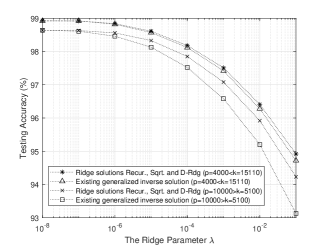
(a) MNIST dataset.

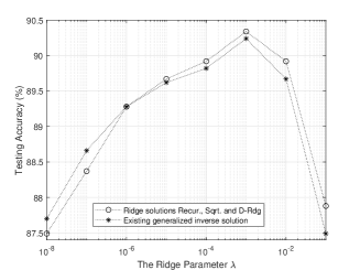
(b) NORB dataset.

Figure 1: The maximum testing accuracies achieved under different ridge parameters on MNIST and NORB datasets.

Regarding the simulations on the MNIST dataset for Tables ii@-vi@, the relevant networks and increments of inputs are as follows. The simulations for Table v@ of [7] are followed by those for Tables ii@ and iv@, where the network is constructed by $k=5100$ nodes including $10\times 10$ feature nodes and $5000$ enhancement nodes, and $p=10000>k$ training samples are added in each of the 5 update. In our simulations for Tables iii@ and v@, we construct the network by $k=15110$ nodes including $10\times 11$ feature nodes and $15000$ enhancement nodes, and add $p=4000<k$ training samples in each of the 5 update. Moreover, as Table vi@ in [7], Table vi@ gives the experimental results for the increment of inputs and nodes. In the simulations for Table vi@, we utilize 40000 training samples to train the initial network with $10\times 6$ feature nodes and $11000$ enhancement nodes, and in each of the 5 update, we increase 4000 inputs, and then increase 810 nodes including $10$ feature nodes, $300$ enhancement nodes only corresponding to the added feature nodes, and $500$ extra enhancement nodes.

Tables ii@ and iii@ give the testing accuracies  of the presented BLS algorithms, for the ridge parameter $\lambda={{10}^{-8}},{{10}^{-7}},\cdots,{{10}^{-1}}$. The simulations for Table ii@ show that Sqrt. and Recur. always achieve the same testing accuracy as D-Rdg when $\lambda\geq{{10}^{-7}}$ and $\lambda\geq{{10}^{-5}}$, respectively, and the simulations for Table iii@ show that Sqrt., Recur. and D-Rdg always achieve the same testing accuracy when $\lambda\geq{{10}^{-5}}$. Then for simplicity, the same testing accuracy achieved by multiple BLS algorithms is listed only once in Tables ii@ and iii@. As observed from Tables ii@ and iii@, both the proposed ridge solutions for BLS basically achieve the testing accuracy of the direct ridge solution, and improve the testing accuracy of the existing BLS when $\lambda\geq 10^{-7}$ in Table ii@ and $\lambda\geq 10^{-6}$ in Table iii@. The above-mentioned improvement becomes more significant as $\lambda$ is bigger.

Tables iv@ and v@ show the training time of the existing BLS and the proposed recursive and square-root algorithms, which is the average value of 500 simulations. In Tables iv@ and v@, the speedups are ${T_{existing}}/{T_{proposed}}$, i.e., the ratio between the training time of the existing BLS and that of the proposed algorithm. Table iv@ shows that when $p>k$, the speedups of Recur. and Sqrt. over Exst. in each additional training time are $1.99\sim 7.40$ and $3.22\sim 11.87$, respectively, and the speedups in total training time are $4.41$ and $6.92$, respectively. On the other hand, Table v@ shows that when $p<k$, the speedups of Recur. and Sqrt. over Exst. in each additional training time are $3.28\sim 4.37$ and $1.30\sim 1.75$, respectively, and the speedups in total training time are $2.80$ and $1.59$, respectively. Obviously both the proposed BLS algorithms significantly accelerate the existing BLS, while compared to the proposed recursive BLS, the proposed square-root BLS is faster when $p>k$, and is slower when $p<k$.

To increase inputs and nodes in our simulations for Table vii@, Exst. is applied with the original BLS on added nodes [7, Alg. 3], while both the proposed ridge solutions are applied with the efficient ridge solution for the BLS on added nodes [11] to obtain the complete ridge solution. As mentioned in the last subsection, when Recur. is applied with the efficient BLS in [11] that is based on the inverse Cholesky factor, (38) (i.e., ${{\mathbf{Q}}}={{\mathbf{F}}}{{\mathbf{F}}}^{T}$) is utilized to compute ${{\mathbf{F}}}$ from ${{\mathbf{Q}}}$ by the Cholesky factorization and compute ${{\mathbf{Q}}}$ from ${\mathbf{F}}$, which causes extra numerical errors. When $\lambda\leq 10^{-5}$, those extra numerical errors make ${{\mathbf{Q}}}$ no longer positive definite and causes the Cholesky factor of ${{\mathbf{Q}}}$ to be unavailable. Then Table vi@ has not given any testing accuracy for Recur. when $\lambda\leq 10^{-5}$. Moreover, Table vi@ shows that when $\lambda=10^{-4}$ or $\lambda=10^{-3}$, Recur. achieves worse testing accuracies than Sqrt., which can also be explained by the above-mentioned extra numerical errors. Thus we can conclude that when $\lambda$ is small and it is required to work with the efficient ridge solution based on the inverse Cholesky factor for the BLS on added nodes [11] for the increment of inputs and nodes, the proposed square-root BLS is more suitable than the proposed recursive BLS, to avoid the loss in testing accuracy caused by numerical errors.

Lastly, Table vii@ gives the testing accuracies of the presented BLS algorithms on the NORB dataset. In the simulations, we set the network as $k=15000$ nodes including $100\times 10$ feature nodes and $14000$ enhancement nodes, and add $p=1600<k$ training samples in each of the 5 updates, to increase the inputs from the initial 16300 to the final 24300. As shown in Table vii@, both the proposed ridge solutions for BLS basically achieve the testing accuracy of the direct ridge solution, and improve the testing accuracy of the existing BLS when $\lambda\geq 10^{-5}$. The above-mentioned improvement becomes more significant as $\lambda$ is bigger, as in Tables ii@ and iii@.

IV-C Analysis of the Maximum Testing Accuracies Achieved under Different Ridge Parameters

Fig. 1 shows the maximum testing accuracies achieved by the BLS algorithms under different ridge parameters on the MNIST and NORB datasets, which come from the accuracies in Tables ii@, iii@ and vii@. Since the ridge solutions Sqrt., Recur. and D-Rdg always achieve the same maximum testing accuracies, only the accuracies for the existing generalized inverse solution and the ridge solutions are listed in Fig. 1.

Tables ii@, iii@ and Fig. 1.a show that on the MNIST dataset, the existing generalized inverse solution and the ridge solutions achieve nearly the same maximum testing accuracy when $\lambda={{10}^{-8}}$. Specifically, Table iii@ shows that the ridge solutions and the existing BLS achieve the maximum testing accuracies of $98.93\%$ and $98.92\%$, respectively, and the former is a little better than the latter. On the other hand, Tables vii@ and Fig. 1.b show that on the NORB dataset, the ridge solutions and the existing BLS achieve the maximum testing accuracies of $90.34\%$ and $90.24\%$, respectively, when $\lambda={{10}^{-3}}$. Thus it can be concluded that compared with the existing generalized inverse solution, the proposed two ridge solutions achieve better maximum testing accuracies when the corresponding ridge parameter $\lambda$ is not too small, and achieve nearly the same maximum testing accuracy when the corresponding ridge parameter $\lambda$ is very small.

V Conclusion

To improve the existing BLS on added inputs, this paper proposes the recursive and square-root BLS algorithms, which utilize the inverse and inverse Cholesky factor of the Hermitian matrix in the ridge inverse, respectively, to update the ridge solution. The recursive BLS utilizes the matrix inversion lemma to update the inverse, while the square-root BLS updates the upper-triangular inverse Cholesky factor by multiplying it with an upper-triangular intermediate matrix. When the added $p$ inputs are more than the total $k$ nodes in the network, i.e., $p>k$, the inverse of a sum of matrices is utilized to take a smaller matrix inversion or inverse Cholesky factorization. For the distributed BLS with data-parallelism, we develop the parallel implementation of the square-root BLS, which is deduced by applying the parallel implementation of the inverse Cholesky factorization.

The existing BLS is based on the generalized inverse with the ridge regression, which assumes the ridge parameter $\lambda\to 0$ in the ridge inverse. When $\lambda\to 0$ is not satisfied, the numerical experiments on the MNIST and NORB datasets show that both the proposed ridge solutions improve the testing accuracy of the existing generalized inverse solution, and the improvement becomes more significant as $\lambda$ is bigger. Moreover, compared to the existing BLS, the proposed two ridge solutions achieve better and nearly the same maximum testing accuracies, respectively, when the corresponding ridge parameter does not satisfies and satisfies $\lambda\to 0$. On the MNIST dataset when $\lambda={{10}^{-8}}$, the maximum testing accuracies achieved by the proposed two ridge solutions and the existing BLS are $98.64\%$ in the case of $p>k$, and are $98.93\%$ and $98.92\%$ respectively in the case of $p<k$, while they are $90.34\%$ and $90.24\%$ respectively on the NORB dataset when $\lambda={{10}^{-3}}$.

With respect to the existing BLS, both the proposed BLS algorithms theoretically require less flops, and are significantly faster in the numerical experiments on the MNIST dataset. When $p>k$, the speedups in each additional training time of the proposed recursive and square-root BLS algorithms over the existing BLS are $1.99\sim 7.40$ and $3.22\sim 11.87$, respectively, and the speedups in total training time are $4.41$ and $6.92$, respectively. When $p<k$, the speedups in each additional training time of the recursive and square-root BLS algorithms over the existing BLS are $3.28\sim 4.37$ and $1.30\sim 1.75$, respectively, and the speedups in total training time are $2.80$ and $1.59$, respectively.

Compared to the recursive BLS, the square-root BLS requires less flops when $p>0.82k$, and requires more flops when $p<0.82k$. If nodes are inserted after each increment of inputs, both the proposed BLS algorithms are applied with the efficient ridge solution for the BLS on added nodes that is based on the inverse Cholesky factor, to obtain the complete ridge solution. In this case, the inverse of the Hermitian matrix utilized in the recursive BLS is Cholesky-factorized and then obtained again by multiplying the updated Cholesky factor with its transpose. The corresponding extra computations make the recursive BLS always require more flops than the square-root BLS, and cause the numerical errors. When $\lambda$ is small in the simulations, those numerical errors reduce the testing accuracy, or even make the recursive BLS unworkable. As a comparison, the square-root BLS does not need any extra computations and basically achieves the testing accuracy of the direct ridge solution, since it is based on the Cholesky factor just like the efficient ridge solution for the BLS on added nodes.

Appendix A The Derivation of (31)

Substitute (29) and (15) into (25) to obtain

$${{\bf{A}}_{\bar{l}+\bar{p}}^{\dagger}}=({{\mathbf{Q}}_{l}}-{{\mathbf{\tilde{B}}}}\mathbf{A}_{p}{{\mathbf{Q}}_{l}})\left[\begin{matrix}{\bf{A}}_{l}^{T}&{\bf{A}}_{p}^{T}\\ \end{matrix}\right]\\ =\left[\begin{matrix}{{\mathbf{Q}}_{\bar{l}}}{\bf{A}}_{\bar{l}}^{T}-{{\mathbf{\tilde{B}}}}\mathbf{A}_{\bar{p}}{{\mathbf{Q}}_{\bar{l}}}{\bf{A}}_{\bar{l}}^{T}&{{\mathbf{Q}}_{\bar{l}}}{\bf{A}}_{\bar{p}}^{T}-{{\mathbf{\tilde{B}}}}\mathbf{A}_{\bar{p}}{{\mathbf{Q}}_{\bar{l}}}{\bf{A}}_{\bar{p}}^{T}\\ \end{matrix}\right].$$ (61)

Then substitute (30) (i.e., ${{\mathbf{\tilde{B}}}}={{\mathbf{Q}}_{\bar{l}}}\mathbf{A}_{\bar{p}}^{T}{{(\mathbf{I}+\mathbf{A}_{\bar{p}}{{\mathbf{Q}}_{\bar{l}}}\mathbf{A}_{\bar{p}}^{T})}^{-1}}$) into the last entry in the right side of (61) to simplify it into

$${{\mathbf{Q}}_{\bar{l}}}{\bf{A}}_{\bar{p}}^{T}-{{\mathbf{\tilde{B}}}}\mathbf{A}_{\bar{p}}{{\mathbf{Q}}_{\bar{l}}}{\bf{A}}_{\bar{p}}^{T}$$

$$={{\mathbf{Q}}_{\bar{l}}}{\bf{A}}_{\bar{p}}^{T}-{{\mathbf{Q}}_{\bar{l}}}\mathbf{A}_{\bar{p}}^{T}{{(\mathbf{I}+\mathbf{A}_{\bar{p}}{{\mathbf{Q}}_{\bar{l}}}\mathbf{A}_{\bar{p}}^{T})}^{-1}}\mathbf{A}_{\bar{p}}{{\mathbf{Q}}_{\bar{l}}}{\bf{A}}_{\bar{p}}^{T}$$

$$={{\mathbf{Q}}_{\bar{l}}}{\bf{A}}_{\bar{p}}^{T}-{{\mathbf{Q}}_{\bar{l}}}\mathbf{A}_{\bar{p}}^{T}(\mathbf{I}-{{(\mathbf{I}+\mathbf{A}_{\bar{p}}{{\mathbf{Q}}_{\bar{l}}}\mathbf{A}_{\bar{p}}^{T})}^{-1}})$$

$$={{\mathbf{Q}}_{\bar{l}}}\mathbf{A}_{\bar{p}}^{T}{{(\mathbf{I}+\mathbf{A}_{\bar{p}}{{\mathbf{Q}}_{\bar{l}}}\mathbf{A}_{\bar{p}}^{T})}^{-1}}$$

$$={{\mathbf{\tilde{B}}}},$$ (62)

where (30) is applied to get the last row. Finally, we substitute (62) and (25) (i.e., ${{\bf{A}}_{\bar{l}}^{\dagger}}={{\mathbf{Q}}_{\bar{l}}}{{\bf{A}}_{\bar{l}}^{T}}$) into (61) to get (31).

Appendix B Parallel Implementation of Proposed Square-Root BLS Algorithm Based on Inverse Cholesky Factor for the Distributed BLS with Data-Parallelism

In this appendix, we use $K$ instead of $k$ to denote the total number of feature and enhancement nodes. We will describe the parallel implementations to compute ${\mathbf{F}}_{\bar{l}}\in{\Re^{K\times K}}$ by (38) and compute ${{\mathbf{F}}_{{\bar{l}}+\bar{p}}}\in{\Re^{K\times K}}$ by (41), (48), and (44), which include $K$ iterations. In the $k^{th}$ ($k=1,2,\cdots,K$) iteration, the $k\times k$ leading principal sub-matrices in the upper-triangular ${\mathbf{F}}_{\bar{l}}$ and ${{\mathbf{F}}_{{\bar{l}}+\bar{p}}}$ are computed.

B-A The Considered Distributed BLS with Data-Parallelism and the Corresponding Square-Root BLS

In the considered distributed BLS with data-parallelism, training samples are partitioned into $\tau$ workers. Worker $i$ ($i=1,2,\cdots,\tau$) possesses ${l_{i}}$ training samples that can be denoted as ${{\bf{A}}^{{l_{i}}}}\in{\Re^{l_{i}\times K}}$.

In the above-mentioned distributed BLS with data-parallelism, we can apply the proposed square-root BLS algorithm based on inverse Cholesky factor introduced in Algorithms 5 and 6. Accordingly, worker $i$ ($i=1,2,\cdots,\tau$) needs to compute the upper-triangular inverse Cholesky factor ${\mathbf{F}}^{{\tilde{l}}_{i}}\in{\Re^{K\times K}}$ satisfying

$${\mathbf{F}}^{{\tilde{l}}_{i}}({\mathbf{F}}^{{\tilde{l}}_{i}})^{T}={({{{({{\bf{A}}^{{{\tilde{l}}_{i}}}})^{T}}{{\bf{A}}^{{{\tilde{l}}_{i}}}}+\lambda\mathbf{I}}})^{-1}}$$ (63)

and the corresponding output weights ${\mathbf{W}}^{{\tilde{l}}_{i}}$ satisfying

$${\mathbf{W}}^{{\tilde{l}}_{i}}={\mathbf{F}}^{{\tilde{l}}_{i}}{({\mathbf{F}}^{{\tilde{l}}_{i}})^{T}}{({{\bf{A}}^{{{\tilde{l}}_{i}}}})^{T}}{{{\bf{Y}}^{{{\tilde{l}}_{i}}}}},$$ (64)

where

$${{\bf{A}}^{{{\tilde{l}}_{i}}}}=\left[{\begin{array}[]{*{20}{c}}{{{\bf{A}}^{{l_{1}}}}}&{{{\bf{A}}^{{l_{2}}}}}&\cdots&{{{\bf{A}}^{{l_{i}}}}}\end{array}}\right]$$ (65)

and ${{{\bf{Y}}^{{{\tilde{l}}_{i}}}}}=\left[{\begin{array}[]{*{20}{c}}{{{\bf{Y}}^{{l_{1}}}}}&{{{\bf{Y}}^{{l_{2}}}}}&\cdots&{{{\bf{Y}}^{{l_{i}}}}}\end{array}}\right]$ consist of

$${\tilde{l}}_{i}={l_{1}}+{l_{2}}+\cdots+{l_{i}}$$ (66)

training samples and labels (in workers $1,2,\cdots,i$), respectively. Notice that we can simply write (38) and (39) as the above (63) and (64), respectively.

To update the inverse Cholesky factor and the output weights incrementally without retraining the whole network from the beginning, worker $1$ computes the upper-triangular inverse Cholesky factor ${\mathbf{F}}^{{\tilde{l}}_{1}}$ and the corresponding output weights ${\mathbf{W}}^{{\tilde{l}}_{1}}$ by (63) and (64), respectively, and then transmits ${\mathbf{F}}^{{\tilde{l}}_{1}}$ and ${\mathbf{W}}^{{\tilde{l}}_{1}}$ to worker $2$. After receiving ${\mathbf{F}}^{{\tilde{l}}_{i-1}}$ and ${\mathbf{W}}^{{\tilde{l}}_{i-1}}$ from worker $i-1$, worker $i$ ($i=2,3,\cdots,\tau-1$) uses the $l_{i}$ training samples ${{\bf{A}}^{{l_{i}}}}$ in worker $i$ to obtain the upper-triangular inverse Cholesky factor ${\mathbf{V}}^{{\tilde{l}}_{i}}\in{\Re^{K\times K}}$ satisfying

$${\mathbf{V}}^{{\tilde{l}}_{i}}({\mathbf{V}}^{{\tilde{l}}_{i}})^{T}={{\left(\mathbf{I}+({\bf{E}}^{{\tilde{l}}_{i}})^{T}{\bf{E}}^{{\tilde{l}}_{i}}\right)}^{-1}}$$ (67)

with the $l_{i}\times K$ matrix

$${\bf{E}}^{{\tilde{l}}_{i}}={\bf{A}}^{{l}_{i}}{\mathbf{F}}^{{\tilde{l}}_{i-1}},$$ (68)

and updates ${\mathbf{F}}^{{\tilde{l}}_{i-1}}$ and ${\mathbf{W}}^{{\tilde{l}}_{i-1}}$ into

$${\mathbf{F}}^{{\tilde{l}}_{i}}={\mathbf{F}}^{{\tilde{l}}_{i-1}}{\mathbf{V}}^{{\tilde{l}}_{i}}$$ (69)

and

$${\mathbf{W}}^{{\tilde{l}}_{i}}={\mathbf{W}}^{{\tilde{l}}_{i-1}}+{\mathbf{F}}^{{\tilde{l}}_{i}}({\mathbf{F}}^{{\tilde{l}}_{i}})^{T}({\bf{A}}^{{l}_{i}})^{T}({{\bf{Y}}^{{l}_{i}}-{\bf{A}}^{{l}_{i}}{\mathbf{W}}^{{\tilde{l}}_{i-1}}}),$$ (70)

respectively. After computing ${\mathbf{F}}^{{\tilde{l}}_{i}}$ and ${\mathbf{W}}^{{\tilde{l}}_{i}}$ by (69) and (70), respectively, worker $i$ ($i=2,3,\cdots,\tau-1$) transmits ${\mathbf{F}}^{{\tilde{l}}_{i}}$ and ${\mathbf{W}}^{{\tilde{l}}_{i}}$ to worker $i+1$. Finally, worker $\tau$ uses the $l_{\tau}$ training samples ${{\bf{A}}^{{l_{\tau}}}}$ in worker $\tau$ to obtain the upper-triangular inverse Cholesky factor ${\mathbf{V}}^{{\tilde{l}}_{\tau}}$ by (68) and (67), and updates ${\mathbf{F}}^{{\tilde{l}}_{\tau-1}}$ and ${\mathbf{W}}^{{\tilde{l}}_{\tau-1}}$ into ${\mathbf{F}}^{{\tilde{l}}_{\tau}}$ and ${\mathbf{W}}^{{\tilde{l}}_{\tau}}$ by (69) and (70), respectively. Notice that we can compare (41) and (68) to deduce

$${\bf{E}}^{{\tilde{l}}_{2}}=\mathbf{S}^{T},$$ (71)

and then write (48), (44) and (49) as the above (67), (69) and (70), respectively.

B-B Several Variables for the Proposed Parallel Implementation

In this subsection, we introduce several variables that will be utilized in the proposed parallel implementation.

The first $k$ ($k\leq K$) columns of ${\bf{E}}^{{\tilde{l}}_{i}}$ defined by (68) can be denoted as

$${\bf{E}}_{|k}^{{\tilde{l}}_{i}}={\bf{E}}^{{\tilde{l}}_{i}}(:,1:k)={\bf{A}}^{{l}_{i}}(:,1:k){\mathbf{F}}_{k}^{{\tilde{l}}_{i-1}},$$ (72)

where ${\mathbf{F}}_{k}^{{\tilde{l}}_{i-1}}$ is the $k\times k$ leading principal sub-matrix in the upper-triangular ${\mathbf{F}}^{{\tilde{l}}_{i-1}}$, and the notations ${\bf{E}}^{{\tilde{l}}_{i}}(:,1:k)$ and ${\bf{A}}^{{l}_{i}}(:,1:k)$ follow the Matlab standard. Then let us utilize ${\bf{E}}_{|k}^{{\tilde{l}}_{i}}$ to define the $k\times k$ upper-triangular inverse Cholesky factor ${\mathbf{V}}_{k}^{{\tilde{l}}_{i}}$ satisfying

$${\mathbf{V}}_{k}^{{\tilde{l}}_{i}}({\mathbf{V}}_{k}^{{\tilde{l}}_{i}})^{T}={{\left(\mathbf{I}+({\bf{E}}_{|k}^{{\tilde{l}}_{i}})^{T}{\bf{E}}_{|k}^{{\tilde{l}}_{i}}\right)}^{-1}},$$ (73)

which can be written as

$${\mathbf{V}}_{k}^{{\tilde{l}}_{i}}({\mathbf{V}}_{k}^{{\tilde{l}}_{i}})^{T}=({\bf{R}}_{k}^{{\tilde{l}}_{i}})^{-1}$$ (74)

with

$${\bf{R}}_{k}^{{\tilde{l}}_{i}}=({\bf{E}}_{|k}^{{\tilde{l}}_{i}})^{T}{\bf{E}}_{|k}^{{\tilde{l}}_{i}}+{\bf{I}}.$$ (75)

The inverse Cholesky factorization [15] can be applied to update ${\mathbf{V}}_{k-1}^{{\tilde{l}}_{i}}$ and ${{{{\bf{F}}}_{k-1}^{{\tilde{l}}_{i}}}}$ into ${\mathbf{V}}_{k}^{{\tilde{l}}_{i}}$ and ${{\bf{F}}_{k}^{{\tilde{l}}_{i}}}$, respectively, by

$${\mathbf{V}}_{k}^{{\tilde{l}}_{i}}=\left[{\begin{array}[]{*{20}{c}}{\mathbf{V}}_{k-1}^{{\tilde{l}}_{i}}&{{\bf{\bar{v}}}_{k}^{{\tilde{l}}_{i}}}\\ {{\bf{0}}_{k-1}^{T}}&{{v_{kk}^{{\tilde{l}}_{i}}}}\end{array}}\right]=\left[{\begin{array}[]{*{20}{c}}{\left({\begin{array}[]{*{20}{c}}{\mathbf{V}}_{k-1}^{{\tilde{l}}_{i}}\\ {{\bf{0}}_{k-1}^{T}}\end{array}}\right)}&{{\bf{v}}_{k}^{{\tilde{l}}_{i}}}\end{array}}\right]$$ (76)

and

$${{\bf{F}}_{k}^{{\tilde{l}}_{i}}}=\left[{\begin{array}[]{*{20}{c}}{{{{\bf{F}}}_{k-1}^{{\tilde{l}}_{i}}}}&{{{\bf{\bar{f}}}}_{k}^{{\tilde{l}}_{i}}}\\ {{\bf{0}}_{k-1}^{T}}&{f_{kk}^{{\tilde{l}}_{i}}}\end{array}}\right]=\left[{\begin{array}[]{*{20}{c}}{\left({\begin{array}[]{*{20}{c}}{{{{\bf{F}}}_{k-1}^{{\tilde{l}}_{i}}}}\\ {{\bf{0}}_{k-1}^{T}}\end{array}}\right)}&{{{\bf{f}}}_{k}^{{\tilde{l}}_{i}}}\end{array}}\right],$$ (77)

where $k=2,3,\cdots,K$. In (76), ${{\bf{\bar{v}}}_{k}^{{\tilde{l}}_{i}}}$ can be computed by [15]

$${{\bf{\bar{v}}}_{k}^{{\tilde{l}}_{i}}}=-{{v_{kk}^{{\tilde{l}}_{i}}}}{\mathbf{V}}_{k-1}^{{\tilde{l}}_{i}}({\mathbf{V}}_{k-1}^{{\tilde{l}}_{i}})^{T}{\bf{R}}_{k}^{{\tilde{l}}_{i}}(1:k-1,k).$$ (78)

The parallel implementation of the inverse Cholesky factorization [11] can be applied to compute the $k^{th}$ column of ${{\bf{V}}_{k}^{{\tilde{l}}_{i}}}$ (i.e., ${{\bf{\bar{v}}}_{k}^{{\tilde{l}}_{i}}}$ and ${{v_{kk}^{{\tilde{l}}_{i}}}}$ in (76)) by

$${{v_{kk}^{{\tilde{l}}_{i}}}}=1/\sqrt{{{{\bf{\Xi}}}_{K-k+1}^{{\tilde{l}}_{i}}}(1,1)}$$ (79a)

$${{\bf{\bar{v}}}_{k}^{{\tilde{l}}_{i}}}={{v_{kk}^{{\tilde{l}}_{i}}}}{{\bf{\Pi}}_{k-1}^{{\tilde{l}}_{i}}}(:,1),$$ (79b)

where ${{\mathbf{\Pi}}_{k}}$ and ${{\mathbf{\Xi}}_{K-k}}$ are defined by [11]

$${{\mathbf{\Pi}}_{k}^{{\tilde{l}}_{i}}}=-{\mathbf{V}}_{k}^{{\tilde{l}}_{i}}({\mathbf{V}}_{k}^{{\tilde{l}}_{i}})^{T}({\bf{E}}_{|k}^{{\tilde{l}}_{i}})^{T}{\bf{\underline{E}}}_{K-k}^{{\tilde{l}}_{i}}$$ (80)

and

$${{\mathbf{\Xi}}_{K-k}^{{\tilde{l}}_{i}}}=({\bf{\underline{E}}}_{K-k}^{{\tilde{l}}_{i}})^{T}{\bf{\underline{E}}}_{K-k}^{{\tilde{l}}_{i}}+{\bf{I}}\\ -({\bf{\underline{E}}}_{K-k}^{{\tilde{l}}_{i}})^{T}{\bf{E}}_{|k}^{{\tilde{l}}_{i}}{\mathbf{V}}_{k}^{{\tilde{l}}_{i}}({\mathbf{V}}_{k}^{{\tilde{l}}_{i}})^{T}({\bf{E}}_{|k}^{{\tilde{l}}_{i}})^{T}{\bf{\underline{E}}}_{K-k}^{{\tilde{l}}_{i}},$$ (81)

respectively. In (80) and (81), ${\bf{\underline{E}}}_{K-k}^{{\tilde{l}}_{i}}$ denotes the last $K-k$ columns of the $l_{i}\times K$ matrix ${\bf{E}}^{{\tilde{l}}_{i}}$, and then from (68), we can deduce

$${\bf{\underline{E}}}_{K-k}^{{\tilde{l}}_{i}}={\bf{E}}^{{\tilde{l}}_{i}}(:,k+1:K)={\bf{A}}^{{l}_{i}}{\mathbf{F}}^{{\tilde{l}}_{i-1}}(:,k+1:K).$$ (82)

Substitute (72) and (82) into (80) and (81) to obtain

$${{\mathbf{\Pi}}_{k}^{{\tilde{l}}_{i}}}=-{\mathbf{V}}_{k}^{{\tilde{l}}_{i}}({\mathbf{V}}_{k}^{{\tilde{l}}_{i}})^{T}({\mathbf{F}}_{k}^{{\tilde{l}}_{i-1}})^{T}{\bf{A}}^{{l}_{i}}(:,1:k)^{T}{\bf{A}}^{{l}_{i}}\\ \times{\mathbf{F}}^{{\tilde{l}}_{i-1}}(:,k+1:K)$$ (83)

and

$${{\bf{\Xi}}_{K-k}^{{\tilde{l}}_{i}}}= {\mathbf{F}}^{{\tilde{l}}_{i-1}}(:,k+1:K)^{T}({\bf{A}}^{{l}_{i}})^{T}{\bf{A}}^{{l}_{i}}{\mathbf{F}}^{{\tilde{l}}_{i-1}}(:,k+1:K)+{\bf{I}}-$$

$${\mathbf{F}}^{{\tilde{l}}_{i-1}}(:,k+1:K)^{T}({\bf{A}}^{{l}_{i}})^{T}{\bf{A}}^{{l}_{i}}(:,1:k){\mathbf{F}}_{k}^{{\tilde{l}}_{i-1}}{\mathbf{V}}_{k}^{{\tilde{l}}_{i}}({\mathbf{V}}_{k}^{{\tilde{l}}_{i}})^{T}\times$$

$$({\mathbf{F}}_{k}^{{\tilde{l}}_{i-1}})^{T}{\bf{A}}^{{l}_{i}}{(:,1:k)^{T}}{\bf{A}}^{{l}_{i}}{\mathbf{F}}^{{\tilde{l}}_{i-1}}(:,k+1:K)$$

$$= {\mathbf{F}}^{{\tilde{l}}_{i-1}}(:,k+1:K)^{T}$$

$$\left(\begin{array}[]{l}{({{\bf{A}}^{{l_{i}}}})^{T}}{{\bf{A}}^{{l_{i}}}}-{({{\bf{A}}^{{l_{i}}}})^{T}}{{\bf{A}}^{{l_{i}}}}(:,1:k){\mathbf{F}}_{k}^{{\tilde{l}}_{i-1}}\\ \times{\mathbf{V}}_{k}^{{\tilde{l}}_{i}}({\mathbf{V}}_{k}^{{\tilde{l}}_{i}})^{T}({\mathbf{F}}_{k}^{{\tilde{l}}_{i-1}})^{T}{\bf{A}}^{{l}_{i}}{(:,1:k)^{T}}{\bf{A}}^{{l}_{i}}\end{array}\right)$$ (86)

$$\times{\mathbf{F}}^{{\tilde{l}}_{i-1}}(:,k+1:K)+{\bf{I}},$$ (87)

respectively. Then write (83) as

$${{\mathbf{\Pi}}_{k}^{{\tilde{l}}_{i}}}={{\mathbf{\tilde{\Pi}}}_{k}^{{\tilde{l}}_{i}}}{\mathbf{F}}^{{\tilde{l}}_{i-1}}(:,k+1:K)$$ (88)

where ${{\mathbf{\tilde{\Pi}}}_{k}^{{\tilde{l}}_{i}}}\in{\Re^{k\times K}}$ is defined by

$${{\mathbf{\tilde{\Pi}}}_{k}^{{\tilde{l}}_{i}}}=-{\mathbf{V}}_{k}^{{\tilde{l}}_{i}}({\mathbf{V}}_{k}^{{\tilde{l}}_{i}})^{T}({\mathbf{F}}_{k}^{{\tilde{l}}_{i-1}})^{T}{\bf{A}}^{{l}_{i}}(:,1:k)^{T}{\bf{A}}^{{l}_{i}},$$ (89)

and write (87) as

$${{\bf{\Xi}}_{K-k}^{{\tilde{l}}_{i}}}={\bf{I}}+{\mathbf{F}}^{{\tilde{l}}_{i-1}}(:,k+1:K)^{T}{{\bf{\tilde{\Xi}}}_{k}^{{\tilde{l}}_{i}}}{\mathbf{F}}^{{\tilde{l}}_{i-1}}(:,k+1:K)$$ (90)

where ${{\bf{\tilde{\Xi}}}_{k}}\in{\Re^{K\times K}}$ is defined by

$${{\bf{\tilde{\Xi}}}_{k}^{{\tilde{l}}_{i}}}={({{\bf{A}}^{{l_{i}}}})^{T}}{{\bf{A}}^{{l_{i}}}}-{({{\bf{A}}^{{l_{i}}}})^{T}}{{\bf{A}}^{{l_{i}}}}(:,1:k){\mathbf{F}}_{k}^{{\tilde{l}}_{i-1}}\times\\ {\mathbf{V}}_{k}^{{\tilde{l}}_{i}}({\mathbf{V}}_{k}^{{\tilde{l}}_{i}})^{T}({\mathbf{F}}_{k}^{{\tilde{l}}_{i-1}})^{T}{\bf{A}}^{{l}_{i}}{(:,1:k)^{T}}{\bf{A}}^{{l}_{i}}.$$ (91)

In what follows, ${{\mathbf{\tilde{\Pi}}}_{k}^{{\tilde{l}}_{i}}}$ defined by (89) and ${{\bf{\tilde{\Xi}}}_{k}}$ defined by (91) will be applied to develop the parallel implementation of the proposed square-root BLS algorithm based on inverse Cholesky factor.

B-C Parallel Implementation of Proposed Square-Root BLS Algorithm Based on Inverse Cholesky Factor

As described above, worker $1$ possesses ${l_{1}}$ training samples, i.e., ${{\bf{A}}^{{{\tilde{l}}_{1}}}}={{\bf{A}}^{{l_{1}}}}$, which are utilized to compute the upper-triangular inverse Cholesky factor ${\mathbf{F}}^{{\tilde{l}}_{1}}$ satisfying (63) with $i=1$. Worker $1$ can use the inverse Cholesky factorization [15] or the corresponding parallel implementation [11] to compute ${\mathbf{F}}^{{\tilde{l}}_{1}}$ in $K$ iterations. In the $k^{th}$ ($k=1,2,\cdots,K$) iteration, worker $1$ updates the $(k-1)\times(k-1)$ upper-triangular ${{{{\bf{F}}}_{k-1}^{{\tilde{l}}_{1}}}}$ into the $k\times k$ upper-triangular ${{\bf{F}}_{k}^{{\tilde{l}}_{1}}}$ by (77) with $i=1$, i.e.,

$${{\bf{F}}_{k}^{{\tilde{l}}_{1}}}=\left[{\begin{array}[]{*{20}{c}}{{{{\bf{F}}}_{k-1}^{{\tilde{l}}_{1}}}}&{{{\bf{\bar{f}}}}_{k}^{{\tilde{l}}_{1}}}\\ {{\bf{0}}_{k-1}^{T}}&{f_{kk}^{{\tilde{l}}_{1}}}\end{array}}\right]=\left[{\begin{array}[]{*{20}{c}}{\left({\begin{array}[]{*{20}{c}}{{{{\bf{F}}}_{k-1}^{{\tilde{l}}_{1}}}}\\ {{\bf{0}}_{k-1}^{T}}\end{array}}\right)}&{{{\bf{f}}}_{k}^{{\tilde{l}}_{1}}}\end{array}}\right].$$ (92)

It can be seen from (92) that worker $1$ only needs to compute ${\bf{f}}_{k}^{{\tilde{l}}_{1}}={\left[{\begin{array}[]{*{20}{c}}{{({{{\bf{\bar{f}}}}_{k}^{{\tilde{l}}_{1}}})^{T}}}&{f_{kk}^{{\tilde{l}}_{1}}}\end{array}}\right]^{T}}$, the $k^{th}$ column of ${{\bf{F}}_{k}^{{\tilde{l}}_{1}}}$ that contains the nonzero entries in the $k^{th}$ column of the upper-triangular ${\mathbf{F}}^{{\tilde{l}}_{1}}$. To improve the parallelization, worker $1$ can transmit ${\bf{f}}_{k}^{{\tilde{l}}_{1}}$ to worker $2$, after ${\bf{f}}_{k}^{{\tilde{l}}_{1}}$ is computed in the $k^{th}$ iteration. Accordingly, when worker $1$ is computing some of the columns $k+1,k+2,\cdots,K$ in ${\mathbf{F}}^{{\tilde{l}}_{1}}$, worker $2$ can utilize ${\bf{f}}_{k}^{{\tilde{l}}_{1}}$ to compute the $k^{th}$ column of the upper-triangular ${\mathbf{F}}^{{\tilde{l}}_{2}}$ in parallel, and does not need to wait till it receives the whole $K\times K$ matrix ${\mathbf{F}}^{{\tilde{l}}_{1}}$ from worker $1$.

Let us describe the general case for worker $i$ where $i=2,3,\cdots,\tau-1$. After receiving ${\bf{f}}_{k}^{{\tilde{l}}_{i-1}}$ from worker $i-1$, worker $i$ ($i=2,3,\cdots,\tau-1$) computes

$${\mathbf{\theta}}_{k}^{{\tilde{l}}_{i}}={\bf{\tilde{\Xi}}}_{k-1}^{{\tilde{l}}_{i}}(1:k,:)^{T}{\bf{f}}_{k}^{{\tilde{l}}_{i-1}}$$ (93a)

$${v_{kk}^{{\tilde{l}}_{i}}}=1/\sqrt{1+{\bf{\theta}}_{k}^{{\tilde{l}}_{i}}(1:k)^{T}{\bf{f}}_{k}^{{\tilde{l}}_{i-1}}}$$ (93b)

$${\bf{\bar{v}}}_{k}^{{\tilde{l}}_{i}}={v_{kk}^{{\tilde{l}}_{i}}}{{\bf{\tilde{\Pi}}}_{k-1}^{{\tilde{l}}_{i}}}(:,1:k){\bf{f}}_{k}^{{\tilde{l}}_{i-1}}$$ (93c)

$${{{\bf{\bar{f}}}}_{k}^{{\tilde{l}}_{i}}}={{{\bf{F}}_{k-1}^{{\tilde{l}}_{i}}}{\bf{\bar{v}}}_{k}^{{\tilde{l}}_{i}}+{v_{kk}^{{\tilde{l}}_{i}}}{{{\bf{\bar{f}}}}_{k}^{{\tilde{l}}_{i-1}}}}$$ (93d)

$${f_{kk}^{{\tilde{l}}_{i}}}={{f_{kk}^{{\tilde{l}}_{i-1}}}{v_{kk}^{{\tilde{l}}_{i}}}}$$ (93e)

$${{\bf{F}}_{k}^{{\tilde{l}}_{i}}}=\left[{\begin{array}[]{*{20}{c}}{{{{\bf{F}}}_{k-1}^{{\tilde{l}}_{i}}}}&{{{\bf{\bar{f}}}}_{k}^{{\tilde{l}}_{i}}}\\ {{\bf{0}}_{k-1}^{T}}&{f_{kk}^{{\tilde{l}}_{i}}}\end{array}}\right],$$ (93h)

and then transmits ${\bf{f}}_{k}^{{\tilde{l}}_{i}}={\left[{\begin{array}[]{*{20}{c}}{{({{{\bf{\bar{f}}}}_{k}^{{\tilde{l}}_{i}}})^{T}}}&{f_{kk}^{{\tilde{l}}_{i}}}\end{array}}\right]^{T}}$ to worker $i+1$. Notice that the above ${v_{kk}^{{\tilde{l}}_{i}}}$ and ${\bf{\bar{v}}}_{k}^{{\tilde{l}}_{i}}$ form the $k^{th}$ column of ${\bf{V}}_{k}^{{\tilde{l}}_{i}}$ by (76), while ${\bf{f}}_{k}^{{\tilde{l}}_{i}}={\left[{\begin{array}[]{*{20}{c}}{{({{{\bf{\bar{f}}}}_{k}^{{\tilde{l}}_{i}}})^{T}}}&{f_{kk}^{{\tilde{l}}_{i}}}\end{array}}\right]^{T}}$ forms the $k^{th}$ column of ${{\bf{F}}_{k}^{{\tilde{l}}_{i}}}$ by (93h), i.e., (77). Moreover, for the next iteration, worker $i$ updates ${{\bf{\tilde{\Pi}}}_{k-1}^{{\tilde{l}}_{i}}}$ and ${{\bf{\tilde{\Xi}}}_{k-1}^{{\tilde{l}}_{i}}}$ into ${{\bf{\tilde{\Pi}}}_{k}^{{\tilde{l}}_{i}}}$ and ${{\bf{\tilde{\Xi}}}_{k}^{{\tilde{l}}_{i}}}$, respectively, by

$${{\bf{\tilde{\Pi}}}_{k}^{{\tilde{l}}_{i}}}=\left[{\begin{array}[]{*{20}{c}}{{{\bf{\tilde{\Pi}}}_{k-1}^{{\tilde{l}}_{i}}}}\\ {{{\bf{0}}^{T}}}\end{array}}\right]-{v_{kk}^{{\tilde{l}}_{i}}}\left[{\begin{array}[]{*{20}{c}}{\bf{\bar{v}}}_{k}^{{\tilde{l}}_{i}}\\ {v_{kk}^{{\tilde{l}}_{i}}}\end{array}}\right]{({\mathbf{\theta}}_{k}^{{\tilde{l}}_{i}})^{T}}$$ (94e)

$${{\bf{\tilde{\Xi}}}_{k}^{{\tilde{l}}_{i}}}={{\bf{\tilde{\Xi}}}_{k-1}^{{\tilde{l}}_{i}}}-({v_{kk}^{{\tilde{l}}_{i}}})^{2}{\mathbf{\theta}}_{k}^{{\tilde{l}}_{i}}{({\mathbf{\theta}}_{k}^{{\tilde{l}}_{i}})^{T}}.$$ (94f)

When $i=\tau$, worker $\tau$ also computes (93h) and (94f), while it is no longer necessary for worker $\tau$ to transmit ${\bf{f}}_{k}^{{\tilde{l}}_{\tau}}$ to another worker. The above (93h) and (94f) will be deduced in the following subsections D and E, respectively.

In the $k^{th}$ ($k=1,2,\cdots,K$) iteration, worker $1$ computes ${\bf{f}}_{k}^{{\tilde{l}}_{1}}$ and transmits it to worker $2$, worker $i$ ($i=2,3,\cdots,\tau-1$) then computes (93h) to transmit ${\bf{f}}_{k}^{{\tilde{l}}_{i}}$ to worker $i+1$, and worker $\tau$ computes (93h) with $i=\tau$ to obtain ${\bf{f}}_{k}^{{\tilde{l}}_{\tau}}$ finally. It can be seen that the delay in worker $i$ ($i=2,3,\cdots,\tau$) mainly comes from  the computation of (93h). The dominant computational complexity of (93h) comes from (93a) , (93c) and (93d), which only require the flops (floating point operations) of $2k^{2}$, $2k^{2}$ and $k^{2}$, respectively. Thus it can be expected that the computation of (93h) will not cause too long a delay.

The proposed parallel implementation of square-root BLS is summarized in Algorithm 7, where ${\mathbf{F}}_{k}^{{\tilde{l}}_{i}}$ ($i=1,2,\cdots,\tau$) denotes the $k\times k$ leading principal sub-matrix in the upper-triangular ${\mathbf{F}}^{{\tilde{l}}_{i}}$, as mentioned above. Notice that in Algorithm 7, ${\bf{f}}_{k}^{{\tilde{l}}_{i}}$ ($i=1,2,\cdots,\tau$), the $k^{th}$ column of ${{\bf{F}}_{k}^{{\tilde{l}}_{i}}}$, contains the nonzero entries in the $k^{th}$ column of the upper-triangular ${\mathbf{F}}^{{\tilde{l}}_{i}}$.

Algorithm 7 : The Proposed Parallel Implementation of Square-Root BLS

1:${{\bf{A}}^{{l_{i}}}}\in{\Re^{l_{i}\times K}}$ ($i=1,2,\cdots,\tau$) in worker $i$, which denotes ${l_{i}}$ training samples stored in worker $i$;

2:The upper-triangular inverse Cholesky factor ${\mathbf{F}}^{{\tilde{l}}_{\tau}}\in{\Re^{K\times K}}$ satisfying ${\mathbf{F}}^{{\tilde{l}}_{\tau}}({\mathbf{F}}^{{\tilde{l}}_{\tau}})^{T}={({{{({{\bf{A}}^{{{\tilde{l}}_{\tau}}}})^{T}}{{\bf{A}}^{{{\tilde{l}}_{\tau}}}}+\lambda\mathbf{I}}})^{-1}}$ where ${{\bf{A}}^{{{\tilde{l}}_{\tau}}}}=\left[{\begin{array}[]{*{20}{c}}{{{\bf{A}}^{{l_{1}}}}}&{{{\bf{A}}^{{l_{2}}}}}&\cdots&{{{\bf{A}}^{{l_{\tau}}}}}\end{array}}\right]$;

3:for $k=1:K$ ($K$ is the size of ${\bf{R}}$) do

4:     Worker $1$ transmits ${\bf{f}}_{k}^{{\tilde{l}}_{1}}$ to worker $2$, where ${\bf{f}}_{k}^{{\tilde{l}}_{1}}$ is the $k^{th}$ column of ${{\bf{F}}_{k}^{{\tilde{l}}_{1}}}\in{\Re^{k\times k}}$; Then worker $1$ computes some of the columns $k+1,k+2,\cdots,K$ in ${\mathbf{F}}^{{\tilde{l}}_{1}}$;

5:     When worker $1$ is computing some of the columns $k+1,k+2,\cdots,K$ in ${\mathbf{F}}^{{\tilde{l}}_{1}}$, worker $2$ computes (93h) with $i=2$ in parallel to obtain ${\bf{f}}_{k}^{{\tilde{l}}_{2}}$ and form ${{\bf{F}}_{k}^{{\tilde{l}}_{2}}}\in{\Re^{k\times k}}$ after receiving ${\bf{f}}_{k}^{{\tilde{l}}_{1}}$ from worker $1$, and then transmits ${\bf{f}}_{k}^{{\tilde{l}}_{2}}$ to worker $3$. After ${\bf{f}}_{k}^{{\tilde{l}}_{2}}$ is computed, worker $2$ also computes (94f) to update ${{\bf{\tilde{\Pi}}}_{k-1}^{{\tilde{l}}_{2}}}$ and ${{\bf{\tilde{\Xi}}}_{k-1}^{{\tilde{l}}_{2}}}$ into ${{\bf{\tilde{\Pi}}}_{k}^{{\tilde{l}}_{2}}}$ and ${{\bf{\tilde{\Xi}}}_{k}^{{\tilde{l}}_{2}}}$, respectively, which is utilized in the $(k+1)^{th}$ iteration for worker $2$;

6:     $\cdots\cdots$

7:     When workers $i-1$ is computing (94f) to obtain ${{\bf{\tilde{\Pi}}}_{k}^{{\tilde{l}}_{i-1}}}$ and ${{\bf{\tilde{\Xi}}}_{k}^{{\tilde{l}}_{i-1}}}$, or computing some of the columns $k+1,k+2,\cdots,K$ in the upper-triangular ${\mathbf{F}}^{{\tilde{l}}_{i-1}}$, worker $i$ ($i=3,4,\cdots,\tau-1$) computes (93h) in parallel to obtain ${\bf{f}}_{k}^{{\tilde{l}}_{i}}$ and form ${{\bf{F}}_{k}^{{\tilde{l}}_{i}}}\in{\Re^{k\times k}}$ after receiving ${\bf{f}}_{k}^{{\tilde{l}}_{i-1}}$ from worker $i-1$, and then transmits ${\bf{f}}_{k}^{{\tilde{l}}_{i}}$ to worker $i+1$. After ${\bf{f}}_{k}^{{\tilde{l}}_{i}}$ is computed, worker $i$ also computes (94f) to update ${{\bf{\tilde{\Pi}}}_{k-1}^{{\tilde{l}}_{i}}}$ and ${{\bf{\tilde{\Xi}}}_{k-1}^{{\tilde{l}}_{i}}}$ into ${{\bf{\tilde{\Pi}}}_{k}^{{\tilde{l}}_{i}}}$ and ${{\bf{\tilde{\Xi}}}_{k}^{{\tilde{l}}_{i}}}$, respectively, which is utilized in the $(k+1)^{th}$ iteration for worker $i$.

8:     $\cdots\cdots$

9:     When workers $\tau-1$ is computing (94f) with $i=\tau-1$ to obtain ${{\bf{\tilde{\Pi}}}_{k}^{{\tilde{l}}_{\tau-1}}}$ and ${{\bf{\tilde{\Xi}}}_{k}^{{\tilde{l}}_{\tau-1}}}$, or computing some of the columns $k+1,k+2,\cdots,K$ in the upper-triangular ${\mathbf{F}}^{{\tilde{l}}_{\tau-1}}$, worker $\tau$ computes (93h) with $i=\tau$ in parallel to obtain ${\bf{f}}_{k}^{{\tilde{l}}_{\tau}}$ and form ${{\bf{F}}_{k}^{{\tilde{l}}_{\tau}}}\in{\Re^{k\times k}}$ after receiving ${\bf{f}}_{k}^{{\tilde{l}}_{\tau-1}}$ from worker $\tau-1$. After ${\bf{f}}_{k}^{{\tilde{l}}_{\tau}}$ is computed, worker $\tau$ computes (94f) to update ${{\bf{\tilde{\Pi}}}_{k-1}^{{\tilde{l}}_{\tau}}}$ and ${{\bf{\tilde{\Xi}}}_{k-1}^{{\tilde{l}}_{\tau}}}$ into ${{\bf{\tilde{\Pi}}}_{k}^{{\tilde{l}}_{\tau}}}$ and ${{\bf{\tilde{\Xi}}}_{k}^{{\tilde{l}}_{\tau}}}$, respectively, which is utilized in the $(k+1)^{th}$ iteration for worker $\tau$;

10:end for

11:${{\bf{F}}_{K}^{{\tilde{l}}_{\tau}}}={\mathbf{F}}^{{\tilde{l}}_{\tau}}\in{\Re^{K\times K}}$ is computed after $K$ iterations;

B-D The Derivation of (93h)

From ${\mathbf{\theta}}_{k}^{{\tilde{l}}_{i}}$ defined by (93a), we can deduce

$${\mathbf{\theta}}_{k}^{{\tilde{l}}_{i}}(1:k)={\bf{\tilde{\Xi}}}_{k-1}^{{\tilde{l}}_{i}}(1:k,1:k)^{T}{\bf{f}}_{k}^{{\tilde{l}}_{i-1}}.$$ (95)

To deduce (93b), substitute (90) with $k=k-1$ into (79a) to obtain

$${v_{kk}^{{\tilde{l}}_{i}}}=1/\sqrt{1+({\bf{f}}_{k}^{{\tilde{l}}_{i-1}})^{T}{{{\bf{\tilde{\Xi}}}}_{k-1}^{{\tilde{l}}_{i}}}(1:k,1:k){\bf{f}}_{k}^{{\tilde{l}}_{i-1}}},$$ (96)

into which substitute (95).

To deduce (93c), let us write (75) as

$${\bf{R}}_{k}^{{\tilde{l}}_{i}}(1:k-1,k)={\bf{E}}_{|k}^{{\tilde{l}}_{i}}(:,1:k-1)^{T}{\bf{E}}_{|k}^{{\tilde{l}}_{i}}(:,k).$$ (97)

From (72), we can deduce

$${\bf{E}}_{|k}^{{\tilde{l}}_{i}}(:,k)={\bf{A}}^{{l}_{i}}(:,1:k){\bf{f}}_{k}^{{\tilde{l}}_{i-1}}$$ (98)

and

$${\bf{E}}_{|k}^{{\tilde{l}}_{i}}(:,1:k-1) ={\bf{A}}^{{l}_{i}}(:,1:k){\mathbf{F}}_{k}^{{\tilde{l}}_{i-1}}(:,1:k-1)$$

$$={\bf{A}}^{{l}_{i}}(:,1:k){\left[{\begin{array}[]{*{20}{c}}{({\mathbf{F}}_{k-1}^{{\tilde{l}}_{i-1}})^{T}}&{{\bf{0}}_{k-1}}\end{array}}\right]^{T}}$$ (100)

$$={\bf{A}}^{{l}_{i}}(:,1:k-1){\mathbf{F}}_{k-1}^{{\tilde{l}}_{i-1}},$$ (101)

which are substituted into (97) to obtain

$${\bf{R}}_{k}^{{\tilde{l}}_{i}}(1:k-1,k)=\\ ({\mathbf{F}}_{k-1}^{{\tilde{l}}_{i-1}})^{T}{\bf{A}}^{{l}_{i}}(:,1:k-1)^{T}{\bf{A}}^{{l}_{i}}(:,1:k){\bf{f}}_{k}^{{\tilde{l}}_{i-1}}.$$ (102)

Then substitute (102) into (78) to obtain

$${{\bf{\bar{v}}}_{k}^{{\tilde{l}}_{i}}}=-{{v_{kk}^{{\tilde{l}}_{i}}}}{\mathbf{V}}_{k-1}^{{\tilde{l}}_{i}}({\mathbf{V}}_{k-1}^{{\tilde{l}}_{i}})^{T}\\ \times({\mathbf{F}}_{k-1}^{{\tilde{l}}_{i-1}})^{T}{\bf{A}}^{{l}_{i}}(:,1:k-1)^{T}{\bf{A}}^{{l}_{i}}(:,1:k){\bf{f}}_{k}^{{\tilde{l}}_{i-1}},$$ (103)

and write (89) as

$${{\bf{\tilde{\Pi}}}_{k-1}^{{\tilde{l}}_{i}}}(:,1:k)=-{\mathbf{V}}_{k-1}^{{\tilde{l}}_{i}}({\mathbf{V}}_{k-1}^{{\tilde{l}}_{i}})^{T}\\ \times({\mathbf{F}}_{k-1}^{{\tilde{l}}_{i-1}})^{T}{\bf{A}}^{{l}_{i}}(:,1:k-1)^{T}{\bf{A}}^{{l}_{i}}(:,1:k).$$ (104)

Finally, we substitute (104) into (103) to obtain (93c).

To deduce (93d) and (93e), substitute (77) and (76) into (69) to obtain

$${{{{\bf{F}}}_{k}^{{\tilde{l}}_{i}}}} ={\mathbf{F}}_{k}^{{\tilde{l}}_{i-1}}{\mathbf{V}}_{k}^{{\tilde{l}}_{i}}$$

$$=\left[{\begin{array}[]{*{20}{c}}{{{{\bf{F}}}_{k-1}^{{\tilde{l}}_{i-1}}}}&{{{\bf{\bar{f}}}}_{k}^{{\tilde{l}}_{i-1}}}\\ {{\bf{0}}_{k-1}^{T}}&{f_{kk}^{{\tilde{l}}_{i-1}}}\end{array}}\right]\left[{\begin{array}[]{*{20}{c}}{\mathbf{V}}_{k-1}^{{\tilde{l}}_{i}}&{{\bf{\bar{v}}}_{k}^{{\tilde{l}}_{i}}}\\ {{\bf{0}}_{k-1}^{T}}&{{v_{kk}^{{\tilde{l}}_{i}}}}\end{array}}\right]$$ (109)

$$=\left[{\begin{array}[]{*{20}{c}}{{{{\bf{F}}}_{k-1}^{{\tilde{l}}_{i-1}}}}{\mathbf{V}}_{k-1}^{{\tilde{l}}_{i}}&{{{\bf{F}}_{k-1}^{{\tilde{l}}_{i-1}}}{\bf{\bar{v}}}_{k}^{{\tilde{l}}_{i}}+{v_{kk}^{{\tilde{l}}_{i}}}{{{\bf{\bar{f}}}}_{k}^{{\tilde{l}}_{i-1}}}}\\ {{\bf{0}}_{k-1}^{T}}&{{f_{kk}^{{\tilde{l}}_{i-1}}}{v_{kk}^{{\tilde{l}}_{i}}}}\end{array}}\right],$$ (112)

which can be compared with (93h) (i.e., (77)) to deduce (93d) and (93e). Notice that it is not required to deduce (93h), since (93h) is the same as (77).

B-E The Derivation of (94f)

Define

$${{\bf{\Phi}}_{k}^{{\tilde{l}}_{i}}}=({\bf{A}}^{{l}_{i}})^{T}{\bf{A}}^{{l}_{i}}(:,1:k){\mathbf{F}}_{k}^{{\tilde{l}}_{i-1}}{\mathbf{V}}_{k}^{{\tilde{l}}_{i}},$$ (113)

which is substituted into (89) and (91) to obtain

$${{\mathbf{\tilde{\Pi}}}_{k}^{{\tilde{l}}_{i}}}=-{\mathbf{V}}_{k}^{{\tilde{l}}_{i}}({{\bf{\Phi}}_{k}^{{\tilde{l}}_{i}}})^{T}$$ (114)

and

$${{\bf{\tilde{\Xi}}}_{k}^{{\tilde{l}}_{i}}}=({\bf{A}}^{{l}_{i}})^{T}{\bf{A}}^{{l}_{i}}-{{\bf{\Phi}}_{k}^{{\tilde{l}}_{i}}}({{\bf{\Phi}}_{k}^{{\tilde{l}}_{i}}})^{T},$$ (115)

respectively. Then write (112) as ${\mathbf{F}}_{k}^{{\tilde{l}}_{i-1}}{\mathbf{V}}_{k}^{{\tilde{l}}_{i}}=\left[{\begin{array}[]{*{20}{c}}{{{{\bf{F}}}_{k-1}^{{\tilde{l}}_{i-1}}}}{\mathbf{V}}_{k-1}^{{\tilde{l}}_{i}}&{{{\bf{F}}_{k-1}^{{\tilde{l}}_{i-1}}}{\bf{\bar{v}}}_{k}^{{\tilde{l}}_{i}}+{v_{kk}^{{\tilde{l}}_{i}}}{{{\bf{\bar{f}}}}_{k}^{{\tilde{l}}_{i-1}}}}\\ {{\bf{0}}_{k-1}^{T}}&{{f_{kk}^{{\tilde{l}}_{i-1}}}{v_{kk}^{{\tilde{l}}_{i}}}}\end{array}}\right]$, which is substituted into (113) to obtain

$${{\bf{\Phi}}_{k}^{{\tilde{l}}_{i}}} =({\bf{A}}^{{l}_{i}})^{T}{\bf{A}}^{{l}_{i}}(:,1:k)\left[{\begin{array}[]{*{20}{c}}{{{{\bf{F}}}_{k-1}^{{\tilde{l}}_{i-1}}}}{\mathbf{V}}_{k-1}^{{\tilde{l}}_{i}}&{{{\bf{F}}_{k-1}^{{\tilde{l}}_{i-1}}}{\bf{\bar{v}}}_{k}^{{\tilde{l}}_{i}}+{v_{kk}^{{\tilde{l}}_{i}}}{{{\bf{\bar{f}}}}_{k}^{{\tilde{l}}_{i-1}}}}\\ {{\bf{0}}_{k-1}^{T}}&{{f_{kk}^{{\tilde{l}}_{i-1}}}{v_{kk}^{{\tilde{l}}_{i}}}}\end{array}}\right]$$ (118)

$$=\left[{\begin{array}[]{*{20}{c}}{({\bf{A}}^{{l}_{i}})^{T}{\bf{A}}^{{l}_{i}}(:,1:k-1){{{{\bf{F}}}_{k-1}^{{\tilde{l}}_{i-1}}}}{\mathbf{V}}_{k-1}^{{\tilde{l}}_{i}}}&{{\phi_{:k}^{{\tilde{l}}_{i}}}}\end{array}}\right]$$ (120)

$$=\left[{\begin{array}[]{*{20}{c}}{{\bf{\Phi}}_{k-1}^{{\tilde{l}}_{i}}}&{{\phi_{:k}^{{\tilde{l}}_{i}}}}\end{array}}\right]$$ (122)

with

$${\phi_{:k}^{{\tilde{l}}_{i}}} =({\bf{A}}^{{l}_{i}})^{T}{\bf{A}}^{{l}_{i}}(:,1:k){\left[{{{({{{\bf{F}}_{k-1}^{{\tilde{l}}_{i-1}}}{\bf{\bar{v}}}_{k}^{{\tilde{l}}_{i}}+{v_{kk}^{{\tilde{l}}_{i}}}{{{\bf{\bar{f}}}}_{k}^{{\tilde{l}}_{i-1}}}})}^{T}}}\;{{f_{kk}^{{\tilde{l}}_{i-1}}}{v_{kk}^{{\tilde{l}}_{i}}}}\right]^{T}}$$

$$=({\bf{A}}^{{l}_{i}})^{T}{\bf{A}}^{{l}_{i}}(:,1:k){v_{kk}^{{\tilde{l}}_{i}}}{\left[({{{\bf{\bar{f}}}}_{k}^{{\tilde{l}}_{i-1}}})^{T}\;{f_{kk}^{{\tilde{l}}_{i-1}}}\right]^{T}}$$

$$\quad\quad\quad\quad\quad\quad\quad+({\bf{A}}^{{l}_{i}})^{T}{\bf{A}}^{{l}_{i}}(:,1:k-1){{\bf{F}}_{k-1}^{{\tilde{l}}_{i-1}}}{\bf{\bar{v}}}_{k}^{{\tilde{l}}_{i}}$$

$$={v_{kk}^{{\tilde{l}}_{i}}}({\bf{A}}^{{l}_{i}})^{T}{\bf{A}}^{{l}_{i}}(:,1:k){{{\bf{f}}}_{k}^{{\tilde{l}}_{i-1}}}+$$

$$\quad\quad\quad\quad\quad\quad\quad+({\bf{A}}^{{l}_{i}})^{T}{\bf{A}}^{{l}_{i}}(:,1:k-1){{\bf{F}}_{k-1}^{{\tilde{l}}_{i-1}}}{\bf{\bar{v}}}_{k}^{{\tilde{l}}_{i}}.$$ (123)

To deduce (94e) that updates ${{\bf{\tilde{\Pi}}}_{k}^{{\tilde{l}}_{i}}}$, substitute (76) and (122) into (114) to obtain

$${{\bf{\tilde{\Pi}}}_{k}^{{\tilde{l}}_{i}}} =-\left[{\begin{array}[]{*{20}{c}}{\mathbf{V}}_{k-1}^{{\tilde{l}}_{i}}&{{\bf{\bar{v}}}_{k}^{{\tilde{l}}_{i}}}\\ {{\bf{0}}_{k-1}^{T}}&{{v_{kk}^{{\tilde{l}}_{i}}}}\end{array}}\right]\left[{\begin{array}[]{*{20}{c}}{{\bf{\Phi}}_{k-1}^{{\tilde{l}}_{i}}}&{{\phi_{:k}^{{\tilde{l}}_{i}}}}\end{array}}\right]^{T}$$ (127)

$$=\left[{\begin{array}[]{*{20}{c}}{-{\mathbf{V}}_{k-1}^{{\tilde{l}}_{i}}({{\bf{\Phi}}_{k-1}^{{\tilde{l}}_{i}}})^{T}-{{\bf{\bar{v}}}_{k}^{{\tilde{l}}_{i}}}({{\phi_{:k}^{{\tilde{l}}_{i}}}})^{T}}\\ {-{{v_{kk}^{{\tilde{l}}_{i}}}}({{\phi_{:k}^{{\tilde{l}}_{i}}}})^{T}}\end{array}}\right]$$ (130)

$$=\left[{\begin{array}[]{*{20}{c}}{{\bf{\tilde{\Pi}}}_{k-1}^{{\tilde{l}}_{i}}}\\ {{\bf{0}}_{k}^{T}}\end{array}}\right]-\left[{\begin{array}[]{*{20}{c}}{{\bf{\bar{v}}}_{k}^{{\tilde{l}}_{i}}}\\ {{v_{kk}^{{\tilde{l}}_{i}}}}\end{array}}\right]({{\phi_{:k}^{{\tilde{l}}_{i}}}})^{T}.$$ (135)

To deduce (94f) that updates ${{\bf{\tilde{\Xi}}}_{k}^{{\tilde{l}}_{i}}}$, substitute (122) into (115) to obtain

$${{\bf{\tilde{\Xi}}}_{k}^{{\tilde{l}}_{i}}} =({\bf{A}}^{{l}_{i}})^{T}{\bf{A}}^{{l}_{i}}-\left[{\begin{array}[]{*{20}{c}}{{\bf{\Phi}}_{k-1}^{{\tilde{l}}_{i}}}&{{\phi_{:k}^{{\tilde{l}}_{i}}}}\end{array}}\right]\left[{\begin{array}[]{*{20}{c}}{{\bf{\Phi}}_{k-1}^{{\tilde{l}}_{i}}}&{{\phi_{:k}^{{\tilde{l}}_{i}}}}\end{array}}\right]^{T}$$ (138)

$$=({\bf{A}}^{{l}_{i}})^{T}{\bf{A}}^{{l}_{i}}-{{\bf{\Phi}}_{k-1}^{{\tilde{l}}_{i}}}({{\bf{\Phi}}_{k-1}^{{\tilde{l}}_{i}}})^{T}-{{\phi_{:k}^{{\tilde{l}}_{i}}}}({{\phi_{:k}^{{\tilde{l}}_{i}}}})^{T}$$

$$={{\bf{\tilde{\Xi}}}_{k-1}^{{\tilde{l}}_{i}}}-{{\phi_{:k}^{{\tilde{l}}_{i}}}}({{\phi_{:k}^{{\tilde{l}}_{i}}}})^{T}.$$ (139)

Then it can be seen that we only need to verify

$${{v_{kk}^{{\tilde{l}}_{i}}}}{\mathbf{\theta}}_{k}^{{\tilde{l}}_{i}}={{\phi_{:k}^{{\tilde{l}}_{i}}}},$$ (140)

which is substituted into (135) and (139) to obtain (94e) and (94f), respectively.

In the end of this subsection, let us verify (140). Substitute (93a) into (140) to write

$${{v_{kk}^{{\tilde{l}}_{i}}}}{\mathbf{\theta}}_{k}^{{\tilde{l}}_{i}}={{v_{kk}^{{\tilde{l}}_{i}}}}{\bf{\tilde{\Xi}}}_{k-1}^{{\tilde{l}}_{i}}(1:k,:)^{T}{\bf{f}}_{k}^{{\tilde{l}}_{i-1}},$$ (141)

where ${\bf{\tilde{\Xi}}}_{k-1}^{{\tilde{l}}_{i}}(1:k,:)$ (i.e., the first $k$ rows of ${\bf{\tilde{\Xi}}}_{k-1}^{{\tilde{l}}_{i}}$) can be written as

$${\bf{\tilde{\Xi}}}_{k-1}^{{\tilde{l}}_{i}}(1:k,:)={{{\bf{A}}^{{l_{i}}}}(:,1:k)^{T}}{{\bf{A}}^{{l_{i}}}}-{\bf{A}}^{{l}_{i}}(:,1:k)^{T}{\bf{A}}^{{l}_{i}}(:,1:k-1)\\ \times{\mathbf{F}}_{k-1}^{{\tilde{l}}_{i-1}}{\mathbf{V}}_{k-1}^{{\tilde{l}}_{i}}({\mathbf{V}}_{k-1}^{{\tilde{l}}_{i}})^{T}({\mathbf{F}}_{k-1}^{{\tilde{l}}_{i-1}})^{T}{\bf{A}}^{{l}_{i}}{(:,1:k-1)^{T}}{{\bf{A}}^{{l}_{i}}}$$ (142)

by using (91). Then substitute (142) into (141) to obtain

$${{v_{kk}^{{\tilde{l}}_{i}}}}{\mathbf{\theta}}_{k}^{{\tilde{l}}_{i}}={{v_{kk}^{{\tilde{l}}_{i}}}}({{\bf{A}}^{{l_{i}}}})^{T}{{{\bf{A}}^{{l_{i}}}}(:,1:k)}{\bf{f}}_{k}^{{\tilde{l}}_{i-1}}-({{\bf{A}}^{{l_{i}}}})^{T}{\bf{A}}^{{l}_{i}}{(:,1:k-1)}{\mathbf{F}}_{k-1}^{{\tilde{l}}_{i-1}}\\ \times{{v_{kk}^{{\tilde{l}}_{i}}}}{\mathbf{V}}_{k-1}^{{\tilde{l}}_{i}}({\mathbf{V}}_{k-1}^{{\tilde{l}}_{i}})^{T}({\mathbf{F}}_{k-1}^{{\tilde{l}}_{i-1}})^{T}\\ \times{\bf{A}}^{{l}_{i}}(:,1:k-1)^{T}{\bf{A}}^{{l}_{i}}(:,1:k){\bf{f}}_{k}^{{\tilde{l}}_{i-1}}.$$ (143)

Finally, we substitute (103) into (143) to obtain

$${{v_{kk}^{{\tilde{l}}_{i}}}}{\mathbf{\theta}}_{k}^{{\tilde{l}}_{i}}={{v_{kk}^{{\tilde{l}}_{i}}}}({{\bf{A}}^{{l_{i}}}})^{T}{{{\bf{A}}^{{l_{i}}}}(:,1:k)}{\bf{f}}_{k}^{{\tilde{l}}_{i-1}}+({{\bf{A}}^{{l_{i}}}})^{T}{\bf{A}}^{{l}_{i}}{(:,1:k-1)}{\mathbf{F}}_{k-1}^{{\tilde{l}}_{i-1}}{{\bf{\bar{v}}}_{k}^{{\tilde{l}}_{i}}},$$

into which substitute (123) to obtain (140).

References

• [1] M. Leshno, V. Y. Lin, A. Pinkus, and S. Schocken, โ€œMultilayer feedforward networks with a nonpolynomial activation function can approximate any function,โ€ Neural Netw., vol. 6, no. 6, pp. 861-867.
• [2] Y.-H. Pao and Y. Takefuji, โ€œFunctional-link net computing: Theory, system architecture, and functionalities,โ€ Computer, vol. 25, no. 5, pp. 76-79, May 1992.
• [3] Y.-H. Pao, G.-H. Park, and D. J. Sobajic, โ€œLearning and generalization characteristics of the random vector functional-link net,โ€ Neurocomputing, vol. 6, no. 2, pp. 163-180, 1994.
• [4] Y. LeCun et al., โ€œHandwritten digit recognition with a back-propagation network,โ€ Proc. Neural Inf. Process. Syst. (NIPS), 1990, pp. 396-404.
• [5] J. S. Denker et al., โ€œNeural network recognizer for hand-written zip code digits,โ€ Advances in Neural Information Processing Systems, D. S. Touretzky, Ed. San Francisco, CA, USA: Morgan Kaufmann, 1989, pp. 323-331.
• [6] C. L. Philip Chen and J. Z. Wan, โ€œA rapid learning and dynamic stepwise updating algorithm for flat neural networks and the application to timeseries predictionโ€, IEEE Trans. Syst., Man, Cybern. B, Cybern., vol. 29, no. 1, pp. 62-72, Feb. 1999.
• [7] C. L. Philip Chen, and Z. Liu, โ€œBroad Learning System: An Effective and Efficient Incremental Learning System Without the Need for Deep Architectureโ€, IEEE Transactions on Neural Networks and Learning Systems, vol. 29, no. 1, Jan. 2018.
• [8] C. L. Philip Chen, Z. Liu, and S. Feng, โ€œUniversal Approximation Capability of Broad Learning System and Its Structural Variationsโ€, IEEE Transactions on Neural Networks and Learning Systems, vol. 30, no. 4, April 2019.
• [9] Donald W. Marquaridt, โ€œGeneralized Inverses, Ridge Regression, Biased Linear Estimation, and Nonlinear Estimationโ€, Technometrics, vol. 12, no. 3, Aug. 1970.
• [10] H. Zhu, Z. Liu, C. L. P. Chen and Y. Liang, โ€œAn Efficient Algorithm for the Incremental Broad Learning System by Inverse Cholesky Factorization of a Partitioned Matrixโ€, IEEE Access, vol. 9, pp. 19294-19303, 2021, doi: 10.1109/ACCESS.2021.3052102.
• [11] H. Zhu et al., โ€œTwo Ridge Solutions for the Incremental Broad Learning System on Added Nodesโ€, arXiv preprint arXiv:1911.04872v4 (12 Jan 2023).
• [12] H. V. Henderson and S. R. Searle, โ€œOn Deriving the Inverse of a Sum of Matricesโ€, SIAM Review, vol. 23, no. 1, January 1981.
• [13] H. Zhu et al., โ€œReducing the Computational Complexity of Pseudoinverse for the Incremental Broad Learning System on Added Inputsโ€, arXiv preprint arXiv:1910.07755(2019).
• [14] D.J. Tylavsky and G.R.L. Sohie, โ€œGeneralization of the matrix inversion lemmaโ€, Proceedings of the IEEE, pp. 1050-1052, vol. 74, no. 7, 1986.
• [15] H. Zhu, W. Chen, B. Li, and F. Gao, โ€œAn Improved Square-Root Algorithm for V-BLAST Based on Efficient Inverse Cholesky Factorizationโ€, IEEE Trans. Wireless Commun., vol. 10, no. 1, Jan. 2011.
• [16] J. Benesty, Y. Huang, and J. Chen, โ€œA fast recursive algorithm for optimum sequential signal detection in a BLAST systemโ€, IEEE Trans. Signal Process., pp. 1722-1730, July 2003.
• [17] https://ww2.mathworks.cn/help/matlab/ref/inv.html?lang=en
• [18] G. H. Golub and C. F. Van Loan, Matrix Computations, third ed. Baltimore, MD: Johns Hopkins Univ. Press, 1996.
• [19] Y. LeCun, L. Bottou, Y. Bengio, and P. Haffner, โ€œGradient-based learning applied to document recognitionโ€, Proc. IEEE, vol. 86, no. 11, pp. 2278-2324, Nov. 1998.
• [20] Y. LeCun, F. J. Huang, and L. Bottou, โ€œLearning methods for generic object recognition with invariance to pose and lightingโ€, Proc. IEEE Comput. Soc. Conf. Comput. Vis. Pattern Recognit. (CVPR), vol. 2, Jun. 2004, pp. II-94-II-104.
• [21] Joost Verbraeken, Matthijs Wolting, Jonathan Katzy, Jeroen Kloppenburg, Tim Verbelen, and Jan S. Rellermeyer, โ€œA Survey on Distributed Machine Learningโ€, ACM Computing Surveys, https://doi.org/10.1145/3377454.