Quantized Compressed Sensing by Rectified Linear Units

Abstract

This work is concerned with the problem of recovering high-dimensional signals $\mathbf{x}\in\mathbb{R}^{n}$ which belong to a convex set of low complexity from a small number of quantized measurements. We propose to estimate the signals via a convex program based on rectified linear units (ReLUs) for two different quantization schemes, namely one-bit and uniform multi-bit quantization. Assuming that the linear measurement process can be modelled by a sensing matrix with i.i.d. subgaussian rows, we obtain for both schemes near-optimal uniform reconstruction guarantees by adding well-designed noise to the linear measurements prior to the quantization step. In the one-bit case, we show that the program is robust against adversarial bit corruptions as well as additive noise on the linear measurements. Further, our analysis quantifies precisely how the rate-distortion relationship of the program changes depending on whether we seek reconstruction accuracies above or below the level of additive noise. The proofs rely on recent results by Dirksen and Mendelson on non-Gaussian hyperplane tessellations. Finally, we complement our theoretical analysis with numerical experiments which compare our method to other state-of-the-art methodologies.

Keywords: Compressed Sensing, Quantization, Rectified Linear Units, Hamming Distance

1 Introduction

The compressed sensing paradigm provides methods to infer accurate information about high-dimensional signals $\mathbf{x}\in\mathbb{R}^{n}$ from few linear measurements

$$\mathbf{y}=\mathbf{A}\mathbf{x}\in\mathbb{R}^{m},$$ (1.1)

where $\mathbf{A}\in\mathbb{R}^{m\times n}$ models a specific measurement process. The last decade showed that using prior knowledge on the unknown signal (e.g., sparsity) enables unique identification of $\mathbf{x}$ from $m\ll n$ measurements $\mathbf{y}$ via efficient recovery methods. In fact, under the assumption that $\mathbf{x}$ is $s$-sparse, meaning that at most $s$ entries are non-zero, unique recovery of $\mathbf{x}$ from $\mathbf{y}$ is possible, whenever we are given at least

$$m\geq Cs\log\left(\frac{en}{s}\right)$$ (1.2)

measurements. Here, and in the following, $C>0$ denotes an absolute constant. Starting with the works of [10, 17] compressed sensing has developed into a lively field of research which inspired new solutions for problems in various applied sciences [22, 33, 1]. We refer to [19] for a comprehensive discussion of compressed sensing and its applications.
Though the linear model (1.1) is powerful enough to encompass many import models of measurement processes, it is blind to the fact, that in real world scenarios the measurements have to be quantized to a finite number of bits before the signal reconstruction can be performed. The process of projecting the infinite precision measurements (captured as a real number) onto a finite alphabet $\mathcal{A}\subset\mathbb{R}$ is called quantization. Adapting (1.1) accordingly leads to the quantized compressed sensing model

$$\mathbf{q}=Q(\mathbf{A}\mathbf{x})\in\mathcal{A}^{m},$$ (1.3)

where the quantizer $Q\colon\mathbb{R}^{m}\rightarrow\mathcal{A}^{m}$ maps the linear measurements $\mathbf{A}\mathbf{x}$ to quantized measurements $\mathbf{q}$. Quantization in general leads to a loss of information which makes exact signal recovery impossible. Therefore, in the quantized compressed sensing model we are interested in designing quantizers $Q$ which permit efficient approximation of $\mathbf{x}$ from $\mathbf{q}$ using as few measurements as possible.
Although there exist more sophisticated quantization schemes, e.g., noise-shaping (for an overview see [9, 13]), our focus is on memoryless scalar quantization where the quantizer acts component-wise, i.e., $Q:\mathbb{R}\to\mathcal{A}$, and each linear measurement $\langle\mathbf{a}_{i},\mathbf{x}\rangle$ is quantized independently of all other measurements. In this context, we call $Q$ a $B$-bit quantizer if $|\mathcal{A}|=2^{B}$ and restrict ourselves to uniform quantization, which admits a rather simple structure. Let us mention that uniform quantizers approach optimality for increasing bit rates, cf. [20, p. 2332 et sqq.]). If $B$ is large, the measurement defect caused by $Q$ could be treated as noise and classical compressed sensing results would apply. However, in this case the reconstruction error cannot be smaller than the resolution of the quantizer. Assuming knowledge on the quantization process (which is most often the case in applications) this is suboptimal and does not use all available information [26]. Moreover, modern applications require as well a treatment of coarse quantization, i.e., $B$ is small, [5] and measurement devices become considerably cheaper in this regime, cf. [8].
In its coarsest form, $Q$ quantizes every measurement $\langle\mathbf{a}_{i},\mathbf{x}\rangle$ to one single bit $\mathbf{q}_{i}\in\{\pm 1\}$. Following [8], several works [6, 27, 34] examined one-bit quantization in compressed sensing and were able to derive recovery conditions which are asymptotically equivalent to (1.2). They could show for different efficient algorithms that it is possible to approximate $s$-sparse unit norm signals $\mathbf{x}$ up to reconstruction precision $\rho$ from $m\geq C(\rho)s\log(en/s)$ one-bit compressive measurements of the form

$$\mathbf{q}=\operatorname{sign}(\mathbf{A}\mathbf{x}),$$ (1.4)

where $C(\rho)>0$ is a constant only depending on $\rho$. Since (1.4) looses any scaling information, for this quantization scheme it is necessary to assume that the signals are normalized in order to prove approximation guarantees. To circumvent the normalization restriction, subsequent works [28, 24] added a random dither $\bm{\tau}\in\mathbb{R}^{m}$ to (1.4) leading to the dithered one-bit compressed sensing model

$$\mathbf{q}=\operatorname{sign}(\mathbf{A}\mathbf{x}+\bm{\tau})$$ (1.5)

allowing signal approximation for general $s$-sparse signals. The origin of these dithering techniques goes back to the work [38] where dithering was introduced in order to remove artefacts from quantized pictures (see also [20]).

In comparison to unquantized compressed sensing where measurement noise is usually modelled as a bounded additive perturbation of $\mathbf{y}$ in (1.1), one typically considers two different types of measurement noise in the one-bit models $\eqref{eq:OneBitCS}$ and $\eqref{eq:OneBitCSdithered}$: additive (statistical) noise $\bm{\nu}\in\mathbb{R}^{m}$ disturbing the linear measurements before quantization and (adversarial) bit-flips, cf. [27, 35, 15]. For an extended discussion on the goals of quantized compressed sensing and its particular challenges, we refer the reader to the recent survey [13]. In this work, we consider both additive statistical noise as well as adversarial bit corruptions. More specifically, we aim to recover vectors $\mathbf{x}$ from adversarially corrupted one-bit measurements $\mathbf{q}_{\text{corr}}$ which satisfy

$$d_{H}(\mathbf{q}_{\text{corr}},q(\mathbf{x}))\leq\beta m,$$ (1.6)

where the Hamming distance $d_{H}(\mathbf{z},\mathbf{z}^{\prime})=|\{i\colon z_{i}\neq z_{i}^{\prime}\}|$ counts the number of entries where $\mathbf{q}_{\text{corr}}$ differs from $q(\mathbf{x})=\operatorname{sign}(\mathbf{A}\mathbf{x}+\bm{\nu}+\bm{\tau})$, and $\bm{\nu}\in\mathbb{R}^{m}$ models subgaussian additive noise.
Finally, let us mention that we do not exclusively focus our work on sparse signals, but allow for general compact and convex sets $\mathcal{T}\subset\mathbb{R}^{n}$ as a prior. To obtain sparse reconstruction results, $\mathcal{T}$ would be chosen as a properly scaled $\ell_{1}$-ball and we will later on allude to sparse reconstruction as benchmark and sanity check.

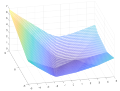
(a) The functional $\mathcal{L}_{\mathbf{q}}$.

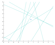
(b) The underlying tessellation and $\mathbf{x}$.

Figure 1: Example of $\mathcal{L}_{\mathbf{q}}$ and its underlying tessellation in $\mathbb{R}^{2}$. The parameters are chosen as $\mathbf{x}=(0.5,0.5)^{T}$, $m=10$, $\tau_{i}\sim\text{Unif}([-0.5,0.5])$, and $\mathbf{q}=\operatorname{sign}(\mathbf{A}\mathbf{x}+\bm{\tau})$. In (a) one can clearly see the Hamming structure from (b) encoded in $\mathcal{L}_{\mathbf{q}}$.

1.1 Contribution

(i) We propose to estimate vectors $\mathbf{x}\in\mathcal{T}\subset\mathbb{R}^{n}$ from $\mathbf{q}_{\text{corr}}$ in (1.6) by minimizing the convex functional

$$\mathcal{L}_{\mathbf{q}_{\text{corr}}}(\mathbf{z}):=\frac{1}{m}\sum_{i=1}^{m}\left[-(q_{\text{corr}})_{i}(\langle\mathbf{a}_{i},\mathbf{z}\rangle+\tau_{i})\right]_{+}\;,$$ (1.7)

where $\left[x\right]_{+}=\max\{x,0\}$ denotes the rectified linear unit (ReLU), cf. Figure 1. This amounts to solving the program

$$\min_{\mathbf{z}\in\mathbb{R}^{n}}\mathcal{L}_{\mathbf{q}_{\text{corr}}}(\mathbf{z})\quad\text{subject to}\quad\mathbf{z}\in\mathcal{T}, P_{\mathbf{q}_{\text{corr}}}$$ ()

which is a convex program whenever the set $\mathcal{T}$ is a convex subset of $\mathbb{R}^{n}$. From a geometric point of view, the functional $\mathcal{L}_{\mathbf{q}_{\text{corr}}}$ is a convex proxy for the Hamming distance based function $\mathbf{z}\mapsto d_{H}(\mathbf{q}_{\text{corr}},\operatorname{sign}(\mathbf{A}\mathbf{z}+\bm{\tau}))$ and exhibits intuitive relations to established approaches in recent literature, cf. Section (1.4) below. By designing the dither $\bm{\tau}$ to be uniformly distributed in $[-\lambda,\lambda]^{m}$ for a large enough parameter $\lambda>0$, we provide in Theorem 1 near-optimal robust uniform reconstruction guarantees for ($P_{\mathbf{q}_{\text{corr}}}$) under the assumption of i.i.d. subgaussian measurement vectors $\mathbf{a}_{i}$. These guarantees match state-of-the art results established in [15] for reconstruction accuracies below the noise level $\left\|\nu\right\|_{L^{2}}$, and improve them for accuracies above.

(ii) We extend the estimation scheme proposed in (1.7) and ($P_{\mathbf{q}_{\text{corr}}}$) to a memoryless uniform multi-bit quantization model with refinement level $\Delta>0$, which is the worst-case distortion when $Q$ is applied on a bounded domain. This leads to a modified version of (1.7) and ($P_{\mathbf{q}_{\text{corr}}}$), see Section 2.2 for details. By choosing the dither $\bm{\tau}$ to be uniformly distributed in $[-\Delta,\Delta]^{m}$, we derive uniform reconstruction guarantees, see Theorem 3, which exhibit two, for multi-bit quantization problems characteristic regimes: if we ask for approximation accuracies above the refinement level $\Delta$, the established guarantee resembles results typical for noisy unquantized compressed sensing models (1.1). If we ask for accuracies below the refinement level, additional oversampling becomes necessary and the result bears resemblance to the one-bit case. To keep the presentation concise, we do not consider noise on the measurements for multi-bit quantization (though possible as is evident from the one-bit setting; the interested reader is referred to the comments following Theorem 3). Let us emphasize that both in the one-bit and multi-bit setting our reconstruction guarantees are near-optimal in the context of memory-less scalar quantization (see the discussion on optimality below Theorem 3 and [16, Section 5]). Note that adaptive quantization schemes [4] allow better rates. Due to energy consumption and dependencies between single measurements, however, those systems can be of limited use in modern applications like Massive MIMO [21].

Numerical experiments illustrate the performance of ($P_{\mathbf{q}_{\text{corr}}}$) in both settings. While the idea of using half sided $\ell_{1}$- and $\ell_{2}$-norms is not new for quantized compressed sensing and appeared before in [27, 7], to the best of our knowledge, this is the first work unifying one- and multi-bit quantization for compressed sensing in a single tractable program and analysis.

1.2 Related Work (One-Bit)

Let us recap the state of the art in memoryless scalar quantized compressed sensing before presenting our main results in full detail. Recent results treat measurement noise as well as general signal sets $\mathcal{T}\subset\mathbb{R}^{n}$. In this context, the Gaussian width is a natural complexity parameter which has proven to accurately capture the effective size of signal sets in many problems from signal processing. The Gaussian width of a set $\mathcal{T}\subset\mathbb{R}^{n}$ is defined as

$$w_{*}(\mathcal{T}):=\mathbb{E}\sup_{\mathbf{x}\in\mathcal{T}}|\langle\mathbf{g},\mathbf{x}\rangle|,$$

where $\mathbf{g}\in\mathbb{R}^{n}$ is a standard Gaussian random vector. As a rule of thumb one may say that the squared Gaussian width corresponds to the information theoretic intrinsic complexity of $\mathcal{T}$. Further, the Gaussian width plays an important role in high-dimensional probability, statistics and geometry. For more information on its role in problems from signal recovery, the reader is referred to [35, 41, 3].

The first result on robust recovery from one-bit quantized compressed sensing measurements using a tractable recovery algorithm appeared in [35] for an un-dithered model. The authors showed that if $\mathbf{A}$ is an $m\times n$ Gaussian matrix and $m\gtrsim\rho^{-6}w_{*}(\mathcal{T})^{2}$, for $\rho>0$, then, with high probability, every $\mathbf{x}\in\mathcal{T}\cap\mathcal{S}^{n-1}$ is recovered from $\mathbf{q}_{\text{corr}}$ as in (1.6), for $\beta>0$ and $q(\mathbf{x})$ as in (1.4), by any solution $\mathbf{x}^{\#}$ of the program

$$\max_{\mathbf{z}\in\mathcal{T}}\frac{1}{m}\sum_{i=1}^{m}(q_{\text{corr}})_{i}\langle\mathbf{a}_{i},\mathbf{z}\rangle$$ (1.8)

up to error $\|\mathbf{x}-\mathbf{x}^{\#}\|_{2}^{2}=\mathcal{O}(\rho\sqrt{\log(e/\rho)})+\mathcal{O}(\beta\sqrt{\log(e/\beta)})$. If $\mathcal{T}$ is convex, then the program (1.8) is convex as well. While the dependence on the intrinsic complexity of $\mathcal{T}$ is optimal in this result, the dependence on the approximation accuracy $\rho$ is highly suboptimal. In [2] it was shown that the program (1.8) is even capable of estimating a fixed signal $\mathbf{x}\in\mathcal{S}^{n-1}$ from one-bit measurements (1.4) if $\mathbf{A}$ is a subgaussian measurement matrix, provided that the $\ell_{\infty}$-norm of $\mathbf{x}$ is small enough. Due to the un-dithered measurement set-up, however, the additional assumption on $\mathbf{x}$ is necessary. On the one hand, the result shows that, apart from very sparse vectors, the program (1.8) still succeeds at recovering signal vectors from one-bit subgaussian measurements. On the other hand, the vectors have to be normalized, the result is non-uniform, and the dependence on the approximation accuracy $\rho$ is still suboptimal.

The follow-up work [15] massively improved on all of these points by considering dithered one-bit measurements as in (1.5) and adding a regularizing term to (1.8). For the resulting program

$$\max_{\mathbf{z}\in\mathcal{T}}\frac{1}{m}\left(\sum_{i=1}^{m}(q_{\text{corr}})_{i}\langle\mathbf{a}_{i},\mathbf{z}\rangle\right)-\frac{1}{2\lambda}\|\mathbf{z}\|_{2}^{2}$$ (1.9)

the authors showed the following robust reconstruction guarantee (ignoring log-factors): if $\bm{\tau}\in[-\lambda,\lambda]^{m}$ is uniformly distributed for a sufficiently large parameter $\lambda$, then the convex program (1.9) is capable of uniformly recovering all signals $\mathbf{x}\in\mathcal{T}\subset B^{n}_{2}$ from corrupted one-bit measurements $\mathbf{q}_{\text{corr}}$ as in (1.6) up to accuracy $\rho$ provided that $\left\|\nu\right\|_{L^{2}}\lesssim 1$, $\beta\lesssim\rho$ and the number of measurements satisfies

$$m\gtrsim\rho^{-4}w_{*}((\mathcal{T}-\mathcal{T})\cap\rho B^{n}_{2})^{2}+\rho^{-2}\log\mathcal{N}(\mathcal{T},\rho/\sqrt{\log(c/\rho)}).$$ (1.10)

Here $w_{*}((\mathcal{T}-\mathcal{T})\cap\rho B^{n}_{2})^{2}$ is a localized variant of the Gaussian width and $\mathcal{N}(\mathcal{T},\varepsilon)$ denotes the $\varepsilon$-covering number of $\mathcal{T}$ with respect to the Euclidean distance, i.e., the smallest number of Euclidean balls with radius $\varepsilon$ that are needed to cover $\mathcal{T}$. Ignoring log-factors, Sudakov’s inequality shows that condition (1.10) is already satisfied if $m\gtrsim\rho^{-4}w_{*}(\mathcal{T})^{2}$. This massively improves on earlier uniform reconstruction guarantees. Moreover, the result shows that by using dithering in the measurement process there is no need of imposing additional structural assumptions on the signal vectors (such as a small $\ell_{\infty}$-norm). However, the result has a drawback as well: it is not sensitive to the magnitude of the additive noise on the linear measurements as long as $\left\|\nu\right\|_{L^{2}}\leq R$. In particular, $\left\|\nu\right\|_{L^{2}}\approx 0$ and $\left\|\nu\right\|_{L^{2}}\approx R$ lead to the same reconstruction guarantees. This suboptimal performance in a low-noise setting is clearly observed experimentally, cf. Section 4.

1.3 Related Work (Multi-Bit)

Compared to the extensive theoretical studies on recovery algorithms in one-bit compressed sensing for memoryless scalar quantization, fewer comprehensive results exist for finer quantization. One has to understand that a multi-bit quantizer $Q$ with refinement level $\Delta>0$ leads in compressed sensing to two very different recovery regimes: if the local complexity of $\mathcal{T}$ behaves similar to their global complexity, i.e., $w_{*}((\mathcal{T}-\mathcal{T})\cap\rho B_{2}^{n})\simeq\rho w_{*}(\mathcal{T})$, the sufficient number of measurements to obtain an approximation error $\rho\gtrsim\Delta$ does not depend on $\rho$ (high quantizer resolution $\leftrightarrow$ un-quantized compressed sensing regime); to obtain smaller approximation errors, the number of measurements must behave similar to the one-bit case (low quantizer resolution $\leftrightarrow$ one-bit compressed sensing regime). As [30] shows, it is favorable to increase the bit-depth per measurement if high-accuracy is sought, if the expected noise-level is low, or if the number of measurements underlies stronger restrictions than the number of bits. Though several articles numerically examined recovery algorithms for multi-bit quantized compressed sensing [25, 26, 39], to the best of our knowledge no comprehensive theoretical guarantees covering both regimes were derived for tractable algorithms apart from [14, 32]. Therein Consistent Basis Pursuit (CBP) is theoretically examined, but the analysis is restricted to signal sets corresponding to atomic norm balls and the obtained guarantees have with $m\gtrsim\Delta^{-2}\rho^{-4}w_{\ast}(\mathcal{T})^{2}$ a far worse error dependence than the one-bit results in [15] would suggest. More important, CBP becomes infeasible under noise on the measurements. The work [24] examines consistent reconstruction which is not tractable in general. The tractable Basis Pursuit De-Noising (BPDN) [11, 26] only covers the high quantizer resolution regime, i.e., the achievable approximation error $\rho$ is lower bounded by $\Delta$. The work [42] examines an equivalent variant of (1.9) for multi-bit quantization but only reflects the low quantizer resolution regime. For small $\Delta$, the measurement requirements become suboptimal. Moreover, the requirement $m\gtrsim\rho^{-16}w_{\ast}(\mathcal{T})^{2}$ for general bounded, convex, and symmetric sets is rather pessimistic. Last but not least, [36, 37] are restricted to Gaussian measurements and treat a more general non-linear adaption of (1.1) which covers (1.3) as a special case but only leads to non-uniform recovery guarantees.

1.4 A first intuition

Let us compare ($P_{\mathbf{q}_{\text{corr}}}$) to the state-of-the-art methods for robust one-bit quantized compressed sensing presented above. Though at first sight, ($P_{\mathbf{q}_{\text{corr}}}$) appears to be closely related to (1.8) and (1.9), the motivation for the program and its geometric meaning is fundamentally different. Both (1.8) and (1.9) aim at maximizing the alignment of quantized and unquantized measurements while ignoring the concrete geometry defined by the quantization cells. As already mentioned in [29, 23] one can reformulate (1.8) as

$$\min_{\mathbf{z}\in\mathcal{T}} \left(\sum_{i\colon(q_{\text{corr}})_{i}\neq\operatorname{sign}(\langle\mathbf{a}_{i},\mathbf{z}\rangle)}\|\mathbf{a}_{i}\|_{2}\left\|\mathbf{z}-\mathbb{P}_{H_{\mathbf{a}_{i}}}\mathbf{z}\right\|_{2}\;-\sum_{i\colon(q_{\text{corr}})_{i}=\operatorname{sign}(\langle\mathbf{a}_{i},\mathbf{z}\rangle)}\|\mathbf{a}_{i}\|_{2}\left\|\mathbf{z}-\mathbb{P}_{H_{\mathbf{a}_{i}}}\mathbf{z}\right\|_{2}\right),$$ (1.11)

where $\mathbb{P}_{H_{\mathbf{a}_{i}}}$ denotes the orthogonal projection onto the hyperplane defined by $\mathbf{a}_{i}$. Consequently, maximizing the alignment in (1.8) corresponds to punishing wrong measurements $\operatorname{sign}(\langle\mathbf{a}_{i},\mathbf{z}\rangle)\neq(q_{\text{corr}})_{i}$ of a point $\mathbf{z}\in\mathcal{T}$ by its Euclidean distance to the corresponding hyperplane $H_{\mathbf{a}_{i}}$ and rewarding correct measurements by the same amount. If the measurements are trustworthy, i.e., $(q_{\text{corr}})_{i}=q_{i}=\operatorname{sign}(\langle\mathbf{a}_{i},\mathbf{x}\rangle)$ for all $i\in[m]$, the rewarding term unnecessarily allows hyperplanes $H_{\mathbf{a}_{i}}$ not separating $\mathbf{z}$ and $\mathbf{x}$ to influence the penalization in (1.8) and leads to worse approximation. Having (1.11) in mind, the regularizer in (1.9) might be interpreted as a compensation for the rewarding part. In contrast, the ReLU-formulation in ($P_{\mathbf{q}_{\text{corr}}}$) completely drops the rewarding part of (1.11) and resembles a continuous proxy of the Hamming-distance on the quantization cell structure (see Figure 1). In particular, in the noiseless case, that is, in the case where $(q_{\text{corr}})_{i}=\operatorname{sign}(\langle\mathbf{a}_{i},\mathbf{x}\rangle+\tau_{i})$ for all $i\in[m]$, we have $\mathcal{L}_{\mathbf{q}_{\text{corr}}}(\mathbf{x})=0$ and therefore any solution $\mathbf{x}^{\#}$ to ($P_{\mathbf{q}_{\text{corr}}}$) has to satisfy $\mathcal{L}_{\mathbf{q}_{\text{corr}}}(\mathbf{x}^{\#})=0$ as well. Since this is equivalent to $\operatorname{sign}(\langle\mathbf{a}_{i},\mathbf{x}\rangle+\tau_{i})=\operatorname{sign}(\langle\mathbf{a}_{i},\mathbf{x}^{\#}\rangle+\tau_{i})$ for all $i\in[m]$, we see that in the noiseless case minimizing ($P_{\mathbf{q}_{\text{corr}}}$) forces the reconstructed signal to lie on the correct sides of all shifted hyperplanes. Note that (1.9) completely neglects the knowledge about the hyperplane shifts and thus simply treats the dither as additive noise.

1.5 Outline

We state and explain the main results of the paper, Theorem 1 & 3, in Section 2. The proofs of both results are then provided in Section 3. Section 4 supports our theoretical findings by numerically comparing ($P_{\mathbf{q}_{\text{corr}}}$) to different competing recovery schemes in both the one-bit and multi-bit setting. The proofs of some technical tools are deferred to the Appendix.

1.6 Notation

We will use the following notation throughout the paper:

1. For $k\in\mathbb{N}$ we set $[k]:=\{1,\ldots,k\}$. Matrices and vectors are denoted by upper- and lowercase boldface letters, respectively.

2. For $\mathbf{x}\in\mathbb{R}^{n}$ we set $\|\mathbf{x}\|_{0}:=|\{i\in[n]\;:\;x_{i}\neq 0\}|$. A vector $\mathbf{x}\in\mathbb{R}^{n}$ is called $s$-sparse if $\|\mathbf{x}\|_{0}\leq s$. The set of all $s$-sparse vectors in $\mathbb{R}^{n}$ is $\Sigma_{s}^{n}:=\{\mathbf{x}\in\mathbb{R}^{n}\;:\;\|\mathbf{x}\|_{0}\leq s\}$. Given $p\geq 1$, the $\ell_{p}$-norm of $\mathbf{x}$ is denoted by $\left\|\mathbf{x}\right\|_{p}$ and the associated unit ball is $B^{n}_{p}$. The Euclidean unit sphere in $\mathbb{R}^{n}$ is $\mathcal{S}^{n-1}$. Further, for a subset $S\subset\mathbb{R}^{n}$ we define $d_{2}(S):=\sup_{\mathbf{x}\in S}\left\|\mathbf{x}\right\|_{2}$.

3. The (unnormalized) Hamming distance between vectors $\mathbf{x},\mathbf{y}\in\mathbb{R}^{n}$ is $d_{H}(\mathbf{x},\mathbf{y}):=|\{i\in[n]\;:\;x_{i}\neq y_{i}\}|$.

4. The $\operatorname{sign}$-function acts componentwise on a vector and we set $\operatorname{sign}(0):=1$.

5. The Gaussian width of a set $\mathcal{T}\subset\mathbb{R}^{n}$ is denoted by

   $$w_{*}(\mathcal{T}):=\mathbb{E}\sup_{\mathbf{x}\in\mathcal{T}}|\langle\mathbf{g},\mathbf{x}\rangle|,$$

   where $\mathbf{g}$ is an $n$-dimensional standard Gaussian random vector.

6. For $\varepsilon>0$, the $\varepsilon$-covering number of $\mathcal{T}\subset\mathbb{R}^{n}$ is denoted by $\mathcal{N}(\mathcal{T},\varepsilon)$. It is the smallest number of Euclidean balls with radius $\varepsilon$ needed to cover $\mathcal{T}$.

7. For $p\geq 1$, the $L^{p}$ norm of a random variable $X$ will be denoted by $\left\|X\right\|_{L^{p}}=(\mathbb{E}|X|^{p})^{1/p}$. Further, $X$ is subgaussian if its subgaussian norm

   $$\left\|X\right\|_{\psi_{2}}:=\inf\{t>0\;:\;\mathbb{E}\exp(X^{2}/t^{2})\leq 2\}$$

   is finite. In particular, $X$ satisfies the tail bound

   $$\Pr(|X|\geq t)\leq 2\exp(-ct^{2}/\left\|X\right\|_{\psi_{2}}^{2})\;,$$ (1.12)

   which holds for every $t>0$ and an absolute constant $c>0$.

8. The letters $C,c>0$ (possibly with subscripts, that is, $C_{i},c_{i}$) will always denote constants which may only depend on the subgaussian parameter $L$. We write $A\lesssim B$ if $A\leq CB$ for a constant $C$ (respectively $A\gtrsim B$ if $A\geq cB$ for a constant $c$). Finally, we use the abbreviation $A\sim B$ if both $A\lesssim B$ and $A\gtrsim B$.

2 Main Results

Let us begin by stating the main results of the paper. We split this section into two parts, one containing the results for one-bit quantization and one discussing the more general multi-bit quantization setting. In both settings, we assume that the linear measurements of a vector $\mathbf{x}$ prior to the quantization step are of the form

$$\mathbf{A}\mathbf{x}+\bm{\tau}+\bm{\nu}\in\mathbb{R}^{m},$$ (2.1)

where

• the rows $\mathbf{a}_{i}^{T}$ of the measurement matrix $\mathbf{A}$ consist of independent and identically distributed copies of an isotropic, symmetric and $L$-subgaussian random vector $\mathbf{a}\in\mathbb{R}^{n}$. Recall that a random vector $\mathbf{a}\in\mathbb{R}^{n}$ is said to be isotropic if $\left\|\langle\mathbf{a},\mathbf{x}\rangle\right\|_{L^{2}}=\left\|\mathbf{x}\right\|_{2}$ for all $\mathbf{x}\in\mathbb{R}^{n}$. Further, $\mathbf{a}$ is $L$-subgaussian if $\left\|\langle\mathbf{a},\mathbf{x}\rangle\right\|_{L^{p}}\leq L\sqrt{p}\left\|\langle\mathbf{a},\mathbf{x}\rangle\right\|_{L^{2}}$ for all $\mathbf{x}\in\mathbb{R}^{n}$ and $p\geq 1$. Equivalently (up to absolute constants), this means that for every $\mathbf{x}\in\mathbb{R}^{n}$ the subgaussian norm of $\langle\mathbf{a},\mathbf{x}\rangle$ is bounded by $L\left\|\langle\mathbf{a},\mathbf{x}\rangle\right\|_{L^{2}}$.

• $\bm{\tau}\in\mathbb{R}^{m}$ is a random vector with entries $\tau_{i}$ that are independent copies of a random variable $\tau\sim\operatorname{Unif}([-\lambda,\lambda])$ for a parameter $\lambda>0$.

• $\bm{\nu}\in\mathbb{R}^{m}$ denotes a random vector with entries $\nu_{i}$ that are independent copies of a mean-zero random variable $\nu$ which is $L$-subgaussian, i.e., $\left\|\nu\right\|_{L^{p}}\leq L\sqrt{p}\left\|\nu\right\|_{L^{2}}$ for every $p\geq 1$. Again, equivalently up to absolute constants this means that $\left\|\nu\right\|_{\psi_{2}}$ is bounded by $L\left\|\nu\right\|_{L^{2}}$.

We assume that the random vectors/matrices $\mathbf{A},\bm{\tau},\bm{\nu}$ are independent. In contrast to $\mathbf{A}$ and $\bm{\tau}$, the noise vector $\bm{\nu}\in\mathbb{R}^{m}$ is not known to us. In the following, in order to enhance readability, we will always suppress the dependency of constants on the subgaussian parameter $L$. That is, if we speak of a constant $C$, then it is either a numerical constant or it is a constant which only depends on $L$. In a similar fashion, when we write $\gtrsim$ (or $\lesssim$) then we mean that the inequality holds for a constant that may only depend on $L$.

2.1 One-Bit Quantization

As already mentioned above, we are interested in recovering high-dimensional signal vectors $\mathbf{x}\in\mathbb{R}^{n}$ from possibly corrupted one-bit measurements $\mathbf{q}_{\text{corr}}\in\{-1,1\}^{m}$ which satisfy

$$d_{H}(\mathbf{q}_{\text{corr}},q(\mathbf{x}))\leq\beta m,$$

where $q(\mathbf{x})=\operatorname{sign}(\mathbf{A}\mathbf{x}+\bm{\tau}+\bm{\nu})\in\{-1,1\}^{m}$. Hence, in this model we permit that up to $\beta m$ bits are arbitrarily (possibly adversarially) corrupted.

The following theorem is our main recovery result in the one-bit case.

Theorem 1.

There are constants $c,c_{0},c_{1},c_{2},c_{3}>0$ and $C\geq e$ such that the following holds. Let $\mathcal{T}\subset RB^{n}_{2}$ denote a convex set. Fix an approximation accuracy $\rho\in(0,R]$.

1. Low-noise regime: if $\left\|\nu\right\|_{L^{2}}\leq c_{0}\rho/\sqrt{\log(C\lambda/\rho)}$, then the following holds. Suppose the dithering parameter satisfies $\lambda\gtrsim R$, the number of measurements satisfies

   $$m\gtrsim\frac{\lambda}{\rho}\left(\frac{w_{*}((\mathcal{T}-\mathcal{T})\cap\rho B^{n}_{2})^{2}}{\rho^{2}}+\log\mathcal{N}(\mathcal{T},c\rho/\sqrt{\log(C\lambda/\rho)})\right),$$ (2.2)

   and $\beta\in(0,1)$ is a parameter such that $\beta\log(e/\beta)\leq c_{2}\rho/\lambda$. Then, with probability exceeding $1-2\exp(-c_{3}m\rho/\lambda)$, the following holds true: for all $\mathbf{x}\in\mathcal{T}$ and all bit sequences $\mathbf{q}_{\text{corr}}\in\{-1,1\}^{m}$ with $d_{H}(\mathbf{q}_{\text{corr}},q(\mathbf{x}))\leq\beta m$, every minimizer $\mathbf{x}^{\#}$ of the program ($P_{\mathbf{q}_{\text{corr}}}$) satisfies

   $$\left\|\mathbf{x}-\mathbf{x}^{\#}\right\|_{2}\leq\rho.$$

2. High-noise regime: if $\left\|\nu\right\|_{L^{2}}\geq c_{0}\rho/\sqrt{\log(C\lambda/\rho)}$, then the following holds. Suppose the dithering parameter satisfies $\lambda\gtrsim(R+\left\|\nu\right\|_{L^{2}})\sqrt{\log(\lambda/\rho)}$, the number of measurements satisfies

   $$m\gtrsim\left(\frac{\lambda}{\rho}\right)^{2}\left(\frac{w_{*}((\mathcal{T}-\mathcal{T})\cap\rho B^{n}_{2})^{2}}{\rho^{2}}+\log\mathcal{N}(\mathcal{T},c\rho/\log(C\lambda/\rho))\right),$$ (2.3)

   and $\beta\in(0,1)$ is a parameter such that $\beta\log(e/\beta)\leq c_{2}\rho/\lambda$. Then, with probability exceeding $1-2\exp(-c_{3}m(\rho/\lambda)^{2})$, the following holds true: for all $\mathbf{x}\in\mathcal{T}$ and all bit sequences $\mathbf{q}_{\text{corr}}\in\{-1,1\}^{m}$ with $d_{H}(\mathbf{q}_{\text{corr}},q(\mathbf{x}))\leq\beta m$, every minimizer $\mathbf{x}^{\#}$ of the program ($P_{\mathbf{q}_{\text{corr}}}$) satisfies

   $$\left\|\mathbf{x}-\mathbf{x}^{\#}\right\|_{2}\leq\rho.$$

Two regimes

The result shows that the performance of the program ($P_{\mathbf{q}_{\text{corr}}}$) depends on the ratio of the noise level $\left\|\nu\right\|_{L^{2}}$ and the reconstruction accuracy $\rho>0$. As long as (ignoring log-factors) $\rho\gtrsim\left\|\nu\right\|_{L^{2}}$, the performance of ($P_{\mathbf{q}_{\text{corr}}}$) is comparable to the performance of the (non-tractable) Hamming distance minimization program (see [15, Theorem 1.5]),

$$\min_{\mathbf{z}\in\mathbb{R}^{n}}d_{H}(\mathbf{q}_{\text{corr}},\operatorname{sign}(\mathbf{A}\mathbf{z}+\bm{\tau}))\quad\text{subject to}\quad\mathbf{z}\in\mathcal{T}\;.$$ (2.4)

Hence, in this accuracy regime, the program ($P_{\mathbf{q}_{\text{corr}}}$) can be viewed as a convex proxy for the Hamming distance minimization program and achieves near-optimal reconstruction guarantees (see the discussion on optimality below Theorem 3). Moreover, similar to the program (1.9) but in contrast to (2.4), the program ($P_{\mathbf{q}_{\text{corr}}}$) also achieves near-optimal reconstruction accuracies well below the noise level (for optimality see [16, Section 5]). However, this comes at the cost of a worse rate-distortion relationship and a worse probability of success.

Sparse Recovery

For sparse recovery (i.e., there are no sparsity defects on the signal) from non-adaptive one-bit measurements, it has been shown in [27] that the optimal error decay rate is $\mathcal{O}(\tfrac{1}{m})$ while, to the author’s knowledge, the best proven rate for a tractable program is $\mathcal{O}(\frac{1}{\sqrt{m}})$, see [13, Theorem 6]. In practice, however, one has to deal with sparsity defects. Here, a commonly considered prior is the set of $s$-compressible signals given by $\mathcal{T}=\sqrt{s}B_{1}^{n}\cap B_{2}^{n}$ for which Theorem 1 can be applied. Since (see [34, Lemma 3.1])

$$\operatorname{conv}(\Sigma_{s}^{n}\cap B^{n}_{2})\subset\sqrt{s}B_{1}^{n}\cap B_{2}^{n}\subset 2\operatorname{conv}(\Sigma_{s}^{n}\cap B^{n}_{2}),$$ (2.5)

$\mathcal{T}$ is a proxy for the convex hull of all $s$-sparse vectors in the Euclidean unit ball. Using $w_{\ast}(\sqrt{s}B_{1}^{n}\cap B_{2}^{n})^{2}\sim s\log(2n/s)$ and Sudakov’s inequality, we can deduce from Theorem 1 that if $\left\|\nu\right\|_{L^{2}}\lesssim 1$ and $\beta=0$, then any solution $\mathbf{x}^{\#}$ satisfies $\left\|\mathbf{x}-\mathbf{x}^{\#}\right\|_{2}\leq\rho$ if

• $m\gtrsim\rho^{-3}\log(\rho^{-1})s\log(2n/s)$ provided that $\rho/\sqrt{\log(1/\rho)}\gtrsim\left\|\nu\right\|_{L^{2}}$ and we choose $\lambda\sim 1$,

• $m\gtrsim\rho^{-4}\log^{3}(\rho^{-1})s\log(2n/s)$ provided that $\rho/\sqrt{\log(1/\rho)}\lesssim\left\|\nu\right\|_{L^{2}}$ and we choose $\lambda\sim\sqrt{\log(\rho^{-1})}$.

In words, for reconstruction accuracies above the noise floor, the reconstruction error essentially decays as $\mathcal{O}\Big{(}\big{(}\frac{s\log(2n/s)}{m}\big{)}^{1/3}\Big{)}$ if the dithering random variables $\tau_{i}$ are uniformly distributed on the interval $[-\lambda,\lambda]$ for $\lambda$ a constant that only depends on $L$. If we want to achieve reconstruction accuracies $\rho$ below the noise floor, then we have to increase $\lambda\sim\sqrt{\log(\rho^{-1})}$. In this case, the error decays as $\mathcal{O}\Big{(}\big{(}\frac{s\log(2n/s)}{m}\big{)}^{1/4}\Big{)}$ which has previously been the best known guarantee for recovery of compressible signals from one-bit measurements even in the noiseless setting (see the discussion after [15, Theorem 1.7]). Whenever the expected noise level $\left\|\nu\right\|_{L^{2}}$ is unknown, practitioners can choose $\lambda\sim\sqrt{\log(\rho^{-1})}$ to have guaranteed approximation in both regimes thus paying an additional log-factor in the number of measurements if the noise is small.

2.2 Multi-Bit Quantization

Figure 2: Two ways of characterizing a uniform $3$-Bit quantizer: either by the separating hyperplanes as in (2.6) or by the quantization points in $\mathcal{A}_{\Delta,B}^{m}$ onto which the real measurements $\langle\mathbf{a}_{i},\mathbf{x}\rangle+\tau_{i}$ are projected.

In the $B$-bit case we generalize (1.5) to uniform multi-bit measurements of the form

$$Q(\mathbf{x})\in\{-1,1\}^{m\times(2^{B}-1)},\quad Q(\mathbf{x})_{i,j}=\operatorname{sign}(\langle\mathbf{a}_{i},\mathbf{x}\rangle+(\tau_{i}+j\Delta)),$$ (2.6)

where we use the index convention $i\in[m],j\in\{-(2^{B-1}-1),...,(2^{B-1}-1)\}$ and $\tau_{i}\sim\operatorname{Unif}([-\Delta,\Delta])$ (cf. separating hyperplanes in Figure 2). For simplicity, we do not consider noise on the measurements here. A non-uniform quantizer could be characterized by replacing $j\Delta$ with general shifts $\Delta_{j}$. As uniform quantizers asymptotically yield optimal performance [20], we restrict ourselves to this conceptually clearer setting. Our loss function generalizes in a straight-forward way to

$$\mathcal{L}_{Q(\mathbf{x})}(\mathbf{z})=\frac{1}{m}\sum_{i=1}^{m}\sum_{j=-(2^{B-1}-1)}^{(2^{B-1}-1)}\left[-Q(\mathbf{x})_{i,j}(\langle\mathbf{a}_{i},\mathbf{z}\rangle+(\tau_{i}+j\Delta))\right]_{+},$$

leading to the multi-bit ReLU recovery program

$$\min_{\mathbf{z}\in\mathbb{R}^{n}}\mathcal{L}_{Q(\mathbf{x})}(\mathbf{z})\quad\text{subject to}\quad\mathbf{z}\in\mathcal{T}. P_{Q}$$ ()

Apparently, writing the multi-bit measurements as above embeds them into the much larger space $\{-1,1\}^{m\times(2^{B}-1)}$. Since $Q(\mathbf{x})_{i,j}\leq Q(\mathbf{x})_{i,k}$, for $j\leq k$, only a small part of the possible sequences in $\{-1,1\}^{m\times(2^{B}-1)}$ are attained, namely those which consist of $-1$ up to some index $j_{0}$ and stay $1$ for any index $j>j_{0}$. As an alternative way of representing the quantized measurements in the multi-bit case we can set

$$q(\mathbf{x})_{i}=q_{\mathcal{A}_{\Delta,B}}(\langle\mathbf{a}_{i},\mathbf{x}\rangle+\tau_{i}),\quad i=1,\ldots,m,$$ (2.7)

where $q_{\mathcal{A}_{\Delta,B}}:\mathbb{R}\to\mathcal{A}_{\Delta,B}$ denotes the one-dimensional quantizer defined by

$$q_{\mathcal{A}_{\Delta,B}}(x):=\text{argmin}_{l\in\mathcal{A}_{\Delta,B}}|x-l|$$ (2.8)

and $\mathcal{A}_{\Delta,B}$ is the $B$-bit quantization alphabet with resolution $\Delta>0$ given by

$$\mathcal{A}_{\Delta,B}=\left\{-(2^{B}-1)\frac{\Delta}{2},...,-3\frac{\Delta}{2},-\frac{\Delta}{2},\frac{\Delta}{2},3\frac{\Delta}{2},...,(2^{B}-1)\frac{\Delta}{2}\right\}\subset\mathbb{R}.$$ (2.9)

For $j\in\mathbb{Z}$ set $q_{j}=(2j+1)\frac{\Delta}{2}$. Then

$$\mathcal{A}_{\Delta,B}=\{q_{j}\;:\;j\in\{-2^{B-1},\ldots,-2,-1,0,1,2,\ldots,2^{B-1}-1\}\}$$

and for $j\in\{-2^{B-1}+1,\ldots,-2,-1,0,1,2,\ldots,2^{B-1}-2\}$,

$$q(\mathbf{x})_{i}=q_{j}=\frac{j\Delta+(j+1)\Delta}{2}\iff(\langle\mathbf{a}_{i},\mathbf{x}\rangle+\tau_{i})\in(j\Delta,(j+1)\Delta).$$

In words, instead of characterizing the multi-bit quantizer by its separating hyperplanes, one characterizes it by the $2^{B}$ centers of the quantization intervals in between (cf. Figure 2). While the first representation allows a nice geometrical and general interpretation of our functional $\mathcal{L}$ (all additional separating hyperplanes have the same influence as the original one-bit hyperplane), the second one allows straight-forward analysis. In any case, both representations can be related via the simple bijection

$$q(\mathbf{x})=\left(Q(\mathbf{x})\cdot\mathbbm{1}\right)\frac{\Delta}{2}$$

where $\mathbbm{1}\in\mathbb{R}^{2^{B}-1}$ is a vector whose entries are $1$.

Remark 2.

Note that the second quantization representation gives rise to an alternative formulation of $\mathcal{L}_{Q(\mathbf{x})}$ which does not require an exponentially growing number of summands. In fact, the inner sum of $\mathcal{L}_{Q(\mathbf{x})}$ adds up the distances between $(\langle\mathbf{a}_{i},\mathbf{z}\rangle+\tau_{i})$ and the hyperplanes separating $\mathbf{x}$ and $\mathbf{z}$. One can thus deduce, cf. Figure 2, that if

$$K=K(\mathbf{z},q(\mathbf{x}),\mathbf{a}_{i})=1+\left\lfloor\frac{|\langle\mathbf{a}_{i},\mathbf{z}\rangle-q(\mathbf{x})_{i}|-\frac{\Delta}{2}}{\Delta}\right\rfloor$$

denotes the number of hyperplanes separating $\mathbf{x}$ and $\mathbf{z}$ in measurement $\mathbf{a}_{i}$ ($\lfloor r\rfloor$ is the largest number in $\mathbb{Z}$ less or equal to $r\in\mathbb{R}$), then

$$\mathcal{L}_{Q(\mathbf{x})}(\mathbf{z}) =\mathcal{L}_{q(\mathbf{x})}(\mathbf{z})=\frac{1}{m}\sum_{i=1}^{m}\sum_{k=1}^{K}\left(|(\langle\mathbf{a}_{i},\mathbf{z}\rangle-q(x)_{i}|-\left(k-\frac{1}{2}\right)\Delta\right)$$

$$=\frac{1}{m}\sum_{i=1}^{m}\left(K\left(|(\langle\mathbf{a}_{i},\mathbf{z}\rangle-q(x)_{i}|+\frac{\Delta}{2}\right)-\frac{K(K-1)}{2}\Delta\right).$$

This representation of $\mathcal{L}_{Q(x)}$ as a quadratic function of $K(\mathbf{z},q(\mathbf{x}),\mathbf{a}_{i})$ is of special interest for fine quantization, i.e., whenever $B$ becomes large.

We are ready to state the main theorem. As mentioned in the introduction, we have to distinguish two regimes in the multi-bit setting. If the aimed for approximation accuracy $\rho>0$ is above the quantizer resolution $\Delta$, we expect the sufficient number of measurements for signal sets $\mathcal{T}$ whose local complexity behaves similar to their global complexity, i.e. $w_{*}((\mathcal{T}-\mathcal{T})\cap\rho B_{2}^{n})\simeq\rho w_{*}(\mathcal{T})$, to be independent of $\rho$ as in the classical compressed sensing theory. On the other hand, if we ask for $\rho<\Delta$, then the number of measurements should behave more like in the one-bit case and depend explicitly on $\rho$. The following theorem guarantees in both regimes reconstruction of unknown signals from measurements of type (2.6) by ($P_{Q}$).

Theorem 3.

There exist constants $\Gamma\geq 1,c,c_{1},c_{2}\in(0,1)$ and a numerical constant $C\geq 1$ such that the following holds. Let $\mathcal{T}\subset RB^{n}_{2}$ be a convex set. Assume that $\Delta>0$ and $B\in\mathbb{N}$ are chosen such that $\Gamma R\leq(2^{B-1}-1)\Delta-\frac{\Delta}{2}$ (meaning that the quantizer’s range includes w.h.p. most of the linear measurements).

1. For any $\rho\geq C\Delta$, if

   $$m\gtrsim\rho^{-2}w_{*}((\mathcal{T}-\mathcal{T})\cap\rho B^{n}_{2})^{2}+R^{-2}w_{*}(\mathcal{T})^{2},$$

   then, with probability exceeding $1-2\exp(-c_{1}m)$, the following holds: for all $\mathbf{x}\in\mathcal{T}$, every minimizer $\mathbf{x}^{\#}$ of the program ($P_{Q}$) with $Q(\mathbf{x})_{i,j}=\operatorname{sign}(\langle\mathbf{a}_{i},\mathbf{x}\rangle+\tau_{i}+j\Delta)$ satisfies

   $$\left\|\mathbf{x}-\mathbf{x}^{\#}\right\|_{2}\leq\rho.$$

2. For any $0<\rho<\Delta$, if

   $$m\gtrsim\frac{\Delta}{\rho}\Big{(}\frac{w_{*}((\mathcal{T}-\mathcal{T})\cap\rho B^{n}_{2})^{2}}{\rho^{2}}+\log(\mathcal{N}(\mathcal{T},c\rho/\sqrt{\log(e\Delta/\rho)}))\Big{)},$$

   then, with probability exceeding $1-2\exp(-c_{2}m(\rho/\Delta))$, the following holds: for all $\mathbf{x}\in\mathcal{T}$, every minimizer $\mathbf{x}^{\#}$ of the program ($P_{Q}$) with $Q(\mathbf{x})_{i,j}=\operatorname{sign}(\langle\mathbf{a}_{i},\mathbf{x}\rangle+\tau_{i}+j\Delta)$ satisfies

   $$\left\|\mathbf{x}-\mathbf{x}^{\#}\right\|_{2}\leq\rho.$$

Two regimes

The result highlights the role of the resolution $\Delta$ as a parameter of $q_{\mathcal{A}_{\Delta,B}}$. The statistical guarantees for the estimator $\mathbf{x}^{\#}$ computed by ($P_{Q}$) are different depending on how the desired accuracy $\rho>0$ relates to the resolution $\Delta$. For the sake of simplicity assume for the moment that $\mathcal{T}\subset B_{2}^{n}$ and observe that by Sudakov’s inequality $\log(\mathcal{N}(\mathcal{T},\varepsilon))\lesssim\rho^{-2}\log(e\Delta/\rho)w_{*}(\mathcal{T})^{2}$ for $\varepsilon\sim\rho/\sqrt{\log(e\Delta/\rho)}$. Further, we have $w_{*}((\mathcal{T}-\mathcal{T})\cap\rho B^{n}_{2})\leq 2w_{*}(\mathcal{T})$. Theorem 3 yields the following performance bounds for ($P_{Q}$) (ignoring log-factors):

• If $\rho\geq C\Delta$, then with probability $1-\exp(-c_{1}m)$ the estimator $\mathbf{x}^{\#}$ satisfies

  $$\left\|\mathbf{x}-\mathbf{x}^{\#}\right\|_{2}\leq c^{\prime}\Big{(}\frac{w_{*}(\mathcal{T})^{2}}{m}\Big{)}^{\frac{1}{2}}\;.$$ (2.10)

• If $0<\rho<\Delta$, then with probability $1-2\exp(-c_{2}m(\rho/\Delta))$ the estimator $\mathbf{x}^{\#}$ satisfies

  $$\left\|\mathbf{x}-\mathbf{x}^{\#}\right\|_{2}\leq c^{\prime\prime}\Big{(}\frac{\Delta w_{*}(\mathcal{T})^{2}}{m}\Big{)}^{\frac{1}{3}}\;.$$ (2.11)

The first bound resembles a classical compressive sensing bound and is optimal in this regard (see the comments on optimality below). If we try to reach accuracies below the resolution of the quantizer, then the performance of the estimator $\mathbf{x}^{\#}$ deteriorates to the performance in the one-bit setting (cf. Theorem 1).

Bit budgets

Let us compare the results in Theorem 1 and Theorem 3 with regard to the number of bits necessary in order to achieve a certain accuracy $\rho>0$ in the noiseless setting. We denote the smallest number of bits which have to be collected in order to achieve $\left\|\mathbf{x}-\mathbf{x}^{\#}\right\|_{2}\leq\rho$ by $\mathfrak{B}(\rho)$. For $m$ measurements and $B$-bits per measurement the total number of collected bits is $Bm$. For the two regimes presented by Theorem 3 only part (ii) is a fair comparison to the results obtained by Theorem 1, since the bounds for $\rho\geq C\Delta$ in Theorem 3 part (i) clearly outperform the result in Theorem 1. Hence, let us assume that $0<\rho<\Delta$. Since we can choose $\Delta\sim\frac{R}{2^{B}}$, (2.11) shows that the multi-bit estimator $\mathbf{x}_{\text{mbit}}^{\#}$ satisfies (up to log-factors)

$$\left\|\mathbf{x}-\mathbf{x}_{\text{mbit}}^{\#}\right\|_{2}\leq c^{\prime\prime}\Big{(}\frac{Rw_{*}(\mathcal{T})^{2}}{2^{B}m}\Big{)}^{\frac{1}{3}}\;.$$

In comparison, the one-bit estimator $\mathbf{x}_{\text{1bit}}^{\#}$ achieves (up to log-factors)

$$\left\|\mathbf{x}-\mathbf{x}_{\text{1bit}}^{\#}\right\|_{2}\leq c^{\prime}\Big{(}\frac{Rw_{*}(\mathcal{T})^{2}}{m}\Big{)}^{\frac{1}{3}}\;.$$

Hence, we find

$$\mathfrak{B}_{\text{1bit}}(\rho)\gtrsim\rho^{-3}R\,w_{*}(\mathcal{T})^{2}\quad\text{ and }\quad\mathfrak{B}_{\text{mbit}}(\rho)\gtrsim B\,2^{-B}\rho^{-3}R\,w_{*}(\mathcal{T})^{2}\;.$$ (2.12)

Since the function $B\mapsto B\,2^{-B}$ is rapidly decreasing, the comparison shows that spending more bits on a single measurement improves the overall bitrate which is necessary to attain accuracy $\rho>0$ (in the noiseless setting).

Near-optimality of Theorem 3 for general convex sets

Above the quantizer resolution, that is, for $\rho\gtrsim\Delta$, Theorem 3 shows that with high probability $\sup_{\mathbf{x}\in B^{n}_{1}}\left\|\mathbf{x}-\mathbf{x}^{\#}\right\|_{2}\leq\rho$ if $m\gtrsim\rho^{-2}w_{*}(B_{1}^{n})^{2}$. From [19, Corollary 10.6] it follows that for any reconstruction map $\mathcal{R}$ and matrix $\mathbf{A}\in\mathbb{R}^{m\times n}$, if $\sup_{\mathbf{x}\in B^{n}_{1}}\left\|\mathbf{x}-\mathcal{R}(\mathbf{A}\mathbf{x})\right\|_{2}\leq\rho$, then $m\gtrsim\rho^{-2}\log(en/m)$. Hence, if $m\leq\sqrt{n}$, then the number of measurements is necessarily lower-bounded by $\rho^{-2}w_{*}(B_{1}^{n})^{2}$, which shows optimality of ($P_{Q}$) for reconstruction accuracies above the quantizer resolution. To see optimality of the second statement (up to log-factors), consider the convex set $\mathcal{T}=E\cap B^{n}_{2}$ where $E\subset\mathbb{R}^{n}$ is a $k$-dimensional subspace. Here, $R=1$ which implies that we can pick $\Delta\sim 2^{-B}$. For any $\varepsilon\in(0,1)$, $\log(\mathcal{N}(\mathcal{T},\varepsilon))\lesssim k\log(1/\varepsilon)$ and $(\mathcal{T}-\mathcal{T})\cap\varepsilon B^{n}_{2}\subset\varepsilon(E\cap B^{n}_{2})$. Consequently, for $\varepsilon\sim\rho/\sqrt{\log(e\Delta/\rho)}$ if $m\gtrsim 2^{-B}\rho^{-1}\log(\sqrt{\log(e\Delta/\rho)}/\rho)k$ then with high probability $\sup_{\mathbf{x}\in\mathcal{T}}\left\|\mathbf{x}-\mathbf{x}^{\#}\right\|_{2}\leq\rho$. On the other hand, if $\mathcal{R}$ is any reconstruction map and $\mathcal{Q}:\mathbb{R}^{m}\to\mathcal{A}^{m}$ is any memoryless scalar $B$-bit quantizer ($|\mathcal{A}|=2^{B}$) such that $\sup_{\mathbf{x}\in\mathcal{T}}\left\|\mathbf{x}-\mathcal{R}(\mathcal{Q}(\mathbf{A}\mathbf{x}))\right\|_{2}\leq\rho$, then $\rho\gtrsim\frac{k}{m2^{B}}$ (e.g. see [9]).

Sparse recovery

Let us briefly comment on the case of sparse recovery for reconstruction accuracies below the quantizer resolution. As can be seen from (2.11), in the case of $s$-compressible signals $\mathcal{T}=\sqrt{s}B_{1}^{n}\cap B_{2}^{n}$, the reconstruction error decays as $\mathcal{O}\Big{(}\frac{\Delta s\log(2n/s)}{m}\Big{)}^{\frac{1}{3}}$. To the authors best knowledge this is the best known error decay rate for compressible signals. We remark, however, that in the case of $s$-sparse signals there is a tractable program with reconstruction error decaying as $\mathcal{O}(m^{-1/2})$, see [42, Section 7.3]. For further discussion we refer the reader to the survey [13].

Noise

If one is interested in treating noise in Theorem 3, this is surely possible using the tools presented here. However, it requires some additional technical work like clarifying the concept of post-quantization noise and analysing the interplay between quantizer resolution, additive noise, dither range, and reconstruction accuracy in multiple cases.

3 Proofs

In this section, we provide the proofs omitted in Section 2. We first focus on the one-bit setting of Section 2.1 and then turn to the more general multi-bit setting.

3.1 Proof of Theorem 1

To facilitate reading, we organize the proof in the following way:

• Geometric tools. In Section 3.1.1 we recap the theory of non-Gaussian hyperplane tesselations as initially developed in [15].

• Technical supplement for the low-noise regime. In Section 3.1.2 we develop the necessary technical tools to prove the first part of Theorem 1. They require that $\rho/\sqrt{\log(\lambda/\rho)}\geq c\left\|\nu\right\|_{L^{2}}$ but lead to sharper bounds in the end.

• Technical supplement for the high-noise regime. In Section 3.1.3 we develop alternative technical tools which can handle the case where $\rho/\sqrt{\log(\lambda/\rho)}\leq c\left\|\nu\right\|_{L^{2}}$. The main tool (Theorem 15) of this section is developed along the lines of the proof of [15, Theorem 4.5] with additional technicalities arising from the fact that $\mathcal{L}_{q(\mathbf{x})}(\mathbf{z})$ is not linear in $\mathbf{z}$.

• Proof of Theorem 1. In Section 3.1.4 we prove Theorem 1 in both regimes.

Though we first discuss the technical results in detail, for better understanding it might help to have a look at Section 3.1.4 before reading Section 3.1.2 & 3.1.3.

3.1.1 Geometric Tools

The starting point for the analysis of the functional $\mathcal{L}_{q(\mathbf{x})}(\mathbf{z})$ with $q(\mathbf{x})=\operatorname{sign}(\mathbf{A}\mathbf{x}+\bm{\tau}+\bm{\nu})$ is the geometric intuition explained in the beginning. For a pair $\mathbf{x},\mathbf{z}\in\mathcal{T}$ the value of the functional $\mathcal{L}_{q(\mathbf{x})}(\mathbf{z})$ is a weighted counting of the hyperplanes separating the points $\mathbf{x},\mathbf{z}\in\mathbb{R}^{n}$. Indeed, if

$$H_{\mathbf{a},\tau}:=\{\mathbf{z}\in\mathbb{R}^{n}\;:\;\langle\mathbf{a},\mathbf{z}\rangle+\tau=0\}$$

denotes a (inhomogeneous) hyperplane with normal vector $\mathbf{a}\in\mathbb{R}^{n}$, then in the noiseless case ($\bm{\nu}=\bm{0}$) we can write

$$\mathcal{L}_{q(\mathbf{x})}(\mathbf{z}) =\frac{1}{m}\sum_{i=1}^{m}1_{\operatorname{sign}(\langle\mathbf{a}_{i},\mathbf{x}\rangle+\tau_{i})\neq\operatorname{sign}(\langle\mathbf{a}_{i},\mathbf{z}\rangle+\tau_{i})}|\langle\mathbf{a}_{i},\mathbf{z}\rangle+\tau_{i}|$$

$$=\frac{1}{m}\sum_{i=1}^{m}1_{\{\mathbf{z}\text{ and }\mathbf{x}\text{ lie on different sides of }H_{\mathbf{a}_{i},\tau_{i}}\}}|\langle\mathbf{a}_{i},\mathbf{z}\rangle+\tau_{i}|.$$

This links the analysis of $\mathcal{L}_{q(\mathbf{x})}(\mathbf{z})$ to results from [15] on random hyperplane tessellations. Let us recall the notion of a well-separating hyperplane from [15]:

Definition 4 ([15, Definition 3.1]).

Let $i\in[m]$ and $\theta>0$. The hyperplane $H_{\mathbf{a}_{i},\tau_{i}}$ $\theta$-well-separates $\mathbf{x}$ and $\mathbf{z}$ if

1. $\operatorname{sign}(\langle\mathbf{a}_{i},\mathbf{x}\rangle+\tau_{i}+\nu_{i})\neq\operatorname{sign}(\langle\mathbf{a}_{i},\mathbf{z}\rangle+\tau_{i})$,

2. $|\langle\mathbf{a}_{i},\mathbf{x}\rangle+\tau_{i}+\nu_{i}|\geq\theta\left\|\mathbf{x}-\mathbf{z}\right\|_{2}$, and

3. $|\langle\mathbf{a}_{i},\mathbf{z}\rangle+\tau_{i}|\geq\theta\left\|\mathbf{x}-\mathbf{z}\right\|_{2}$.

By $I(\mathbf{x},\mathbf{z},\bm{\nu},\theta)\subset[m]$ we denote the set of all indices $i\in[m]$ for which $H_{\mathbf{a}_{i},\tau_{i}}$ $\theta$-well-separates $\mathbf{x}$ and $\mathbf{z}$.

The next theorem essentially states that if $\lambda$ is large enough, then for any two points $\mathbf{x}$ and $\mathbf{z}$ which lie in a bounded set the following holds with high probability: out of the possible $m$ shifted hyperplanes $H_{\mathbf{a}_{i},\tau_{i}}$ (where each $\tau_{i}$ is uniformly distributed on $[-\lambda,\lambda]$), at least $\frac{\left\|\mathbf{x}-\mathbf{z}\right\|_{2}}{\lambda}m$ of them are well-separating for $\mathbf{x}$ and $\mathbf{z}$.

Theorem 5 ([15, Theorem 3.2]).

There are constants $\kappa,c_{1},c_{2}>0$ for which the following holds. Set $\lambda\gtrsim\max\{R,\left\|\nu\right\|_{L^{2}}\}$. Then for $\mathbf{x},\mathbf{z}\in RB^{n}_{2}$ with probability at least $1-4\exp(-c_{1}m\left\|\mathbf{x}-\mathbf{z}\right\|_{2}/\lambda)$

$$|I(\mathbf{x},\mathbf{z},\bm{\nu},\kappa)|\geq c_{2}m\frac{\left\|\mathbf{x}-\mathbf{z}\right\|_{2}}{\lambda}\;.$$ (3.1)

Let us point out that the notion of well-seperating hyperplanes together with Theorem 5 lead to a tight lower bound for $\mathcal{L}_{\mathbf{q}_{\text{corr}}}$. That this lower bound is optimal can be seen from Lemma 14 below, which provides an estimate for the expectation of $\mathcal{L}_{\mathbf{q}_{\text{corr}}}$.
The main idea behind the notion of a well-separating hyperplane is that if $H_{\mathbf{a}_{i},\tau_{i}}$ well-separates $\mathbf{x}^{\prime}$ and $\mathbf{z}^{\prime}$ and we are given points $\mathbf{x}\approx\mathbf{x}^{\prime}$ and $\mathbf{z}\approx\mathbf{z}^{\prime}$, then also $H_{\mathbf{a}_{i},\tau_{i}}$ well-separates $\mathbf{x}$ and $\mathbf{z}$, provided that $|\langle\mathbf{a}_{i},\mathbf{x}-\mathbf{x}^{\prime}\rangle|$ and $|\langle\mathbf{a}_{i},\mathbf{z}-\mathbf{z}^{\prime}\rangle|$ are not too large. The next lemma, which makes this observation precise, appeared intrinsically in [15]. A proof is provided for convenience in Appendix A.

Lemma 6 (Stability of well-separating hyperplanes).

Let $\mathcal{T}\subset\mathbb{R}^{n}$ be a set, and $\rho,\varepsilon>0$ parameters with $\varepsilon\leq\rho/4$. For every $\kappa>0$, and for all vectors $\mathbf{x},\mathbf{z},\mathbf{x}^{\prime},\mathbf{z}^{\prime}\in\mathcal{T}$ with $\left\|\mathbf{x}^{\prime}-\mathbf{z}^{\prime}\right\|_{2}\geq\rho$, $\left\|\mathbf{x}-\mathbf{x}^{\prime}\right\|_{2}\leq\varepsilon$ and $\left\|\mathbf{z}-\mathbf{z}^{\prime}\right\|_{2}\leq\varepsilon$ we have

$$|I(\mathbf{x},\mathbf{z},\bm{\nu},\kappa/2)|\geq|I(\mathbf{x}^{\prime},\mathbf{z}^{\prime},\bm{\nu},\kappa)|-2\sup_{\mathbf{y}\in(\mathcal{T}-\mathcal{T})\cap\varepsilon B^{n}_{2}}|\{i\in[m]\;:\;|\langle\mathbf{a}_{i},\mathbf{y}\rangle|>\kappa\rho/4\}|\;.$$ (3.2)

The right hand side of $\eqref{eq:noise_stability}$ can be bounded using the following lemma, which immediately follows from Theorem 8 below. For convenience a proof is included in Appendix A.

Lemma 7.

There exist constants $c_{1},c_{2}>0$ such that the following holds. Let $\rho>0$ and $\mathcal{K}\subset\mathbb{R}^{n}$. If $1\leq k\leq m$ and $u\geq 1$ then with probability at least $1-2\exp(-c_{1}u^{2}k\log(em/k))$,

$$\sup_{\mathbf{z}\in\mathcal{K}}|\{i\in[m]\;:\;|\langle\mathbf{a}_{i},\mathbf{z}\rangle|>\rho\}|<k\;,$$

provided that

$$\frac{c_{2}}{\sqrt{k}}\Big{(}w_{*}(\mathcal{K})+u\;d_{2}(\mathcal{K})\sqrt{k\log(em/k)}\Big{)}\leq\rho\;.$$ (3.3)

Theorem 8 ([15, Theorem 2.10]).

There exist constants $c_{1},c_{2}>0$ such that the following holds. Let $\mathbf{a}_{1},\ldots,\mathbf{a}_{m}\in\mathbb{R}^{n}$ denote independent, isotropic L-subgaussian random vectors and let $\mathcal{S}\subseteq\mathbb{R}^{n}$ . If $1\leq k\leq m$ and $u\geq 1$ then with probability at least $1-2\exp(-c_{1}u^{2}k\log(em/k))$,

$$\sup_{\mathbf{x}\in\mathcal{S}}\max_{|I|\leq k}\Big{(}\sum_{i\in I}\langle\mathbf{a}_{i},\mathbf{x}\rangle^{2}\Big{)}^{\frac{1}{2}}\leq c_{2}\Big{(}w_{*}(\mathcal{S})+ud_{2}(\mathcal{S})\sqrt{k\log(em/k)}\Big{)}.$$ (3.4)

The next result from [15] states that the lower bound on the number of well-separating hyperplanes given in Theorem 5 can be extended to hold simultaneously for all pairs of points from $\mathcal{T}$ which are not too close to each other. The proof strategy is to first show the lower bound on the number of well-separating hyperplanes for all pairs of points in a net (which are not too close to each other), and then to extend the estimate to the whole set using the stability property of well-separating hyperplanes (Lemma 6) in combination with Lemma 7. For convenience the detailed proof is included in Appendix A.

Theorem 9.

There exist constants $c,c^{\prime}>0$ and $C\geq e$ such that the following holds. Let $\mathcal{T}\subset RB^{n}_{2}$ denote a convex set. Choose $\lambda\gtrsim\max\{R,\left\|\nu\right\|_{L^{2}}\}$ and fix $\rho\leq\lambda$. If

$$m\gtrsim\frac{\lambda}{\rho}\big{(}\rho^{-2}w_{*}((\mathcal{T}-\mathcal{T})\cap\varepsilon B^{n}_{2})^{2}+\log\mathcal{N}(\mathcal{T},\varepsilon)\big{)}$$ (3.5)

for a number $\varepsilon>0$ with $\varepsilon\lesssim\rho/\sqrt{\log(C\lambda/\rho)}$, then with probability at least $1-2\exp(-cm\rho/\lambda)$,

$$\forall\,\mathbf{x},\mathbf{z}\in\mathcal{T}\text{ with }\left\|\mathbf{x}-\mathbf{z}\right\|_{2}\geq\rho\;:\;|I(\mathbf{x},\mathbf{z},\bm{\nu},c^{\prime})|\gtrsim m\frac{\left\|\mathbf{x}-\mathbf{z}\right\|_{2}}{\lambda}\;.$$ (3.6)

Let us lastly state two more results from [15], which will be important tools for us in order to control the error terms, which appear due to noise corruptions, in the decomposition of the functional $\mathcal{L}_{\mathbf{q}_{\text{corr}}}(\mathbf{z})$ (see Section 3.1.4).

Lemma 10 ([15, Theorem 2.9 and Lemma 4.6]).

There are constants $c_{0},c_{1}>0$ and $C\geq e$ for which the following holds. Let $\mathcal{T}\subset RB^{n}_{2}$ denote a convex set. Fix $\rho\leq\lambda$. Assume that

$$m\gtrsim\frac{\lambda}{\rho}\big{(}\rho^{-2}w_{*}((\mathcal{T}-\mathcal{T})\cap\varepsilon B^{n}_{2})^{2}+\log\mathcal{N}(\mathcal{T},\varepsilon)\big{)}$$ (3.7)

for a number $\varepsilon>0$ with $\varepsilon\lesssim\rho/\sqrt{\log(C\lambda/\rho)}$. Let $\mathcal{N}_{\varepsilon}\subset\mathcal{T}$ be a minimal $\varepsilon$-net with respect to the Euclidean metric. Then, with probability at least $1-2\exp(-c_{0}m\rho/\lambda)$ the following holds: For all $\mathbf{z}\in\mathcal{N}_{\varepsilon}$ and all $\mathbf{x}\in\mathcal{T}$ such that $\left\|\mathbf{x}-\mathbf{z}\right\|_{2}\leq\varepsilon$ we have

$$|\{i\in[m]\;:\;\operatorname{sign}(\langle\mathbf{a}_{i},\mathbf{x}\rangle+\nu_{i}+\tau_{i})\neq\operatorname{sign}(\langle\mathbf{a}_{i},\mathbf{z}\rangle+\nu_{i}+\tau_{i})\}|\leq c_{1}\frac{\rho}{\lambda}m$$

and

$$|\{i\in[m]\;:\;\operatorname{sign}(\langle\mathbf{a}_{i},\mathbf{x}\rangle+\tau_{i})\neq\operatorname{sign}(\langle\mathbf{a}_{i},\mathbf{z}\rangle+\tau_{i})\}|\leq c_{1}\frac{\rho}{\lambda}m.$$

Lemma 11 ([15, Theorem 4.4]).

Let $\mathbf{a}_{1},\ldots,\mathbf{a}_{m}\in\mathbb{R}^{n}$ denote independent, isotropic L-subgaussian random vectors. There are constants $c_{1},c_{2}>0$ such that the following holds. Let $\mathcal{K}\subset\mathbb{R}^{n}$ be a set that is star-shaped around $\bm{0}$. For every $\alpha\in(0,1)$ and $\rho>0$, if

$$m\geq\alpha^{-1}\log(e/\alpha)^{-1}\rho^{-2}w_{*}(\mathcal{K}\cap\rho\mathcal{S}^{n-1})^{2},$$ (3.8)

then with probability at least $1-2\exp(-c_{1}\alpha m\log(e/\alpha))$,

$$\sup_{\begin{subarray}{c}\mathbf{x}\in\mathcal{K},\,\left\|\mathbf{x}\right\|_{2}\geq\rho\end{subarray}}\max_{I\subset[m],\,|I|\leq\alpha m}\frac{1}{m}\sum_{i\in I}\Big{|}\Big{\langle}\mathbf{a}_{i},\frac{\mathbf{x}}{\left\|\mathbf{x}\right\|_{2}^{2}}\Big{\rangle}\Big{|}\leq c_{2}\frac{\alpha\sqrt{\log(e/\alpha)}}{\rho}.$$

3.1.2 Technical Supplement for the Low-Noise Regime

The proof of the low-noise regime requires two main ingredients. First, the lower bound on the number of well-separating hyperplanes given in Theorem 9 and, second, a concentration inequality for the size of the failures produced by the noise term. The necessary concentration inequality, Lemma 13, is derived from the following result.

Lemma 12.

There are constants $c_{0},c_{1}>0$ and $C\geq e$ for which the following holds. Let $\mathcal{T}\subset RB^{n}_{2}$ denote a convex set. Choose $\lambda\gtrsim\left\|\nu\right\|_{L^{2}}$ and fix $\rho\leq\lambda$. Assume that

$$m\gtrsim\frac{\lambda}{\max\{\rho,\left\|\nu\right\|_{L^{2}}\}}\big{(}(\max\{\rho,\left\|\nu\right\|_{L^{2}}\})^{-2}w_{*}((\mathcal{T}-\mathcal{T})\cap\varepsilon B^{n}_{2})^{2}+\log\mathcal{N}(\mathcal{T},\varepsilon)\big{)}$$ (3.9)

for a number $\varepsilon>0$ with $\varepsilon\lesssim\max\{\rho,\left\|\nu\right\|_{L^{2}}\}/\sqrt{\log(C\lambda/\max\{\rho,\left\|\nu\right\|_{L^{2}}\})}$. Then, with probability at least
$1-2\exp(-c_{0}m\max\{\rho,\left\|\nu\right\|_{L^{2}}\}/\lambda)$,

$$\sup_{\mathbf{x}\in\mathcal{T}}|\{i\in[m]\;:\;\operatorname{sign}(\langle\mathbf{a}_{i},\mathbf{x}\rangle+\nu_{i}+\tau_{i})\neq\operatorname{sign}(\langle\mathbf{a}_{i},\mathbf{x}\rangle+\tau_{i})\}|\leq c_{1}\frac{\max\{\rho,\left\|\nu\right\|_{L^{2}}\}m}{\lambda}\;.$$

Proof.

Let $\mathcal{N}_{\varepsilon}\subset\mathcal{T}$ denote a minimal $\varepsilon$-net with respect to the Euclidean metric. For every $\mathbf{z}\in\mathbb{R}^{n}$ we have

$$\Pr(\operatorname{sign}(\langle\mathbf{a},\mathbf{z}\rangle+\nu+\tau)\neq\operatorname{sign}(\langle\mathbf{a},\mathbf{z}\rangle+\tau)) \leq\Pr(|\nu|\geq|\langle\mathbf{a},\mathbf{z}\rangle+\tau|)$$

$$\leq 2\mathbb{E}_{\mathbf{a},\bm{\tau}}\exp(-c|\langle\mathbf{a},\mathbf{z}\rangle+\tau|^{2}/\left\|\nu\right\|_{\psi_{2}}^{2})$$

$$\leq 2\mathbb{E}_{\mathbf{a},\bm{\tau}}\exp(-c|\langle\mathbf{a},\mathbf{z}\rangle+\tau|^{2}/\left\|\nu\right\|_{L^{2}}^{2}),$$

where we used the subgaussian tail property of $\nu$ and that $\left\|\nu\right\|_{\psi_{2}}\lesssim\left\|\nu\right\|_{L^{2}}$. Moreover, for any $a\in\mathbb{R}$,

$$\mathbb{E}_{\bm{\tau}}\exp(-|a+\tau|^{2}/2x^{2})=\frac{1}{2\lambda}\int_{-\lambda}^{\lambda}\exp(-(a+s)^{2}/2x^{2})ds =\frac{1}{2\lambda}\int_{-\lambda+a}^{\lambda+a}\exp(-s^{2}/2x^{2})ds$$

$$\leq\frac{\sqrt{2\pi x^{2}}}{2\lambda}\int_{\mathbb{R}}\frac{1}{\sqrt{2\pi x^{2}}}\exp(-s^{2}/2x^{2})ds$$

$$=\sqrt{\frac{\pi}{2}}\frac{|x|}{\lambda}.$$

Therefore, for every $\mathbf{z}\in\mathbb{R}^{n}$,

$$\Pr(\operatorname{sign}(\langle\mathbf{a},\mathbf{z}\rangle+\nu+\tau)\neq\operatorname{sign}(\langle\mathbf{a},\mathbf{z}\rangle+\tau))\leq c_{1}\frac{\left\|\nu\right\|_{L^{2}}}{\lambda}.$$

Chernoff’s inequality implies that

$$|\{i\in[m]\;:\;\operatorname{sign}(\langle\mathbf{a}_{i},\mathbf{z}\rangle+\nu_{i}+\tau_{i})\neq\operatorname{sign}(\langle\mathbf{a}_{i},\mathbf{z}\rangle+\tau_{i})\}|\leq 2c_{1}\frac{\max\{\left\|\nu\right\|_{L^{2}},\rho\}m}{\lambda}\;$$ (3.10)

with probability at least $1-\exp(-c\max\{\rho,\left\|\nu\right\|_{L^{2}}\}m/\lambda)$. If $\log|\mathcal{N}_{\varepsilon}|\leq c\max\{\rho,\left\|\nu\right\|_{L^{2}}\}m/(2\lambda)$, a union bound shows that (3.10) holds for all $z\in\mathcal{N}_{\varepsilon}$ with probability at least $1-\exp(-c\max\{\rho,\left\|\nu\right\|_{L^{2}}\}m/(2\lambda))$. Lemma 10 implies that with probability at least $1-2\exp(-c^{\prime}\max\{\rho,\left\|\nu\right\|_{L^{2}}\}m/\lambda)$ the following holds: for all $z\in\mathcal{N}_{\varepsilon}$ and all $\mathbf{x}\in\mathcal{T}$ such that $\left\|\mathbf{x}-\mathbf{z}\right\|_{2}\leq\varepsilon$,

$$\begin{split}&|\{i\in[m]\;:\;\mathbf{1}_{\{\operatorname{sign}(\langle\mathbf{a}_{i},\mathbf{x}\rangle+\nu_{i}+\tau_{i})\neq\operatorname{sign}(\langle\mathbf{a}_{i},\mathbf{x}\rangle+\tau_{i})\}}\neq\mathbf{1}_{\{\operatorname{sign}(\langle\mathbf{a}_{i},\mathbf{z}\rangle+\nu_{i}+\tau_{i})\neq\operatorname{sign}(\langle\mathbf{a}_{i},\mathbf{z}\rangle+\tau_{i})\}}\}|\\ &\leq|\{i\in[m]\;:\;\operatorname{sign}(\langle\mathbf{a}_{i},\mathbf{x}\rangle+\nu_{i}+\tau_{i})\neq\operatorname{sign}(\langle\mathbf{a}_{i},\mathbf{z}\rangle+\nu_{i}+\tau_{i})\}|\\ &\quad+|\{i\in[m]\;:\;\operatorname{sign}(\langle\mathbf{a}_{i},\mathbf{x}\rangle+\tau_{i})\neq\operatorname{sign}(\langle\mathbf{a}_{i},\mathbf{z}\rangle+\tau_{i})\}|\\ &\leq c_{2}\frac{\max\{\rho,\left\|\nu\right\|_{L^{2}}\}}{\lambda}m\;.\end{split}$$ (3.11)

As all measurements $i\in[m]$ for which $\operatorname{sign}(\langle\mathbf{a}_{i},\mathbf{x}\rangle+\nu_{i}+\tau_{i})\neq\operatorname{sign}(\langle\mathbf{a}_{i},\mathbf{x}\rangle+\tau_{i})$ are either in (3.10) or (3.11), we obtain that with probability at least $1-2\exp(-c_{0}\max\{\rho,\left\|\nu\right\|_{L^{2}}\}m/\lambda)$,

$$\sup_{\mathbf{x}\in\mathcal{T}}|\{i\in[m]\;:\;\operatorname{sign}(\langle\mathbf{a}_{i},\mathbf{x}\rangle+\nu_{i}+\tau_{i})\neq\operatorname{sign}(\langle\mathbf{a}_{i},\mathbf{x}\rangle+\tau_{i})\}|\leq c_{3}\frac{\max\{\rho,\left\|\nu\right\|_{L^{2}}\}m}{\lambda}\;.$$ (3.12)

∎

Lemma 13.

There are constants $c_{0},c_{1}>0$ and $C\geq e$ for which the following holds. Let $\mathcal{T}\subset RB^{n}_{2}$ denote a convex set. Choose $\lambda\gtrsim R$ and fix $\rho\leq\lambda$. Assume that $\left\|\nu\right\|_{L^{2}}\leq c_{0}\rho/\sqrt{\log(C\lambda/\rho)}$ and suppose

$$m\gtrsim\frac{\lambda}{\rho}\big{(}\rho^{-2}w_{*}((\mathcal{T}-\mathcal{T})\cap\varepsilon B^{n}_{2})^{2}+\log\mathcal{N}(\mathcal{T},\varepsilon)\big{)}$$ (3.13)

for a number $\varepsilon>0$ with $\varepsilon\lesssim\rho/\sqrt{\log(C\lambda/\rho)}$. Then, with probability at least $1-2\exp(-c_{1}m\rho/\lambda)$,

$$\sup_{\mathbf{x}\in\mathcal{T}}(Y(\mathbf{x})-\mathbb{E}Y(\mathbf{x}))\leq\frac{\rho^{2}}{\lambda}\;,$$ (3.14)

where $Y(\mathbf{x})$ is the random variable defined by

$$Y(\mathbf{x})=\frac{1}{m}\sum_{i=1}^{m}\mathbf{1}_{\{\operatorname{sign}(\langle\mathbf{a}_{i},\mathbf{x}\rangle+\nu_{i}+\tau_{i})\neq\operatorname{sign}(\langle\mathbf{a}_{i},\mathbf{x}\rangle+\tau_{i})\}}|\nu_{i}|\;.$$ (3.15)

Proof.

Let $\varepsilon_{1},\ldots,\varepsilon_{m}$ denote a sequence of independent symmetric $\{\pm 1\}$-valued Bernoulli random variables that are independent of all other random variables and define the symmetrized random variable

$$Y^{\prime}(\mathbf{x}):=\frac{1}{m}\sum_{i=1}^{m}\varepsilon_{i}\mathbf{1}_{\{\operatorname{sign}(\langle\mathbf{a}_{i},\mathbf{x}\rangle+\nu_{i}+\tau_{i})\neq\operatorname{sign}(\langle\mathbf{a}_{i},\mathbf{x}\rangle+\tau_{i})\}}|\nu_{i}|.$$ (3.16)

By symmetrization (e.g. see [31, Eq. (6.2)]) for every $t>0$,

$$\inf_{\mathbf{x}\in\mathcal{T}}\Pr(Y(\mathbf{x})-\mathbb{E}Y(\mathbf{x})\leq t)\Pr(\sup_{\mathbf{x}\in\mathcal{T}}(Y(\mathbf{x})-\mathbb{E}Y(\mathbf{x}))>2t)\leq 2\Pr(\sup_{\mathbf{x}\in\mathcal{T}}|Y^{\prime}(\mathbf{x})|>t/2)\;.$$ (3.17)

For any $\mathbf{x}\in\mathbb{R}^{n}$,

$$\mathbb{E}Y(\mathbf{x}) =\mathbb{E}(1_{\{\operatorname{sign}(\langle\mathbf{a},\mathbf{x}\rangle+\nu+\tau)\neq\operatorname{sign}(\langle\mathbf{a},\mathbf{x}\rangle+\tau)\}}|\nu|)$$ (3.18)

$$=\mathbb{E}(1_{\nu\geq 0}1_{\{\operatorname{sign}(\langle\mathbf{a},\mathbf{x}\rangle+\nu+\tau)\neq\operatorname{sign}(\langle\mathbf{a},\mathbf{x}\rangle+\tau)\}}|\nu|)+\mathbb{E}(1_{\nu<0}1_{\{\operatorname{sign}(\langle\mathbf{a},\mathbf{x}\rangle+\nu+\tau)\neq\operatorname{sign}(\langle\mathbf{a},\mathbf{x}\rangle+\tau)\}}|\nu|)$$

$$=\mathbb{E}(1_{\nu\geq 0}1_{\{-\langle\mathbf{a},\mathbf{x}\rangle-\nu\leq\tau<-\langle\mathbf{a},\mathbf{x}\rangle\}}|\nu|)+\mathbb{E}(1_{\nu<0}1_{\{-\langle\mathbf{a},\mathbf{x}\rangle\leq\tau<-\langle\mathbf{a},\mathbf{x}\rangle-\nu\}}|\nu|)$$

$$\leq\mathbb{E}(1_{\nu\geq 0}\frac{|\nu|^{2}}{2\lambda})+\mathbb{E}(1_{\nu<0}\frac{|\nu|^{2}}{2\lambda})=\frac{1}{2\lambda}\left\|\nu\right\|_{L^{2}}^{2}\;.$$

Using $\left\|\nu\right\|_{L^{2}}\leq\rho$ we obtain

$$\Pr\left(Y(\mathbf{x})-\mathbb{E}Y(\mathbf{x})\leq\frac{\rho^{2}}{\lambda}\right)\geq\Pr\left(Y(\mathbf{x})-\mathbb{E}Y(\mathbf{x})\leq\frac{\left\|\nu\right\|_{L^{2}}^{2}}{\lambda}\right)\geq\Pr\left(Y(\mathbf{x})\leq\frac{\left\|\nu\right\|_{L^{2}}^{2}}{\lambda}\right)\geq\frac{1}{2}.$$ (3.19)

The last inequality follows from Markov’s inequality and $\mathbb{E}Y(\mathbf{x})\leq\frac{\left\|\nu\right\|_{L^{2}}^{2}}{2\lambda}$. Hence,

$$\Pr(\sup_{\mathbf{x}\in\mathcal{T}}(Y(\mathbf{x})-\mathbb{E}Y(\mathbf{x}))>2\rho^{2}/\lambda)\leq 4\Pr(\sup_{\mathbf{x}\in\mathcal{T}}|Y^{\prime}(\mathbf{x})|>\rho^{2}/2\lambda).$$ (3.20)

Define the event

$$\mathcal{E}:=\left\{\sup_{\mathbf{x}\in\mathcal{T}}|\{i\in[m]\;:\;\operatorname{sign}(\langle\mathbf{a}_{i},\mathbf{x}\rangle+\nu_{i}+\tau_{i})\neq\operatorname{sign}(\langle\mathbf{a}_{i},\mathbf{x}\rangle+\tau_{i})\}|\leq c_{1}\frac{\rho m}{\lambda}\right\}.$$ (3.21)

Since $\left\|\nu\right\|_{L^{2}}\lesssim\rho$, Lemma 12 implies $\Pr(\mathcal{E}^{C})\leq 2\exp(-c_{0}\rho m/\lambda)$. Further, observe that on $\mathcal{E}$,

$$\sup_{\mathbf{x}\in\mathcal{T}}|Y^{\prime}(\mathbf{x})|=\sup_{\mathbf{x}\in\mathcal{T}}\Big{|}\frac{1}{m}\sum_{i=1}^{m}\mathbf{1}_{\{\operatorname{sign}(\langle\mathbf{a}_{i},\mathbf{x}\rangle+\nu_{i}+\tau_{i})\neq\operatorname{sign}(\langle\mathbf{a}_{i},\mathbf{x}\rangle+\tau_{i})\}}\varepsilon_{i}|\nu_{i}|\Big{|}\leq\max_{|I|\leq c_{1}\rho m/\lambda}\frac{1}{m}\Big{|}\sum_{i\in I}\varepsilon_{i}|\nu_{i}|\Big{|}\;.$$ (3.22)

Hence,

$$\Pr\Big{(}\sup_{\mathbf{x}\in\mathcal{T}}|Y^{\prime}(\mathbf{x})|>\rho^{2}/\lambda\Big{)} \leq\Pr(\mathcal{E}^{C})+\Pr\Big{(}\mathcal{E},\sup_{\mathbf{x}\in\mathcal{T}}|Y^{\prime}(\mathbf{x})|>\rho^{2}/\lambda\Big{)}$$ (3.23)

$$\leq 2\exp(-c_{0}\rho m/\lambda)+\Pr\Big{(}\max_{|I|\leq c_{1}\rho m/\lambda}\Big{|}\frac{1}{m}\sum_{i\in I}\varepsilon_{i}|\nu_{i}|\Big{|}>\rho^{2}/\lambda\Big{)}.$$ (3.24)

To estimate the second summand, first observe that Hoeffding’s inequality implies

$$\left\|\frac{1}{\sqrt{|I|}}\sum_{i\in I}\varepsilon_{i}|\nu_{i}|\right\|_{\psi_{2}}\lesssim\frac{1}{\sqrt{|I|}}\sqrt{\sum_{i\in I}\left\|\varepsilon_{i}|\nu_{i}|\right\|_{\psi_{2}}^{2}}\leq\left\|\nu\right\|_{L^{2}}$$

for every $I\subset[m]$. By the union bound we obtain for every $k\in[m]$,

$$\Pr\Big{(}\max_{|I|\leq k}\Big{|}\frac{1}{m}\sum_{i\in I}\varepsilon_{i}|\nu_{i}|\Big{|}>\rho^{2}/\lambda\Big{)} \leq\sum_{l=1}^{k}\Pr\Big{(}\max_{|I|=l}\Big{|}\frac{1}{\sqrt{|I|}}\sum_{i\in I}\varepsilon_{i}|\nu_{i}|\Big{|}>\frac{\rho^{2}m}{\lambda\sqrt{l}}\Big{)}$$

$$\leq 2\sum_{l=1}^{k}\left(\frac{em}{l}\right)^{l}\exp(-c_{2}\rho^{4}m^{2}/(\lambda^{2}l\left\|\nu\right\|_{L^{2}}^{2}))$$

$$=2\sum_{l=1}^{k}\exp(l\log(em/l))\exp(-c_{2}\rho^{4}m^{2}/(\lambda^{2}l\left\|\nu\right\|_{L^{2}}^{2}))$$

$$\leq 2k\exp\left(k\log(em/k)-c_{2}\rho^{4}m^{2}/(\lambda^{2}k\left\|\nu\right\|_{L^{2}}^{2})\right)$$

$$=\exp\left(\log(2k)+k\log(em/k)-c_{2}\rho^{4}m^{2}/(\lambda^{2}k\left\|\nu\right\|_{L^{2}}^{2})\right)$$

$$\leq\exp\left(2k\log(em/k)-c_{2}\rho^{4}m^{2}/(\lambda^{2}k\left\|\nu\right\|_{L^{2}}^{2})\right).$$

Hence, if

$$m\gtrsim\lambda\rho^{-2}\left\|\nu\right\|_{L^{2}}k\sqrt{\log(em/k)},$$ (3.25)

then

$$\Pr\Big{(}\max_{|I|\leq k}\Big{|}\frac{1}{m}\sum_{i\in I}\varepsilon_{i}|\nu_{i}|\Big{|}>\rho^{2}/\lambda\Big{)}\leq\exp\left(-c_{3}\rho^{4}m^{2}/(\lambda^{2}k\left\|\nu\right\|_{L^{2}}^{2})\right).$$ (3.26)

For $k=c_{1}\rho m/\lambda$, condition (3.25) is satisfied if

$$\rho\gtrsim\left\|\nu\right\|_{L^{2}}\sqrt{\log(C\lambda/\rho)},$$ (3.27)

where $C>0$ is a constant that only depends on $c_{1}$. Therefore, if (3.27) is satisfied, then

$$\Pr\Big{(}\max_{|I|\leq c_{1}\rho m/\lambda}\Big{|}\frac{1}{m}\sum_{i\in I}\varepsilon_{i}|\nu_{i}|\Big{|}>\rho^{2}/\lambda\Big{)}\leq\exp\left(-c_{4}\rho^{3}m/(\lambda\left\|\nu\right\|_{L^{2}}^{2})\right)\leq\exp(-c_{5}\rho m/\lambda).$$ (3.28)

Together with (3.20) and (3.23) this shows the result. ∎

3.1.3 Technical Supplement for the High-Noise Regime

The following lemma states that for any $\mathbf{x},\mathbf{z}\in\mathbb{R}^{n}$, if $\lambda$ is large enough, then

$$\mathbb{E}\left(\mathcal{L}_{\mathbf{q}(\mathbf{x})}(\mathbf{z})\right)\approx\frac{\left\|\mathbf{x}-\mathbf{z}\right\|_{2}^{2}+\left\|\nu\right\|_{L^{2}}^{2}}{2\lambda}.$$

Lemma 14.

Let $\lambda\geq c_{0}(L)R$. Then, there exists a constant $C>0$ that only depends on $L$ and an absolute constant $c>0$ such that for any $\mathbf{x},\mathbf{z}\in RB^{n}_{2}$,

$$\left|\mathbb{E}\left(\mathcal{L}_{\mathbf{q}(\mathbf{x})}(\mathbf{z})\right)-\frac{\left\|\mathbf{x}-\mathbf{z}\right\|_{2}^{2}+\left\|\nu\right\|_{L^{2}}^{2}}{2\lambda}\right|\leq C\,\lambda\exp\Big{(}-c\frac{\lambda^{2}}{(L^{2}R^{2}+\left\|\nu\right\|_{\psi_{2}}^{2})}\Big{)}\;.$$

In particular,

$$\left|\mathbb{E}\left(\mathcal{L}_{\mathbf{q}(\mathbf{x})}(\mathbf{z})-\mathcal{L}_{\mathbf{q}(\mathbf{x})}(\mathbf{x})\right)-\frac{\left\|\mathbf{x}-\mathbf{z}\right\|_{2}^{2}}{2\lambda}\right|\leq 2C\,\lambda\exp\Big{(}-c\frac{\lambda^{2}}{(L^{2}R^{2}+\left\|\nu\right\|_{\psi_{2}}^{2})}\Big{)}\;.$$ (3.29)

Lemma 14 indicates that for reconstruction via ($P_{\mathbf{q}_{\text{corr}}}$) the assumption of the previous section, namely that the estimation accuracy $\rho>0$ is lower bounded by $\left\|\nu\right\|_{L^{2}}$, is not necessary. Indeed, it implies that given any (arbitrarily small) $\rho>0$, if $\lambda\gtrsim\max\{R,\left\|\nu\right\|_{L^{2}}\}\sqrt{\log(\lambda/\rho)}$, then

$$\mathbb{E}(\mathcal{L}_{\mathbf{q}(\mathbf{x})}(\mathbf{z})-\mathcal{L}_{\mathbf{q}(\mathbf{x})}(\mathbf{x}))\geq\frac{\left\|\mathbf{x}-\mathbf{z}\right\|_{2}^{2}}{4\lambda}$$

for all $\mathbf{x},\mathbf{z}\in RB^{n}_{2}$ with $\left\|\mathbf{x}-\mathbf{z}\right\|_{2}\geq\rho$. Since every solution $\mathbf{x}^{\#}$ of ($P_{\mathbf{q}_{\text{corr}}}$) with $\mathbf{q}_{\text{corr}}=q(\mathbf{x})$ (here we assume that there are no adversarial bit corruptions) satisfies $\mathcal{L}_{\mathbf{q}(\mathbf{x})}(\mathbf{x}^{\#})-\mathcal{L}_{\mathbf{q}(\mathbf{x})}(\mathbf{x})\leq 0$, we obtain $\left\|\mathbf{x}-\mathbf{x}^{\#}\right\|_{2}\leq\rho$ provided that $\mathcal{L}_{\mathbf{q}(\mathbf{x})}(\mathbf{z})-\mathcal{L}_{\mathbf{q}(\mathbf{x})}(\mathbf{x})$ concentrates well enough around its expected value uniformly for all $\mathbf{x},\mathbf{z}\in\mathcal{T}$ with $\left\|\mathbf{x}-\mathbf{z}\right\|_{2}\geq\rho$. The latter statement is shown in Theorem 15 below.

of Lemma 14.

Define the event

$$\mathcal{A}:=\{|\langle\mathbf{a},\mathbf{x}\rangle+\nu|\leq\lambda,|\langle\mathbf{a},\mathbf{z}\rangle|\leq\lambda\}.$$ (3.30)

$$\mathbb{E}\mathcal{L}_{\mathbf{q}(\mathbf{x})}(\mathbf{z}) =\mathbb{E}(1_{\operatorname{sign}(\langle\mathbf{a},\mathbf{x}\rangle+\nu+\tau)\neq\operatorname{sign}(\langle\mathbf{a},\mathbf{z}\rangle+\tau)}|\langle\mathbf{a},\mathbf{z}\rangle+\tau|)$$

$$=\mathbb{E}(1_{\langle\mathbf{a},\mathbf{x}\rangle+\nu\leq-\tau\leq\langle\mathbf{a},\mathbf{z}\rangle}(\langle\mathbf{a},\mathbf{z}\rangle+\tau))+\mathbb{E}(1_{\langle\mathbf{a},\mathbf{z}\rangle\leq-\tau\leq\langle\mathbf{a},\mathbf{x}\rangle+\nu}(-\langle\mathbf{a},\mathbf{z}\rangle-\tau)).$$

By symmetry of $\mathbf{a}$ and $\tau$,

$$\mathbb{E}(1_{\langle\mathbf{a},\mathbf{x}\rangle-\nu\leq-\tau\leq\langle\mathbf{a},\mathbf{z}\rangle}(\langle\mathbf{a},\mathbf{z}\rangle+\tau)) =\mathbb{E}(1_{\langle-\mathbf{a},\mathbf{x}\rangle-\nu\leq\tau\leq\langle-\mathbf{a},\mathbf{z}\rangle}(\langle-\mathbf{a},\mathbf{z}\rangle-\tau))$$

$$=\mathbb{E}(1_{\langle\mathbf{a},\mathbf{x}\rangle+\nu\geq-\tau\geq\langle\mathbf{a},\mathbf{z}\rangle}(\langle-\mathbf{a},\mathbf{z}\rangle-\tau))$$

$$=\mathbb{E}(1_{\langle\mathbf{a},\mathbf{z}\rangle\leq-\tau\leq\langle\mathbf{a},\mathbf{x}\rangle+\nu}(\langle-\mathbf{a},\mathbf{z}\rangle-\tau)).$$

Consequently, it suffices to show that

$$\left|\mathbb{E}(1_{\langle\mathbf{a},\mathbf{x}\rangle+\nu\leq-\tau\leq\langle\mathbf{a},\mathbf{z}\rangle}(\langle\mathbf{a},\mathbf{z}\rangle+\tau))-\frac{\left\|\mathbf{x}-\mathbf{z}\right\|_{2}^{2}+\left\|\nu\right\|_{L^{2}}^{2}}{4\lambda}\right|\leq C\,\lambda\exp\Big{(}-c\frac{\lambda^{2}}{(L^{2}R^{2}+\left\|\nu\right\|_{\psi_{2}}^{2})}\Big{)}.$$

We have

$$\mathbb{E}(1_{\langle\mathbf{a},\mathbf{x}\rangle+\nu\leq-\tau\leq\langle\mathbf{a},\mathbf{z}\rangle}(\langle\mathbf{a},\mathbf{z}\rangle+\tau)) =\mathbb{E}(1_{\langle\mathbf{a},\mathbf{x}\rangle+\nu\leq-\tau\leq\langle\mathbf{a},\mathbf{z}\rangle}(\langle\mathbf{a},\mathbf{z}\rangle-(-\tau)))$$

$$=\mathbb{E}(1_{\mathcal{A}}1_{\langle\mathbf{a},\mathbf{x}\rangle+\nu\leq-\tau\leq\langle\mathbf{a},\mathbf{z}\rangle}(\langle\mathbf{a},\mathbf{z}\rangle-(-\tau)))$$

$$\quad+\mathbb{E}(1_{\mathcal{A}^{C}}1_{\langle\mathbf{a},\mathbf{x}\rangle+\nu\leq-\tau\leq\langle\mathbf{a},\mathbf{z}\rangle}(\langle\mathbf{a},\mathbf{z}\rangle-(-\tau))).$$

Further, we have

$$\mathbb{E}(1_{\mathcal{A}}1_{\langle\mathbf{a},\mathbf{x}\rangle+\nu\leq-\tau\leq\langle\mathbf{a},\mathbf{z}\rangle}(\langle\mathbf{a},\mathbf{z}\rangle-(-\tau))) =\frac{1}{2\lambda}\mathbb{E}_{\mathbf{a},\bm{\nu}}\left(1_{\mathcal{A}}\int_{\langle\mathbf{a},\mathbf{x}\rangle+\nu}^{\langle\mathbf{a},\mathbf{z}\rangle}(\langle\mathbf{a},\mathbf{z}\rangle-s)ds\right)$$

$$=\frac{1}{4\lambda}\mathbb{E}(1_{\mathcal{A}}(\langle\mathbf{a},\mathbf{x}-\mathbf{z}\rangle+\nu)^{2}).$$

Hence, we obtain the following inequality,

$$\left|\mathbb{E}(1_{\mathcal{A}}1_{\langle\mathbf{a},\mathbf{x}\rangle+\nu\leq-\tau\leq\langle\mathbf{a},\mathbf{z}\rangle}(\langle\mathbf{a},\mathbf{z}\rangle-(-\tau)))-\frac{1}{4\lambda}\mathbb{E}((\langle\mathbf{a},\mathbf{x}-\mathbf{z}\rangle+\nu)^{2})\right|\leq\frac{1}{4\lambda}\mathbb{E}(1_{\mathcal{A}^{C}}(\langle\mathbf{a},\mathbf{x}-\mathbf{z}\rangle+\nu)^{2})\;.$$

Since $\frac{1}{4\lambda}\mathbb{E}(\langle\mathbf{a},\mathbf{x}-\mathbf{z}\rangle+\nu)^{2}=\frac{1}{4\lambda}(\left\|\mathbf{x}-\mathbf{z}\right\|_{2}^{2}+\left\|\nu\right\|_{L^{2}}^{2})$, it follows that

$$\left|\mathbb{E}(1_{\langle\mathbf{a},\mathbf{x}\rangle+\nu\leq-\tau\leq\langle\mathbf{a},\mathbf{z}\rangle}(\langle\mathbf{a},\mathbf{z}\rangle-(-\tau)))-\frac{\left\|\mathbf{x}-\mathbf{z}\right\|_{2}^{2}+\left\|\nu\right\|_{L^{2}}^{2}}{4\lambda}\right|$$

$$\leq\mathbb{E}(1_{\mathcal{A}^{C}}|\langle\mathbf{a},\mathbf{z}\rangle+\tau|)+\frac{1}{4\lambda}\mathbb{E}(1_{\mathcal{A}^{C}}(\langle\mathbf{a},\mathbf{x}-\mathbf{z}\rangle+\nu)^{2})$$

$$\leq(\Pr(\mathcal{A}^{C}))^{1/2}\left\|\langle\mathbf{a},\mathbf{z}\rangle+\tau\right\|_{L^{2}}+\frac{1}{4\lambda}(\Pr(\mathcal{A}^{C}))^{1/2}\left\|\langle\mathbf{a},\mathbf{z}\rangle+\tau\right\|_{L_{4}}^{2}$$

$$\lesssim(\Pr(\mathcal{A}^{C}))^{1/2}(R+\lambda+\frac{1}{\lambda}(L^{2}R^{2}+\lambda^{2})).$$

Finally, observe that

$$\Pr(\mathcal{A}^{C}) \leq\Pr(|\langle\mathbf{a},\mathbf{x}\rangle|+|\nu|>\lambda)+\Pr(|\langle\mathbf{a},\mathbf{z}\rangle|>\lambda)$$

$$\leq\Pr(|\langle\mathbf{a},\mathbf{x}\rangle|>\lambda/2)+\Pr(|\nu|>\lambda/2)+\Pr(|\langle\mathbf{a},\mathbf{z}\rangle|>\lambda)$$

$$\leq e^{-c\lambda^{2}/\left\|\langle\mathbf{a},\mathbf{x}\rangle\right\|_{\psi_{2}}^{2}}+e^{-c\lambda^{2}/\left\|\langle\mathbf{a},\mathbf{z}\rangle\right\|_{\psi_{2}}^{2}}+e^{-c\lambda^{2}/\left\|\nu\right\|_{\psi_{2}}^{2}}$$

$$\leq 2e^{-c\lambda^{2}/L^{2}R^{2}}+e^{-c\lambda^{2}/\left\|\nu\right\|_{\psi_{2}}^{2}}\;,$$

where $c>0$ denotes an absolute constant. To conclude the proof, we observe that since $\lambda\geq c_{0}R$, we have

$$(R+\lambda+\frac{1}{\lambda}(L^{2}R^{2}+\lambda^{2}))\left(2e^{-c\lambda^{2}/L^{2}R^{2}}+e^{-c\lambda^{2}/\left\|\nu\right\|_{\psi_{2}}^{2}}\right) \lesssim\lambda\left(e^{-c\lambda^{2}/L^{2}R^{2}}+e^{-c\lambda^{2}/\left\|\nu\right\|_{\psi_{2}}^{2}}\right)$$

$$\lesssim\lambda\exp\Big{(}-c\frac{\lambda^{2}}{\max\{\left\|\nu\right\|_{\psi_{2}}^{2},L^{2}R^{2}\}}\Big{)}$$

$$\lesssim\lambda\exp\Big{(}-c\frac{\lambda^{2}}{2(\,(LR)^{2}+\left\|\nu\right\|_{\psi_{2}}^{2})}\Big{)}\;.$$

This gives the desired bound. ∎

Theorem 15.

There are constants $c_{0},c_{1}>0$ and $C\geq e$ for which the following holds. Let $\mathcal{T}\subset RB^{n}_{2}$ denote a convex set and fix $\rho\leq\lambda$. Suppose

$$m\gtrsim\left(\frac{\lambda}{\rho}\right)^{2}\big{(}\rho^{-2}w_{*}((\mathcal{T}-\mathcal{T})\cap\rho B^{n}_{2})^{2}+\log(\mathcal{N}(\mathcal{T},\varepsilon)\big{)}$$ (3.31)

for $\varepsilon=c_{1}\rho/\log(C\lambda/\rho)$. Then, with probability at least $1-2\exp(-c_{0}m\rho^{2}/\lambda^{2})$,

$$\sup_{\begin{subarray}{c}\mathbf{x},\mathbf{z}\in\mathcal{T},\\ \left\|\mathbf{x}-\mathbf{z}\right\|_{2}=\rho\end{subarray}}\Big{|}(\mathcal{L}_{\mathbf{q}(\mathbf{x})}(\mathbf{z})-\mathcal{L}_{\mathbf{q}(\mathbf{x})}(\mathbf{x}))-\mathbb{E}(\mathcal{L}_{\mathbf{q}(\mathbf{x})}(\mathbf{z})-\mathcal{L}_{\mathbf{q}(\mathbf{x})}(\mathbf{x}))\Big{|}\leq\frac{\rho^{2}}{8\lambda}\;.$$ (3.32)

Proof.

We begin by defining the symmetrized random variable

$$Z(\mathbf{x},\mathbf{z}):=\frac{1}{m}\sum_{i=1}^{m}\varepsilon_{i}(\left[-q(\mathbf{x})_{i}(\langle\mathbf{a}_{i},\mathbf{z}\rangle+\tau_{i})\right]_{+}-\left[-q(\mathbf{x})_{i}(\langle\mathbf{a}_{i},\mathbf{x}\rangle+\tau_{i})\right]_{+})\;.$$ (3.33)

By symmetrization (e.g. see [31, Eq. (6.2)]) for every $t>0$,

$$a(t)\cdot\Pr\Big{(}\sup_{\mathbf{x},\mathbf{z}\in\mathcal{T},\left\|\mathbf{x}-\mathbf{z}\right\|_{2}=\rho} \Big{|}(\mathcal{L}_{\mathbf{q}(\mathbf{x})}(\mathbf{z})-\mathcal{L}_{\mathbf{q}(\mathbf{x})}(\mathbf{x}))-\mathbb{E}(\mathcal{L}_{\mathbf{q}(\mathbf{x})}(\mathbf{z})-\mathcal{L}_{\mathbf{q}(\mathbf{x})}(\mathbf{x}))\Big{|}>2t\Big{)}$$

$$\leq 2\Pr(\sup_{\mathbf{x},\mathbf{z}\in\mathcal{T},\left\|\mathbf{x}-\mathbf{z}\right\|_{2}=\rho}|Z(\mathbf{x},\mathbf{z})|>t/2)\;,$$

where

$$a(t):=\inf_{\mathbf{x},\mathbf{z}\in\mathcal{T},\left\|\mathbf{x}-\mathbf{z}\right\|_{2}=\rho}\Pr\Big{(}|(\mathcal{L}_{\mathbf{q}(\mathbf{x})}(\mathbf{z})-\mathcal{L}_{\mathbf{q}(\mathbf{x})}(\mathbf{x}))-\mathbb{E}(\mathcal{L}_{\mathbf{q}(\mathbf{x})}(\mathbf{z})-\mathcal{L}_{\mathbf{q}(\mathbf{x})}(\mathbf{x}))|\leq t\Big{)}\;.$$ (3.34)

By Hoeffding’s inequality,

$$\left\|\mathcal{L}_{\mathbf{q}(\mathbf{x})}(\mathbf{z})-\mathcal{L}_{\mathbf{q}(\mathbf{x})}(\mathbf{x}))-\mathbb{E}(\mathcal{L}_{\mathbf{q}(\mathbf{x})}(\mathbf{z})-\mathcal{L}_{\mathbf{q}(\mathbf{x})}(\mathbf{x}))\right\|_{\psi_{2}}$$

$$\quad\lesssim\frac{1}{\sqrt{m}}\|(\left[-q(\mathbf{x})_{i}(\langle\mathbf{a}_{i},\mathbf{z}\rangle+\tau_{i})\right]_{+}-\left[-q(\mathbf{x})_{i}(\langle\mathbf{a}_{i},\mathbf{x}\rangle+\tau_{i})\right]_{+})$$

$$\qquad-\mathbb{E}(\left[-q(\mathbf{x})_{i}(\langle\mathbf{a}_{i},\mathbf{z}\rangle+\tau_{i})\right]_{+}-\left[-q(\mathbf{x})_{i}(\langle\mathbf{a}_{i},\mathbf{x}\rangle+\tau_{i})\right]_{+})\|_{\psi_{2}}$$

$$\quad\lesssim\frac{1}{\sqrt{m}}\left\|(\left[-q(\mathbf{x})_{i}(\langle\mathbf{a}_{i},\mathbf{z}\rangle+\tau_{i})\right]_{+}-\left[-q(\mathbf{x})_{i}(\langle\mathbf{a}_{i},\mathbf{x}\rangle+\tau_{i})\right]_{+})\right\|_{\psi_{2}}$$

$$\quad\lesssim\frac{1}{\sqrt{m}}\left\|\langle\mathbf{a}_{i},\mathbf{x}-\mathbf{z}\rangle\right\|_{\psi_{2}}\lesssim\frac{\left\|\mathbf{x}-\mathbf{z}\right\|_{2}}{\sqrt{m}}\;.$$

Here, we used the fact that (observe that the function $x\mapsto\left[x\right]_{+}$ is $1$-Lipschitz)

$$|\left[-q(\mathbf{x})_{i}(\langle\mathbf{a}_{i},\mathbf{z}\rangle+\tau_{i})\right]_{+}-\left[-q(\mathbf{x})_{i}(\langle\mathbf{a}_{i},\mathbf{x}\rangle+\tau_{i})\right]_{+}|\leq|\langle\mathbf{a}_{i},\mathbf{x}-\mathbf{z}\rangle|\;.$$ (3.35)

Hence, for every $\mathbf{x},\mathbf{z}\in\mathbb{R}^{n}$ with $\left\|\mathbf{x}-\mathbf{z}\right\|_{2}=\rho$,

$$\Pr\Big{(}\Big{|}\mathcal{L}_{\mathbf{q}(\mathbf{x})}(\mathbf{z})-\mathcal{L}_{\mathbf{q}(\mathbf{x})}(\mathbf{x}))-\mathbb{E}(\mathcal{L}_{\mathbf{q}(\mathbf{x})}(\mathbf{z})-\mathcal{L}_{\mathbf{q}(\mathbf{x})}(\mathbf{x})\Big{|}>\frac{\rho^{2}}{16\lambda}\Big{)}$$

$$\quad\quad\leq 2\exp(-cm\rho^{2}/\lambda^{2}).$$

Therefore, if $m\gtrsim(\lambda/\rho)^{2}$, then $a(\rho^{2}/16\lambda)\geq\frac{1}{2}$ which implies

$$\Pr\Big{(}\sup_{\mathbf{x},\mathbf{z}\in\mathcal{T},\left\|\mathbf{x}-\mathbf{z}\right\|_{2}=\rho}\Big{|}\mathcal{L}_{\mathbf{q}(\mathbf{x})}(\mathbf{z})-\mathcal{L}_{\mathbf{q}(\mathbf{x})}(\mathbf{x}))-\mathbb{E}(\mathcal{L}_{\mathbf{q}(\mathbf{x})}(\mathbf{z})-\mathcal{L}_{\mathbf{q}(\mathbf{x})}(\mathbf{x})\Big{|}>\frac{\rho^{2}}{8\lambda}\Big{)}$$

$$\leq 4\Pr\Big{(}\sup_{\mathbf{x},\mathbf{z}\in\mathcal{T},\left\|\mathbf{x}-\mathbf{z}\right\|_{2}=\rho}|Z(\mathbf{x},\mathbf{z})|>\frac{\rho^{2}}{32\lambda}\Big{)}\;.$$

Let $N_{\varepsilon}\subset\mathcal{T}$ be a minimal $\varepsilon$-net with respect to the Euclidean metric. Clearly,

$$\sup_{\begin{subarray}{c}\mathbf{x},\mathbf{z}\in\mathcal{T},\\ \left\|\mathbf{x}-\mathbf{z}\right\|_{2}=\rho\end{subarray}}|Z(\mathbf{x},\mathbf{z})|=\max_{\mathbf{x}^{\prime}\in N_{\varepsilon}}\;\sup_{\begin{subarray}{c}\mathbf{x},\mathbf{z}\in\mathcal{T},\;\left\|\mathbf{x}-\mathbf{x}^{\prime}\right\|_{2}\leq\varepsilon,\\ \left\|\mathbf{x}-\mathbf{z}\right\|_{2}=\rho\end{subarray}}|Z(\mathbf{x},\mathbf{z})|\;.$$

For every fixed $\mathbf{x}^{\prime}\in N_{\varepsilon}$,

$$\sup_{\begin{subarray}{c}\mathbf{x},\mathbf{z}\in\mathcal{T},\;\left\|\mathbf{x}-\mathbf{x}^{\prime}\right\|_{2}\leq\varepsilon,\\ \left\|\mathbf{x}-\mathbf{z}\right\|_{2}=\rho\end{subarray}}|Z(\mathbf{x},\mathbf{z})| \leq\sup_{\begin{subarray}{c}\mathbf{x},\mathbf{z}\in\mathcal{T},\;\left\|\mathbf{x}-\mathbf{x}^{\prime}\right\|_{2}\leq\varepsilon,\\ \left\|\mathbf{x}-\mathbf{z}\right\|_{2}=\rho\end{subarray}}\bigg{|}\frac{1}{m}\sum_{i=1}^{m}\varepsilon_{i}(\left[-q(\mathbf{x}^{\prime})_{i}(\langle\mathbf{a}_{i},\mathbf{z}\rangle+\tau_{i})\right]_{+}-\left[-q(\mathbf{x}^{\prime})_{i}(\langle\mathbf{a}_{i},\mathbf{x}\rangle+\tau_{i})\right]_{+})\bigg{|}$$ (3.36)

$$\quad\quad+\sup_{\begin{subarray}{c}\mathbf{x},\mathbf{z}\in\mathcal{T},\;\left\|\mathbf{x}-\mathbf{x}^{\prime}\right\|_{2}\leq\varepsilon,\\ \left\|\mathbf{x}-\mathbf{z}\right\|_{2}=\rho\end{subarray}}\bigg{|}\frac{1}{m}\sum_{i=1}^{m}\varepsilon_{i}(\left[-q(\mathbf{x})_{i}(\langle\mathbf{a}_{i},\mathbf{z}\rangle+\tau_{i})\right]_{+}-\left[-q(\mathbf{x})_{i}(\langle\mathbf{a}_{i},\mathbf{x}\rangle+\tau_{i})\right]_{+})$$ (3.37)

$$\quad\quad-\bigg{(}\frac{1}{m}\sum_{i=1}^{m}\varepsilon_{i}(\left[-q(\mathbf{x}^{\prime})_{i}(\langle\mathbf{a}_{i},\mathbf{z}\rangle+\tau_{i})\right]_{+}-\left[-q(\mathbf{x}^{\prime})_{i}(\langle\mathbf{a}_{i},\mathbf{x}\rangle+\tau_{i})\right]_{+})\bigg{)}\bigg{|}\;.$$

We will bound the terms (3.36) and (3.37) separately. We start by controlling the error term (3.37). Observe that the terms of the sum in (3.37) are equal to $0$ if $q(\mathbf{x})_{i}=q(\mathbf{x}^{\prime})_{i}$. Hence, by using (3.35) it follows that

$$\sup_{\begin{subarray}{c}\mathbf{x},\mathbf{z}\in\mathcal{T},\;\left\|\mathbf{x}-\mathbf{x}^{\prime}\right\|_{2}\leq\varepsilon,\\ \left\|\mathbf{x}-\mathbf{z}\right\|_{2}=\rho\end{subarray}}\bigg{|}\frac{1}{m}\sum_{i=1}^{m}\varepsilon_{i}(\left[-q(\mathbf{x})_{i}(\langle\mathbf{a}_{i},\mathbf{z}\rangle+\tau_{i})\right]_{+}-\left[-q(\mathbf{x})_{i}(\langle\mathbf{a}_{i},\mathbf{x}\rangle+\tau_{i})\right]_{+})$$

$$\quad\quad-\bigg{(}\frac{1}{m}\sum_{i=1}^{m}\varepsilon_{i}(\left[-q(\mathbf{x}^{\prime})_{i}(\langle\mathbf{a}_{i},\mathbf{z}\rangle+\tau_{i})\right]_{+}-\left[-q(\mathbf{x}^{\prime})_{i}(\langle\mathbf{a}_{i},\mathbf{x}\rangle+\tau_{i})\right]_{+})\bigg{)}\bigg{|}$$

$$\quad\leq 2\sup_{\begin{subarray}{c}\mathbf{x},\mathbf{z}\in\mathcal{T},\;\left\|\mathbf{x}-\mathbf{x}^{\prime}\right\|_{2}\leq\varepsilon,\\ \left\|\mathbf{x}-\mathbf{z}\right\|_{2}=\rho\end{subarray}}\frac{1}{m}\sum_{q(\mathbf{x})_{i}\neq q(\mathbf{x}^{\prime})_{i}}|\langle\mathbf{a}_{i},\mathbf{x}-\mathbf{z}\rangle|\;.$$

On the event

$$\mathcal{E}_{\alpha}:=\Big{\{}\sup_{\begin{subarray}{c}\mathbf{x}^{\prime}\in N_{\varepsilon},\;\mathbf{x}\in\mathcal{T},\\ \left\|\mathbf{x}-\mathbf{x}^{\prime}\right\|_{2}\leq\varepsilon\end{subarray}}|\{i\in[m]\;:\;q(\mathbf{x})_{i}\neq q(\mathbf{x}^{\prime})_{i}\}|\leq\frac{\alpha m}{\lambda}\Big{\}}$$ (3.38)

we have

$$\sup_{\begin{subarray}{c}\mathbf{x},\mathbf{z}\in\mathcal{T},\;\left\|\mathbf{x}-\mathbf{x}^{\prime}\right\|_{2}\leq\varepsilon,\\ \left\|\mathbf{x}-\mathbf{z}\right\|_{2}=\rho\end{subarray}}\bigg{|}\frac{1}{m}\sum_{i=1}^{m}\varepsilon_{i}(\left[-q(\mathbf{x})_{i}(\langle\mathbf{a}_{i},\mathbf{z}\rangle+\tau_{i})\right]_{+}-\left[-q(\mathbf{x})_{i}(\langle\mathbf{a}_{i},\mathbf{x}\rangle+\tau_{i})\right]_{+})$$

$$\quad\quad-\bigg{(}\sum_{i=1}^{m}\varepsilon_{i}(\left[-q(\mathbf{x}^{\prime})_{i}(\langle\mathbf{a}_{i},\mathbf{z}\rangle+\tau_{i})\right]_{+}-\left[-q(\mathbf{x}^{\prime})_{i}(\langle\mathbf{a}_{i},\mathbf{x}\rangle+\tau_{i})\right]_{+})\bigg{)}\bigg{|}$$

$$\quad\leq 2\sup_{\begin{subarray}{c}\mathbf{x},\mathbf{z}\in\mathcal{T},\;\left\|\mathbf{x}-\mathbf{x}^{\prime}\right\|_{2}\leq\varepsilon,\\ \left\|\mathbf{x}-\mathbf{z}\right\|_{2}=\rho\end{subarray}}\max_{I\subset[m],|I|\leq\alpha m/\lambda}\frac{1}{m}\sum_{i\in I}|\langle\mathbf{a}_{i},\mathbf{x}-\mathbf{z}\rangle|$$

$$\quad\leq 2\sup_{\begin{subarray}{c}\mathbf{x},\mathbf{z}\in\mathcal{T},\\ \left\|\mathbf{x}-\mathbf{z}\right\|_{2}=\rho\end{subarray}}\max_{I\subset[m],|I|\leq\alpha m/\lambda}\frac{1}{m}\sum_{i\in I}|\langle\mathbf{a}_{i},\mathbf{x}-\mathbf{z}\rangle|$$

$$\quad\leq 2\sqrt{\frac{\alpha}{m\lambda}}\sup_{\begin{subarray}{c}\mathbf{x},\mathbf{z}\in\mathcal{T},\\ \left\|\mathbf{x}-\mathbf{z}\right\|_{2}=\rho\end{subarray}}\max_{I\subset[m],|I|\leq\alpha m/\lambda}\Big{(}\sum_{i\in I}\langle\mathbf{a}_{i},\mathbf{x}-\mathbf{z}\rangle^{2}\Big{)}^{1/2}\;.$$

Therefore, on the event $\mathcal{E}_{\alpha}$,

$$\sup_{\begin{subarray}{c}\mathbf{x},\mathbf{z}\in\mathcal{T},\\ \left\|\mathbf{x}-\mathbf{z}\right\|_{2}=\rho\end{subarray}}|Z(\mathbf{x},\mathbf{z})| \leq\max_{\mathbf{x}^{\prime}\in N_{\varepsilon}}\sup_{\begin{subarray}{c}\mathbf{x},\mathbf{z}\in\mathcal{T},\left\|\mathbf{x}-\mathbf{x}^{\prime}\right\|_{2}\leq\varepsilon,\\ \left\|\mathbf{x}-\mathbf{z}\right\|_{2}=\rho\end{subarray}}\bigg{|}\frac{1}{m}\sum_{i=1}^{m}\varepsilon_{i}(\left[-q(\mathbf{x}^{\prime})_{i}(\langle\mathbf{a}_{i},\mathbf{z}\rangle+\tau_{i})\right]_{+}-\left[-q(\mathbf{x}^{\prime})_{i}(\langle\mathbf{a}_{i},\mathbf{x}\rangle+\tau_{i})\right]_{+})\bigg{|}$$ (3.39)

$$\quad+2\sqrt{\frac{\alpha}{m\lambda}}\sup_{\begin{subarray}{c}\mathbf{x},\mathbf{z}\in\mathcal{T},\\ \left\|\mathbf{x}-\mathbf{z}\right\|_{2}=\rho\end{subarray}}\max_{I\subset[m],|I|\leq\alpha m/\lambda}\Big{(}\sum_{i\in I}\langle\mathbf{a}_{i},\mathbf{x}-\mathbf{z}\rangle^{2}\Big{)}^{1/2}.$$

Applying Theorem 8 for $k=\alpha m/\lambda$ shows that the second summand on the right hand side above is bounded by $\frac{\rho^{2}}{64\lambda}$ with probability at least $1-2\exp(-c_{1}m\alpha\log(\lambda/\alpha)/\lambda)$ provided that

$$\sqrt{\frac{\alpha}{m\lambda}}c_{2}\;(w_{*}(\mathcal{T}-\mathcal{T}\cap\rho S^{n-1})+\rho\sqrt{(\alpha/\lambda)m\log(\lambda/\alpha)})\leq\frac{\rho^{2}}{64\lambda}\;.$$ (3.40)

Inequality (3.40) holds, if $\alpha=c\rho/\sqrt{\log(\lambda/\rho)}$ for a constant $c>0$ small enough and $m\gtrsim\lambda\rho^{-3}w_{*}(\mathcal{T}-\mathcal{T}\cap\rho S^{n-1})^{2}$. Let us turn our attention to the first summand on the right hand side of (3.39). Fix $\mathbf{x}^{\prime}\in N_{\varepsilon}$. For $\mathbf{z}\in\mathcal{T}$ and $Y_{i}=(\mathbf{a}_{i},\tau_{i},\nu_{i})$ set $f_{\mathbf{z}}(Y_{i}):=\left[-q(\mathbf{x}^{\prime})(\langle\mathbf{a}_{i},\mathbf{z}\rangle+\tau_{i})\right]_{+}$. Since $\varepsilon\leq\rho$, we clearly have

$$\sup_{\begin{subarray}{c}\mathbf{x},\mathbf{z}\in\mathcal{T},\left\|\mathbf{x}-\mathbf{x}^{\prime}\right\|_{2}\leq\varepsilon,\\ \left\|\mathbf{x}-\mathbf{z}\right\|_{2}=\rho\end{subarray}}\bigg{|}\frac{1}{m}\sum_{i=1}^{m}\varepsilon_{i}(\left[-q(\mathbf{x}^{\prime})_{i}(\langle\mathbf{a}_{i},\mathbf{z}\rangle+\tau_{i})\right]_{+}-\left[-q(\mathbf{x}^{\prime})_{i}(\langle\mathbf{a}_{i},\mathbf{x}\rangle+\tau_{i})\right]_{+})\bigg{|}$$ (3.41)

$$\leq\sup_{\mathbf{z}\in\mathcal{T},\left\|\mathbf{z}-\mathbf{x}^{\prime}\right\|_{2}\leq 2\rho}\bigg{|}\frac{1}{m}\sum_{i=1}^{m}\varepsilon_{i}f_{\mathbf{z}}(Y_{i})\bigg{|}+\sup_{\mathbf{x}\in\mathcal{T},\left\|\mathbf{x}-\mathbf{x}^{\prime}\right\|_{2}\leq\rho}\bigg{|}\frac{1}{m}\sum_{i=1}^{m}\varepsilon_{i}f_{\mathbf{x}}(Y_{i})\bigg{|}.$$

The increments of the two processes above satisfy

$$\left\|\frac{1}{m}\sum_{i=1}^{m}\varepsilon_{i}(f_{\mathbf{u}}(Y_{i})-f_{\mathbf{z}}(Y_{i}))\right\|_{\psi_{2}}\lesssim\frac{1}{\sqrt{m}}\|f_{\mathbf{u}}(Y_{i})-f_{\mathbf{z}}(Y_{i})\|_{\psi_{2}}\leq\frac{1}{\sqrt{m}}\left\|\langle\mathbf{a}_{i},\mathbf{u}-\mathbf{z}\rangle\right\|_{\psi_{2}}\lesssim_{L}\frac{1}{\sqrt{m}}\left\|\mathbf{u}-\mathbf{z}\right\|_{2}.$$

Hence, the processes in (3.41) are subgaussian with respect to a rescaled Euclidean metric. By a chaining argument (see e.g. [12, Theorem 3.2]) and the majorizing measures theorem [40] we obtain that for any $t\geq 1$ with probability at least $1-2e^{-t}$,

$$\sup_{\mathbf{z}\in\mathcal{T},\left\|\mathbf{z}-\mathbf{x}^{\prime}\right\|_{2}\leq 2\rho}\bigg{|}\frac{1}{m}\sum_{i=1}^{m}\varepsilon_{i}f_{\mathbf{z}}(Y_{i})\bigg{|}+\sup_{\mathbf{x}\in\mathcal{T},\left\|\mathbf{x}-\mathbf{x}^{\prime}\right\|_{2}\leq\rho}\bigg{|}\frac{1}{m}\sum_{i=1}^{m}\varepsilon_{i}f_{\mathbf{x}}(Y_{i})\bigg{|}\lesssim\frac{w_{*}((\mathcal{T}-\mathcal{T})\cap 2\rho B^{n}_{2})}{\sqrt{m}}+\rho\sqrt{\frac{t}{m}}\;.$$

Choosing $t=c\frac{\rho^{2}}{\lambda^{2}}m$, for $c>0$ an absolute constant small enough, a union bound together with inequality (3.41) shows that with probability at least $1-\exp(-cm(\rho^{2}/\lambda^{2}))$,

$$\max_{\mathbf{x}^{\prime}\in N_{\varepsilon}}\sup_{\begin{subarray}{c}\mathbf{x},\mathbf{z}\in\mathcal{T},\\ \left\|\mathbf{x}-\mathbf{z}\right\|_{2}=\rho\end{subarray}}\bigg{|}\frac{1}{m}\sum_{i=1}^{m}\varepsilon_{i}(\left[-q(\mathbf{x}^{\prime})_{i}(\langle\mathbf{a}_{i},\mathbf{z}\rangle+\tau_{i})\right]_{+}-\left[-q(\mathbf{x}^{\prime})_{i}(\langle\mathbf{a}_{i},\mathbf{x}\rangle+\tau_{i})\right]_{+})\bigg{|}\leq\frac{\rho^{2}}{64\lambda}\;$$

provided that

$$m\gtrsim\lambda^{2}\rho^{-4}w_{*}((\mathcal{T}-\mathcal{T})\cap\rho S^{n-1})^{2}\quad\text{ and }\quad\log(|N_{\varepsilon}|)\lesssim\frac{\rho^{2}m}{\lambda^{2}}.$$

Finally, by Lemma 10 the event $\mathcal{E}_{\alpha}$ satisfies $\Pr(\mathcal{E}_{\alpha}^{C})\leq 2\exp(-c_{0}m\alpha/\lambda)$ provided that

$$m\gtrsim\lambda\alpha^{-3}w_{*}((\mathcal{T}-\mathcal{T})\cap\varepsilon B^{n}_{2})^{2}\quad\text{ and }\quad\log\mathcal{N}(\mathcal{T},\varepsilon)\lesssim\frac{\alpha}{\lambda}m$$ (3.42)

for a number $\varepsilon>0$ with $\varepsilon\lesssim\alpha/\sqrt{\log(C\lambda/\alpha)}$. For $\alpha=c\rho/\sqrt{\log(\lambda/\rho)}$ these conditions are implied by (3.31). A union bound over the above events yields

$$\Pr\Big{(}\sup_{\mathbf{x},\mathbf{z}\in\mathcal{T},\left\|\mathbf{x}-\mathbf{z}\right\|_{2}=\rho}|Z(\mathbf{x},\mathbf{z})|>\frac{\rho^{2}}{32\lambda}\Big{)}\leq 6e^{-cm(\rho^{2}/\lambda^{2})}$$

and thus proves the claim. ∎

3.1.4 Proof of Theorem 1

We finally have all the necessary tools to prove Theorem 1.

of Theorem 1.

Since every $\mathbf{x}\in\mathcal{T}$ is feasible for the program ($P_{\mathbf{q}_{\text{corr}}}$), any solution $\mathbf{x}^{\#}$ of ($P_{\mathbf{q}_{\text{corr}}}$) satisfies $\mathcal{L}_{\mathbf{q}_{\text{corr}}}(\mathbf{x}^{\#})-\mathcal{L}_{\mathbf{q}_{\text{corr}}}(\mathbf{x})\leq 0$. Therefore, if we can show that with high probability

$$\inf_{\begin{subarray}{c}\mathbf{x},\mathbf{z}\in\mathcal{T}\\ \left\|\mathbf{x}-\mathbf{z}\right\|_{2}=\rho\\ d_{H}(\mathbf{q}_{\text{corr}},q(\mathbf{x}))\leq\beta m\end{subarray}}(\mathcal{L}_{\mathbf{q}_{\text{corr}}}(\mathbf{z})-\mathcal{L}_{\mathbf{q}_{\text{corr}}}(\mathbf{x}))>0\;,$$ (3.43)

then on this event we have $\left\|\mathbf{x}-\mathbf{x}^{\#}\right\|_{2}\leq\rho$ for every $\mathbf{x}\in\mathcal{T}$ and every minimizer $\mathbf{x}^{\#}$ of ($P_{\mathbf{q}_{\text{corr}}}$). Indeed, if $\left\|\mathbf{x}-\mathbf{x}^{\#}\right\|_{2}>\rho$, then there exists $\mathbf{z}\in\mathcal{T}\cap\text{conv}(\mathbf{x},\mathbf{x}^{\#})$ with $\left\|\mathbf{x}-\mathbf{z}\right\|_{2}=\rho$ ($\mathbf{x},\mathbf{x}^{\#}\in\mathcal{T}$ and $\mathcal{T}$ is convex). From (3.43) it follows $\mathcal{L}_{\mathbf{q}_{\text{corr}}}(\mathbf{z})>\mathcal{L}_{\mathbf{q}_{\text{corr}}}(\mathbf{x})$. Since $\mathbf{z}\mapsto\mathcal{L}_{\mathbf{q}_{\text{corr}}}(\mathbf{z})$ is a convex function, we can conclude that $\mathcal{L}_{\mathbf{q}_{\text{corr}}}(\mathbf{x}^{\#})\geq\mathcal{L}_{\mathbf{q}_{\text{corr}}}(\mathbf{z})>\mathcal{L}_{\mathbf{q}_{\text{corr}}}(\mathbf{x})$, which contradicts that $\mathbf{x}^{\#}$ is a minimizer of $\mathcal{L}_{\mathbf{q}_{\text{corr}}}$ on $\mathcal{T}$.

Next, we show that (3.43) holds with high probability. We distinguish two noise regimes, since these regimes require different arguments:

1. $\left\|\nu\right\|_{L^{2}}>c_{0}\rho/\sqrt{\log(C\lambda/\rho)}$ (high additive noise)

2. $\left\|\nu\right\|_{L^{2}}\leq c_{0}\rho/\sqrt{\log(C\lambda/\rho)}$ (low additive noise)

The argument requires us to use two different decompositions of the excess risk $(\mathcal{L}_{\mathbf{q}_{\text{corr}}}(\mathbf{z})-\mathcal{L}_{\mathbf{q}_{\text{corr}}}(\mathbf{x}))$. The bounds for the parts of these decompositions rely on different technical tools developed in this section. We begin by studying the high additive noise regime.

1) High additive noise. For every $\mathbf{x},\mathbf{z}\in\mathbb{R}^{n}$ we can write

$$\mathcal{L}_{\mathbf{q}_{\text{corr}}}(\mathbf{z})-\mathcal{L}_{\mathbf{q}_{\text{corr}}}(\mathbf{x}) =(\mathcal{L}_{\mathbf{q}_{\text{corr}}}(\mathbf{z})-\mathcal{L}_{\mathbf{q}_{\text{corr}}}(\mathbf{x}))-(\mathcal{L}_{q(\mathbf{x})}(\mathbf{z})-\mathcal{L}_{q(\mathbf{x})}(\mathbf{x}))$$

$$\quad+\mathbb{E}(\mathcal{L}_{q(\mathbf{x})}(\mathbf{z})-\mathcal{L}_{q(\mathbf{x})}(\mathbf{x}))+(\mathcal{L}_{q(\mathbf{x})}(\mathbf{z})-\mathcal{L}_{q(\mathbf{x})}(\mathbf{x}))-\mathbb{E}(\mathcal{L}_{q(\mathbf{x})}(\mathbf{z})-\mathcal{L}_{q(\mathbf{x})}(\mathbf{x}))\;.$$

If we can show that for all $\mathbf{x},\mathbf{z}\in\mathcal{T}$ with $\left\|\mathbf{x}-\mathbf{z}\right\|_{2}=\rho$ we have

$$(A) :=|(\mathcal{L}_{\mathbf{q}_{\text{corr}}}(\mathbf{z})-\mathcal{L}_{\mathbf{q}_{\text{corr}}}(\mathbf{x}))-(\mathcal{L}_{q(\mathbf{x})}(\mathbf{z})-\mathcal{L}_{q(\mathbf{x})}(\mathbf{x}))|\leq\frac{\rho^{2}}{16\lambda},$$

$$(B) :=\mathbb{E}(\mathcal{L}_{q(\mathbf{x})}(\mathbf{z})-\mathcal{L}_{q(\mathbf{x})}(\mathbf{x}))\geq\frac{\rho^{2}}{4\lambda},$$

$$(C) :=|(\mathcal{L}_{q(\mathbf{x})}(\mathbf{z})-\mathcal{L}_{q(\mathbf{x})}(\mathbf{x}))-\mathbb{E}(\mathcal{L}_{q(\mathbf{x})}(\mathbf{z})-\mathcal{L}_{q(\mathbf{x})}(\mathbf{x}))|\leq\frac{\rho^{2}}{8\lambda},$$

then

$$\inf_{\begin{subarray}{c}\mathbf{x},\mathbf{z}\in\mathcal{T}\\ \left\|\mathbf{x}-\mathbf{z}\right\|_{2}=\rho\\ d_{H}(\mathbf{q}_{\text{corr}},q(\mathbf{x}))\leq\beta m\end{subarray}}(\mathcal{L}_{\mathbf{q}_{\text{corr}}}(\mathbf{z})-\mathcal{L}_{\mathbf{q}_{\text{corr}}}(\mathbf{x}))\geq\frac{\rho^{2}}{16\lambda}>0\;.$$ (3.44)

Let us observe that if $(\mathbf{q}_{\text{corr}})_{i}=q(\mathbf{x})_{i}$, then the $i$-th summand in $(\mathcal{L}_{\mathbf{q}_{\text{corr}}}(\mathbf{z})-\mathcal{L}_{\mathbf{q}_{\text{corr}}}(\mathbf{x}))-(\mathcal{L}_{q(\mathbf{x})}(\mathbf{z})-\mathcal{L}_{q(\mathbf{x})}(\mathbf{x}))$ is zero. Hence,

$$|(\mathcal{L}_{\mathbf{q}_{\text{corr}}}(\mathbf{z}) -\mathcal{L}_{\mathbf{q}_{\text{corr}}}(\mathbf{x}))-(\mathcal{L}_{q(\mathbf{x})}(\mathbf{z})-\mathcal{L}_{q(\mathbf{x})}(\mathbf{x}))|$$

$$=\Big{|}\frac{1}{m}\sum_{i:(\mathbf{q}_{\text{corr}})_{i}\neq q(\mathbf{x})_{i}}\Big{(}\left[-(\mathbf{q}_{\text{corr}})_{i}(\langle\mathbf{a}_{i},\mathbf{z}\rangle+\tau_{i})\right]_{+}-\left[-(\mathbf{q}_{\text{corr}})_{i}(\langle\mathbf{a}_{i},\mathbf{x}\rangle+\tau_{i})\right]_{+}$$

$$\quad-(\left[-q(\mathbf{x})_{i}(\langle\mathbf{a}_{i},\mathbf{z}\rangle+\tau_{i})\right]_{+}-\left[-q(\mathbf{x})_{i}(\langle\mathbf{a}_{i},\mathbf{x}\rangle+\tau_{i})\right]_{+})\Big{)}\Big{|}$$

$$\leq\max_{|I|\leq\beta m}\frac{1}{m}\sum_{i\in I}|\langle\mathbf{a}_{i},\mathbf{x}-\mathbf{z}\rangle|\;,$$

where we used once more (3.35) in the last step. Since $\beta\in(0,1)$ satisfies $\beta\log(e/\beta)\leq c_{2}\rho/\lambda$, there exists $\beta^{\prime}\in(0,1)$ with $\beta^{\prime}\geq\beta$ such that $\beta^{\prime}\log(e/\beta^{\prime})=c_{2}\rho/\lambda$. Hence, to bound the term (A) for all $\mathbf{x},\mathbf{z}\in\mathcal{T}$ with $\left\|\mathbf{x}-\mathbf{z}\right\|_{2}=\rho$ we can make use of Lemma 11. Indeed, applying Lemma 11 for $\alpha=\beta^{\prime}$ shows that with probability at least $1-2\exp(-c_{0}\rho m/\lambda)$,

$$\sup_{\begin{subarray}{c}\mathbf{x},\mathbf{z}\in\mathcal{T}\\ \left\|\mathbf{x}-\mathbf{z}\right\|_{2}=\rho\end{subarray}}\max_{|I|\leq\beta^{\prime}m}\frac{1}{m}\sum_{i\in I}|\langle\mathbf{a}_{i},\mathbf{x}-\mathbf{z}\rangle|\leq\frac{\rho^{2}}{16\lambda}\;$$ (3.45)

if the constant $c_{2}>0$ is chosen small enough and $m\gtrsim\lambda\rho^{-3}w_{*}((\mathcal{T}-\mathcal{T})\cap\rho\mathcal{S}^{n-1})^{2}$. Consequently, on this event we have $(A)\leq\frac{\rho^{2}}{16\lambda}$ for all $\mathbf{x},\mathbf{z}\in\mathcal{T}$ with $\left\|\mathbf{x}-\mathbf{z}\right\|_{2}=\rho$. Term $(B)$ can directly be handled using Lemma 14 which yields

$$\mathbb{E}\left(\mathcal{L}_{\mathbf{q}(\mathbf{x})}(\mathbf{z})-\mathcal{L}_{\mathbf{q}(\mathbf{x})}(\mathbf{x})\right)\geq\frac{\rho^{2}}{2\lambda}-2C\lambda\exp\Big{(}-c\frac{\lambda^{2}}{(L^{2}R^{2}+\left\|\nu\right\|_{\psi_{2}}^{2})}\Big{)}\\$$ (3.46)

for any $\mathbf{x},\mathbf{z}\in\mathcal{T}$ with $\left\|\mathbf{x}-\mathbf{z}\right\|_{2}=\rho$. Since $\left\|\nu\right\|_{\psi_{2}}\lesssim\left\|\nu\right\|_{L^{2}}$, it follows that $(B)\geq\frac{\rho^{2}}{4\lambda}$ for any $\mathbf{x},\mathbf{z}\in\mathcal{T}$ with $\left\|\mathbf{x}-\mathbf{z}\right\|_{2}=\rho$ if $\lambda\gtrsim(R+\left\|\nu\right\|_{L^{2}})\sqrt{\log(\lambda/\rho)}$. We are left with estimating the term (C). Theorem 15 provides the necessary bound. Indeed, if (3.31) holds and assuming that $\rho\lesssim\lambda$, then with probability at least $1-2\exp(-c^{\prime}m(\rho/\lambda)^{2})$ we find that for all $\mathbf{x},\mathbf{z}\in\mathcal{T}$ such that $\left\|\mathbf{x}-\mathbf{z}\right\|_{2}=\rho$,

$$(C)\leq\frac{\rho^{2}}{8\lambda}\;.$$ (3.47)

This finishes the proof in the high additive noise regime.

2) Low additive noise. Observe that we can decompose $\mathcal{L}_{\mathbf{q}_{\text{corr}}}(\mathbf{z})-\mathcal{L}_{\mathbf{q}_{\text{corr}}}(\mathbf{x})$ as follows:

$$\mathcal{L}_{\mathbf{q}_{\text{corr}}}(\mathbf{z})-\mathcal{L}_{\mathbf{q}_{\text{corr}}}(\mathbf{x}) =\frac{1}{m}\sum_{i=1}^{m}(\left[-(q_{\text{corr}})_{i}(\langle\mathbf{a}_{i},\mathbf{z}\rangle+\tau_{i})\right]_{+}-\left[-(q_{\text{corr}})_{i}(\langle\mathbf{a}_{i},\mathbf{x}\rangle+\tau_{i})\right]_{+})$$

$$=\frac{1}{m}\sum_{(q_{\text{corr}})_{i}=q(\mathbf{x})_{i}}\left[-q(\mathbf{x})_{i}(\langle\mathbf{a}_{i},\mathbf{z}\rangle+\tau_{i})\right]_{+}-\frac{1}{m}\sum_{(q_{\text{corr}})_{i}=q(\mathbf{x})_{i}}\left[-q(\mathbf{x})_{i}(\langle\mathbf{a}_{i},\mathbf{x}\rangle+\tau_{i})\right]_{+}$$

$$\quad+\frac{1}{m}\sum_{(q_{\text{corr}})_{i}\neq q(\mathbf{x})_{i}}(\left[-(q_{\text{corr}})_{i}(\langle\mathbf{a}_{i},\mathbf{z}\rangle+\tau_{i})\right]_{+}-\left[-(q_{\text{corr}})_{i}(\langle\mathbf{a}_{i},\mathbf{x}\rangle+\tau_{i})\right]_{+})$$ (3.48)

Further, by applying the inequality

$$\left[a\right]_{+}-\left[b\right]_{+}\geq-|a-b|,\quad a,b\in\mathbb{R},$$

to the last summand of (3.48) and by extending the sum in the second summand over all indices $i\in[m]$ we obtain the lower bound

$$\mathcal{L}_{\mathbf{q}_{\text{corr}}}(\mathbf{z})-\mathcal{L}_{\mathbf{q}_{\text{corr}}}(\mathbf{x}) \geq\frac{1}{m}\sum_{(q_{\text{corr}})_{i}=q(\mathbf{x})_{i}}\left[-q(\mathbf{x})_{i}(\langle\mathbf{a}_{i},\mathbf{z}\rangle+\tau_{i})\right]_{+}-\underbrace{\frac{1}{m}\sum_{i=1}^{m}\left[-q(\mathbf{x})_{i}(\langle\mathbf{a}_{i},\mathbf{x}\rangle+\tau_{i})\right]_{+}}_{=\mathcal{L}_{\mathbf{q}(x)}(\mathbf{x})}$$

$$\quad-\frac{1}{m}\sum_{(q_{\text{corr}})_{i}\neq q(\mathbf{x})_{i}}|\langle\mathbf{a}_{i},\mathbf{z}-\mathbf{x}\rangle|\;.$$ (3.49)

Introduce the random variable

$$Y(\mathbf{x}):=\frac{1}{m}\sum_{i=1}^{m}1_{\{\operatorname{sign}(\langle\mathbf{a}_{i},\mathbf{x}\rangle+\nu_{i}+\tau_{i})\neq\operatorname{sign}(\langle\mathbf{a}_{i},\mathbf{x}\rangle+\tau_{i})\}}|\nu_{i}|\;,$$

and observe that

$$\mathcal{L}_{\mathbf{q}(x)}(\mathbf{x}) =\frac{1}{m}\sum_{i=1}^{m}\left[-\operatorname{sign}(\langle\mathbf{a}_{i},\mathbf{x}\rangle+\nu_{i}+\tau_{i})(\langle\mathbf{a}_{i},\mathbf{x}\rangle+\tau_{i})\right]_{+}$$

$$=\frac{1}{m}\sum_{i=1}^{m}1_{\{\operatorname{sign}(\langle\mathbf{a}_{i},\mathbf{x}\rangle+\nu_{i}+\tau_{i})\neq\operatorname{sign}(\langle\mathbf{a}_{i},\mathbf{x}\rangle+\tau_{i})\}}|\langle\mathbf{a}_{i},\mathbf{x}\rangle+\tau_{i}|$$

$$\leq\frac{1}{m}\sum_{i=1}^{m}1_{\{\operatorname{sign}(\langle\mathbf{a}_{i},\mathbf{x}\rangle+\nu_{i}+\tau_{i})\neq\operatorname{sign}(\langle\mathbf{a}_{i},\mathbf{x}\rangle+\tau_{i})\}}|\nu_{i}|$$

$$=Y(\mathbf{x})\;.$$

Therefore, for every sequence $\mathbf{q}_{\text{corr}}$ and all $\mathbf{x},\mathbf{z}\in\mathcal{T}$,

$$\mathcal{L}_{\mathbf{q}_{\text{corr}}}(\mathbf{z})-\mathcal{L}_{\mathbf{q}_{\text{corr}}}(\mathbf{x}) \geq\frac{1}{m}\sum_{(q_{\text{corr}})_{i}=q(\mathbf{x})_{i}}\left[-q(\mathbf{x})_{i}(\langle\mathbf{a}_{i},\mathbf{z}\rangle+\tau_{i})\right]_{+}-Y(\mathbf{x})-\frac{1}{m}\sum_{(q_{\text{corr}})_{i}\neq q(\mathbf{x})_{i}}|\langle\mathbf{a}_{i},\mathbf{z}-\mathbf{x}\rangle|$$

$$=\frac{1}{m}\sum_{(q_{\text{corr}})_{i}=q(\mathbf{x})_{i}}\left[-q(\mathbf{x})_{i}(\langle\mathbf{a}_{i},\mathbf{z}\rangle+\tau_{i})\right]_{+}-\mathbb{E}Y(\mathbf{x})-(Y(\mathbf{x})-\mathbb{E}Y(\mathbf{x}))$$

$$\quad-\frac{1}{m}\sum_{(q_{\text{corr}})_{i}\neq q(\mathbf{x})_{i}}|\langle\mathbf{a}_{i},\mathbf{z}-\mathbf{x}\rangle|\;.$$ (3.50)

Next, we will bound each of the four summands above. Regarding the first summand observe that for any $\theta>0$,

$$\frac{1}{m}\sum_{(q_{\text{corr}})_{i}=q(\mathbf{x})_{i}}\left[-q(\mathbf{x})_{i}(\langle\mathbf{a}_{i},\mathbf{z}\rangle+\tau_{i})\right]_{+} \geq\frac{1}{m}\sum_{\begin{subarray}{c}(q_{\text{corr}})_{i}=q(\mathbf{x})_{i},\\ i\in I(\mathbf{x},\mathbf{z},\bm{\nu},\theta)\end{subarray}}\left[-q(\mathbf{x})_{i}(\langle\mathbf{a}_{i},\mathbf{z}\rangle+\tau_{i})\right]_{+}$$

$$\geq\frac{|\{i\in[m]\;:\;i\in I(\mathbf{x},\mathbf{z},\bm{\nu},\theta)\text{ and }(q_{\text{corr}})_{i}=q(\mathbf{x})_{i}\}|}{m}\,\theta\left\|\mathbf{x}-\mathbf{z}\right\|_{2}.$$

Here we have used that by definition, if $i\in I(\mathbf{x},\mathbf{z},\bm{\nu},\theta)$, then

$$\left[-q(\mathbf{x})_{i}(\langle\mathbf{a}_{i},\mathbf{z}\rangle+\tau_{i})\right]_{+}=|\langle\mathbf{a}_{i},\mathbf{z}\rangle+\tau_{i}|\geq\theta\left\|\mathbf{x}-\mathbf{z}\right\|_{2}.$$

By Theorem 9 there exist constants $c,c^{\prime},\theta>0$ such that with probability at least $1-2\exp(-c\rho m/\lambda)$ for all $\mathbf{x},\mathbf{z}\in\mathcal{T}$ with $\left\|\mathbf{x}-\mathbf{z}\right\|_{2}=\rho$ we have $|I(\mathbf{x},\mathbf{z},\bm{\nu},\theta)|\geq c^{\prime}\frac{\rho}{\lambda}m$. Hence, if $\beta\leq\frac{c^{\prime}\rho}{2\lambda}$, then on the same event for all $\mathbf{x},\mathbf{z}\in\mathcal{T}$ with $\left\|\mathbf{x}-\mathbf{z}\right\|_{2}=\rho$ we have $|\{i\in[m]\;:\;i\in I(\mathbf{x},\mathbf{z},\bm{\nu},\theta)\text{ and }(q_{\text{corr}})_{i}=q(\mathbf{x})_{i}\}|\geq\frac{c^{\prime}}{2}\frac{\rho}{\lambda}m$ and therefore

$$\frac{1}{m}\sum_{(q_{\text{corr}})_{i}=q(\mathbf{x})_{i}}\left[-q(\mathbf{x})_{i}(\langle\mathbf{a}_{i},\mathbf{z}\rangle+\tau_{i})\right]_{+}\geq c^{\prime\prime}\frac{\rho^{2}}{\lambda}\;.$$ (3.51)

The second summand on the right hand side of (3.50) is bounded by $\left\|\nu\right\|_{L^{2}}^{2}/2\lambda$, see (3.18).

Further, Lemma 13 shows that

$$\sup_{\mathbf{x}\in\mathcal{T}}(Y(\mathbf{x})-\mathbb{E}Y(\mathbf{x}))\leq\frac{c^{\prime\prime}\rho^{2}}{4\lambda}\;$$ (3.52)

with probability at least $1-2\exp(-c_{0}m\rho/\lambda)$. Regarding the fourth summand of (3.50) we can clearly estimate

$$\frac{1}{m}\sum_{(q_{\text{corr}})_{i}\neq q(\mathbf{x})_{i}}|\langle\mathbf{a}_{i},\mathbf{z}-\mathbf{x}\rangle|\leq\max_{I\subset[m],|I|\leq\beta^{\prime}m}\frac{1}{m}\sum_{i\in I}|\langle\mathbf{a}_{i},\mathbf{z}-\mathbf{x}\rangle|,$$

where $\beta^{\prime}\in(0,1)$ with $\beta^{\prime}\geq\beta$ such that $\beta^{\prime}\log(e/\beta^{\prime})=c_{2}\rho/\lambda$. Applying Lemma 11 for $\alpha=\beta^{\prime}$ shows that with probability at least $1-2\exp(-c_{0}\rho m/\lambda)$,

$$\sup_{\begin{subarray}{c}\mathbf{x},\mathbf{z}\in\mathcal{T}\\ \left\|\mathbf{x}-\mathbf{z}\right\|_{2}=\rho\end{subarray}}\max_{|I|\leq\beta^{\prime}m}\frac{1}{m}\sum_{i\in I}|\langle\mathbf{a}_{i},\mathbf{x}-\mathbf{z}\rangle|\leq\frac{c^{\prime\prime}\rho^{2}}{4\lambda}\;$$ (3.53)

if the constant $c_{2}>0$ is chosen small enough and $m\gtrsim\lambda\rho^{-3}w_{*}((\mathcal{T}-\mathcal{T})\cap\rho\mathcal{S}^{n-1})^{2}$. In total, the events (3.51), (3.52) and (3.53) occur at once with probability at least $1-6\exp(-c\rho m/\lambda)$ and on the intersection of theses events by (3.50) the following holds: for all $\mathbf{x},\mathbf{z}\in\mathcal{T}$ with $\left\|\mathbf{x}-\mathbf{z}\right\|_{2}=\rho$,

$$\mathcal{L}_{\mathbf{q}_{\text{corr}}}(\mathbf{z})-\mathcal{L}_{\mathbf{q}_{\text{corr}}}(\mathbf{x})\geq c^{\prime\prime}\frac{\rho^{2}}{\lambda}-\frac{1}{2\lambda}\left\|\nu\right\|_{L^{2}}^{2}-\frac{c^{\prime\prime}\rho^{2}}{4\lambda}-\frac{c^{\prime\prime}\rho^{2}}{4\lambda}\geq\frac{c^{\prime\prime}\rho^{2}}{4\lambda},$$

where the last inequality follows if $\left\|\nu\right\|_{L^{2}}\leq\sqrt{\frac{c^{\prime\prime}}{2}}\rho$. This finishes the proof in the low additive noise regime.

∎

3.2 Proof of Theorem 3

The proof is related to the 1-bit case. The main difference is that in the multi-bit case we distinguish between reconstruction accuracies $\rho$ above and below the quantizer resolution $\Delta$:

• The argument for the high quantizer resolution regime begins with Lemma 17 which adapts Theorem 5 to the multi-bit setting. In the second step, Theorem 20 extends Lemma 17 uniformly to a localized signal set of size $\approx\Delta$. This localization prevents using a covering of $\mathcal{T}$ on resolution $\Delta$ and hence leads to less measurement complexity. In the last step, the basic property of a multi-bit quantizer is used: if for $\mathbf{x},\mathbf{y}\in\mathcal{T}$ the projections $\langle\mathbf{a}_{i},\mathbf{x}\rangle$ and $\langle\mathbf{a}_{i},\mathbf{y}\rangle$ are at least $2\Delta$ apart, then $\mathbf{x}$ and $\mathbf{y}$ and any shift of the two points will be distinguished as well. Consequently, the uniform result on the localized set is extended to $\mathcal{T}$ in Theorem 21 and yields a simple proof of the first part of Theorem 3.

• The argument for the second part of Theorem 3 is a tedious but conceptually straight-forward adaption of Theorem 1 and omitted here. Note that basically the dithering parameter $\lambda$ is replaced by the quantizer refinement $\Delta$.
  

Before we start, let us generalize the concept of well-separating hyperplanes from the one-bit to the multi-bit setting.

Definition 16.

For $\theta>0$ we say that $\mathbf{x},\mathbf{y}\in\mathbb{R}^{n}$ are $\theta$-well-separated in direction $\mathbf{a}_{i}\in\mathbb{R}^{n}$ if there exists $j\in\{-(2^{B-1}-1),...,(2^{B-1}-1)\}$ such that the hyperplane $H_{\mathbf{a}_{i},\tau_{i}+j\Delta}$ $\theta$-well-separates $\mathbf{x}$ and $\mathbf{z}$ in the sense of Definition 4, i.e.,

1. $Q_{i,j}(\mathbf{x})\neq Q_{i,j}(\mathbf{y})$,

2. $|\langle\mathbf{a}_{i},\mathbf{x}\rangle+(\tau_{i}+j\Delta)|\geq\theta\left\|\mathbf{x}-\mathbf{y}\right\|_{2}$,

3. $|\langle\mathbf{a}_{i},\mathbf{y}\rangle+(\tau_{i}+j\Delta)|\geq\theta\left\|\mathbf{x}-\mathbf{y}\right\|_{2}$.

Further, we set

$$I(\mathbf{x},\mathbf{y},\theta):=\{i\in[m]\;:\;\mathbf{x},\mathbf{y}\text{ are }\theta\text{-well-separated in direction }\mathbf{a}_{i}\}.$$

3.2.1 Multi-Bit Compressive Sensing above the Quantizer Resolution

Throughout the section we assume $\rho\gtrsim\Delta$. The following lemma, which adapts Theorem 5 to multi-bit measurements, is the core of the argument. It states that as long as two points have a distance of at least $C\Delta$ there is no influence of the resolution onto the number of measurements sufficient to have well-separation.

Lemma 17.

For $R>0$ let $\mathbf{x},\mathbf{y}\in RB_{2}^{n}\subset\mathbb{R}^{n}$ which satisfy $\left\|\mathbf{x}-\mathbf{y}\right\|_{2}\geq 16\Delta$. Assume that $R\leq\frac{3}{64L^{2}}M_{\Delta,B}$ where $M_{\Delta,B}=(2^{B-1}-1)\Delta-\frac{\Delta}{2}$ characterizes the range of the quantizer. There exist constants $c_{1},c_{2}>0$ such that with probability at least $1-2\exp(-c_{1}m)$,

$$|I(\mathbf{x},\mathbf{y},\frac{1}{16})|\geq c_{2}m.$$

To prove this lemma we rely on the relation $q(\mathbf{x})=Q(\mathbf{x})\mathbbm{1}\frac{\Delta}{2}$. Indeed, for $\mathbf{a},\mathbf{x},\mathbf{y}\in\mathbb{R}^{m}$ the function $|q_{\mathcal{A}_{\Delta,B}}(\langle\mathbf{a},\mathbf{x}\rangle)-q_{\mathcal{A}_{\Delta,B}}(\langle\mathbf{a},\mathbf{y}\rangle)|$ essentially (up to a factor $1/\Delta$) counts the number of hyperplanes with normal direction $\mathbf{a}$ separating the points $\mathbf{x}$ and $\mathbf{y}$. This observation is vital to the following argument.

Lemma 18.

For $R>0$ let $\mathbf{x},\mathbf{y}\in RB_{2}^{n}\subset\mathbb{R}^{n}$ which satisfy $\left\|\mathbf{x}-\mathbf{y}\right\|_{2}\geq\Delta$. Assume that $R\leq\frac{3}{64L^{2}}M_{\Delta,B}$ where $M_{\Delta,B}=(2^{B-1}-1)\Delta-\frac{\Delta}{2}$. Let $N(\mathbf{x},\mathbf{y},\mathbf{a}_{i})$ denote the number of hyperplanes separating $\mathbf{x}$ and $\mathbf{y}$ in direction $\mathbf{a}_{i}$, that is,

$$N(\mathbf{x},\mathbf{y},\mathbf{a}_{i}):=\{j\in\{-(2^{B-1}-1),...,(2^{B-1}-1)\}\;:\;H_{\mathbf{a}_{i},\tau_{i}+j\Delta}\text{ separates }\mathbf{x}\text{ and }\mathbf{y}\}$$

and for $\beta>0$ define

$$J(\mathbf{x},\mathbf{y},\beta):=\{i\in[m]:N(\mathbf{x},\mathbf{y},\mathbf{a}_{i})\geq\beta\Delta^{-1}\left\|\mathbf{x}-\mathbf{y}\right\|_{2}\}.$$ (3.54)

There are constants $c_{1},c_{2}>0$ such that with probability at least $1-2\exp(-c_{1}m)$,

$$|J(\mathbf{x},\mathbf{y},\frac{1}{4})|\geq c_{2}m.$$ (3.55)

In order to prove Lemma 18 we will make use of the following result, which appeared in similar form in [42, Lemma A.1]. For convenience a proof is included in Appendix A.

Lemma 19.

Let $\mathcal{A}_{\Delta,B}$ denote the quantization alphabet defined in (2.9) and let $q_{\mathcal{A}_{\Delta,B}}:\mathbb{R}\to\mathcal{A}_{\Delta,B}$ be the one-dimensional quantizer defined in (2.8). Set $M_{\Delta,B}=(2^{B-1}-1)\Delta-\frac{\Delta}{2}$ and let $\tau\sim\operatorname{Unif}([-\Delta,\Delta])$. Then

$$\mathbb{E}[q_{\mathcal{A}_{\Delta,B}}(x+\tau)]=x\quad\text{ for all }\;x\in[-M_{\Delta,B},M_{\Delta,B}].$$ (3.56)

In particular, for all $x,y\in[-M_{\Delta,B},M_{\Delta,B}]$,

$$\mathbb{E}[|q_{\mathcal{A}_{\Delta,B}}(x+\tau)-q_{\mathcal{A}_{\Delta,B}}(y+\tau)|]=|x-y|\;.$$

of Lemma 18.

For $i\in[m]$, define the random variables $Z_{i}:=\frac{1}{\Delta}|q(\mathbf{x})_{i}-q(\mathbf{y})_{i}|$. Then $Z_{i}=N(\mathbf{x},\mathbf{y},\mathbf{a}_{i})$ and by Lemma 19,

$$\mathbb{E}_{\tau_{i}}[Z_{i}]=\frac{1}{\Delta}\mathbb{E}_{\tau_{i}}[|q_{\mathcal{A}_{\Delta,B}}(\langle\mathbf{a}_{i},\mathbf{x}\rangle+\tau_{i})-q_{\mathcal{A}_{\Delta,B}}(\langle\mathbf{a}_{i},\mathbf{y}\rangle+\tau_{i})|]=\frac{1}{\Delta}|\langle\mathbf{a}_{i},\mathbf{x}\rangle-\langle\mathbf{a}_{i},\mathbf{y}\rangle|$$

provided that $|\langle\mathbf{a}_{i},\mathbf{x}\rangle|,|\langle\mathbf{a}_{i},\mathbf{y}\rangle|\leq M_{\Delta,B}=(2^{B-1}-1)\Delta-\frac{\Delta}{2}$. We are interested in the independent events

$$E_{i}=\{Z_{i}\geq\frac{1}{4}\Delta^{-1}\left\|\mathbf{x}-\mathbf{y}\right\|_{2}\}\;.$$ (3.57)

As a matter of fact, the result follows once we can show that $J(\mathbf{x},\mathbf{y},\frac{1}{4})=\sum_{i=1}^{m}\mathbf{1}_{E_{i}}\geq c_{2}m$. To do so, we first restrict ourselves to measurements $\mathbf{a}_{i}$ which behave well in the sense that the projections of $\mathbf{x}$ and $\mathbf{y}$ onto $\mathbf{a}_{i}$ are bounded by $cR$ and that the hyperplane $H_{\mathbf{a}_{i}}$ is quite orthogonal to the connecting line between $\mathbf{x}$ and $\mathbf{y}$. Let us denote this set by

$$I:=\Big{\{}i\in[m]\;:\;\max\{|\langle\mathbf{a}_{i},\mathbf{x}\rangle|,|\langle\mathbf{a}_{i},\mathbf{y}\rangle|\}\leq\frac{4R}{\sqrt{\varepsilon}}\text{ and }|\langle\mathbf{a}_{i},\mathbf{x}-\mathbf{y}\rangle|\geq\gamma\left\|\mathbf{x}-\mathbf{y}\right\|_{2}\Big{\}},$$

where $\varepsilon\in(0,1)$ will be determined below. By the Paley-Zygmund inequality, for any $\gamma\in(0,1)$ we have

$$\mathbb{P}(|\langle\mathbf{a}_{i},\mathbf{x}-\mathbf{y}\rangle|^{2}\geq\gamma^{2}\left\|\langle\mathbf{a}_{i},\mathbf{x}-\mathbf{y}\rangle\right\|_{L^{2}}^{2})\geq(1-\gamma^{2})^{2}\frac{\left\|\langle\mathbf{a}_{i},\mathbf{x}-\mathbf{y}\rangle\right\|_{L^{2}}^{4}}{\left\|\langle\mathbf{a}_{i},\mathbf{x}-\mathbf{y}\rangle\right\|_{L^{4}}^{4}}.$$

Since $\mathbf{a}_{i},i=1,...,m$ are subgaussian we have $\left\|\langle\mathbf{a}_{i},\mathbf{x}-\mathbf{y}\rangle\right\|_{L^{4}}\leq 2L\left\|\langle\mathbf{a}_{i},\mathbf{x}-\mathbf{y}\rangle\right\|_{L^{2}}$ and therefore by isotropy

$$\mathbb{P}(|\langle\mathbf{a}_{i},\mathbf{x}-\mathbf{y}\rangle|\geq\gamma\left\|\mathbf{x}-\mathbf{y}\right\|_{2})\geq(1-\gamma^{2})^{2}\frac{1}{(2L)^{4}}\;.$$

Setting $\varepsilon:=(1-\gamma^{2})^{2}\frac{1}{(2L)^{4}}\in(0,1)$ we obtain

$$\mathbb{P}(|\langle\mathbf{a}_{i},\mathbf{x}-\mathbf{y}\rangle|\geq\gamma\left\|\langle\mathbf{a}_{i},\mathbf{x}-\mathbf{y}\rangle\right\|_{L^{2}})\geq\varepsilon.$$ (3.58)

Further, note that the subgaussian random variables $\langle\mathbf{a}_{i},\mathbf{x}\rangle$ are square integrable. Hence, by isotropy and Chebychev’s inequality, the following holds for $\varepsilon^{\prime}\in(0,1)$

$$\mathbb{P}(|\langle\mathbf{a}_{i},\mathbf{x}\rangle|\geq\left\|\mathbf{x}\right\|_{2}/\sqrt{\varepsilon^{\prime}})\leq\varepsilon^{\prime}\;.$$

Considering the $m$ independent rows $\mathbf{a}_{i}$ of $\mathbf{A}$ a Chernoff bound reveals that

$$|\{i\in[m]\;:\;|\langle\mathbf{a}_{i},\mathbf{x}\rangle|\geq\left\|\mathbf{x}\right\|_{2}/\sqrt{\varepsilon^{\prime}}\}|\leq 2\varepsilon^{\prime}m$$

holds with probability at least $1-2\exp(-c_{1}\varepsilon^{\prime}m)$. Applying the small ball condition in (3.58) to a sequence $(\mathbf{a}_{i})_{i\in[m]}$ another Chernoff bound yields, that with probability at least $1-2\exp(-c_{1}\varepsilon m)$ we have

$$|\{i\in[m]\;:\;|\langle\mathbf{a}_{i},\mathbf{x}-\mathbf{y}\rangle|\geq\gamma\left\|\mathbf{x}-\mathbf{y}\right\|_{2}\}|\geq\frac{\varepsilon m}{2}\;.$$ (3.59)

Set $\varepsilon^{\prime}=\varepsilon/16$. Then with probability at least $1-4\exp(-c_{1}\varepsilon m)$,

$$|I| \geq|\{i\in[m]\;:\;|\langle\mathbf{a}_{i},\mathbf{x}-\mathbf{y}\rangle|\geq\gamma\left\|\mathbf{x}-\mathbf{y}\right\|_{2}\}|$$

$$\quad-|\{i\in[m]\;:\;|\langle\mathbf{a}_{i},\mathbf{x}\rangle|>\frac{4R}{\sqrt{\varepsilon}}\}|-|\{i\in[m]\;:\;|\langle\mathbf{a}_{i},\mathbf{y}\rangle|>\frac{4R}{\sqrt{\varepsilon}}\}|$$

$$\geq|\{i\in[m]\;:\;|\langle\mathbf{a}_{i},\mathbf{x}-\mathbf{y}\rangle|\geq\gamma\left\|\mathbf{x}-\mathbf{y}\right\|_{2}\}|$$

$$\quad-|\{i\in[m]\;:\;|\langle\mathbf{a}_{i},\mathbf{x}\rangle|>\frac{\left\|\mathbf{x}\right\|_{2}}{\sqrt{\varepsilon^{\prime}}}\}|-|\{i\in[m]\;:\;|\langle\mathbf{a}_{i},\mathbf{y}\rangle|>\frac{\left\|\mathbf{y}\right\|_{2}}{\sqrt{\varepsilon^{\prime}}}\}|$$

$$\geq\frac{\varepsilon m}{2}-4\varepsilon^{\prime}m=\frac{\varepsilon m}{4}.$$

Set $\gamma=\frac{1}{2}$ which implies $\varepsilon=\frac{9}{256L^{4}}$. By the above, $|I|\geq c_{2}m$ with probability at least $1-2\exp(-c_{1}m)$ where $c_{1},c_{2}>0$ are constants. In the following, we condition on the event $|I|\geq c_{2}m$. By the Payley-Zygmund inequality,

$$\mathbb{P}_{\tau_{i}}\Big{(}Z_{i}\geq\frac{1}{2}\mathbb{E}_{\tau_{i}}[Z_{i}]\Big{)}\geq\frac{1}{4}\frac{(\mathbb{E}_{\tau_{i}}[Z_{i}])^{2}}{\mathbb{E}_{\tau_{i}}[Z_{i}^{2}]}\;.$$ (3.60)

Since $|q(\mathbf{x})_{i}-(\langle\mathbf{a}_{i},\mathbf{x}\rangle+\tau_{i})|\leq\frac{\Delta}{2}$ for every $\mathbf{x}\in\mathbb{R}^{n}$, it follows that

$$|q(\mathbf{x})_{i}-q(\mathbf{y})_{i}-(\langle\mathbf{a}_{i},\mathbf{x}\rangle-\langle\mathbf{a}_{i},\mathbf{y}\rangle)|\leq\Delta$$ (3.61)

and

$$|q(\mathbf{x})_{i}-q(\mathbf{y})_{i}|\leq|\langle\mathbf{a}_{i},\mathbf{x}\rangle-\langle\mathbf{a}_{i},\mathbf{y}\rangle|+\Delta$$ (3.62)

for all $\mathbf{x},\mathbf{y}\in\mathbb{R}^{n}$. Therefore,

$$Z_{i}\leq\frac{|\langle\mathbf{a}_{i},\mathbf{x}\rangle-\langle\mathbf{a}_{i},\mathbf{y}\rangle|}{\Delta}+1.$$ (3.63)

Let $\frac{4R}{\sqrt{\varepsilon}}\leq M_{\Delta,B}$. Then $\Delta\mathbb{E}_{\tau_{i}}[Z_{i}]=|\langle\mathbf{a}_{i},\mathbf{x}-\mathbf{y}\rangle|$ for every $i\in I$. Hence, for every $i\in I$,

$$\mathbb{P}_{\tau_{i}}\Big{(}Z_{i}\geq\frac{1}{2}\frac{\gamma\left\|\mathbf{x}-\mathbf{y}\right\|_{2}}{\Delta}\Big{)}\geq\mathbb{P}_{\tau_{i}}\Big{(}Z_{i}\geq\frac{1}{2}\frac{1}{\Delta}|\langle\mathbf{a}_{i},\mathbf{x}\rangle-\langle\mathbf{a}_{i},\mathbf{y}\rangle|\Big{)} =\mathbb{P}_{\tau_{i}}\Big{(}Z_{i}\geq\frac{1}{2}\mathbb{E}_{\tau_{i}}[Z_{i}]\Big{)}$$

$$\geq\frac{1}{4}\frac{(\mathbb{E}_{\tau_{i}}[Z_{i}])^{2}}{\mathbb{E}_{\tau_{i}}[Z_{i}^{2}]}.$$

Using (3.63) and $|\langle\mathbf{a}_{i},\mathbf{x}\rangle-\langle\mathbf{a}_{i},\mathbf{y}\rangle|\geq\gamma\left\|\mathbf{x}-\mathbf{y}\right\|_{2}\geq\frac{\Delta}{2}$ we obtain

$$Z_{i}^{2}\leq Z_{i}\Big{(}\frac{|\langle\mathbf{a}_{i},\mathbf{x}\rangle-\langle\mathbf{a}_{i},\mathbf{y}\rangle|+\Delta}{\Delta}\Big{)}\leq Z_{i}\Big{(}\frac{3|\langle\mathbf{a}_{i},\mathbf{x}\rangle-\langle\mathbf{a}_{i},\mathbf{y}\rangle|}{\Delta}\Big{)}$$ (3.64)

which implies for every $i\in I$,

$$\frac{(\mathbb{E}_{\tau_{i}}[Z_{i}])^{2}}{\mathbb{E}_{\tau_{i}}[Z_{i}^{2}]}\geq\frac{\Delta\mathbb{E}_{\tau_{i}}[Z_{i}]}{3|\langle\mathbf{a}_{i},\mathbf{x}\rangle-\langle\mathbf{a}_{i},\mathbf{y}\rangle|}=\frac{1}{3}.$$ (3.65)

In total, if $R\leq\frac{3}{64L^{2}}M_{\Delta,B}$, $\Delta\leq\left\|\mathbf{x}-\mathbf{y}\right\|_{2}$, then for every $i\in I$,

$$\mathbb{P}_{\tau_{i}}\Big{(}Z_{i}\geq\frac{\left\|\mathbf{x}-\mathbf{y}\right\|_{2}}{4\Delta}\Big{)}\geq\frac{1}{12}.$$ (3.66)

By the Chernoff bound with $\bm{\tau}$-probability at least $1-\exp(-c_{1}|I|)$,

$$\sum_{i\in I}1_{\left\{Z_{i}\geq\frac{\left\|\mathbf{x}-\mathbf{y}\right\|_{2}}{4\Delta}\right\}}\geq\frac{|I|}{24}\;.$$ (3.67)

Hence, conditioned on the event $|I|\geq c_{2}m$ (which occurs with probability at least $1-2\exp(-c_{1}m)$), with $\bm{\tau}$-probability at least $1-\exp(-c_{1}c_{2}m)$,

$$\sum_{i=1}^{m}1_{\left\{Z_{i}\geq\frac{\left\|\mathbf{x}-\mathbf{y}\right\|_{2}}{4\Delta}\right\}}\geq\sum_{i\in I}1_{\left\{Z_{i}\geq\frac{\left\|\mathbf{x}-\mathbf{y}\right\|_{2}}{4\Delta}\right\}}\geq\frac{c_{2}m}{24}.$$ (3.68)

This shows the result. ∎

of Lemma 17.

If $\left\|\mathbf{x}-\mathbf{y}\right\|_{2}\geq 16\Delta$, then

$$\{i\in[m]\;:\;N(\mathbf{x},\mathbf{y},\mathbf{a}_{i})\geq\frac{1}{4}\Delta^{-1}\left\|\mathbf{x}-\mathbf{y}\right\|_{2}\}\subset I(\mathbf{x},\mathbf{y},\frac{1}{16}).$$ (3.69)

Indeed, if $N(\mathbf{x},\mathbf{y},\mathbf{a}_{i})\geq\frac{1}{4}\Delta^{-1}\left\|\mathbf{x}-\mathbf{y}\right\|_{2}\geq 3$, then there exists $j\in\{-(2^{B-1}-1),...,(2^{B-1}-1)\}$ such that

$$\operatorname{sign}(\langle\mathbf{a}_{i},\mathbf{x}\rangle+\tau_{i}+j\Delta)\neq\operatorname{sign}(\langle\mathbf{a}_{i},\mathbf{y}\rangle+\tau_{i}+j\Delta),$$ (3.70)

$$|\langle\mathbf{a}_{i},\mathbf{x}\rangle+\tau_{i}+j\Delta|\geq\frac{|\langle\mathbf{a}_{i},\mathbf{x}\rangle-\langle\mathbf{a}_{i},\mathbf{y}\rangle|-\Delta}{2},$$ (3.71)

and

$$|\langle\mathbf{a}_{i},\mathbf{y}\rangle+\tau_{i}+j\Delta|\geq\frac{|\langle\mathbf{a}_{i},\mathbf{x}\rangle-\langle\mathbf{a}_{i},\mathbf{y}\rangle|-\Delta}{2}.$$ (3.72)

Therefore

$$2|\langle\mathbf{a}_{i},\mathbf{x}\rangle+\tau_{i}+j\Delta|+\Delta\geq|\langle\mathbf{a}_{i},\mathbf{x}\rangle-\langle\mathbf{a}_{i},\mathbf{y}\rangle|\geq(N(\mathbf{x},\mathbf{y},\mathbf{a}_{i})-1)\Delta\geq\frac{1}{4}\left\|\mathbf{x}-\mathbf{y}\right\|_{2}-\Delta.$$ (3.73)

Hence,

$$|\langle\mathbf{a}_{i},\mathbf{x}\rangle+\tau_{i}+j\Delta|\geq\frac{1}{8}\left\|\mathbf{x}-\mathbf{y}\right\|_{2}-\Delta\geq\frac{1}{16}\left\|\mathbf{x}-\mathbf{y}\right\|_{2}$$ (3.74)

as $\left\|\mathbf{x}-\mathbf{y}\right\|_{2}\geq 16\Delta$. Analogously,

$$|\langle\mathbf{a}_{i},\mathbf{y}\rangle+\tau_{i}+j\Delta|\geq\frac{1}{16}\left\|\mathbf{x}-\mathbf{y}\right\|_{2}.$$ (3.75)

The result now follows from Lemma 18. ∎

Localized uniform result

For $\rho>0$ define the localized set $\mathcal{T}_{\rho}=(\mathcal{T}-\mathcal{T})\cap\rho B_{2}^{n}$. By arguing similarly to the one-bit case, we can obtain the following uniform result.

Theorem 20.

There exist constants $c_{\ast},c_{1},c_{2}\in(0,1)$ such that the follwing holds. Let $\mathcal{T}\subset\mathbb{R}^{n}$ be convex. For every $\rho\geq\Delta$ and every $c\leq c_{\ast}$, if

$$m\gtrsim\rho^{-2}w_{*}(\mathcal{T}_{c\rho})^{2}+\log(\mathcal{N}(\mathcal{T}_{17\rho},c\rho))$$ (3.76)

then with probability at least $1-2e^{-c_{1}m}$,

$$\inf_{\begin{subarray}{c}\mathbf{x},\mathbf{y}\in T_{17\rho}\\ \left\|\mathbf{x}-\mathbf{y}\right\|_{2}\geq 17\rho\end{subarray}}|I(\mathbf{x},\mathbf{y},\frac{1}{32})|\geq c_{2}m.$$

Proof.

For $c\in(0,\frac{1}{2}]$ let $N_{c\rho}\subset\mathcal{T}_{17\rho}$ be a minimal $c\rho$-net of $\mathcal{T}_{17\rho}$. By Lemma 17 and a union bound we obtain that with probability at least $1-|N_{c\rho}|^{2}2e^{-c_{1}m}$ the following holds: for all $\mathbf{x}^{\prime},\mathbf{y}^{\prime}\in N_{c\rho}$ such that $\left\|\mathbf{x}^{\prime}-\mathbf{y}^{\prime}\right\|_{2}\geq 16\Delta$,

$$|I(\mathbf{x}^{\prime},\mathbf{y}^{\prime},\frac{1}{16})|\geq c^{\prime}m.$$

Let $\mathbf{x},\mathbf{y}\in\mathcal{T}_{17\rho}$ such that $\left\|\mathbf{x}-\mathbf{y}\right\|_{2}\geq 17\rho$. There exist $\mathbf{x}^{\prime},\mathbf{y}^{\prime}\in\mathcal{N}_{c\rho}$ with $\left\|\mathbf{x}-\mathbf{x}^{\prime}\right\|_{2}\leq c\rho$ and $\left\|\mathbf{y}-\mathbf{y}^{\prime}\right\|_{2}\leq c\rho$. By the triangle inequality,

$$\left\|\mathbf{x}^{\prime}-\mathbf{y}^{\prime}\right\|_{2}\geq\left\|\mathbf{x}-\mathbf{y}\right\|_{2}-2c\rho\geq 17\rho-\rho=16\rho\geq 16\Delta.$$ (3.77)

By Lemma 6,

$$|I(\mathbf{x},\mathbf{y},\frac{1}{32})| \geq|I(\mathbf{x}^{\prime},\mathbf{y}^{\prime},\frac{1}{16})|-2\sup_{\mathbf{z}\in(\mathcal{T}_{17\rho}-\mathcal{T}_{17\rho})\cap c\rho B^{n}_{2}}|\{i\in[m]\;:\;|\langle\mathbf{a}_{i},\mathbf{z}\rangle|>\frac{\rho}{4}\}.$$

By Lemma 7, if

$$c_{1}\frac{1}{\sqrt{m}}\Big{(}w_{*}((\mathcal{T}_{17\rho}-\mathcal{T}_{17\rho})\cap c\rho B^{n}_{2})+c\rho\sqrt{m\log(e)}\Big{)}\leq\frac{1}{4}\rho\;,$$ (3.78)

then

$$\sup_{\mathbf{z}\in(\mathcal{T}_{17\rho}-\mathcal{T}_{17\rho})\cap c\rho B^{n}_{2}}|\{i\in[m]\;:\;|\langle\mathbf{a}_{i},\mathbf{z}\rangle|>\frac{1}{4}\rho\}|\leq\frac{c^{\prime}}{4}m$$ (3.79)

with probability at least $1-2e^{-c_{2}m}$. Observe that since $\mathcal{T}$ is convex, the set $\mathcal{T}-\mathcal{T}$ is symmetric and convex. Therefore, $\mathcal{T}_{17\rho}-\mathcal{T}_{17\rho}\subset 2\mathcal{T}_{17\rho}$ which implies $(\mathcal{T}_{17\rho}-\mathcal{T}_{17\rho})\cap c\rho B^{n}_{2}\subset 2\mathcal{T}_{17\rho}\cap c\rho B^{n}_{2}=2\mathcal{T}_{\frac{c}{2}\rho}\subset 2\mathcal{T}_{c\rho}$. Hence, if $c\leq\frac{1}{2}$ is chosen small enough, then (3.76) implies (3.78). The result now follows on the intersection of the two events of Lemma 6 & 7.

∎

Extension to the whole set

We will use now the elementary properties of our uniform multi-bit quantizer to extend Theorem 20 to the complete signal set $T$.

Theorem 21.

There exist constants $c_{1},c_{2}\in(0,1)$ and $\Gamma\geq 1$ such that the following holds. Let $\mathcal{T}\subset RB^{n}_{2}$ be a convex set. Assume that $\Delta>0$ and $B\in\mathbb{N}$ are chosen such that $\Gamma R\leq(2^{B-1}-1)\Delta-\frac{\Delta}{2}$. For every $\rho\geq 2\Delta$, if

$$m\gtrsim\rho^{-2}w_{*}(\mathcal{T}_{17\rho})^{2}+R^{-2}w_{*}(\mathcal{T})^{2}$$

then with probability at least $1-2e^{-c_{1}m}$ the following holds: for all $\mathbf{x},\mathbf{y}\in\mathcal{T}$ with $\left\|\mathbf{x}-\mathbf{y}\right\|_{2}\geq 17\rho$ we have

$$\left|I\left(\mathbf{x},\mathbf{y},\frac{\rho}{4\left\|\mathbf{x}-\mathbf{y}\right\|_{2}}\right)\right|\geq c_{2}m.$$

of Theorem 21.

It suffices to show that with probability at least $1-4e^{-c_{1}m}$ the following holds: for all $\mathbf{x},\mathbf{z}\in\mathcal{T}$ with $\left\|\mathbf{x}-\mathbf{z}\right\|_{2}=17\rho$,

$$\left|I\left(\mathbf{x},\mathbf{z},\frac{\rho}{4\left\|\mathbf{x}-\mathbf{z}\right\|_{2}}\right)\right|=\left|I\left(\mathbf{x},\mathbf{z},\frac{1}{68}\right)\right|\geq c_{2}m.$$ (3.80)

Indeed, if $\mathbf{x},\mathbf{y}\in\mathcal{T}$ with $\left\|\mathbf{x}-\mathbf{y}\right\|_{2}>17\rho$, then by convexity of $\mathcal{T}$ there exists $\mathbf{z}\in\mathcal{T}$ on the connecting line between $\mathbf{x}$ and $\mathbf{y}$ such that $\left\|\mathbf{x}-\mathbf{z}\right\|_{2}=17\rho$. Since $\langle\mathbf{a}_{i},\mathbf{z}\rangle$ then also lies between $\langle\mathbf{a}_{i},\mathbf{x}\rangle$ and $\langle\mathbf{a}_{i},\mathbf{y}\rangle$ for every $i\in[m]$, it follows that

$$I\left(\mathbf{x},\mathbf{z},\frac{1}{68}\right)\subset I\left(\mathbf{x},\mathbf{y},\frac{\rho}{4\left\|\mathbf{x}-\mathbf{y}\right\|_{2}}\right).$$ (3.81)

By Theorem 20 there exist constants $c,c_{1},c_{2}\in(0,1)$ such that with probability at least $1-2e^{-c_{1}m}$,

$$\inf_{\begin{subarray}{c}\mathbf{x},\mathbf{z}\in\mathcal{T}\\ \left\|\mathbf{x}-\mathbf{z}\right\|_{2}=17\rho\end{subarray}}\left|I\left(\bm{0},\mathbf{x}-\mathbf{z},\frac{1}{32}\right)\right|\geq c_{2}m,$$

provided that $m\gtrsim\rho^{-2}w_{*}(\mathcal{T}_{c\rho})^{2}+\log(\mathcal{N}(\mathcal{T}_{17\rho},c\rho))$. Sudakov’s inequality implies that this condition on $m$ is satisfied if $m\gtrsim\rho^{-2}w_{*}(\mathcal{T}_{17\rho})^{2}$. By Lemma 7, if $m\gtrsim\Gamma^{-2}R^{-2}w_{*}(\mathcal{T})^{2}$, where $\Gamma\geq 1$ is a suitable constant that only depends on $L$, then with probability at least $1-2e^{-c_{3}m}$,

$$\left|\left\{i\in[m]\colon\sup_{\mathbf{w}\in\mathcal{T}}|\langle\mathbf{a}_{i},\mathbf{w}\rangle|>\Gamma R\right\}\right|<\frac{c_{2}}{2}m.$$

A union bound shows that with probability at least $1-4e^{-c_{4}m}$, for all $\mathbf{x},\mathbf{z}\in\mathcal{T}$ with $\left\|\mathbf{x}-\mathbf{z}\right\|_{2}=17\rho$ the set

$$\mathcal{I}_{\mathbf{x},\mathbf{z}}=I\left(\bm{0},\mathbf{x}-\mathbf{z},\frac{1}{32}\right)\cap\left\{i\in[m]\colon\sup_{\mathbf{w}\in\mathcal{T}}|\langle\mathbf{a}_{i},\mathbf{w}\rangle|\leq\Gamma R\right\}$$

satisfies $|\mathcal{I}_{\mathbf{x},\mathbf{z}}|\geq\frac{c_{2}}{2}m$. It remains to show that $\mathcal{I}_{\mathbf{x},\mathbf{z}}\subset I\left(\mathbf{x},\mathbf{z},\frac{1}{68}\right)$. By definition, for every $i\in\mathcal{I}_{\mathbf{x},\mathbf{z}}$ there exists $j_{i}\in\{-(2^{B-1}-1),...,(2^{B-1}-1)\}$ such that

• $Q_{i,j_{i}}(\bm{0})\neq Q_{i,j_{i}}(\mathbf{x}-\mathbf{z})$,

• $|\langle\mathbf{a}_{i},\mathbf{x}-\mathbf{z}\rangle+(\tau_{i}+j_{i}\Delta)|\geq\frac{1}{32}\left\|\mathbf{x}-\mathbf{z}\right\|_{2}=\frac{17}{32}\rho\geq\frac{\rho}{2}$,

• $|\tau_{i}+j_{i}\Delta|\geq\frac{1}{32}\left\|\mathbf{x}-\mathbf{z}\right\|_{2}=\frac{17}{32}\rho\geq\frac{\rho}{2}$.

This implies for all $i\in\mathcal{I}_{\mathbf{x},\mathbf{z}}$ that

$$|\langle\mathbf{a}_{i},\mathbf{x}\rangle-\langle\mathbf{a}_{i},\mathbf{z}\rangle|=|\langle\mathbf{a}_{i},\mathbf{x}-\mathbf{z}\rangle+(\tau_{i}+j_{i}\Delta)-(\tau_{i}+j_{i}\Delta)|\geq\rho\geq 2\Delta,$$ (3.82)

where we used that $\operatorname{sign}(\langle\mathbf{a}_{i},\mathbf{x}-\mathbf{z}\rangle+(\tau_{i}+j_{i}\Delta))\neq\operatorname{sign}(\tau_{i}+j_{i}\Delta)$. If $\Gamma R\leq M_{B;\Delta}$ then for every $i\in\mathcal{I}_{\mathbf{x},\mathbf{z}}$ we have (3.82) together with $\max\{|\langle\mathbf{a}_{i},\mathbf{x}\rangle|,|\langle\mathbf{a}_{i},\mathbf{z}\rangle|\}\leq M_{B;\Delta}$ and the quantizer resolution $\Delta$ which implies that there exists $j_{i}^{\prime}\in\{-(2^{B-1}-1),...,(2^{B-1}-1)\}$ such that

• $Q_{i,j_{i}^{\prime}}(\mathbf{x})\neq Q_{i,j_{i}^{\prime}}(\mathbf{z})$,

• $|\langle\mathbf{a}_{i},\mathbf{x}\rangle+(\tau_{i}+j_{i}^{\prime}\Delta)|\geq\frac{\rho}{4}=\frac{1}{68}\left\|\mathbf{x}-\mathbf{z}\right\|_{2}$,

• $|\langle\mathbf{a}_{i},\mathbf{z}\rangle+(\tau_{i}+j_{i}^{\prime}\Delta)|\geq\frac{\rho}{4}=\frac{1}{68}\left\|\mathbf{x}-\mathbf{z}\right\|_{2}$.

This implies that $\mathcal{I}_{\mathbf{x},\mathbf{z}}\subset I\left(\mathbf{x},\mathbf{z},\frac{1}{68}\right)$ and hence proves the claim. ∎

of Theorem 3.

Let $\rho\geq 2\Delta$. By Theorem 21, if

$$m\gtrsim\rho^{-2}w_{*}(\mathcal{T}_{17\rho})^{2}+R^{-2}w_{*}(\mathcal{T})^{2}$$

then the following holds with probability at least $1-4e^{-c_{1}m}$: for all $\mathbf{x},\mathbf{y}\in\mathcal{T}$ with $\left\|\mathbf{x}-\mathbf{y}\right\|_{2}\geq 17\rho$ we have

$$\left|I\left(\mathbf{x},\mathbf{y},\frac{\rho}{4\left\|\mathbf{x}-\mathbf{y}\right\|_{2}}\right)\right|\geq c_{2}m.$$

On the same event for all $\mathbf{x},\mathbf{y}\in\mathcal{T}$ with $\left\|\mathbf{x}-\mathbf{y}\right\|_{2}\geq 17\rho$,

$$\mathcal{L}_{Q(\mathbf{x})}(\mathbf{y})-\mathcal{L}_{Q(\mathbf{x})}(\mathbf{x})=\mathcal{L}_{Q(\mathbf{x})}(\mathbf{y}) \geq\frac{1}{m}\sum_{i\in I\left(\mathbf{x},\mathbf{y},\frac{\rho}{4\left\|\mathbf{x}-\mathbf{y}\right\|_{2}}\right)}\sum_{j=-(2^{B-1}-1)}^{(2^{B-1}-1)}\left[-Q(\mathbf{x})_{i,j}(\langle\mathbf{a}_{i},\mathbf{y}\rangle+(\tau_{i}+j\Delta))\right]_{+}$$

$$\geq\frac{1}{m}\sum_{i\in I\left(\mathbf{x},\mathbf{y},\frac{\rho}{4\left\|\mathbf{x}-\mathbf{y}\right\|_{2}}\right)}\frac{\rho}{4}$$

$$\geq\frac{c_{2}\rho}{4}>0.$$

In particular, on this event the following holds: for all $\mathbf{x}\in\mathcal{T}$ and every minimizer $\mathbf{x}^{\#}$ of the program ($P_{Q}$) with $Q(\mathbf{x})_{i,j}=\operatorname{sign}(\langle\mathbf{a}_{i},\mathbf{x}\rangle+\tau_{i}+j\Delta)$,

$$\left\|\mathbf{x}-\mathbf{x}^{\#}\right\|_{2}\leq 17\rho.$$

The result follows by rescaling $\rho$. ∎

4 Numerical Experiments

In this section we present different numerical simulations substantiating the theoretical considerations above. After discussing beneficial properties of the functional $\mathcal{L}$ with respect to efficient minimization and briefly introducing the competitors we use to compare its performance, we present simulations both in the one-bit setting analyzed in Section 2.1 and the multi-bit setting analyzed in Section 2.2.

Formulation as a linear program

For signal sets $\mathcal{T}$ which are convex polytopes, the minimization in ($P_{\mathbf{q}_{\text{corr}}}$) becomes a linear program and can be solved more efficiently than general convex programs. We illustrate this by choosing $\mathcal{T}=RB^{n}_{1}$. First note that the ReLU-function can be written as

$$[z]_{+}=\frac{z+|z|}{2}.$$

Consequently, by introducing the vectors $\mathbf{u}_{+},\mathbf{u}_{-}\in\mathbb{R}^{n}$ and $\mathbf{w}_{+},\mathbf{w}_{-}\in\mathbb{R}^{m}$ we may re-formulate

$$\min_{\left\|\mathbf{z}\right\|_{1}\leq R}\frac{1}{m}\sum_{i=1}^{m}\left[-(q_{\text{corr}})_{i}(\langle\mathbf{a}_{i},\mathbf{z}\rangle+\tau_{i})\right]_{+} =\min_{\begin{subarray}{c}\mathbf{u}_{+},\mathbf{u}_{-}\geq\bm{0}\\ [\mathbf{u}_{+}^{T},\mathbf{u}_{-}^{T}]\mathbf{1}\leq R\end{subarray}}\frac{1}{m}\sum_{i=1}^{m}\left[-(q_{\text{corr}})_{i}(\langle\mathbf{a}_{i},\mathbf{u}_{+}-\mathbf{u}_{-}\rangle+\tau_{i})\right]_{+}$$

$$=\min_{\begin{subarray}{c}\mathbf{u}_{+},\mathbf{u}_{-},\mathbf{w}_{+},\mathbf{w}_{-}\geq\bm{0}\\ [\mathbf{u}_{+}^{T},\mathbf{u}_{-}^{T}]\cdot\mathbf{1}\leq R\\ \mathbf{w}_{+}-\mathbf{w}_{-}=\left(-(q_{\text{corr}})_{i}(\langle\mathbf{a}_{i},\mathbf{u}_{+}-\mathbf{u}_{-}\rangle+\tau_{i})\right)_{i\in[m]}\end{subarray}}\mathbf{1}^{T}\left(\frac{(\mathbf{w}_{+}-\mathbf{w}_{-})+|\mathbf{w}_{+}-\mathbf{w}_{-}|}{2}\right)$$

$$=\min_{\begin{subarray}{c}\mathbf{u}_{+},\mathbf{u}_{-},\mathbf{w}_{+},\mathbf{w}_{-}\geq\bm{0}\\ [\mathbf{u}_{+}^{T},\mathbf{u}_{-}^{T}]\cdot\mathbf{1}\leq R\\ \mathbf{w}_{+}-\mathbf{w}_{-}=\left(-(q_{\text{corr}})_{i}(\langle\mathbf{a}_{i},\mathbf{u}_{+}-\mathbf{u}_{-}\rangle+\tau_{i})\right)_{i\in[m]}\end{subarray}}\mathbf{1}^{T}\mathbf{w}_{+}$$

which is a linear program in $\mathbb{R}^{2n+2m}$. In the last step we used that by shape of the objective function corresponding entries of the minimizing $\mathbf{w}_{+}$ and $\mathbf{w}_{-}$ are never simultaneously non-zero, i.e., if $(\mathbf{u}_{+},\mathbf{u}_{-},\mathbf{w}_{+},\mathbf{w}_{-})$ minimizes the program in the second line then $(w_{+})_{i}=0$ or $(w_{-})_{i}=0$, for all $i\in[m]$. The same applies to the multi-bit generalization of $\mathcal{L}$ presented in Section 2.2.

Let us now discuss the competing algorithms we use to evaluate the performance of our program:

Single back-projection

As already mentioned in the introduction, the program (1.9) has been shown to approximate signals from an near-optimal number of noisy one-bit measurements. Moreover, the minimization is equivalent to performing a single projected back-projection, i.e.,

$$\mathbf{x}^{\#}=\mathbb{P}_{\mathcal{T}}\left(\frac{\lambda}{m}\mathbf{A}^{T}\mathbf{q}\right).$$ (4.1)

In the case of $\mathcal{T}$ being the set of $s$-sparse vectors, the projection becomes a simple hard-thresholding step which in spite of the non-convexity of (1.9) is fast to compute. Since we are not able to perform the minimization of ($P_{\mathbf{q}_{\text{corr}}}$) on a non-convex set and are thus forced to use its convex relaxation $\sqrt{s}B_{1}^{n}$ (here the set of $s$-sparse vectors has been restricted to the unit ball $B_{2}^{n}$ before taking the convex hull), we as well consider (4.1) with $\mathcal{T}=\sqrt{s}B_{1}^{n}$ to have a fairer comparison. We transfer (4.1) to the multi-bit setting by replacing $\mathbf{q}$ with its multi-bit version in (2.9), a setting which has been examined in [42] for infinite uniform alphabets.

Iterative Thresholding

More sophisticated recovery schemes are adapted iterative thresholding algorithms which still lack thorough theoretical analysis, but perform exceedingly well in practice. Having been introduced in [27, 25] as binary iterative hard-thresholding (BIHT) for one-bit quantized measurements and quantized iterative hard-thresholding (QIHT) for multi-bit quantized measurements, both algorithms follow the same concept of iterating between gradient descent steps of an $\ell_{2}$-data fidelity term (including projection of the involved quantities to the quantization alphabet) and hard-thresholding projections onto the set of $s$-sparse vectors, i.e.,

$$\mathbf{x}^{k+1}=\mathbb{P}_{\mathcal{T}}\left(\mathbf{x}^{k}+\mu\mathbf{A}^{T}(\mathbf{q}-\mathbb{P}_{\mathcal{A}_{\Delta,B}^{m}}(\mathbf{A}\mathbf{x}^{k}))\right),$$ (4.2)

where $\mathcal{T}$ is chosen as the set of $s$-sparse vectors, $\mu>0$ is a step-size parameter, and $\mathcal{A}_{\Delta,B}^{m}$ denotes the corresponding quantization alphabet. Obviously, (4.1) is the first iteration of (4.2). Similar to the single back-projection, we use versions of (4.2) with $\mathcal{T}=\sqrt{s}B_{1}^{n}$ as well to have a fairer comparison and dub the resulting recovery schemes binary iterative soft-thresholding (BIST) and quantized iterative soft-thresholding (QIST). The step-size $\lambda=\frac{1}{m}\left(1-\sqrt{\frac{2s}{m}}\right)$ is chosen according to the results in [25].

4.1 One-Bit Experiments

For a comprehensive comparison, we ran experiments for all one-bit algorithms described above as well as single hard-thresholding step (4.1) with the optimal scaling for one-bit measurements without dithering (cf. [18]). For BIHT and BIST, we set the maximum number of iterations to 1000. The measurement matrices have independent standard Gaussian entries. Depicted are averages over $500$ realizations. In all experiments shown here, we solved ($P_{\mathbf{q}_{\text{corr}}}$) using the ”linprog” function with the ”interior-point” algorithm in Matlab.

We first studied the setting of 10-sparse unit norm signals in $\mathbb{R}^{200}$ that were drawn uniformly at random. Figure 3a compares the resulting median $\ell_{2}$-error (in dB) for the case of noiseless measurements. We see that BIHT outperforms all other algorithms while the median error for ($P_{\mathbf{q}_{\text{corr}}}$) is similar to BIST. This is to be expected since ($P_{\mathbf{q}_{\text{corr}}}$) does not minimize the support size of $\mathbf{x}$ and thus does not enforce sparsity as strictly as BIHT.

Next, we studied a setting of approximately sparse signals. For the signals in $\mathbb{R}^{200}$, we randomly chose $s=10$ components to be Gaussian with a variance of 1 and the remaining ones to be Gaussian with a variance of $10^{-3}$. All signals were then normalized to lie in the set $\mathcal{T}=\sqrt{s}B_{1}^{n}$. The results are shown in Figure 3b. We see that in contrast to the last experiment ($P_{\mathbf{q}_{\text{corr}}}$) outperforms BIHT, i.e. using in ($P_{\mathbf{q}_{\text{corr}}}$) the convex formulation with $\mathcal{T}=\sqrt{s}B_{1}^{n}$ instead of $\mathcal{T}=\{\mathbf{z}\colon|\mathrm{supp}(\mathbf{z})|\leq s\}$ apparently increases stability.

(a) Sparse signals.

(b) Approximately sparse signals.

Figure 3: Comparison of different recovery schemes.

Motivated by Theorem 1, we consider additive noise before quantizing the measurements. Here, we again wish to recover 10-sparse unit norm signals in $\mathbb{R}^{200}$ that were drawn uniformly at random. The noise vectors have independent Gaussian entries with zero mean and a given variance. Figure 4(a) compares the different algorithms for a fixed measurement rate of $m/n=3$ and a varying noise variance. By strict sparsity of the input, the performance of ($P_{\mathbf{q}_{\text{corr}}}$) is again similar to BIST. In Figure 4(b), we show a doubly logarithmic plot to investigate the order of decay for different noise variances (given in the legend). We clearly see that for smaller noise variances, the approximation error decays faster than for large noise. However, we cannot clearly observe the phase transition predicted by Theorem 1 for the worst case error.

(a) Comparison of recovery algorithms with additive noise for $m/n=3$.

(b) Median error for ($P_{\mathbf{q}_{\text{corr}}}$) for different noise variances.

Figure 4: Comparison of different noise levels.

Let us briefly comment on the dashed lines in Figures 3 and 4, highlighting decays of order $\mathcal{O}(m^{-1})$ and $\mathcal{O}(m^{-\frac{1}{2}})$ for reference. The ReLU program apparently achieves an error decay which is beyond the theoretically predicted $\mathcal{O}(m^{-\frac{1}{3}})$. Nevertheless, the reader should view the empirical outcome with a grain of salt. Recall that our theoretical results give uniform performance bounds for all minimizers of $\mathcal{L}$ while in experiments the numerical solver decides which specific optimal point is chosen. In particular, this might add additional priors to the reconstruction process. For instance, in Figure 3a the computed minimizers of the ReLU program turn out to be sparse meaning that the linear solver of Matlab implicitly restricts the signal prior from a mere $\ell_{1}$-ball to exactly sparse vectors and allows to reach the same decay as BIHT.

To check the applicability of the theoretical results, we compared the recovery performance of ($P_{\mathbf{q}_{\text{corr}}}$) for different measurement ensembles. Comparing Gaussian, Rademacher and Hadamard matrices, we could not find any notable difference in the approximation quality.

4.2 Multi-Bit Experiments

To demonstrate the trade-offs between measurement rates and bit rates, we performed experiments on the 10-sparse signals used in the 1-bit experiments. For our quantizer, we chose $\Delta$ to satisfy $\Gamma R\leq(2^{B-1}-1)\Delta-\frac{\Delta}{2}$ with equality for $\Gamma=1$ in Theorem 3.

Figure 5(a) shows the approximation errors at bit rates between one and five bits per measurement. We see that for larger quantizer depths, a stronger phase transition emerges that resembles the characteristics of the compressive sensing problem. For larger measurement rates, the error decreases only slowly.

In Figure 5(b), we compare the different quantizers for a fixed bit rate $Bm/n$. We observe what is predicted by Theorem 3: to obtain a certain accuracy $\rho$ with a minimal bit budget, one has to choose a $B$-bit quantizer such that $\Delta\approx\rho$. For instance, if $R=1$ and $\rho=-2\text{dB}\approx 0.6$ one has to choose $B$ such that $\Delta\approx 2R\cdot 2^{-B}\approx 0.6$ which is fulfilled for $B=2$. This can be verified in Figure 5(b) by checking that the red curve is minimal in bit rate for $\left\|\mathbf{x}-\mathbf{x}^{\#}\right\|_{2}=-2\text{dB}$.

(a) Error vs. measurement rate.

(b) Error vs. bit rate

Figure 5: Comparison of different bit levels.

Appendix A Additional Proofs

of Lemma 6.

By the triangle inequality we have

$$\left\|\mathbf{x}-\mathbf{z}\right\|_{2}\geq\left\|\mathbf{x}^{\prime}-\mathbf{z}^{\prime}\right\|_{2}-2\varepsilon\geq\left\|\mathbf{x}^{\prime}-\mathbf{z}^{\prime}\right\|_{2}-\frac{\rho}{2}\geq\frac{\left\|\mathbf{x}^{\prime}-\mathbf{z}^{\prime}\right\|_{2}}{2}\;,$$

and similarly $\left\|\mathbf{x}^{\prime}-\mathbf{z}^{\prime}\right\|_{2}\geq\frac{2}{3}\left\|\mathbf{x}-\mathbf{z}\right\|_{2}$. If $i\in I(\mathbf{x}^{\prime},\mathbf{z}^{\prime},\kappa)$ and $|\langle\mathbf{a}_{i},\mathbf{x}-\mathbf{x}^{\prime}\rangle|\leq\kappa\rho/4$, then

$$|\langle\mathbf{a}_{i},\mathbf{x}\rangle+\nu_{i}+\tau_{i}| \geq\kappa\left\|\mathbf{x}^{\prime}-\mathbf{z}^{\prime}\right\|_{2}-\kappa\rho/4\geq\kappa\left\|\mathbf{x}^{\prime}-\mathbf{z}^{\prime}\right\|_{2}-\frac{\kappa}{4}\left\|\mathbf{x}^{\prime}-\mathbf{z}^{\prime}\right\|_{2}=\frac{3\kappa}{4}\left\|\mathbf{x}^{\prime}-\mathbf{z}^{\prime}\right\|_{2}\geq\frac{\kappa}{2}\left\|\mathbf{x}-\mathbf{z}\right\|_{2}.$$

Moreover, since $|\langle\mathbf{a}_{i},\mathbf{x}^{\prime}\rangle+\nu_{i}+\tau_{i}|\geq\kappa\rho$ and $|\langle\mathbf{a}_{i},\mathbf{x}-\mathbf{x}^{\prime}\rangle|\leq\kappa\rho/4$, it follows that $\operatorname{sign}(\langle\mathbf{a}_{i},\mathbf{x}^{\prime}\rangle+\nu_{i}+\tau_{i})=\operatorname{sign}(\langle\mathbf{a}_{i},\mathbf{x}\rangle+\nu_{i}+\tau_{i})$. Analogously, if $i\in I(\mathbf{x}^{\prime},\mathbf{z}^{\prime},\kappa)$ and $|\langle\mathbf{a}_{i},\mathbf{z}-\mathbf{z}^{\prime}\rangle|\leq\kappa\rho/4$, then $|\langle\mathbf{a}_{i},\mathbf{z}\rangle+\tau_{i}|\geq\frac{\kappa}{2}\left\|\mathbf{x}-\mathbf{z}\right\|_{2}$, and $\operatorname{sign}(\langle\mathbf{a}_{i},\mathbf{z}^{\prime}\rangle+\tau_{i})=\operatorname{sign}(\langle\mathbf{a}_{i},\mathbf{z}\rangle+\tau_{i})$. Hence, if $i\in I(\mathbf{x}^{\prime},\mathbf{z}^{\prime},\kappa),|\langle\mathbf{a}_{i},\mathbf{x}-\mathbf{x}^{\prime}\rangle|\leq\kappa\rho/4$ and $|\langle\mathbf{a}_{i},\mathbf{z}-\mathbf{z}^{\prime}\rangle|\leq\kappa\rho/4$, then $i\in I(\mathbf{x},\mathbf{z},\kappa/2)$. Hence,

$$|I(\mathbf{x}^{\prime},\mathbf{z}^{\prime},\kappa)| \leq|I(\mathbf{x}^{\prime},\mathbf{z}^{\prime},\kappa)\cap\{i\in[m]\;:\;|\langle\mathbf{a}_{i},\mathbf{z}-\mathbf{z}^{\prime}\rangle|\leq\kappa\rho/4\text{ and }|\langle\mathbf{a}_{i},\mathbf{x}-\mathbf{x}^{\prime}\rangle|\leq\kappa\rho/4\}|$$

$$\quad+|\{i\in[m]\;:\;|\langle\mathbf{a}_{i},\mathbf{z}-\mathbf{z}^{\prime}\rangle|>\kappa\rho/4\text{ or }|\langle\mathbf{a}_{i},\mathbf{x}-\mathbf{x}^{\prime}\rangle|>\kappa\rho/4\}|.$$

This observation shows that

$$|I(\mathbf{x},\mathbf{z},\kappa/2)| \geq|I(\mathbf{x}^{\prime},\mathbf{z}^{\prime},\kappa)|-2\sup_{\mathbf{y}\in(\mathcal{T}-\mathcal{T})\cap\varepsilon B^{n}_{2}}|\{i\in[m]\;:\;|\langle\mathbf{a}_{i},\mathbf{y}\rangle|>\kappa\rho/4\}|\;$$

$$\geq|I(\mathbf{x}^{\prime},\mathbf{z}^{\prime},\kappa)|-2k.$$

∎

of Lemma 7.

For a vector $\mathbf{w}\in\mathbb{R}_{+}^{m}$ let $\mathbf{w}^{*}$ denote its non-increasing rearrangement. We observe that for any $1\leq k\leq m$ we have

$$w_{k}^{*}\leq\max_{|I|\leq k}\Big{(}\frac{1}{k}\sum_{i\in I}w_{i}^{2}\Big{)}^{\frac{1}{2}}.$$ (A.1)

In particular, if $\max_{|I|\leq k}(\frac{1}{k}\sum_{i\in I}w_{i}^{2})^{\frac{1}{2}}\leq\rho$ then $w_{k}^{*}\leq\rho$ and therefore

$$|\{i\in[m]\;:\;|w_{i}|>\rho\}|<k\;.$$

Therefore,

$$\Big{\{}\mathcal{S}_{k}:=\sup_{\mathbf{z}\in\mathcal{K}}\max_{|I|\leq k}\Big{(}\frac{1}{k}\sum_{i\in I}\langle\mathbf{a}_{i},\mathbf{z}\rangle^{2}\Big{)}^{\frac{1}{2}}\leq\rho\Big{\}}\subset\Big{\{}\sup_{\mathbf{z}\in\mathcal{K}}|\{i\in[m]\;:\;|\langle\mathbf{a}_{i},\mathbf{z}\rangle|>\rho\}|<k\Big{\}}.$$

By Theorem 8 there exist constants $c_{1},c_{2}>0$ that only depend on $L$ such that for every $u\geq 1$ with probability at least $1-2\exp(-c_{1}u^{2}k\log(em/k))$,

$$\sqrt{k}\mathcal{S}_{k}\leq c_{2}\Big{(}w_{*}(\mathcal{K})+u\,d_{\mathcal{K}}\sqrt{k\log(em/k)}\Big{)}\;.$$ (A.2)

Hence, we only need to ensure that

$$\frac{c_{2}}{\sqrt{k}}\Big{(}w_{*}(\mathcal{K})+u\,d_{\mathcal{K}}\sqrt{k\log(em/k)}\Big{)}\leq\rho.$$ (A.3)

∎

of Theorem 9.

Let $\varepsilon>0$ be a real number with $\varepsilon\leq\frac{\rho}{8}$ and let $\mathcal{N}_{\varepsilon}$ denote a minimal $\varepsilon$-net in $\mathcal{T}\subset RB^{n}_{2}$ with respect to the Euclidean norm. By Theorem 5 there exist absolute constants $\kappa,c_{0},c_{1}>0$ such that for each pair $(\mathbf{x}^{\prime},\mathbf{z}^{\prime})\in\mathcal{N}_{\varepsilon}$ with probability at least $1-4\exp(-c_{0}m\left\|\mathbf{x}^{\prime}-\mathbf{z}^{\prime}\right\|_{2}/\lambda)$ we have

$$|I(\mathbf{x}^{\prime},\mathbf{z}^{\prime},\bm{\nu},\kappa)|\geq c_{1}m\frac{\left\|\mathbf{x}^{\prime}-\mathbf{z}^{\prime}\right\|_{2}}{\lambda}\;.$$

By a union bound and the assumption $\log|\mathcal{N}_{\varepsilon}|\lesssim\frac{\rho}{\lambda}m$ it follows that with probability at least $1-4\exp(-c_{0}m\rho/4\lambda)$ the following event occurs,

$$\forall(\mathbf{x}^{\prime},\mathbf{z}^{\prime})\in\mathcal{N}_{\varepsilon}^{2}\text{ with }\left\|\mathbf{x}^{\prime}-\mathbf{z}^{\prime}\right\|_{2}\geq\rho/2\;:\;|I(\mathbf{x}^{\prime},\mathbf{z}^{\prime},\bm{\nu},\kappa)|\geq c_{1}m\frac{\left\|\mathbf{x}^{\prime}-\mathbf{z}^{\prime}\right\|_{2}}{\lambda}\;.$$ (A.4)

With this in mind consider arbitrary $\mathbf{x},\mathbf{z}\in\mathcal{T}$ such that $\left\|\mathbf{x}-\mathbf{z}\right\|_{2}\geq\rho$. There are $\mathbf{x}^{\prime},\mathbf{z}^{\prime}\in\mathcal{N}_{\varepsilon}$ such that $\left\|\mathbf{x}-\mathbf{x}^{\prime}\right\|_{2}\leq\varepsilon$ and $\left\|\mathbf{z}-\mathbf{z}^{\prime}\right\|_{2}\leq\varepsilon$. Since $2\varepsilon\leq\frac{\rho}{2}\leq\frac{\left\|\mathbf{x}-\mathbf{z}\right\|_{2}}{2}$ it follows

$$\left\|\mathbf{x}^{\prime}-\mathbf{z}^{\prime}\right\|_{2}\geq\left\|\mathbf{x}-\mathbf{z}\right\|_{2}-2\varepsilon\geq\frac{\left\|\mathbf{x}-\mathbf{z}\right\|_{2}}{2}\geq\frac{\rho}{2},$$ (A.5)

which implies that on the event (A.4) we have

$$|I(\mathbf{x}^{\prime},\mathbf{z}^{\prime},\bm{\nu},\kappa)|\geq c_{1}m\frac{\left\|\mathbf{x}^{\prime}-\mathbf{z}^{\prime}\right\|_{2}}{\lambda}\;.$$

Applying Lemma 6 to this situation with $\rho/2$ instead of $\rho$, shows that

$$|I(\mathbf{x},\mathbf{z},\bm{\nu},\kappa/2)| \geq|I(\mathbf{x}^{\prime},\mathbf{z}^{\prime},\bm{\nu},\kappa)|-2\sup_{\mathbf{y}\in(\mathcal{T}-\mathcal{T})\cap\varepsilon B^{n}_{2}}|\{i\in[m]\;:\;|\langle\mathbf{a}_{i},\mathbf{y}\rangle|>\kappa\rho/8\}|$$ (A.6)

$$\geq c_{1}m\frac{\left\|\mathbf{x}^{\prime}-\mathbf{z}^{\prime}\right\|_{2}}{\lambda}-2\sup_{\mathbf{y}\in(\mathcal{T}-\mathcal{T})\cap\varepsilon B^{n}_{2}}|\{i\in[m]\;:\;|\langle\mathbf{a}_{i},\mathbf{y}\rangle|>\kappa\rho/8\}|\;$$ (A.7)

$$\geq c_{1}m\frac{\left\|\mathbf{x}-\mathbf{z}\right\|_{2}}{2\lambda}-2\sup_{\mathbf{y}\in(\mathcal{T}-\mathcal{T})\cap\varepsilon B^{n}_{2}}|\{i\in[m]\;:\;|\langle\mathbf{a}_{i},\mathbf{y}\rangle|>\kappa\rho/8\}|\;.$$ (A.8)

The theorem follows once we can ensure that

$$\sup_{\mathbf{y}\in(\mathcal{T}-\mathcal{T})\cap\varepsilon B^{n}_{2}}|\{i\in[m]\;:\;|\langle\mathbf{a}_{i},\mathbf{y}\rangle|>\kappa\rho/8\}|\leq c_{1}m\frac{\rho}{8\lambda}$$ (A.9)

with high probability. In order to accomplish this we invoke Lemma 7. This lemma shows that there exist constants $c_{2},c_{3}>0$ such that for every $1\leq k\leq m$ and $u\geq 1$ we have

$$\sup_{\mathbf{y}\in(\mathcal{T}-\mathcal{T})\cap\varepsilon B^{n}_{2}}|\{i\in[m]\;:\;|\langle\mathbf{a}_{i},\mathbf{y}\rangle|>\kappa\rho/8\}|<k$$

with probability at least $1-2\exp(-c_{2}u^{2}k\log(em/k))$ provided that

$$\frac{c_{3}}{\sqrt{k}}\Big{(}w_{*}((\mathcal{T}-\mathcal{T})\cap\varepsilon B^{n}_{2})+u\varepsilon\sqrt{k\log(em/k)}\Big{)}\leq\frac{\kappa\rho}{8}\;.$$ (A.10)

Choosing $k=c_{1}m\rho/8\lambda$ and $u=1$ we obtain that (A.9) can achieved with probability at least $1-2\exp(-c_{4}m\rho\log(e\lambda/\rho)/\lambda)$ provided that

$$m\gtrsim\lambda\rho^{-3}w_{*}((\mathcal{T}-\mathcal{T})\cap\varepsilon B^{n}_{2})^{2}\quad\text{ and }\quad\varepsilon\lesssim\frac{\rho}{\sqrt{\log(C\lambda/\rho)}}\;,$$ (A.11)

where $c_{4}>0$ and $C\geq e$ denote absolute constants. With probability at least $1-2\exp(-c_{4}m\rho\log(e\lambda/\rho)/\lambda)-4\exp(-c_{0}m\rho/4\lambda)$ the events (A.4) and (A.9) both occur and by the calculation above for all $\mathbf{x},\mathbf{z}\in\mathcal{T}$ with $\left\|\mathbf{x}-\mathbf{z}\right\|_{2}\geq\rho$ we have

$$|I(\mathbf{x},\mathbf{z},\bm{\nu},\kappa/2)| \geq c_{1}m\frac{\left\|\mathbf{x}-\mathbf{z}\right\|_{2}}{2\lambda}-c_{1}m\frac{\rho}{4\lambda}$$ (A.12)

$$\geq c_{1}m\frac{\left\|\mathbf{x}-\mathbf{z}\right\|_{2}}{4\lambda},$$ (A.13)

which shows the result. ∎

of Lemma 19.

In order to simplify notation we define $q:=q_{\mathcal{A}_{\Delta,B}}:\mathbb{R}\to\mathcal{A}_{\Delta,B}$. The second statement immediately follows from the first. Indeed, suppose

$$x,y\in[-((2^{B-1}-1)\Delta-\frac{\Delta}{2}),(2^{B-1}-1)\Delta-\frac{\Delta}{2}]$$

and w.l.o.g. let $x<y$. Using (3.56) we obtain

$$\mathbb{E}[|q(x+\tau)-q(y+\tau)|]=\mathbb{E}[-q(x+\tau)+q(y+\tau)]=-x+y=|x-y|,$$

where we have additionally used that the quantizer $q$ is a monotonically increasing function. Next, we show (3.56). For $j\in\mathbb{Z}$ set

$$q_{j}=\frac{\Delta}{2}+j\Delta.$$ (A.14)

Then

$$\mathcal{A}_{\Delta,B}=\{q_{j}\;:\;j\in\{-2^{B-1},\ldots,-1,0,1,\ldots,2^{B-1}-1\}\}.$$

If $\mathbf{x}\in[-((2^{B-1}-1)\Delta-\frac{\Delta}{2}),(2^{B-1}-1)\Delta-\frac{\Delta}{2}]=[q_{-2^{B-1}+1},q_{2^{B-1}-2}]$, then there exists $j\in\{-2^{B-1}+1,\ldots,-1,0,1,\ldots,2^{B-1}-3\}$ such that $q_{j}\leq x\leq q_{j+1}$. Let us first assume that $x\in[q_{j},q_{j}+\frac{\Delta}{2}]$. Then $-\frac{\Delta}{2}\leq q_{j}-x\leq 0$ and

$$\mathbb{E}[q(x+\tau)] =q_{j-1}\Pr(q_{j-1}-\frac{\Delta}{2}\leq x+\tau\leq q_{j-1}+\frac{\Delta}{2})$$

$$\quad+q_{j}\Pr(q_{j}-\frac{\Delta}{2}\leq x+\tau\leq q_{j}+\frac{\Delta}{2})+q_{j+1}\Pr(q_{j+1}-\frac{\Delta}{2}\leq x+\tau\leq q_{j+1}+\frac{\Delta}{2})$$

$$=q_{j-1}\Pr(q_{j-1}-\frac{\Delta}{2}-x\leq\tau\leq q_{j-1}+\frac{\Delta}{2}-x)$$

$$\quad+q_{j}\Pr(q_{j}-\frac{\Delta}{2}-x\leq\tau\leq q_{j}+\frac{\Delta}{2}-x)+q_{j+1}\Pr(q_{j+1}-\frac{\Delta}{2}-x\leq\tau\leq q_{j+1}+\frac{\Delta}{2}-x)$$

$$=q_{j-1}\Pr(q_{j}-\frac{3\Delta}{2}-x\leq\tau\leq q_{j}-\frac{\Delta}{2}-x)$$

$$\quad+q_{j}\Pr(q_{j}-\frac{\Delta}{2}-x\leq\tau\leq q_{j}+\frac{\Delta}{2}-x)+q_{j+1}\Pr(q_{j}+\frac{\Delta}{2}-x\leq\tau\leq q_{j}+\frac{3\Delta}{2}-x)$$

$$=q_{j-1}\Pr(-\Delta\leq\tau\leq q_{j}-x-\frac{\Delta}{2})$$

$$\quad+q_{j}\Pr(q_{j}-x-\frac{\Delta}{2}\leq\tau\leq q_{j}-x+\frac{\Delta}{2})+q_{j+1}\Pr(q_{j}-x+\frac{\Delta}{2}\leq\tau\leq\Delta).$$

Further,

$$\Pr(-\Delta\leq\tau\leq q_{j}-x-\frac{\Delta}{2}) =\frac{q_{j}-x+\frac{\Delta}{2}}{2\Delta},$$

$$\Pr(q_{j}-x-\frac{\Delta}{2}\leq\tau\leq q_{j}-x+\frac{\Delta}{2}) =\frac{1}{2},$$

$$\Pr(q_{j}-x+\frac{\Delta}{2}\leq\tau\leq\Delta) =\frac{\frac{\Delta}{2}-q_{j}+x}{2\Delta}.$$

Therefore,

$$\mathbb{E}[q(x+\tau)] =q_{j-1}\big{(}\frac{q_{j}-x+\frac{\Delta}{2}}{2\Delta})+\frac{q_{j}}{2}+q_{j+1}\big{(}\frac{\frac{\Delta}{2}-q_{j}+x}{2\Delta}\big{)}$$

$$=(q_{j}-\Delta)\big{(}\frac{q_{j}-x+\frac{\Delta}{2}}{2\Delta})+\frac{q_{j}}{2}+(q_{j}+\Delta)\big{(}\frac{\frac{\Delta}{2}-q_{j}+x}{2\Delta}\big{)}$$

$$=q_{j}\big{(}\frac{q_{j}-x+\frac{\Delta}{2}}{2\Delta}+\frac{\Delta}{2\Delta}+\frac{\frac{\Delta}{2}-q_{j}+x}{2\Delta}\big{)}-\frac{q_{j}-x+\frac{\Delta}{2}}{2}+\frac{\frac{\Delta}{2}-q_{j}+x}{2}$$

$$=q_{j}-\frac{q_{j}}{2}+\frac{x}{2}-\frac{q_{j}}{2}+\frac{x}{2}$$

$$=x.$$

Analogously, one can show that $\mathbb{E}[q(x+\tau)]=x$ if $x\in[q_{j}+\frac{\Delta}{2},q_{j+1}]$. ∎

References

- [1] M. A. Herman and T. Strohmer, “High-resolution radar via compressed sensing,” IEEE Transactions on Signal Processing, vol. 57, pp. 2275 – 2284, 07 2009.
- [2] A. Ai, A. Lapanowski, Y. Plan, and R. Vershynin, “One-bit compressed sensing with non-Gaussian measurements,” Linear Algebra and its Applications, vol. 441, pp. 222–239, 2014.
- [3] D. Amelunxen, M. Lotz, M. B. McCoy, and J. A. Tropp, “Living on the edge: phase transitions in convex programs with random data,” Information and Inference: A Journal of the IMA, vol. 3, no. 3, pp. 224–294, 06 2014.
- [4] R. G. Baraniuk, S. Foucart, D. Needell, Y. Plan, and M. Wootters, “Exponential decay of reconstruction error from binary measurements of sparse signals,” IEEE Transactions on Information Theory, vol. 63, no. 6, pp. 3368–3385, 2017.
- [5] J. Bennett, S. Lanning et al., “The netflix prize,” in Proceedings of KDD cup and workshop, vol. 2007. New York, NY, USA., 2007, p. 35.
- [6] P. T. Boufounos, “Greedy sparse signal reconstruction from sign measurements,” in Conference Record of the Forty-Third Asilomar Conference on Signals, Systems and Computers. IEEE, 2009, pp. 1305–1309.
- [7] ——, “Reconstruction of sparse signals from distorted randomized measurements,” in International Conference on Acoustics, Speech and Signal Processing. IEEE, 2010, pp. 3998–4001.
- [8] P. T. Boufounos and R. G. Baraniuk, “1-bit compressive sensing,” in 42nd Annual Conference on Information Sciences and Systems. IEEE, 2008, pp. 16–21.
- [9] P. T. Boufounos, L. Jacques, F. Krahmer, and R. Saab, “Quantization and compressive sensing,” in Compressed sensing and its applications, ser. Applied and Numerical Harmonic Analysis. Birkhäuser/Springer, Cham, 2015, pp. 193–237.
- [10] E. J. Candès, J., T. Tao, and J. K. Romberg, “Robust uncertainty principles: exact signal reconstruction from highly incomplete frequency information,” IEEE Transactions on Information Theory, vol. 52, no. 2, pp. 489–509, 2006.
- [11] E. J. Candès and T. Tao, “Near optimal signal recovery from random projections: universal encoding strategies?” IEEE Transactions on Information Theory, vol. 52, no. 12, pp. 5406–5425, 2006.
- [12] S. Dirksen, “Tail bounds via generic chaining,” Electronic Journal of Probability, vol. 20, pp. no. 53, 1–29, 2015.
- [13] ——, “Quantized compressed sensing: a survey,” in Compressed Sensing and Its Applications. Springer, 2019, pp. 67–95.
- [14] S. Dirksen, H. C. Jung, and H. Rauhut, “One-bit compressed sensing with partial gaussian circulant matrices,” arXiv preprint arXiv:1710.03287, 2017.
- [15] S. Dirksen and S. Mendelson, “Non-Gaussian hyperplane tessellations and robust one-bit compressed sensing,” arXiv preprint arXiv:1805.09409, 2018.
- [16] ——, “Robust one-bit compressed sensing with partial circulant matrices,” arXiv preprint arXiv:1812.06719, 2018.
- [17] D. L. Donoho, “Compressed sensing,” IEEE Transactions on Information Theory, vol. 52, no. 4, pp. 1289–1306, 2006.
- [18] S. Foucart, “Flavors of Compressive Sensing,” in Approximation Theory XV: San Antonio 2016, G. E. Fasshauer and L. L. Schumaker, Eds. Cham: Springer International Publishing, 2017, pp. 61–104.
- [19] S. Foucart and H. Rauhut, A Mathematical Introduction to Compressive Sensing, ser. Applied and Numerical Harmonic Analysis. Birkhäuser, 2013.
- [20] R. M. Gray and D. L. Neuhoff, “Quantization,” IEEE Transactions on Information Theory, vol. 44, no. 6, pp. 2325–2383, 1998.
- [21] S. Haghighatshoar and G. Caire, “Low-complexity massive mimo subspace estimation and tracking from low-dimensional projections,” IEEE Transactions on Signal Processing, vol. 66, no. 7, pp. 1832–1844, 2018.
- [22] J. P. Haldar, D. Hernando, and Z.-P. Liang, “Compressed-sensing mri with random encoding,” IEEE Transactions on Medical Imaging, vol. 30, no. 4, pp. 893–903, 2010.
- [23] M. A. Iwen, F. Krahmer, S. Krause-Solberg, and J. Maly, “On recovery guarantees for one-bit compressed sensing on manifolds,” arXiv preprint arXiv:1807.06490, 2018.
- [24] L. Jacques, “Error decay of (almost) consistent signal estimations from quantized gaussian random projections,” IEEE Transactions on Information Theory, vol. 62, no. 8, pp. 4696–4709, 2016.
- [25] L. Jacques, K. Degraux, and C. De Vleeschouwer, “Quantized iterative hard thresholding: Bridging 1-bit and high-resolution quantized compressed sensing,” arXiv preprint arXiv:1305.1786, 2013.
- [26] L. Jacques, D. K. Hammond, and J. M. Fadili, “Dequantizing compressed sensing: when oversampling and non-Gaussian constraints combine,” IEEE Transactions on Information Theory, vol. 57, no. 1, pp. 559–571, 2011.
- [27] L. Jacques, J. N. Laska, P. T. Boufounos, and R. G. Baraniuk, “Robust 1-bit compressive sensing via binary stable embeddings of sparse vectors,” IEEE Transactions on Information Theory, vol. 59, no. 4, pp. 2082–2102, 2013.
- [28] K. Knudson, R. Saab, and R. Ward, “One-bit compressive sensing with norm estimation,” IEEE Transactions on Information Theory, vol. 62, no. 5, pp. 2748–2758, 2016.
- [29] S. Krause-Solberg and J. Maly, “A tractable approach for one-bit compressed sensing on manifolds,” in 2017 International Conference on Sampling Theory and Applications (SampTA). IEEE, 2017, pp. 667–671.
- [30] J. N. Laska and R. G. Baraniuk, “Regime change: bit-depth versus measurement-rate in compressive sensing,” IEEE Transactions on Signal Processing, vol. 60, no. 7, pp. 3496–3505, 2012.
- [31] M. Ledoux and M. Talagrand, Probability in Banach spaces. Berlin: Springer-Verlag, 1991.
- [32] A. Moshtaghpour, L. Jacques, V. Cambareri, K. Degraux, and C. D. Vleeschouwer, “Consistent Basis Pursuit for Signal and Matrix Estimates in Quantized Compressed Sensing,” IEEE Signal Processing Letters, vol. 23, no. 1, pp. 25–29, Jan. 2016.
- [33] M. Murphy, M. Alley, J. Demmel, K. Keutzer, S. Vasanawala, and M. Lustig, “Fast l1-spirit compressed sensing parallel imaging mri: Scalable parallel implementation and clinically feasible runtime,” IEEE Transactions on Medical Imaging, vol. 31, no. 6, pp. 1250–1262, 2012.
- [34] Y. Plan and R. Vershynin, “One-bit compressed sensing by linear programming,” Communications on Pure and Applied Mathematics, vol. 66, no. 8, pp. 1275–1297, 2013.
- [35] ——, “Robust 1-bit compressed sensing and sparse logistic regression: a convex programming approach,” IEEE Transactions on Information Theory, vol. 59, no. 1, pp. 482–494, 2013.
- [36] ——, “The generalized lasso with non-linear observations,” IEEE Transactions on Information Theory, vol. 62, no. 3, pp. 1528–1537, 2016.
- [37] Y. Plan, R. Vershynin, and E. Yudovina, “High-dimensional estimation with geometric constraints,” Information and Inference: A Journal of the IMA, vol. 6, no. 1, pp. 1–40, 2016.
- [38] L. Roberts, “Picture coding using pseudo-random noise,” IRE Transactions on Information Theory, vol. 8, no. 2, pp. 145–154, Feb. 1962.
- [39] H. J. M. Shi, M. Case, X. Gu, S. Tu, and D. Needell, “Methods for quantized compressed sensing,” in 2016 Information Theory and Applications Workshop (ITA), Jan. 2016, pp. 1–9.
- [40] M. Talagrand, Upper and lower bounds for stochastic processes, ser. Ergebnisse der Mathematik und ihrer Grenzgebiete. 3. Folge. A Series of Modern Surveys in Mathematics. Springer, Heidelberg, 2014, vol. 60.
- [41] R. Vershynin, “Estimation in high dimensions: a geometric perspective,” in Sampling theory, a renaissance. Springer, 2015, pp. 3–66.
- [42] C. Xu and L. Jacques, “Quantized compressive sensing with rip matrices: The benefit of dithering,” arXiv preprint arXiv:1801.05870, 2018.