A new interface capturing method for Allen-Cahn type equations based on a flow dynamic approach in Lagrangian coordinates, I. One-dimensional case

Abstract.

We develop a new Lagrangian approach — flow dynamic approach to effectively capture the interface in the Allen-Cahn type equations. The underlying principle of this approach is the Energetic Variational Approach (EnVarA), motivated by Rayleigh and Onsager [28, 29]. Its main advantage, comparing with numerical methods in Eulerian coordinates, is that thin interfaces can be effectively captured with few points in the Lagrangian coordinate. We concentrate in the one-dimensional case and construct numerical schemes for the trajectory equation in Lagrangian coordinate that obey the variational structures, and as a consequence, are energy dissipative. Ample numerical results are provided to show that only a fewer points are enough to resolve very thin interfaces by using our Lagrangian approach.

1. Introduction

Diffuse interface methods have been widely used in many applications in science and engineering, especially in describing phase transitions [2], microstructure coarsening [23], porous medium [34], liquid crystals [22] or vesicle membrane [8, 9]. In this paper we will explore the Allen-Cahn model which is related to the studies of the dynamic behavior of sharp interface. The standard Allen-Cahn model in an isothermal closed system, following the First and Second Laws of Thermodynamics, yields an energy dissipative law [7, 16, 15]:

(1.1) $$\frac{d}{dt}\mathcal{E}(f)=-\bf\Delta,$$

Where $\mathcal{E}(f)$ is the total free energy and $\bf\Delta$ is attributed to entropy production of measuring energy dissipative rate. The Allen-Cahn model, with $\mathcal{E}(f)=\int_{\Omega}\frac{1}{2}|\nabla f|^{2}+\frac{1}{4\epsilon^{2}}(f^{2}-1)^{2}d\boldsymbol{x}$, can also be viewed as the $L^{2}$ gradient flow of the Ginzburg-Landau functional $\mathcal{E}(f)$, i.e., its equation can be derived by taking variational derivative of the free energy with respect to the order parameter in $L^{2}$-topology

(1.2) $$\begin{aligned} f_{t}=-\frac{\delta\mathcal{E}(f)}{\delta f}.\end{aligned}$$

In this formulation, the solution will be able to capture the free interface motion by mean curvature [6, 12, 4, 21, 20]. It is well-known that solutions of Allen-Cahn equation will develop interfaces with thickness $O(\epsilon)$, which renders its numerical simulation difficult as resolving thin interfaces will require expensive computational efforts. How to effectively capture thin interfacial layers has been an active research topic.

Many efforts have been devoted to design efficient numerical schemes to capture the interface of transient phenomena by using the energy dissipative law (1.1) and the underlying variational structure, such as spectral method [25, 32], moving mesh method [19, 26, 5, 13, 31, 24], adaptive time stepping method and adaptive spatial finite element methods which have been considered in [36, 14]. We refer to [10] for a up-to-date review on this subject.

Traditional methods for interface capturing are mainly developed in Eulerian coordinate based on various moving mesh strategies. The objective of this paper is to develop a new Lagrangian approach for interface capturing by using the Energetic Variational Approach [11, 35], since the energy dissipative law with kinematic relations of variables employed in the system describes all the physical and mechanical phenomenon for mathematical models. To be specific, for the Allen-Cahn model (1.2), we introduce a transport equation which connects the Eulerian coordinate and Lagrangian coordinate under a suitably defined flow map, and derive the trajectory equation for Allen-Cahn model following the Least Action Principle and Maximum Dissipative Principle by using the flow map. The main feature of this approach is that the solution of the trajectory equation will be free of thin interfaces if the flow map is suitably defined, so that it can be solved with a resolution which is independent of $\epsilon$, the interfacial thickness in the Eulerian coordinates. The is due to the fact that we target the mesh velocity by using the trajectory equation which is consistent with the original Allen-Cahn equation, rather than adding moving mesh PDEs used in Eulerian approaches [19, 5, 24].

Unlike the Allen-Cahn equation which takes a simple form in the Eulerian coordinates, the trajectory equation is a non-standard, highly nonlinear parabolic equation, which also possesses an energy dissipative law. We develop efficient numerical schemes for the trajectory equation which preserve the variational structure and satisfy the energy dissipative law. Furthermore, they can be interpreted as the Euler-Lagrange equations of convex functionals so that they can be effectively solved by using a Newton type iteration. Our Lagrangian approach has a distinct advantage for interface problems. Meshes, in the Eulerian coordinate through the flow map, will automatically move to the region of thin interfaces without using any adaptive mesh movement strategy, and consequently thin interfaces can be well resolved with only a few points. In fact, as the interfacial width $\epsilon$ decreases, our numerical results show that lesser points are needed to resolve the interfaces with our Lagrangian approach.

The reminder of this paper is structured as follows. In Section $2$ we introduce the flow dynamic approach for Allen-Cahn type equations. In Section $3$ we develop semi-discrete and fully discrete numerical schemes for trajectory equations in Lagrangian coordinates. In Section $4$, we consider the two-dimensional axi-symmetric case. In Section $5$ we present numerical results to demonstrate the efficiency of our new approach. Some concluding remarks are given in Section $6$, followed by an appendix on the energetic variational interpretation of our approach.

2. Flow dynamic approach

In this section, we introduce the flow dynamic approach to capture the diffusive interface in the Allen-Cahn equation.

Let $\Omega_{\boldsymbol{x}}\in R^{d}\,(d=1,2,3)$ be an open bounded domain. To fix the idea, we consider the following Allen-Cahn equation with Dirichlet boundary condition in $\Omega_{\boldsymbol{x}}$:

(2.1) $$f_{t}-\Delta f+F^{\prime}(f)=0;\quad f(\boldsymbol{x},t)|_{\partial\Omega}=0;$$

(2.2) $$f(\boldsymbol{x},0)=f_{0}(\boldsymbol{x}),$$

where $F(f)$ is a nonlinear potential, a typical example is the double well potential $F(f)=\frac{1}{4\epsilon^{2}}(f^{2}-1)^{2}$.

It is easy to see that the system (2.1)-(2.2) satisfies the following energy dissipative law

(2.3) $$\begin{aligned} \frac{d}{dt}\int_{\Omega_{x}}\frac{1}{2}|\nabla f|^{2}&+F(f)d\boldsymbol{x}=-\int_{\Omega_{x}}|f_{t}|^{2}d\boldsymbol{x}.\end{aligned}$$

2.1. Flow map and deformation tensor

Given an initial position or a reference configuration $\boldsymbol{X}$, and a velocity field $\boldsymbol{u}$, we define a flow map $\boldsymbol{x}(\boldsymbol{X},t)$ by

(2.4) $$\frac{d\boldsymbol{x}(\boldsymbol{X},t)}{dt}=\boldsymbol{u}(\boldsymbol{x}(\boldsymbol{X},t),t),$$

$$\boldsymbol{x}(\boldsymbol{X},0)=\boldsymbol{X}.$$

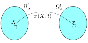
Figure 1. A schematic illustration of a flow map $\boldsymbol{x}(\boldsymbol{X},t)$ at a fixed time $t$: $\boldsymbol{x}(\boldsymbol{X},t)$ maps $\Omega_{\boldsymbol{X}}^{0}$ to $\Omega_{\boldsymbol{x}}^{t}$. $\boldsymbol{X}$ is the lagrangian coordinate while $\boldsymbol{x}$ is the Eulerian coordinate, and $F(\boldsymbol{X},t)=\frac{\partial\boldsymbol{x}(\boldsymbol{X},t)}{\partial\boldsymbol{X}}$ represents the deformation associated with the flow map.

The flow map defined by (LABEL:flow_map_AC) describes a particle moving from a initial configuration $\boldsymbol{X}$ to a instantaneous configuration $\boldsymbol{x}(\boldsymbol{X},t)$ with velocity $\boldsymbol{u}$, i.e., $\boldsymbol{x}(\boldsymbol{X},t)$ is the Eulerian coordinate and $\boldsymbol{X}$ represents Lagrangian coordinate, with the deformation tensor or Jacobian $F=\frac{\partial\boldsymbol{x}(\boldsymbol{X},t)}{\partial\boldsymbol{X}}$ [17]. which obviously satisfies $\int detFd\boldsymbol{X}=\int d\boldsymbol{x}$.

Lemma 2.1.

[15, liu2017energetic] The deformation tensor $F(\boldsymbol{x}(\boldsymbol{X},t),t)$ in Eulerian coordinate satisfies

(2.5) $$F_{t}+(\boldsymbol{u}\cdot\nabla_{\boldsymbol{x}})F=\nabla_{\boldsymbol{x}}\boldsymbol{u}F.$$

Proof.

By using the chain rule and the definition of flow map (LABEL:flow_map_AC), we obtain for $\forall i,j,k$

(2.6) $$\frac{\partial F_{ij}}{\partial t}=\frac{\partial}{\partial t}(\frac{\partial\boldsymbol{x}_{i}}{\partial\boldsymbol{X}_{j}})=\frac{\partial}{\partial\boldsymbol{X}_{j}}(\frac{\partial\boldsymbol{x}_{i}}{\partial t})=\frac{\partial}{\partial\boldsymbol{X}_{j}}\boldsymbol{u}_{i}(\boldsymbol{x}(\boldsymbol{X},t),t)=\frac{\partial\boldsymbol{u}_{i}}{\partial\boldsymbol{x}_{k}}\frac{\partial\boldsymbol{x}_{k}}{\partial\boldsymbol{X}_{j}}.$$

On the other hand, we also have

(2.7) $$\frac{\partial F(\boldsymbol{x}(\boldsymbol{X},t),t)}{\partial t}=F_{t}+(\boldsymbol{u}\cdot\nabla_{\boldsymbol{x}})F.$$

Combining (2.6) with (2.7), we obtain (2.5). ∎

Remark 2.1.

Let $f$ be the solution of the Allen-Cahn equation (2.1)-(2.2). We assume that $\boldsymbol{u}$ is the velocity such that

(2.8) $$f_{t}+(\boldsymbol{u}\cdot\nabla_{\boldsymbol{x}})f=0.$$

Then, the above transport equation and the flow map defined in (LABEL:flow_map_AC) determine the following kinematic relationship between Eulerian coordinate and Lagrangian coordinate:

(2.9) $$\frac{d}{dt}f(\boldsymbol{x}(\boldsymbol{X},t),t)=f_{t}+(\boldsymbol{u}\cdot\nabla_{\boldsymbol{x}})f=0,$$

which leads to

(2.11) $$\hat{f}_{0}(\boldsymbol{X})=f(\boldsymbol{x}(\boldsymbol{X},t),t)=f(\boldsymbol{x},0)=f_{0}(\boldsymbol{x})\quad\forall t,$$

where $\hat{f}_{0}(\boldsymbol{X})$ is the initial condition in the Lagrangian coordinate. Since $\boldsymbol{x}(\boldsymbol{X},0)=\boldsymbol{X}$, we have $\hat{f}_{0}(\cdot)=f_{0}(\cdot)$.

Once we have the flow map $\boldsymbol{x}(\boldsymbol{X},t)$, we set $\phi(\boldsymbol{X};t)=\boldsymbol{x}(\boldsymbol{X},t)$ for each $t$. Then, we derive from (2.9) that the solution of (2.1)-(2.2) is given by

(2.12) $$f(\boldsymbol{x},t)=f_{0}(\phi^{-1}(\boldsymbol{x};t)).$$

If we write $\boldsymbol{x}(\boldsymbol{X},t)=\phi(\boldsymbol{X};t)$, then from (2.9), we have $f(\boldsymbol{x},t)=f(\phi(\boldsymbol{X};t))=f_{0}(\boldsymbol{X})$. Therefore, if $f_{0}$ is such that $f_{0}(\boldsymbol{X})=f_{0}(\boldsymbol{X},0)$, then we derive from $\boldsymbol{X}=\phi^{-1}(\boldsymbol{x})$ that the function $f(\boldsymbol{x},t)$ can be determined as the composition of function

(2.13) $$f(\boldsymbol{x},t)=f_{0}\circ\phi^{-1}.$$

Once we solved $\boldsymbol{x}(\boldsymbol{X},t)=\phi(\boldsymbol{X})$, then $\phi^{-1}$ is known, and function $f$ can be solved from equation (2.13).

The central point of this new flow map approach is transforming the Eulerian coordinate into Lagrangian coordinate under which the function does not change in time, see (LABEL:essentail). Hence, if in capturing sharp interface. Since we can target all the mesh trajectories in Lagrangian coordinate and the mesh will move to the high gradient region due to the kinematic relationship we defined. If we plug the flow map (LABEL:flow_map_AC) into the transport equation (2.9), then we obtain

(2.14) $$f_{t}+\frac{d\boldsymbol{x}}{dt}\cdot\nabla_{\boldsymbol{x}}f=0.$$

It is also worthy to note that equation (2.14) can be viewed as the level set equation which is introduced by Osher and Sethian in [osher1988fronts]. It is determined by the velocity field $\boldsymbol{u}$ and the initial condition $f_{0}$ such that $\Gamma=\{\boldsymbol{x}\in R^{d}:f_{0}(\boldsymbol{x})=0\}$. The idea of level set method is transforming the Lagrangian coordinate into Eulerian coordinate by using the level set equation which is quite different with our flow dynamic approach. We try to solve the trajectory equation in Lagrangian coordinate for interface problems for our new approach.

Remark 2.2.

There is another kinematic relation $f_{t}+\nabla_{\boldsymbol{x}}\cdot(f\boldsymbol{u})=0$ describing transport of physical quantities between Eulerian coordinate and Lagrangian coordinate. Especially transport equation (2.9) can be regard as the special case of $\nabla_{\boldsymbol{x}}\cdot\boldsymbol{u}=0$. And this kinematic relation has been used to some equations that satisfy mass conservation law [carrillo2016numerical, duan2019numerical].

Assuming again the transport equation $f_{t}+\boldsymbol{u}\cdot\nabla f=0$ is satisfied, we can rewrite the Allen-Cahn equation (2.1) as

(2.15) $$\begin{split}\boldsymbol{u}\cdot\nabla_{\boldsymbol{x}}f=-\Delta_{\boldsymbol{x}}f+F^{\prime}(f).\end{split}$$

Just as the Allen-Cahn system (2.1)-(2.2), we have the new energy dissipative law for (2.15)

(2.16) $$\frac{d}{dt}\int_{\Omega_{\boldsymbol{x}}}\frac{1}{2}|\nabla_{\boldsymbol{x}}f|^{2}+F(f)d\boldsymbol{x}=-\int_{\Omega_{\boldsymbol{x}}}|\boldsymbol{u}\cdot\nabla_{\boldsymbol{x}}f|^{2}d\boldsymbol{x},$$

which is obtained by taking the inner product of the (2.15) with $f_{t}$ and using the transport equation (2.8).

The equation (2.15) can also be interpreted as a force balance relation which can be derived from the energetic variational approach. For the reader’s convenience, we provide the detail in the Appendix.

2.2. Lagrangian Formulation

Since the formulation of Allen-Cahn equation for multi-dimensions in Lagrangian coordinate are more complicated, we shall consider first the one dimension case.

Thanks to (2.11), we have the 1-D chain rule $\partial_{x}f=f^{\prime}_{0}(X)(\frac{\partial x}{\partial X})^{-1}$. Then, setting $\boldsymbol{x}=\boldsymbol{x}(\boldsymbol{X},t)$ in (2.15), we can rewrite the equation (2.15) in Lagrangian coordinate in 1-D as

(2.17) $$x_{t}(X,t)f^{\prime}_{0}(X)(\frac{\partial x}{\partial X})^{-1}=-\partial_{X}\left(f^{\prime}_{0}(X)(\frac{\partial x}{\partial X})^{-1}\right)(\frac{\partial x}{\partial X})^{-1}+F^{\prime}(f_{0}(X)),$$

(2.18) $$x|_{\partial\Omega}=X|_{\partial\Omega},~{}~{}\quad x(X,0)=X,~{}~{}X\in\Omega_{X}.$$

We observe that the last term in (2.17) is just a forcing term for the nonlinear parabolic equation in the Lagrangian coordinate. Hence, its solution $x(X,t)$ should not involve thin interfacial layers as does the solution of (2.1)-(2.2) in the Eulerian coordinate.

Remark 2.3.

The assumption that ”there exists $\boldsymbol{u}$ such that the transport equation (2.8) is satisfied” is not a unique choice, e.g., another choice is to assume

$$f_{t}+\nabla_{\boldsymbol{x}}\cdot(\boldsymbol{u}f)=0$$

which leads to an equation different from (2.15).

An assumption is suitable if the corresponding trajectory equation after the transform $\boldsymbol{x}=\boldsymbol{x}(\boldsymbol{X},t)$, i.e. (2.17)-(2.18) in the case of assumption (2.8), is well posed.

Theorem 2.1.

The system (2.17)-(2.18) satisfies the following energy dissipative law

(2.19) $$\begin{split}&\frac{d}{dt}\int_{\Omega_{X}}\frac{\partial x}{\partial X}\{\frac{1}{2}|f^{\prime}_{0}(X)(\frac{\partial x}{\partial X})^{-1}|^{2}+F(f_{0}(X))\}dX\\ &=-\int_{\Omega_{X}}\frac{\partial x}{\partial X}|x_{t}(X,t)f^{\prime}_{0}(X)(\frac{\partial x}{\partial X})^{-1}|^{2}dX.\end{split}$$

Proof.

Taking the inner product of equation (2.17) with $-x_{t}f^{\prime}_{0}(X)$, since $x_{t}|_{\partial\Omega}=0$ due to the boundary condition (2.18), we derive by integration by parts that

$$\begin{split}-\int_{\Omega_{X}}&\frac{\partial x}{\partial X}|x_{t}(X,t)f^{\prime}_{0}(X)(\frac{\partial x}{\partial X})^{-1}|^{2}dX\\ &=(\partial_{X}\left(f^{\prime}_{0}(X)(\frac{\partial x}{\partial X})^{-1}\right)(\frac{\partial x}{\partial X})^{-1},x_{t}f^{\prime}_{0}(X))-(F^{\prime}(f_{0}(X)),x_{t}f^{\prime}_{0}(X))\\ &=(\frac{1}{2}\partial_{X}|f^{\prime}_{0}(X)(\frac{\partial x}{\partial X})^{-1}|^{2},x_{t})-(\partial_{X}F(f_{0}(X)),x_{t})\\ &=-(\frac{1}{2}|f^{\prime}_{0}(X)(\frac{\partial x}{\partial X})^{-1}|^{2},\partial_{X}x_{t})+(F(f_{0}(X)),\partial_{X}x_{t})\\ &=\frac{d}{dt}\int_{\Omega_{X}}\frac{\partial x}{\partial X}\{\frac{1}{2}|f^{\prime}_{0}(X)(\frac{\partial x}{\partial X})^{-1}|^{2}+F(f_{0}(X))\}dX.\end{split}$$

The last equality is true since

$$\frac{d}{dt}\{\frac{\partial x}{\partial X}|f^{\prime}_{0}(X)(\frac{\partial x}{\partial X})^{-1}|^{2}\}=|f^{\prime}_{0}(X)|^{2}\frac{d}{dt}(\frac{\partial x}{\partial X})^{-1}=-|f^{\prime}_{0}(X)|^{2}(\frac{\partial x}{\partial X})^{-2}\frac{d}{dt}\frac{\partial x}{\partial X}.$$

∎

Remark 2.4.

We note that the energy in Eulerian coordinate

$$E(f)=\int_{\Omega_{x}}\frac{1}{2}|\partial_{x}f|^{2}+F(f)d\boldsymbol{x},$$

is equal to the energy $E(x(X,t))$ in Lagrangian coordinate,

$$E(x(X,t))=\int_{\Omega_{X}}\frac{\partial x}{\partial X}\{\frac{1}{2}|f^{\prime}_{0}(X)(\frac{\partial x}{\partial X})^{-1}|^{2}+F(f_{0}(X))\}dX.$$

This can be easily verified using the chain rule $\partial_{x}f=f^{\prime}_{0}(X)(\frac{\partial x}{\partial X})^{-1}$ and the identity $dx=\frac{\partial x}{\partial X}dX$.

Remark 2.5.

For convenience, setting $a=\frac{\partial x}{\partial X}$, suppose $a|_{t=0}>0$, then we can prove $a|_{t}>0$ for any $t>0$. We prove it by contradiction. If $a|_{t=0}>0$ and there exists a $X^{\star}$ such that $a(X^{\star},t)=0$, then we have $a_{t}<0$, $\partial_{X}a=0$ and $\partial_{X}^{2}a>0$. We rewrite equation (2.17) as

(2.20) $$\begin{split}x_{t}=-\frac{1}{f^{\prime}_{0}(X)}\partial_{X}(\frac{f^{\prime}_{0}(X)}{a})+\frac{F^{\prime}(f_{0}(X))}{f^{\prime}_{0}(X)}a\end{split}$$

If we take derivative of equation (2.20) with respect to $X$, we obtain

(2.21) $$\begin{split}a_{t}=-\frac{(ln(f^{\prime}_{0}(X)))^{\prime\prime}}{a}+\frac{f^{\prime\prime}_{0}(X)}{f^{\prime}_{0}(X)}\frac{\partial_{X}a}{a^{2}}+\frac{\partial^{2}_{X}a}{a^{2}}-\frac{2a(\partial_{X}a)^{2}}{a^{4}}+\frac{F^{\prime}(f_{0}(X))}{f^{\prime}_{0}(X)}\partial_{X}a+(\frac{F^{\prime}(f_{0}(X))}{f^{\prime}_{0}(X)})^{\prime}a.\end{split}$$

If $f^{\prime}_{0}(X)>0$, then $(ln(f^{\prime}_{0}(X)))^{\prime\prime}<0$, we derive the right hand side of equation (2.21) is larger than zero which contradicts with $a_{t}<0$.

Remark 2.6.

Since $\frac{\partial x}{\partial X}>0$ for $\forall t$, thanks to the convexity of above energy $E(x(X,t),t)$ which can be observed from (3.1) , it can be shown that the nonlinear parabolic system (2.17)-(2.18) is well posed and admits a unique solution $x(X,t)$. On the other hand, if (2.17)-(2.18) is well posed, then (2.17)-(2.18) implies (2.15). We then derive from (2.1)-(2.2) and (2.15) that the transport equation (2.8) is satisfied.

Remark 2.7.

Instead of solving (2.1)-(2.2) in the Eulerian coordinate $\boldsymbol{x}$ with potentially thin interfacial layers, such as the case if $F(f)=\frac{1}{4\epsilon^{2}}(f^{2}-1)^{2}$ with $\epsilon\ll 1$, which need to be resolved with high spatial resolution, we can solve it in the Lagrangian coordinate $\boldsymbol{X}$ free of thin interfacial layers as follows:

• Solve the flow map $\boldsymbol{x}(\boldsymbol{X},t)$ from the trajectory equation (2.17)-(2.18);

• Once we have the flow map $\boldsymbol{x}(\boldsymbol{X},t)$, the solution of (2.1)-(2.2) is given by (2.13).

3. Numerical Schemes

In this section, we construct energy stable time discretization schemes for the trajectory equation (2.17)-(2.18) in 1D.

3.1. Semi-discrete-in-time schemes

We start by constructing a first order scheme for Allen-Cahn system (2.1)-(2.2) in Lagrangian coordinate.

Given $\delta t>0$, let $t_{n}=n\delta t$, $n=0,1,2\cdots\frac{T}{\delta t}$. For any function $S(\cdot,t)$, $S^{n}$ denotes a numerical approximation to $S(\cdot,t_{n})$.

Scheme 1.

(a first order scheme)

(3.1) $$\frac{x^{n+1}-x^{n}}{\delta t}f^{\prime}_{0}(X)(\frac{\partial x^{n}}{\partial X})^{-1}=-\partial_{X}\left(f^{\prime}_{0}(X)(\frac{\partial x^{n+1}}{\partial X})^{-1}\right)(\frac{\partial x^{n+1}}{\partial X})^{-1}+F^{\prime}(f_{0}(X)),$$

(3.2) $$x^{n+1}|_{\partial\Omega}=X|_{\partial\Omega},~{}~{}\quad x^{0}(X)=X,~{}~{}X\in\Omega_{X}.$$

Remark 3.1.

Once we solve $x^{n+1}$ from (3.1)-(3.2), the approximate solution to the original equation can be obtained as $f^{n+1}(x)=f(x^{n+1}(X))=f_{0}(X)=f_{0}(\phi^{-1}(x^{n+1}))$. The above relation also indicates that the scheme (3.1)-(3.2) preserves maximum principle since $\max_{\forall n}|f(x^{n+1}(X))|=\max|f_{0}(X)|$ where $f_{0}(X)$ is the initial condition in Lagrangian coordinate.

Theorem 3.1.

Let $x^{n}$ be the solution of scheme (3.1)-(3.2) at time $t^{n}$ with $\frac{\partial x^{n}}{\partial X}>0$. Then the scheme (3.1)-(3.2) admits a unique solution $x^{n+1}$ with $\frac{\partial x^{n+1}}{\partial X}>0$, and satisfies the following discrete energy law holds:

(3.3) $$\begin{split}&\frac{E(x^{n+1})-E(x^{n})}{\delta t}\leq-\big{<}\frac{(f^{\prime}_{0}(X))^{2}}{\frac{\partial x^{n}}{\partial X}}\frac{x^{n+1}-x^{n}}{\delta t},\frac{x^{n+1}-x^{n}}{\delta t}\big{>},\end{split}$$

where $E(x)=\int_{\Omega_{X}}\{\frac{1}{2}|f^{\prime}_{0}(X)(\frac{\partial x}{\partial X})^{-1}|^{2}+F(f_{0}(X))\}\frac{\partial x}{\partial X}\,dX$.

Proof.

We first prove the existence and uniqueness of the solution of the scheme (3.1)-(3.2). To this end, we define a nonlinear functional

(3.4) $$\begin{split}J(\phi)&=\int_{\Omega_{X}}\big{\{}\frac{1}{2\delta t}\frac{(f^{\prime}_{0}(X))^{2}}{\frac{\partial x^{n}}{\partial X}}|\phi|^{2}+\frac{1}{2}(f^{\prime}_{0}(X))^{2}({\frac{\partial\phi}{\partial X}})^{-1}-g(X)\phi\big{\}}dX,\end{split}$$

with $g(X)=\frac{1}{\delta t}\frac{(f^{\prime}_{0}(X))^{2}}{\frac{\partial x^{n}}{\partial X}}+f^{\prime}_{0}(X)F(f_{0}(X))$. One can check that (3.1)-(3.2) is the Euler-Lagrange equation

$$\frac{\delta J(\phi)}{\delta\phi}|_{\phi=x^{n+1}}=0,$$

and that $J(\phi)$ is a convex functional with respect to $\phi$ with $\frac{\partial\phi}{\partial X}>0$, because of

$$\begin{split}\frac{\partial^{2}}{\partial^{2}\epsilon}\{\frac{1}{2}(f^{\prime}_{0}(X))^{2}({\frac{\partial(\phi+\epsilon\psi)}{\partial X}})^{-1}\}=(f^{\prime}_{0}(X))^{2}(\frac{\partial\phi}{\partial X})^{-3}(\frac{\partial\psi}{\partial X})^{2}\geq 0\quad\forall\psi.\end{split}$$

Hence, the scheme (3.1)-(3.2) admits a unique solution $x^{n+1}$ with $\frac{\partial x^{n+1}}{\partial X}>0$.

Next, we take the inner product of (3.1) with $-\frac{x^{n+1}-x^{n}}{\delta t}f^{\prime}_{0}(X)$ to obtain

(3.5) $$\begin{split}&\int_{\Omega_{X}}\big{\{}\partial_{X}(f^{\prime}_{0}(X)(\frac{\partial x^{n+1}}{\partial X})^{-1})(\frac{\partial x^{n+1}}{\partial X})^{-1}-F^{\prime}(f_{0}(X))\big{\}}f^{\prime}_{0}(X)\frac{x^{n+1}-x^{n}}{\delta t}dX\\ &=\int_{\Omega_{X}}\partial_{X}(f^{\prime}_{0}(X)(\frac{\partial x^{n+1}}{\partial X})^{-1})f^{\prime}_{0}(X)(\frac{\partial x^{n+1}}{\partial X})^{-1}\frac{x^{n+1}-x^{n}}{\delta t}dX\\ &-\int_{\Omega_{X}}\partial_{X}F(f_{0}(X))\frac{x^{n+1}-x^{n}}{\delta t}dX.\end{split}$$

Due to the convexity of $\frac{1}{y}$ with respect to $y$ with $y>0$, we have

$$(\frac{\partial x^{n}}{\partial X})^{-1}-(\frac{\partial x^{n+1}}{\partial X})^{-1}\geq-(\frac{\partial x^{n+1}}{\partial X})^{-2}(\frac{\partial x^{n}}{\partial X}-\frac{\partial x^{n+1}}{\partial X}),$$

which implies

(3.6) $$\begin{split}&\int_{\Omega_{X}}\partial_{X}(f^{\prime}_{0}(X)(\frac{\partial x^{n+1}}{\partial X})^{-1})f^{\prime}_{0}(X)(\frac{\partial x^{n+1}}{\partial X})^{-1}\frac{x^{n+1}-x^{n}}{\delta t}dX\\ &=-\int_{\Omega_{X}}\frac{1}{2}|f^{\prime}_{0}(X)(\frac{\partial x^{n+1}}{\partial X})^{-1}|^{2}\frac{\frac{\partial x^{n+1}}{\partial X}-\frac{\partial x^{n}}{\partial X}}{\delta t}dX\\ &\geq\frac{1}{2\delta t}\int_{\Omega_{X}}\big{(}(f^{\prime}_{0}(X))^{2}(\frac{\partial x^{n+1}}{\partial X})^{-1}-\int_{\Omega_{X}}(f^{\prime}_{0}(X))^{2}(\frac{\partial x^{n}}{\partial X})^{-1}\big{)}dX.\end{split}$$

On the other hand, we have

(3.7) $$\begin{split}-\int_{\Omega_{X}}\partial_{X}F(f_{0}(X))\frac{x^{n+1}-x^{n}}{\delta t}dX=\int_{\Omega_{X}}F(f_{0}(X))\frac{\frac{\partial x^{n+1}}{\partial X}-\frac{\partial x^{n}}{\partial X}}{\delta t}dX.\end{split}$$

We then derive (3.19) from the above two relations.

∎

Scheme 2.

(a second-order scheme)

Step 1: Compute a second-order extrapolation for $\frac{\partial x^{n+1}}{\partial X}$.

We set

(3.8) $$\frac{\partial x^{n+1}_{\star}}{\partial X}=\begin{cases}\frac{\partial(2x^{n}-x^{n-1})}{\partial X},&\text{if}\;\frac{\partial x^{n}}{\partial X}\geq\frac{\partial x^{n-1}}{\partial X},\\ \\ \frac{1}{2/{\frac{\partial x^{n}}{\partial X}}-1/{\frac{\partial x^{n-1}}{\partial X}}},&\text{if}\;\frac{\partial x^{n}}{\partial X}<\frac{\partial x^{n-1}}{\partial X}.\end{cases}$$

Step 2:

(3.9) $$\frac{3x^{n+1}-4x^{n}+x^{n-1}}{2\delta t}f^{\prime}_{0}(X)(\frac{\partial x^{n+1}_{\star}}{\partial X})^{-1}=-\partial_{X}(f^{\prime}_{0}(X)(\frac{\partial x^{n+1}}{\partial X})^{-1})(\frac{\partial x^{n+1}}{\partial X})^{-1}+F^{\prime}(f_{0}(X)),$$

(3.10) $$x^{n+1}|_{\partial\Omega}=X|_{\partial\Omega},~{}~{}\quad x^{0}(X)=X,~{}~{}X\in\Omega_{X}.$$

Theorem 3.2.

Given $x^{k}$, $k=1,2,..,n$ with $\frac{\partial x^{k}}{\partial X}>0$, the numerical scheme (3.9)-(3.10) admits a unique solution $x^{n+1}$ with $\frac{\partial x^{n+1}}{\partial X}>0$, and the following energy dissipative law is satisfied:

(3.11) $$\begin{split}\frac{E(x^{n+1})-E(x^{n})}{\delta t}\leq&-\big{<}\frac{(f^{\prime}_{0}(X))^{2}}{\frac{\partial x^{n+1}_{\star}}{\partial X}}\frac{x^{n+1}-x^{n}}{\delta t},\frac{x^{n+1}-x^{n}}{\delta t}\big{>}\\ &-\big{<}\frac{(f^{\prime}_{0}(X))^{2}}{\frac{\partial x^{n+1}_{\star}}{\partial X}}\frac{x^{n+1}-2x^{n}+x^{n-1}}{2\delta t},\frac{x^{n+1}-2x^{n}+x^{n-1}}{2\delta t}\big{>},\end{split}$$

where

(3.12) $$\begin{split}E(x^{n+1})&=\int_{\Omega_{X}}\frac{\partial x^{n+1}}{\partial X}\{\frac{1}{2}|f^{\prime}_{0}(X)(\frac{\partial x^{n+1}}{\partial X})^{-1}|^{2}+F(f_{0}(X))\}dX\\ &+\frac{1}{4\delta t}\int_{\Omega_{X}}(f^{\prime}_{0}(X))^{2}(\frac{\partial x^{n+1}_{\star}}{\partial X})^{-1}|x^{n+1}-x^{n}|^{2}dX.\end{split}$$

Proof.

As in the proof of Theorem 3.1, one can construct a convex functional such that its Euler Lagrange equation is equivalent to the scheme (3.9)-(3.10). Hence, the scheme admits a unique solution $x^{n+1}$ with $\frac{\partial x^{n+1}}{\partial X}>0$.

Next, taking the inner product of equation (3.9) with $-f_{0}^{\prime}(X)\frac{x^{n+1}-x^{n}}{\delta t}$ and using the equality,

(3.13) $$(3a-4b+c,2(a-b))=5|a-b|^{2}-|b-c|^{2}+|a-2b+c|,$$

the left hand side becomes

(3.14) $$\begin{split}-(\frac{3x^{n+1}-4x^{n}+x^{n-1}}{2\delta t}&(f^{\prime}_{0}(X))^{2}(\frac{\partial x^{n+1}_{\star}}{\partial X})^{-1},\frac{x^{n+1}-x^{n}}{\delta t})\\ =&-5\int_{\Omega_{X}}\frac{1}{4\delta t^{2}}(f^{\prime}_{0}(X))^{2}(\frac{\partial x^{n+1}_{\star}}{\partial X})^{-1}|x^{n+1}-x^{n}|^{2}dX\\ &+\int_{\Omega_{X}}\frac{1}{4\delta t^{2}}(f^{\prime}_{0}(X))^{2}(\frac{\partial x^{n+1}_{\star}}{\partial X})^{-1}|x^{n}-x^{n-1}|^{2}dX\\ &-\int_{\Omega_{X}}\frac{1}{4\delta t^{2}}(f^{\prime}_{0}(X))^{2}(\frac{\partial x^{n+1}_{\star}}{\partial X})^{-1}|x^{n+1}-2x^{n}+x^{n-1}|^{2}dX.\end{split}$$

The right hand side can be treated exactly the same way as in the proof of Theorem 3.1, see (3.5)-(3.6). Combining these results, we derive the following energy dissipative law

$$\begin{split}\frac{E(x^{n+1})-E(x^{n})}{\delta t}&\leq-\frac{1}{\delta t^{2}}\int_{\Omega_{X}}(f^{\prime}_{0}(X))^{2}(\frac{\partial x^{n+1}_{\star}}{\partial X})^{-1}|x^{n+1}-x^{n}|^{2}dX\\ &-\frac{1}{4\delta t^{2}}\int_{\Omega_{X}}(f^{\prime}_{0}(X))^{2}(\frac{\partial x^{n+1}_{\star}}{\partial X})^{-1}|x^{n+1}-2x^{n}+x^{n-1}|^{2}dX.\end{split}$$

∎

Remark 3.2.

If we consider logarithmic free energy function $F(f)=\frac{\theta}{2}[(1+f)\log(1+f)+(1-u)\log(1-u)]-\frac{\theta_{c}}{2}f^{2}$, where $\theta,\theta_{c}$ are two positive constants. Since $F^{\prime}(f_{0}(X))$ is known in Scheme 1 and Scheme 2, so the positive property of solution $0<1-f^{n+1},0<f^{n+1}+1$ is preserved naturally. Then comparing with numerical methods in Eulerian coordinate, it is more convenient to solve Allen-Cahn equation with logarithmic free energy by using flow dynamic approach.

3.2. Fully discrete schemes

We now describe fully discrete schemes with a Galerkin approximation in space. For the sake of brevity, we only consider fully discretization for Scheme 1. Fully discretization for Scheme 2 can be constructed similarly.

Let $V_{h}\in H^{1}(\Omega_{X})$ be a finite dimensional approximation space and $V^{0}_{h}=V_{h}\cup H^{1}_{0}(\Omega_{X})$, a fully discrete version of Scheme 1 is: Find $x_{h}^{n+1}\in V_{h}$ such that

$$(\frac{1}{2}|f_{0}^{\prime}(X)(\frac{\partial x_{h}^{n+1}}{\partial X})^{-1}|^{2},\partial_{X}y_{h})+(F^{\prime}(f_{0}(X)),y_{h}f^{\prime}_{0}(X))$$

(3.15) $$\hskip 72.26999pt=(\frac{x_{h}^{n+1}-x_{h}^{n}}{\delta t}f^{\prime}_{0}(X)(\frac{\partial x_{h}^{n}}{\partial X})^{-1},y_{h}f^{\prime}_{0}(X)),\quad\forall y_{h}\in V_{h}^{0},$$

(3.16) $$x_{h}^{n+1}|_{\partial\Omega}=X|_{\partial\Omega},\quad x_{h}^{0}(X)=X,~{}~{}X\in\Omega.$$

In our numerical tests, we set the domain to be $\Omega_{x}=\Omega_{X}=(-1,1)$, and use two different spatial discretizations. The first is the Legendre-Galerkin method [30] with

(3.17) $$V_{h}:=V_{N}=\text{span}\{L_{j}(x):j=0,1,\cdots,N\},$$

where $L_{j}(x)$ is the Legendre polynomial of $j-$th degree, and

(3.18) $$V^{0}_{h}:=V^{0}_{N}=\text{span}\{\phi_{j}(x):=L_{j}(x)-L_{j+2}(x):j=0,1,\cdots,N-2\}.$$

The other is the piecewise linear finite-element method.

The scheme (3.15)-(3.16) leads to a nonlinear system: $G(x_{h}^{n+1})=0$ at each time step, which can be effectively solved by using, for example, a damped Newton’s iteration [27]:

$$x_{h}^{n+1,k+1}=x^{n+1,k}_{h}-\alpha(\delta_{x})(\nabla G(x^{n+1,k}_{h}))^{-1}G(x^{n+1,k}_{h}),$$

with $\alpha=O(\epsilon^{2})$ as the damped coefficient.

Using exactly the same arguments as in the proof of Theorem 3.1, we can establish the following:

Theorem 3.3.

Given $x_{h}^{n}\in V_{h}$ with $\frac{\partial x_{h}^{n}}{\partial X}>0$. Then the scheme (3.15)-(3.16) admits a unique solution $x_{h}^{n+1}$ with $\frac{\partial x_{h}^{n+1}}{\partial X}>0$, and satisfies the following discrete energy law holds:

(3.19) $$\begin{split}&\frac{E(x_{h}^{n+1})-E(x_{h}^{n})}{\delta t}\leq-\big{<}\frac{(f^{\prime}_{0}(X))^{2}}{\frac{\partial x_{h}^{n}}{\partial X}}\frac{x_{h}^{n+1}-x_{h}^{n}}{\delta t},\frac{x_{h}^{n+1}-x_{h}^{n}}{\delta t}\big{>},\end{split}$$

where $E(x)=\int_{\Omega_{X}}\{\frac{1}{2}|f^{\prime}_{0}(X)(\frac{\partial x}{\partial X})^{-1}|^{2}+F(f_{0}(X))\}\frac{\partial x}{\partial X}\,dX$.

3.3. Hybird coordinate method

We would like to mention that how to choose $f_{0}$ in (LABEL:comp:N) or (LABEL:comp:h) is very important. Formally we set $f_{0}$ as the initial condition, but if the initial condition can not provide enough information. This motivate us to obtain $f_{0}$ from Eulerian coordinate. So we improve a hybird coordinate method below.

Scheme 3.

(Hybird Coordinate Scheme) For simplicity we introduce a first order scheme for the generalized Allen-Cahn equation in hybird coordinate. In Eulerian coordinate we can choose full implicit or any convex splitting method in time and in Lagrangian coordinate we can use the numerical methods we proposed above.

Step 1:  Compute $f_{0}(X)$ in Eulerian coordinate

$$\begin{split}&\frac{f_{N}^{n+1}-f_{N}^{n}}{\delta t}-\partial_{xx}f_{N}^{n+1}+\frac{1}{\epsilon^{2}}f_{N}^{n+1}((f_{N}^{n+1})^{2}-1)=0,\\ &f(x,0)=f_{0}(x),\quad f_{N}(x,t)|_{\partial\Omega}=f(x,0)|_{\partial\Omega}.\end{split}$$

Once $f_{N}^{n+1}(x)$ is solved in Eulerian coordinate then we define $f_{0}(X)=f^{n+1}(x)$ for (2.13) and initial condition as $x(X,0)=X$ in Lagrangian coordinate below,

Step 2:   Compute $x_{N}^{n+1}$ in Lagrangian coordinate

$$\begin{split}&\frac{x_{N}^{n+1}-x_{N}^{n}}{\delta t}f^{\prime}_{0}(X)(\frac{\partial x_{N}^{n}}{\partial X})^{-1}-\partial_{X}(f^{\prime}_{0}(X)(\frac{\partial x_{N}^{n+1}}{\partial X})^{-1})(\frac{\partial x_{N}^{n+1}}{\partial X})^{-1}+F^{\prime}(f_{0}(X))=0,\\ &x_{N}^{n+1}|_{\partial\Omega}=X|_{\partial\Omega},\quad x^{0}(X)=X,~{}~{}X\in\Omega_{X}.\end{split}$$

Step 3:  Compute $f_{N}^{n+1}(x)$ by composition (LABEL:comp:N) .

Remark 3.3.

Hybird Coordinate Scheme will also enjoy good properties like preserving energy dissipative law or maximum principle, if numerical methods we used in Eulerian coordinate and Lagrangian coordinate provide such good properties.

4. Some extensions

We consider in the section two immediate extensions of our flow dynamic approach.

4.1. Allen-Cahn equation with advection

We consider here a generalized Allen-cahn equation (4.1) with an advection term:

(4.1) $$f_{t}+{\mathbf{v}}\cdot\nabla_{\boldsymbol{x}}f=(\Delta_{\boldsymbol{x}}f-\frac{1}{\epsilon^{2}}f(f^{2}-1)),$$

where ${\mathbf{v}}$ is a given velocity field. We still assume that there exists a velocity field $\boldsymbol{u}$ satisfying the kinematic equation

(4.2) $$f_{t}+\boldsymbol{u}\cdot\nabla_{\boldsymbol{x}}f=0,$$

so we can define the flow map (LABEL:flow_map_AC). Using (4.2), we can rewrite (4.1) as

(4.3) $$({\mathbf{v}}-\boldsymbol{u})\cdot\nabla_{\boldsymbol{x}}f=\Delta_{\boldsymbol{x}}f-\frac{1}{\epsilon^{2}}f(f^{2}-1).$$

Note that the above force balance equation can also be derived using the energetic variational formulation using the Least action principle and Maximum dissipative law (see the Appendix). Taking the inner product of the above equation with $f_{t}$, thanks to (4.2), we can derive the following energy dissipation law:

(4.4) $$\frac{d}{dt}\int_{\Omega_{\boldsymbol{x}}}\frac{1}{2}|\nabla_{\boldsymbol{x}}f|^{2}+\frac{1}{4\epsilon^{2}}(f^{2}-1)^{2}d\boldsymbol{x}=-\int_{\Omega_{\boldsymbol{x}}}|({\mathbf{v}}-\boldsymbol{u})\cdot\nabla_{\boldsymbol{x}}f|^{2}d\boldsymbol{x}.$$

Let us consider now the 1-D case. By using the flow map $\frac{dx(X,t)}{dt}=\boldsymbol{u}$ and the chain rule $\partial_{x}f=f^{\prime}_{0}(X)(\frac{\partial x}{\partial X})^{-1}$, we can derive from (4.3) in Eulerian coordinate the trajectory equation in Lagrangian coordinate:

(4.5) $$(x_{t}(X,t)-{\mathbf{v}})f^{\prime}_{0}(X)(\frac{\partial x}{\partial X})^{-1}=-\partial_{X}(f^{\prime}_{0}(X)(\frac{\partial x}{\partial X})^{-1})(\frac{\partial x}{\partial X})^{-1}+F^{\prime}(f_{0}(X)),$$

(4.6) $$x|_{\partial\Omega}=X|_{\partial\Omega}~{}~{}\mbox{and}~{}~{}\quad x(X,0)=X,~{}~{}X\in\Omega.$$

Similar to the trajectory equation (2.17) for the Allen-Cahn equation, we can construct first- and second-order schemes for (4.6) as in the last section. We leave the detail to the interested readers.

4.2. Two dimensional axis-symmetric case

We consider the Allen-Cahn equation (2.2) in a two dimensional axis-symmetric domain $\Omega$. To fix the idea, we set $\Omega=\{x^{2}+y^{2}<h^{2}\}$. Using the polar transform $x=rcos(\theta),y=rsin(\theta)$, we can rewrite (2.2) in polar coordinates for the axis-symmetric case as

(4.7) $$\begin{split}&f_{t}-\frac{1}{r}\partial_{r}(r\partial_{r}f)+F^{\prime}(f)=0;\quad f(h,t)=0\\ &f(r,0)=f_{0}(r),\end{split}$$

and the associated flow map (LABEL:flow_map_AC) for the axis-symmetric case as

(4.8) $$\begin{split}&\frac{dr(R,t)}{dt}=u,\\ &r(R,0)=R,\end{split}$$

where $R$ is the Lagrangian coordinate and $r$ is Eulerian coordinate. Then, the assumed transport equation (2.8) takes the form

(4.10) $$f_{t}+uf_{r}=f_{t}+\frac{dr(R,t)}{dt}f_{r}=0,$$

$$f|_{t=0}=f_{0}(r),$$

which is equivalent to $f(r(R,t),t)=f(r,0)=f_{0}(R)$ because of flow map (4.8) (cf. Remark 2.1). We then derive from (4.10) and (4.7) the following force balance equation

(4.11) $$\frac{dr(R,t)}{dt}f_{r}=-\frac{1}{r}\partial_{r}(r\partial_{r}f)+F^{\prime}(f).$$

Using the chain rule $\partial_{r}f=f_{0}^{\prime}(R)(\frac{\partial r}{\partial R})^{-1}$, we arrive at the trajectory equation in polar coordinate:

(4.12) $$\begin{split}&r_{t}(\frac{\partial r}{\partial R})^{-1}\partial_{R}f_{0}(R)=-\frac{1}{r(R)}(\frac{\partial r}{\partial R})^{-1}\partial_{R}(r(R)(\frac{\partial r}{\partial R})^{-1}\partial_{R}f_{0}(R))+F^{\prime}(f_{0}(R)),\\ &r(h,t)=h,\;r(R,0)=R.\end{split}$$

Theorem 4.1.

The Allen-Cahn equation in Lagrangian coordiante (4.12) satisfies the following energy dissipative law

(4.13) $$\begin{split}&\frac{d}{dt}\int_{\Omega_{R}}\{\frac{1}{2}|(\frac{\partial r}{\partial R})^{-1}\partial_{R}f_{0}(R)|^{2}+F(f_{0}(R))\}det\frac{\partial r}{\partial R}RdR\\ &=-\int_{\Omega_{R}}|r_{t}\partial_{R}f_{0}(R))(\frac{\partial r}{\partial R})^{-1}|^{2}det\frac{\partial r}{\partial R}RdR.\end{split}$$

Proof.

Taking inner product of equation (4.12) with $-rr_{t}\partial_{R}f_{0}(R)$, we obtain

(4.14) $$\begin{split}&(r_{t}(\frac{\partial r}{\partial R})^{-1}\partial_{R}f_{0}(R),-rr_{t}\partial_{R}f_{0}(R))=(-\frac{1}{r(R)}(\frac{\partial r}{\partial R})^{-1}\partial_{R}(r(R)(\frac{\partial r}{\partial R})^{-1}\partial_{R}f_{0}(R)),-rr_{t}\partial_{R}f_{0}(R))\\ &\hskip 113.81102pt+(F^{\prime}(f_{0}(R)),-rr_{t}\partial_{R}f_{0}(R)).\end{split}$$

Notice that $\int_{\Omega_{r}}rdr=\int_{\Omega_{R}}det\frac{\partial r}{\partial R}RdR=\int_{\Omega_{R}}rr^{\prime}(R)dR$, we derive the equality

(4.15) $$det\frac{\partial r}{\partial R}=\frac{r\frac{\partial r}{\partial R}}{R}.$$

We obtain

(4.16) $$\begin{split}&(r_{t}(\frac{\partial r}{\partial R})^{-1}\partial_{R}f_{0}(R),-rr_{t}\partial_{R}f_{0}(R))=-\int_{\Omega_{R}}|r_{t}\partial_{R}f_{0}(R))(\frac{\partial r}{\partial R})^{-1}|^{2}r\frac{\partial r}{\partial R}dR\\ &=-\int_{\Omega_{R}}|r_{t}\partial_{R}f_{0}(R))(\frac{\partial r}{\partial R})^{-1}|^{2}det\frac{\partial r}{\partial R}RdR.\end{split}$$

Taking integration by part, we derive

(4.17) $$\begin{split}&(F^{\prime}(f_{0}(R)),-rr_{t}\partial_{R}f_{0}(R))=(\partial_{R}F(f_{0}(R)),-rr_{t})=(F(f_{0}(R)),\frac{\partial r}{\partial R}r_{t}+r\frac{\partial r_{t}}{\partial R})\\ &=\frac{d}{dt}\int_{\Omega_{R}}F(f_{0}(R))r\frac{\partial r}{\partial R}dR=\frac{d}{dt}\int_{\Omega_{R}}F(f_{0}(R))det\frac{\partial r}{\partial R}RdR.\end{split}$$

We consider

(4.18) $$\begin{split}&(-\frac{1}{r(R)}(\frac{\partial r}{\partial R})^{-1}\partial_{R}(r(R)(\frac{\partial r}{\partial R})^{-1}\partial_{R}f_{0}(R)),-rr_{t}\partial_{R}f_{0}(R))=(\frac{1}{2}\partial_{R}|r(R)(\frac{\partial r}{\partial R})^{-1}\partial_{R}f_{0}(R)|^{2},\frac{r_{t}}{r})\\ &=-(\frac{1}{2}|r(\frac{\partial r}{\partial R})^{-1}\partial_{R}f_{0}(R)|^{2},\partial_{R}(\frac{r_{t}}{r}))=-(\frac{1}{2}|(\frac{\partial r}{\partial R})^{-1}\partial_{R}f_{0}(R)|^{2},rr_{tR}-r_{t}\frac{\partial r}{\partial R})\\ &=\frac{d}{dt}\int_{\Omega_{R}}\frac{1}{2}|\partial_{R}f_{0}(R)|^{2}r(\frac{\partial r}{\partial R})^{-1}dR=\frac{d}{dt}\int_{\Omega_{R}}\frac{1}{2}|(\frac{\partial r}{\partial R})^{-1}\partial_{R}f_{0}(R)|^{2}r\frac{\partial r}{\partial R}dR\\ &=\frac{d}{dt}\int_{\Omega_{R}}\frac{1}{2}|(\frac{\partial r}{\partial R})^{-1}\partial_{R}f_{0}(R)|^{2}det\frac{\partial r}{\partial R}RdR.\end{split}$$

Finally, combining equations (4.16)-(4.18), we obtain the energy dissipative law.

∎

Remark 4.1.

Similar with Remark 2.4, the energy dissipative law in Theorem 4.1 is equivalent with energy dissipative law in Eulerian coordinate by using the chain rule $\partial_{r}f=f_{0}^{\prime}(R)(\frac{\partial r}{\partial R})^{-1}$,

(4.19) $$\frac{d}{dt}\int_{\Omega_{r}}\{\frac{1}{2}|\partial_{r}f|^{2}+\frac{1}{4\epsilon^{2}}(f^{2}-1)^{2}\}rdr=-\int_{\Omega_{r}}|uf_{r}|^{2}rdr.$$

Similarly, we can construct first and second schemes for the above equation. For example, a first-order scheme for (4.12) is as follows:

(4.20) $$\begin{split}&\frac{r^{n+1}-r^{n}}{\delta t}(\frac{\partial r^{n}}{\partial R})^{-1}\partial_{R}f_{0}(R)=-(\frac{\partial r^{n+1}}{\partial R})^{-1}\partial_{R}((\frac{\partial r^{n+1}}{\partial R})^{-1}\partial_{R}f_{0}(R))\\ &-\frac{1}{r^{n+1}(R)}(\frac{\partial r^{n+1}}{\partial R})^{-1}\partial_{R}f_{0}(R)+F^{\prime}(f_{0}(R)),\\ &r^{n+1}|_{r=h}=h,\,r(R,0)=R.\end{split}$$

5. Numerical experiments

In this section, we present some numerical tests to show the efficiency, stability and accuracy of the numerical schemes (3.15)-(3.16) and its second-order version for the Allen-Cahn equation (2.1)-(2.2) with $F(f)=\frac{1}{4\epsilon^{2}}(f^{2}-1)^{2}$. In the following, we set $\Omega_{x}=\Omega_{X}=(-1,1)$ and use, as spatial discretization, the Legendre-Galerkin method [30] and the piecewise linear finite-element method.

We set the domain to be $\Omega_{x}=\Omega_{X}=(-1,1)$, and use two different spatial discretizations in our numerical tests. The first is the Legendre-Galerkin method [30] with

(5.1) $$V_{h}:=V_{N}=\text{span}\{L_{j}(x):j=0,1,\cdots,N\},$$

where $L_{j}(x)$ is the Legendre polynomial of $j-$th degree, and

(5.2) $$V^{0}_{h}:=V^{0}_{N}=\text{span}\{\phi_{j}(x):=L_{j}(x)-L_{j+2}(x):j=0,1,\cdots,N-2\}.$$

The other one is the piecewise linear finite-element method.

The scheme (3.15)-(3.16) leads to a nonlinear system: $G(x_{h}^{n+1})=0$ at each time step. The standard Newton’s iteration may not work well when $\epsilon\ll 1$, so we use a damped Newton’s iteration [27]:

$$x_{h}^{n+1,k+1}=x^{n+1,k}_{h}-\alpha(\delta_{x})(\nabla G(x^{n+1,k}_{h}))^{-1}G(x^{n+1,k}_{h}),$$

with $\alpha=O(\epsilon^{2})$ as the damped coefficient.

Remark 5.1.

If the initial condition $f_{0}(x)$ in the Eulerian coordinate is ”smooth”, one can use a coarse mesh independent of $\epsilon$ in (3.15)-(3.16).

However, if $f_{0}(x)$ is a randomized initial condition or already with thin interfacial layers, we need to start with a $\epsilon$ dependent mesh, which is fine enough to resolve the thin interfacial layers, compute a sufficient time steps such that the solution becomes smooth, then switch to a coarse mesh independent of $\epsilon$.

5.1. Accuracy test

We first perform an accuracy test. We used Legendre-Galerkin method in space so that the spatial error is negligible compared with the temporal error. We start with a smooth initial condition $f_{0}(x)=x$ and using solution computed by the second-order scheme with $\delta t=10^{-5}$ as the reference solution. In Fig. 2 we plot the $L^{\infty}$ error between numerical solution and reference solution at time $t=0.1$. We observe that the first-order scheme BDF1 achieves first-order convergence while the second-order scheme BDF2 achieves second-order convergence.

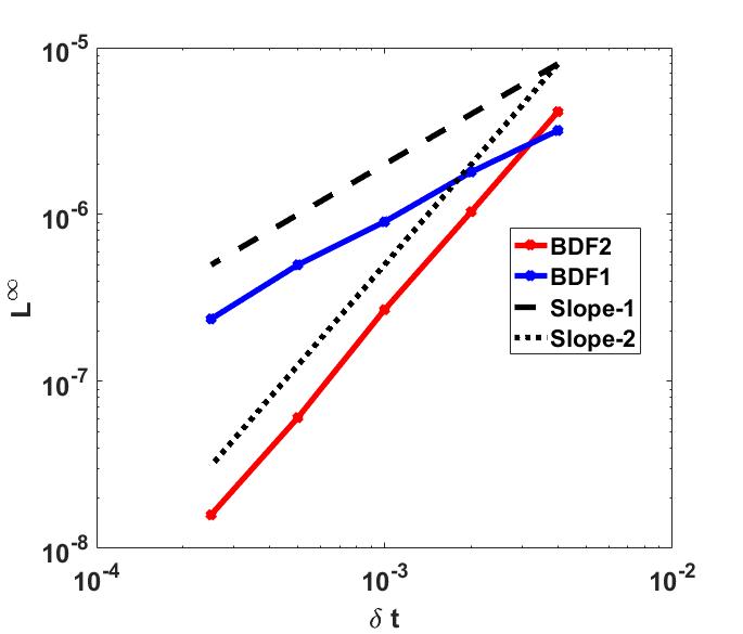
Figure 2. Accuracy test for the Allen-Cahn equation (2.1)-(2.2).

5.2. Interface capturing

We now present numerical simulations to demonstrate the effectiveness of our new Lagrangian approach for interface capturing. In Fig. 3 we choose interface width parameter as $\epsilon^{2}=0.001$ and initial condition as $f_{0}(x)=1-x^{2}$. We depict profiles of interface at various time in Fig. 3.(a) and in Fig. 3.(b) using the second-order new Lagrangian scheme with spectral method and finite element method in space, and in Fig. 3.(c) using the second-order semi-implicit method in Eulerian coordinate with spectral method in space. We observe that the profiles of interface can be well captured with mesh resolution of $N=64$ by the Lagrangian method, as compared with $N=256$ by the Eulerian method. We also plot in Fig. 3.(d), the mesh distribution of the Lagrangian method in Eulerian coordinate. We observe that as interface getting steeper, more points will move closer to the interface area.

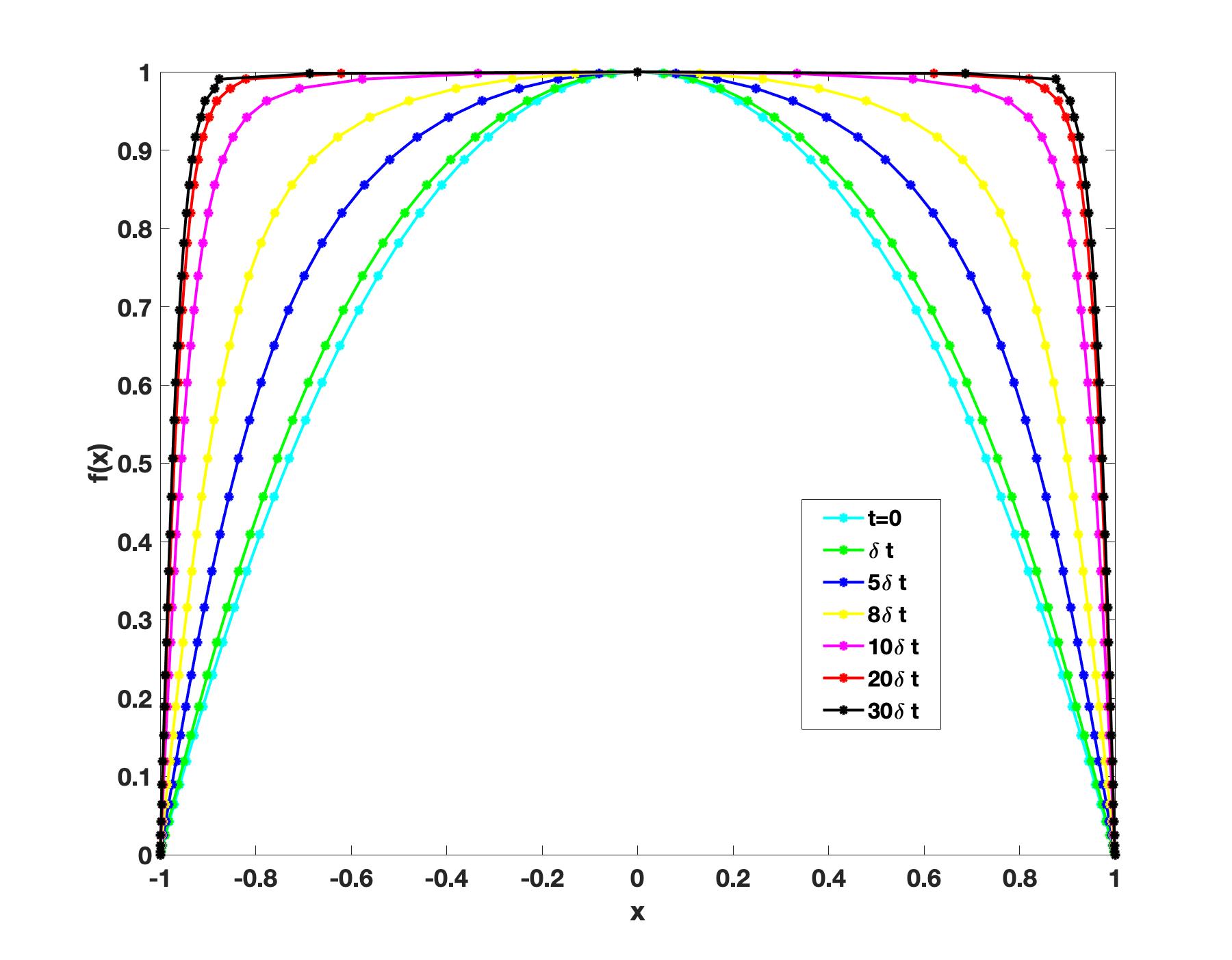
(a) Flow dynamic approach with Spectral method:$N=64$ and $\epsilon^{2}=0.001$.

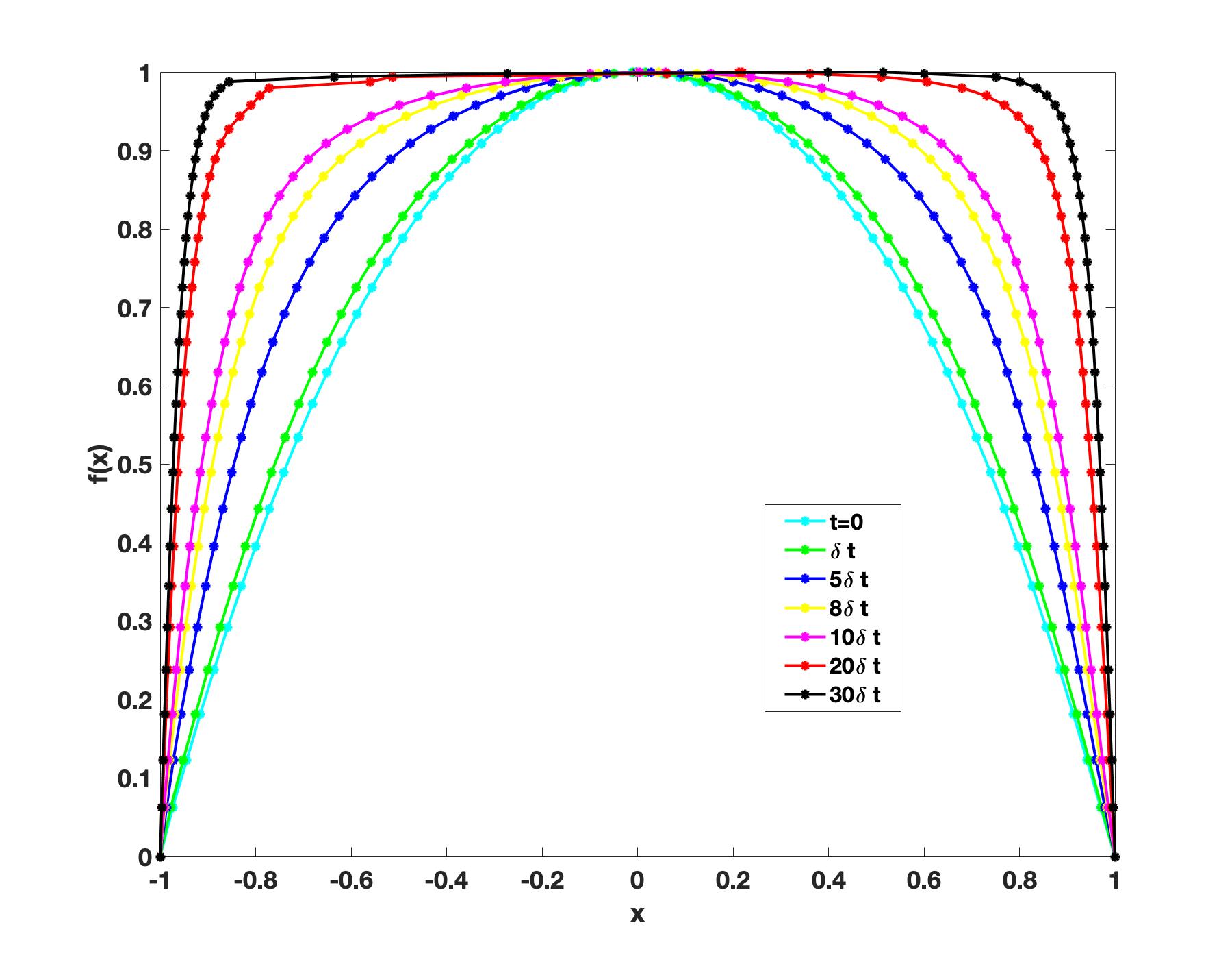
(b) Flow dynamic approach with Finite element method: $N=64$ and $\epsilon^{2}=0.001$.

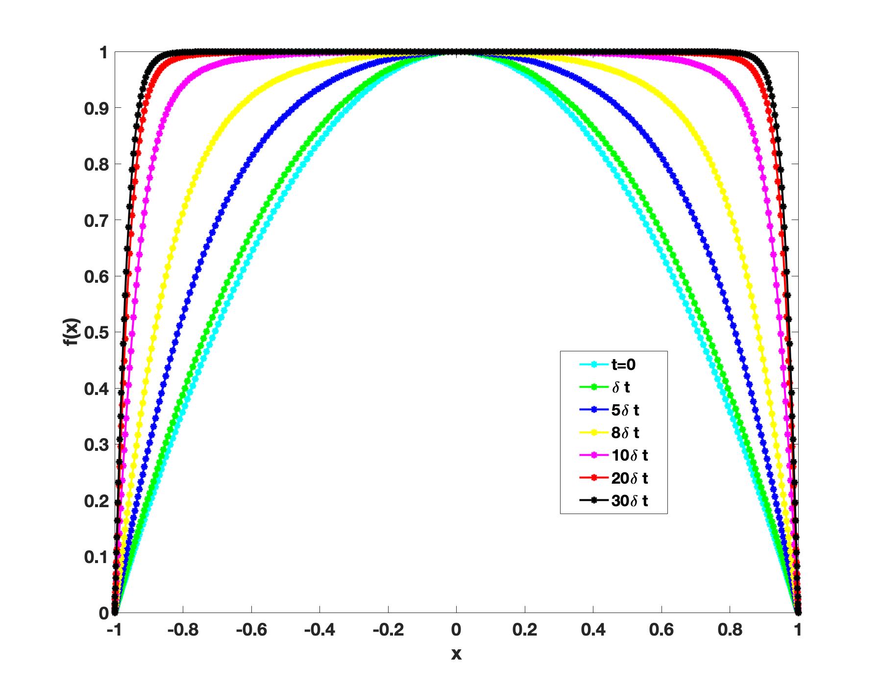
(c) Numerical method in Eulerian coordinate $N=256$ and $\epsilon^{2}=0.001$.

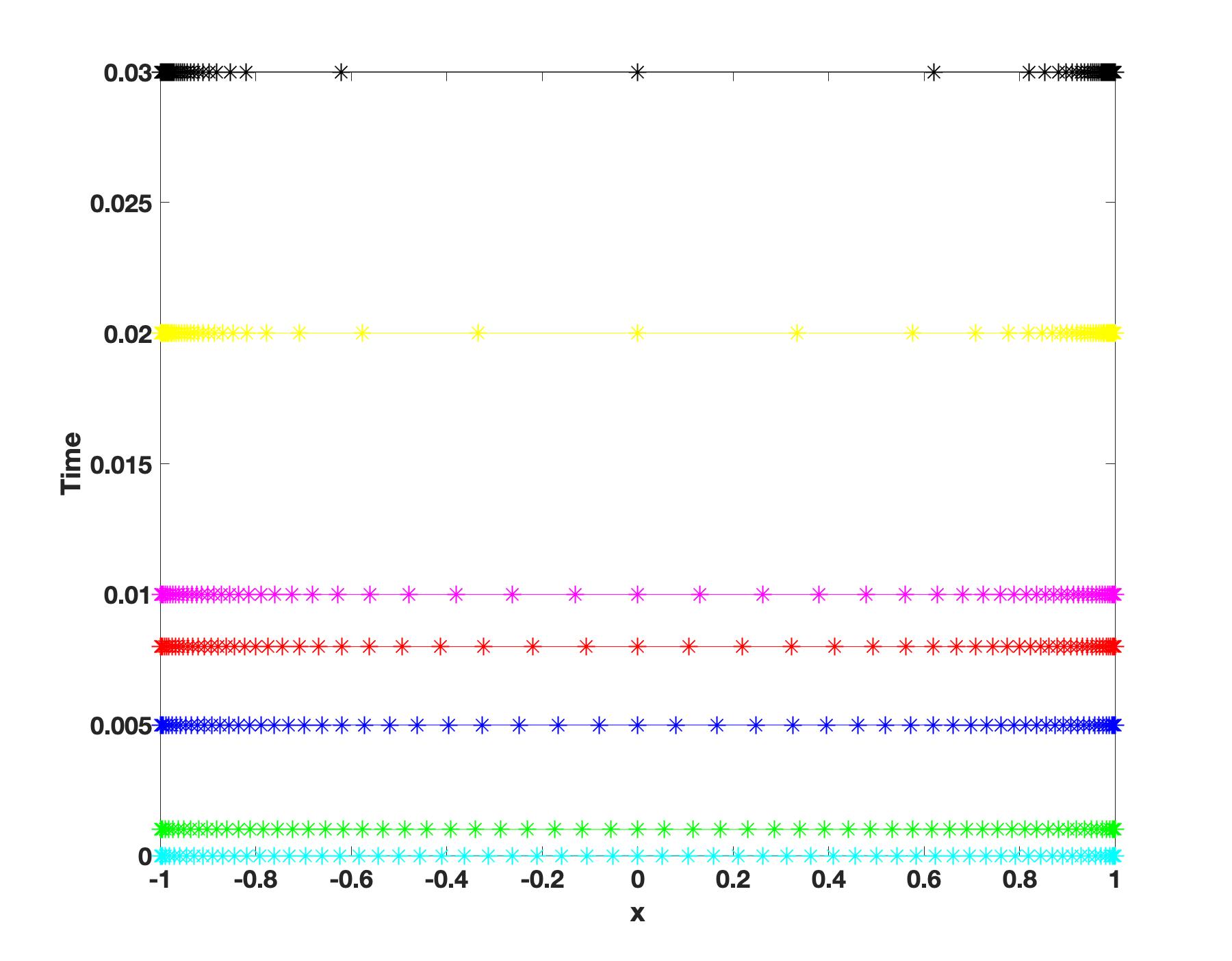
(d) Mesh distribution for Flow dynamic approach.

Figure 3. Capturing interface by Lagrangian numerical method based on Variational Energetic Approach.

Next we examine what happens as we decrease the interfacial width. It is expected that the solution, in the limit of $\epsilon$ going to zero, behaves like a piecewise constant function with values $\pm 1$ in much of two bulk regions which are separated by a diffusive interfacial layer of thickness $O(\epsilon)$.

We first use the Lagrangian scheme with the finite-element method in space. In Fig. 4, we plot the results for $\epsilon^{2}=10^{-3}$ to $\epsilon^{2}=10^{-6}$ with $N=8,16,32,64$ points and initial condition is $f_{0}(x)=x$. We observe that almost all points are concentrated at the interfacial region. The interface location is well captured even with only 8 points, although the value is a bit off due to the limited accuracy of finite-elements. We obtain similar results as we decrease $\epsilon$ further. This example shows the amazing ability of the flow dynamic approach in capturing thin interfaces of Allen-Cahn equations: the number of points needed to resolve the interface is independent of interfacial width!

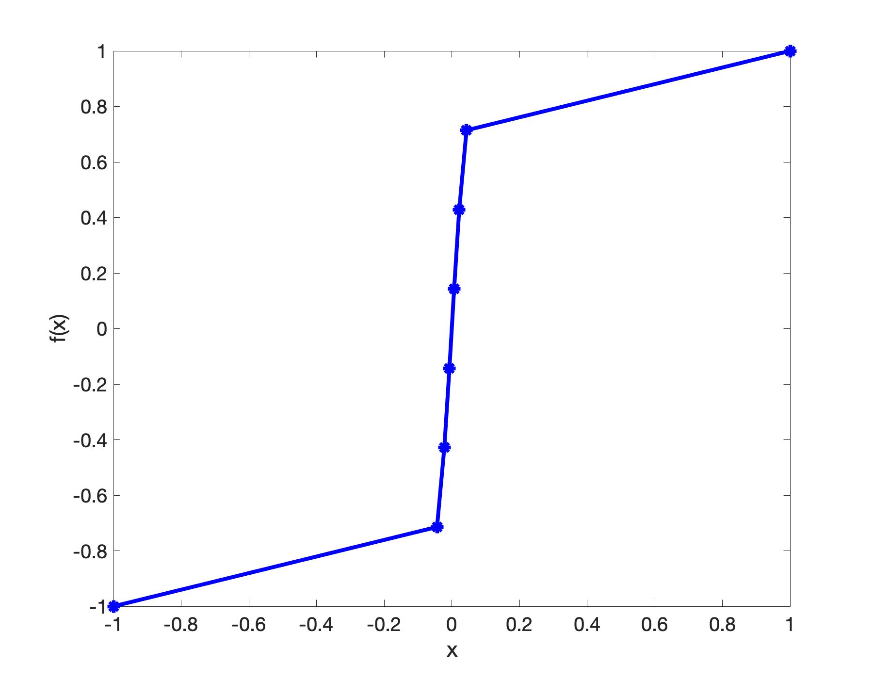
(a) $\epsilon^{2}=10^{-3}$ and $N=8$.

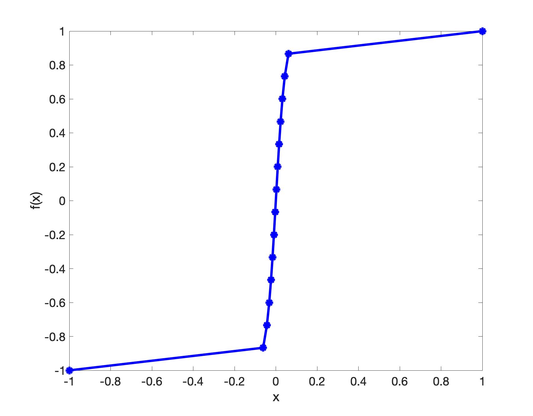
(b) $\epsilon^{2}=10^{-3}$ and $N=16$ .

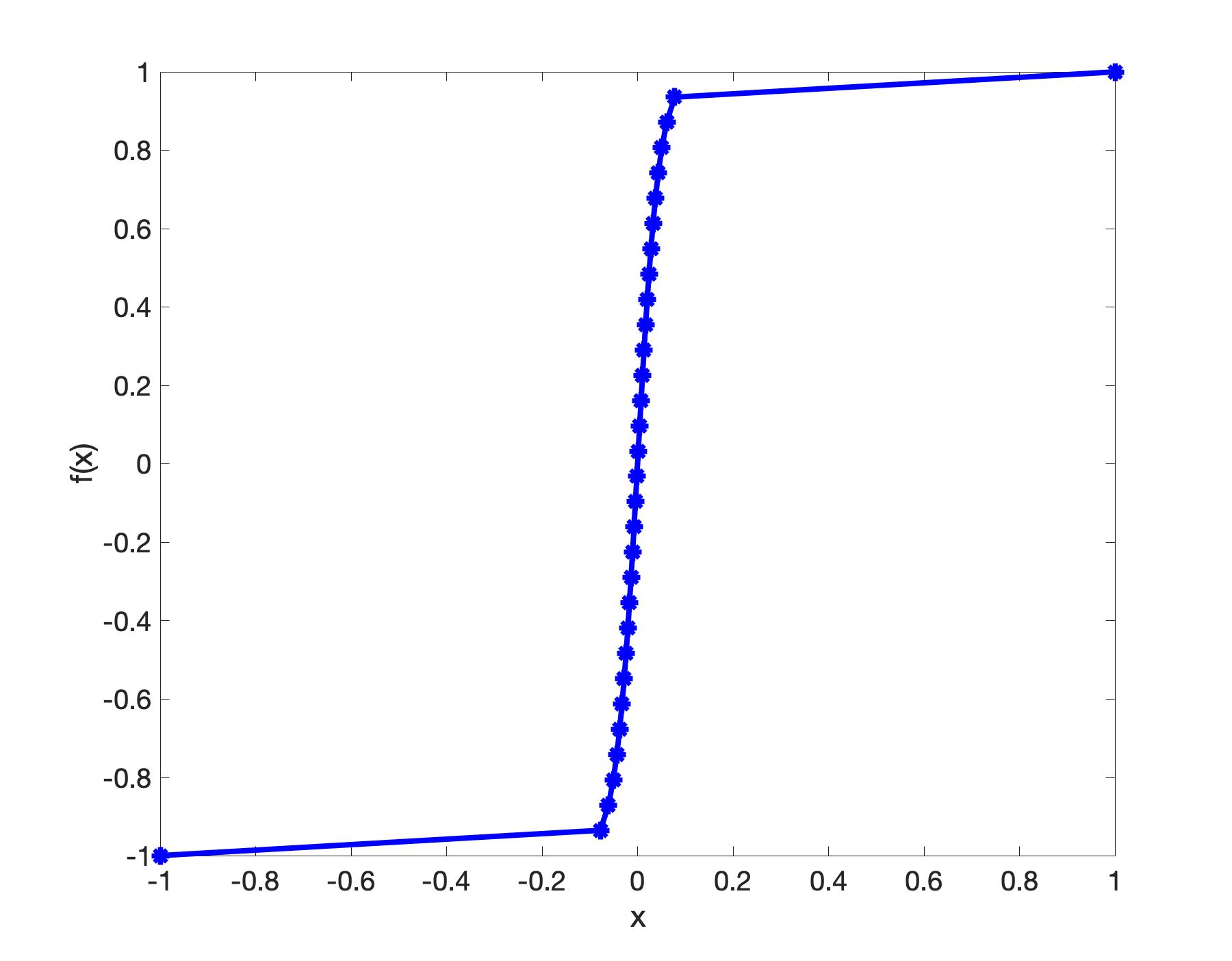
(c) $\epsilon^{2}=10^{-3}$ and $N=32$

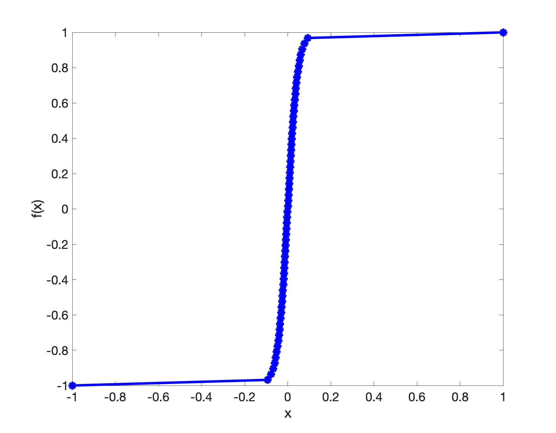
(d) $\epsilon^{2}=10^{-3}$ and $N=64$

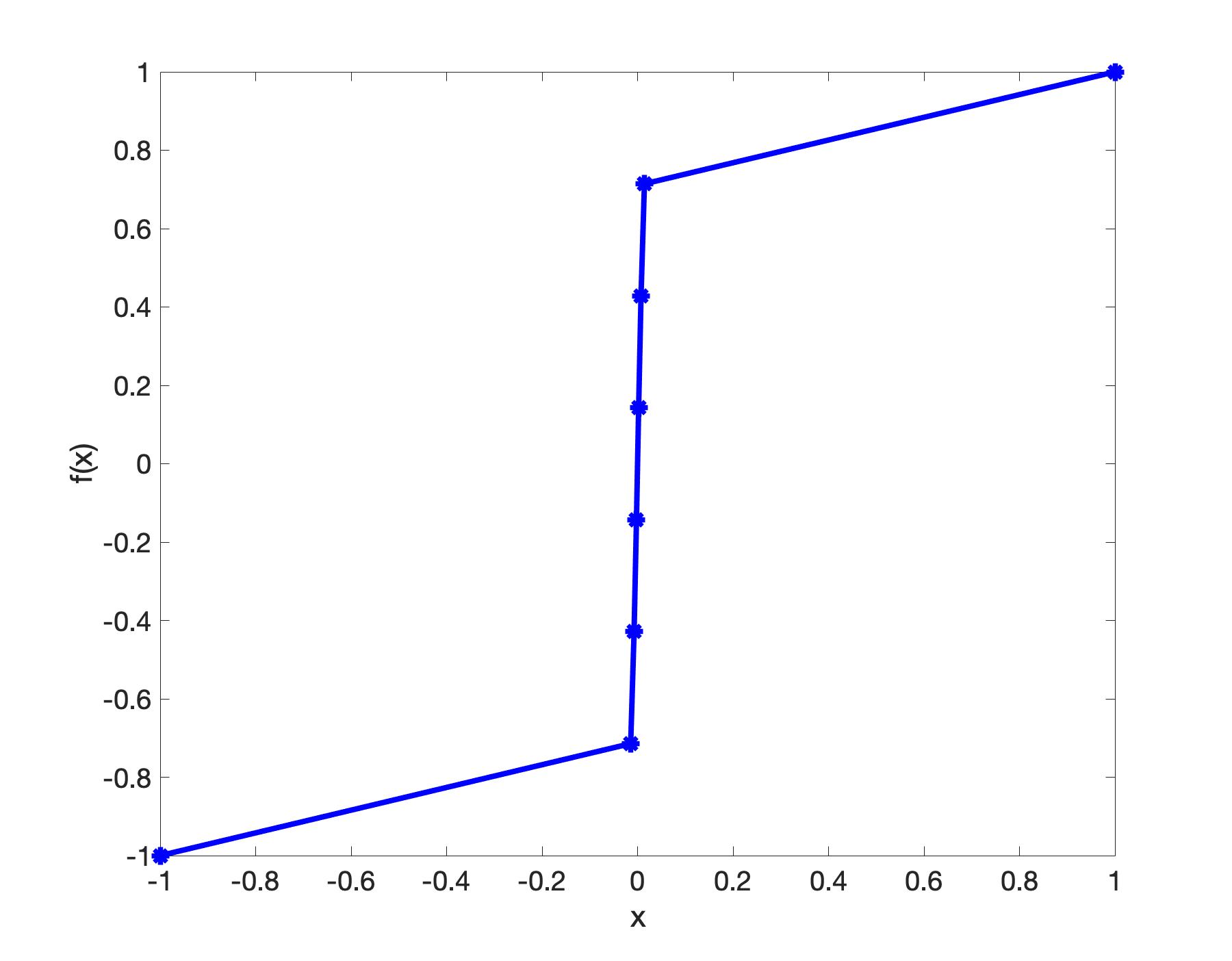
(e) $\epsilon^{2}=10^{-4}$ and $N=8$.

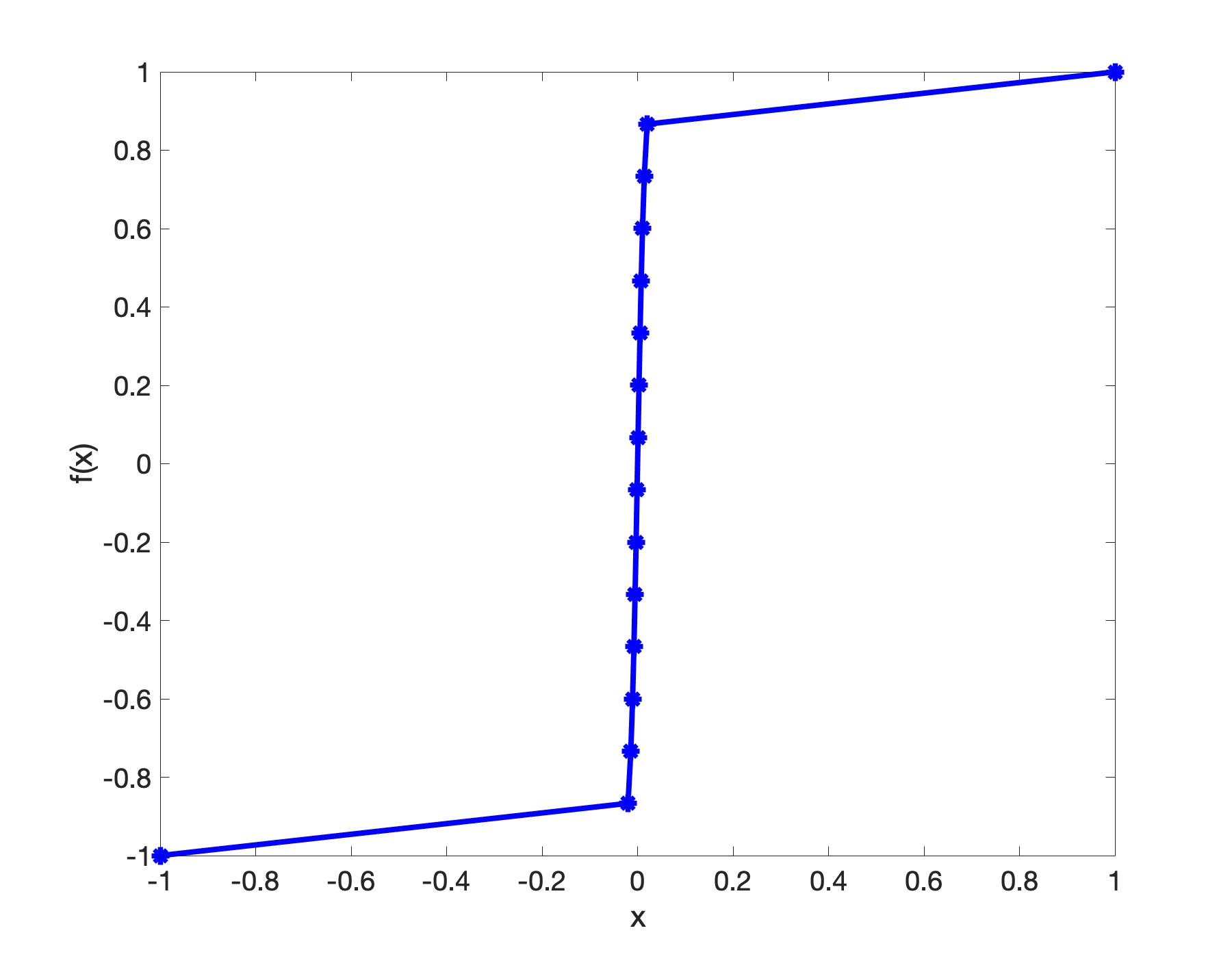
(f) $\epsilon^{2}=10^{-4}$ and $N=16$ .

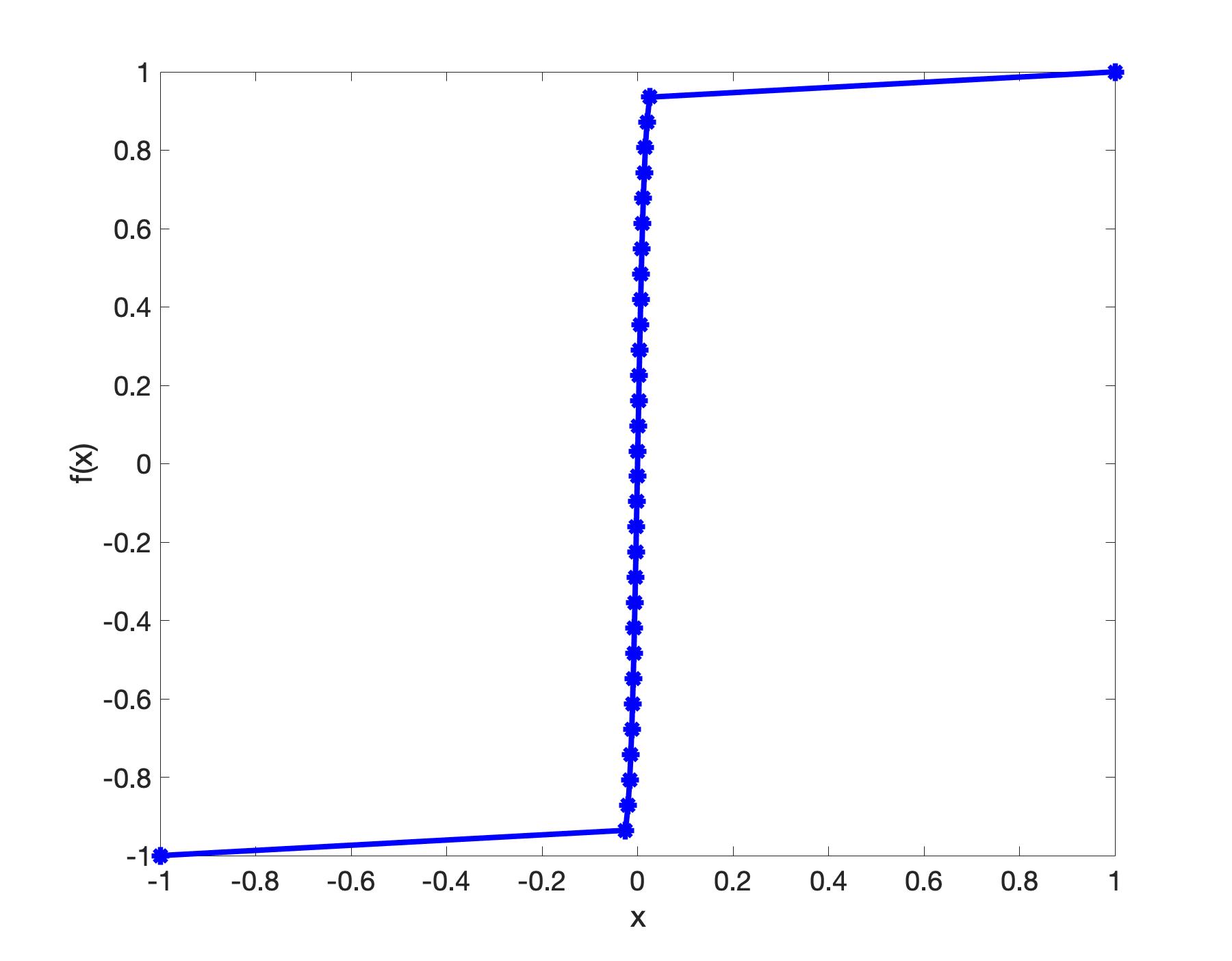
(g) $\epsilon^{2}=10^{-4}$ and $N=32$

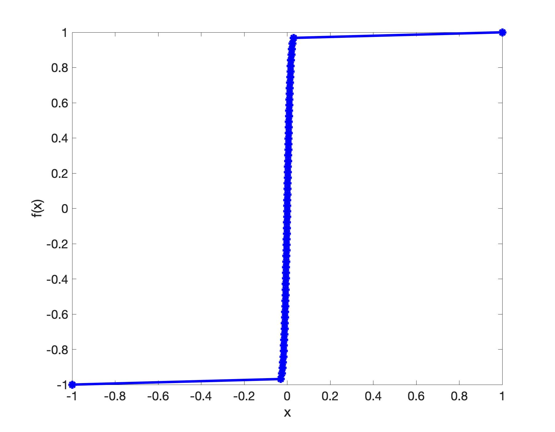
(h) $\epsilon^{2}=10^{-4}$ and $N=64$

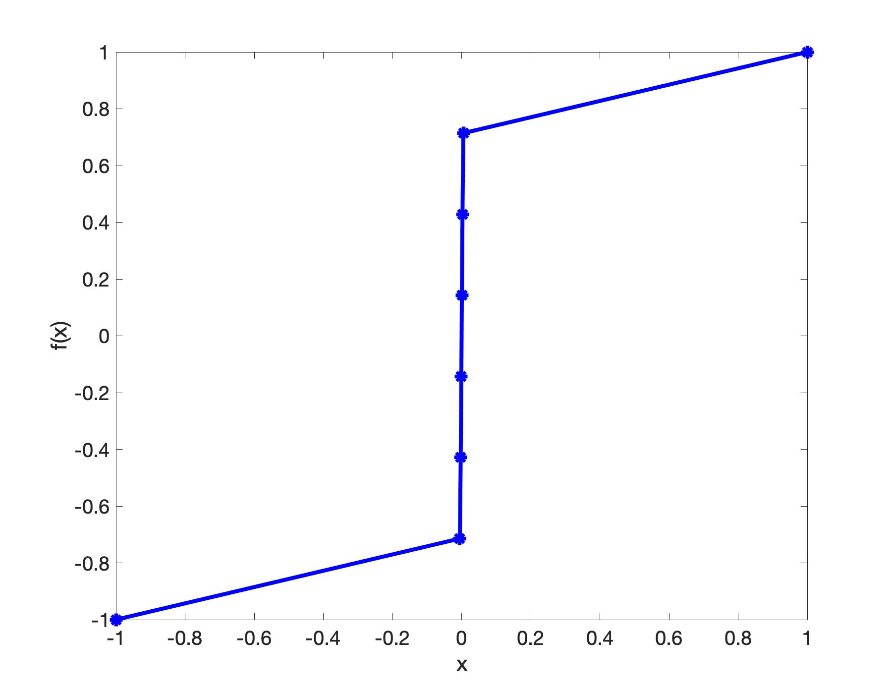
(i) $\epsilon^{2}=10^{-5}$ and $N=8$.

(j) $\epsilon^{2}=10^{-5}$ and $N=16$ .

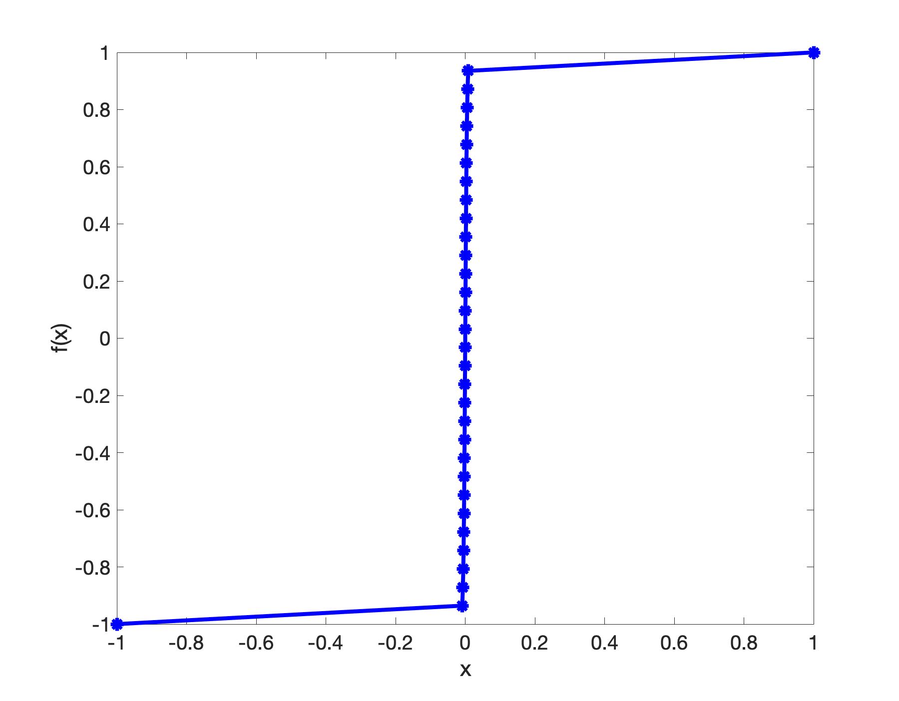
(k) $\epsilon^{2}=10^{-5}$ and $N=32$

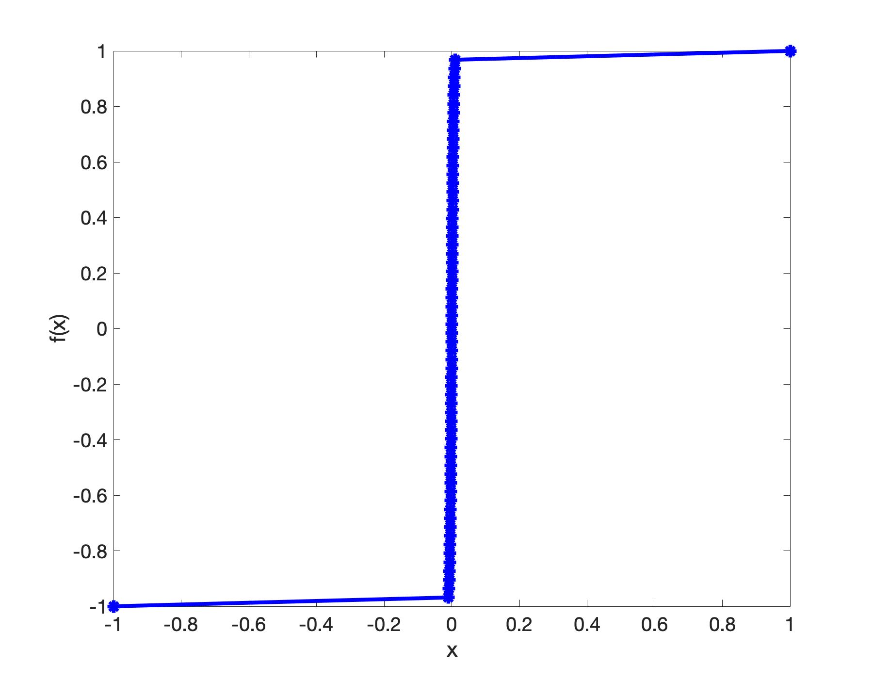
(l) $\epsilon^{2}=10^{-5}$ and $N=64$

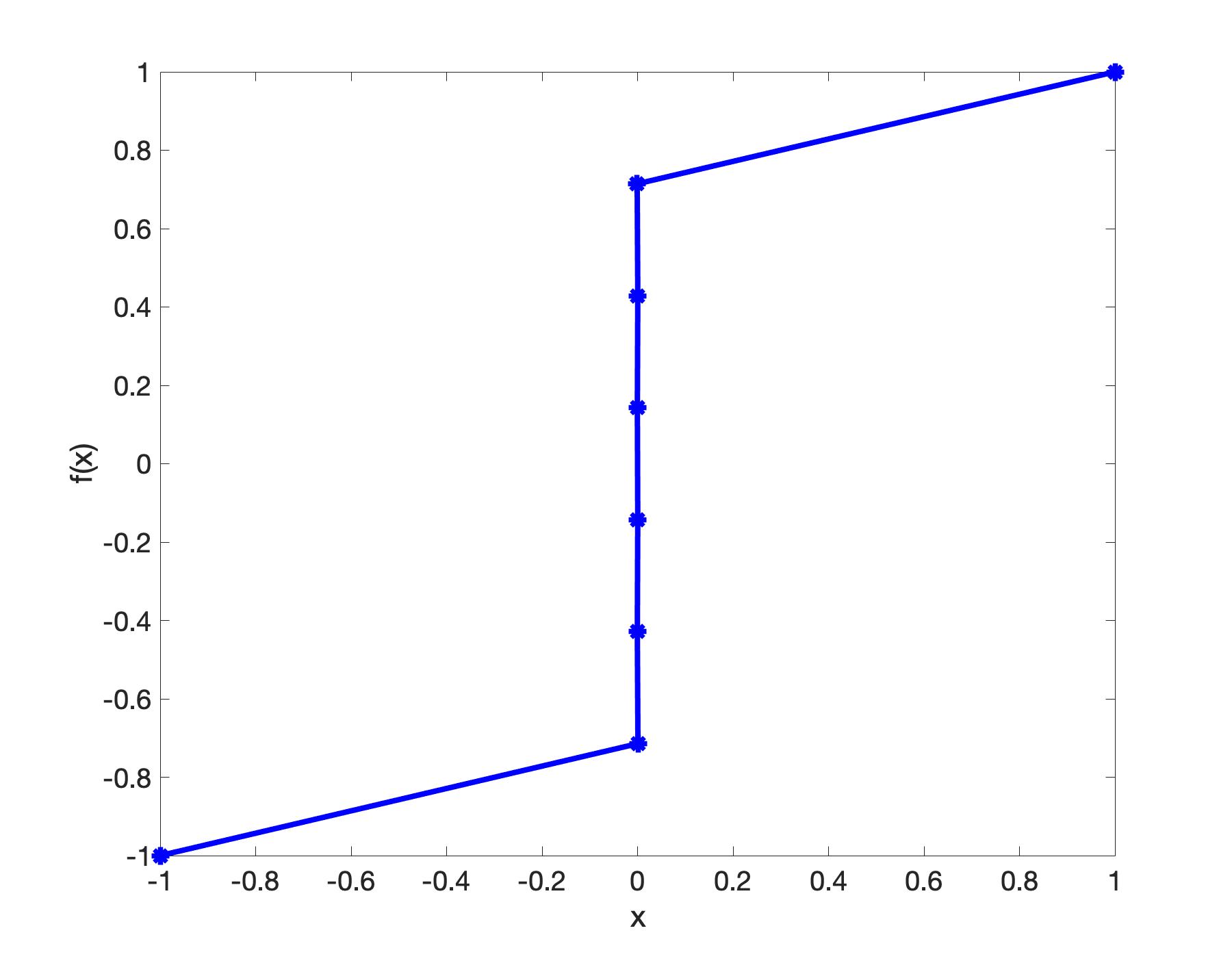
(m) $\epsilon^{2}=10^{-6}$ and $N=8$.

(n) $\epsilon^{2}=10^{-6}$ and $N=16$ .

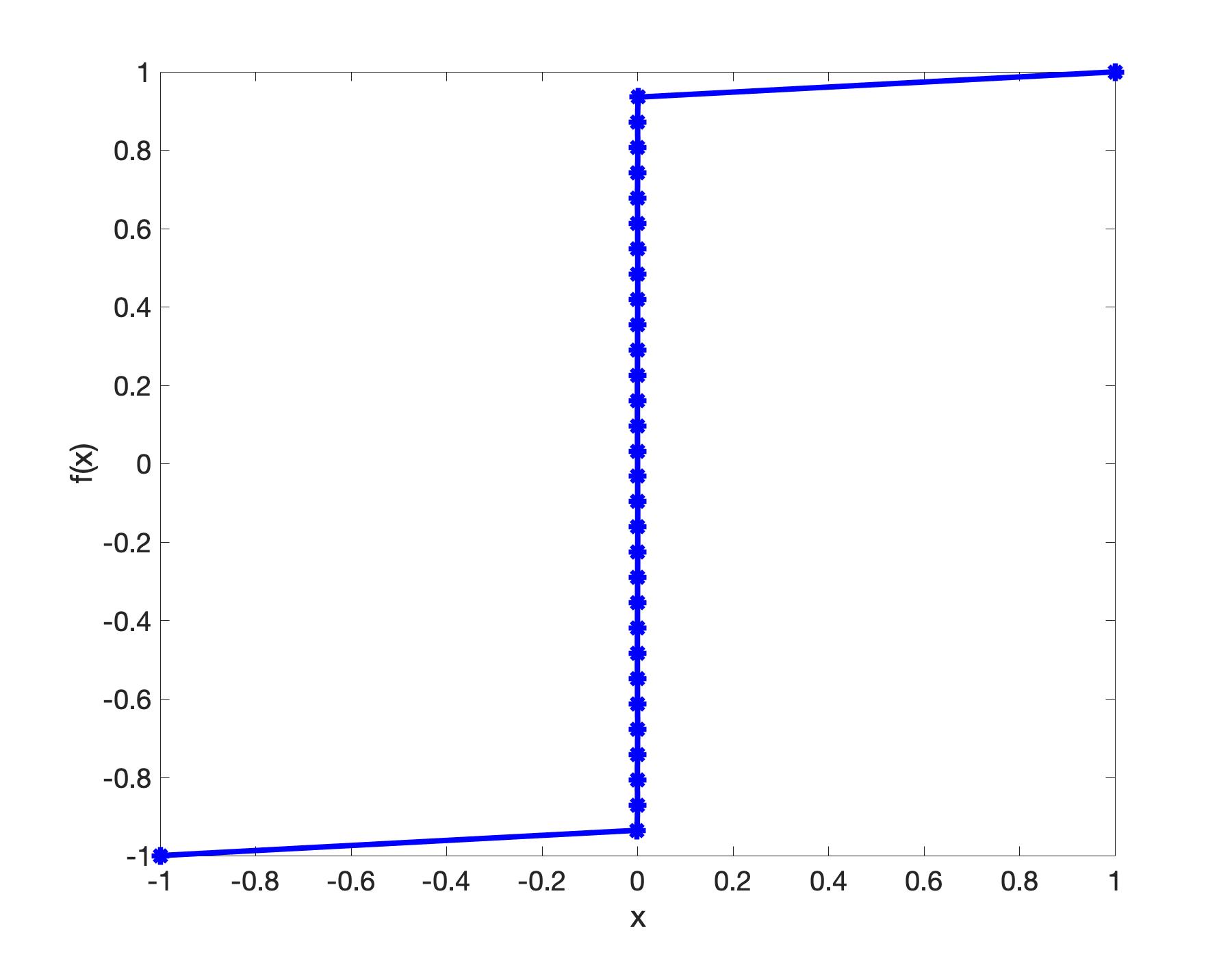
(o) $\epsilon^{2}=10^{-6}$ and $N=32$

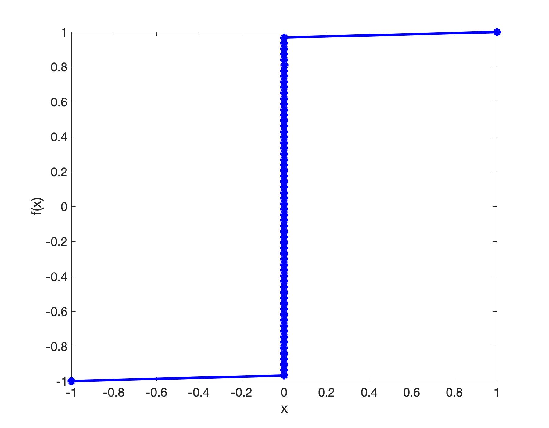
(p) $\epsilon^{2}=10^{-6}$ and $N=64$

Figure 4. Approximate steady states of Allen-Cahn equation by using the Lagrangian method with finite-element in space.

To obtain better approximation for both location and values of the interface, it is natural to consider the Lagrangian scheme with spectral method in space. In Fig. 7 and Fig. 8, we plot the results for $\epsilon^{2}=10^{-3}$ and $\epsilon^{2}=10^{-5}$ with $N=8,16,32,64$, respectively. We first look at the first and third column of the two figures. we observe that while most of the points are still located in the interfacial region, but the approximate solutions exhibit oscillations except at the finest resolution with $N=64$. This is a common phenomena with under-resolved spectral methods. Usually this can be fixed with a suitable filter to post-process the oscillatory approximate solutions [33, 18].

Hence, in order to remove the oscillation, we use an exponential filter for post-processing. More precisely, given approximate solution $u_{N}=\sum\limits_{n=0}^{N}\hat{u}_{n}L_{n}(x)$ with $L_{n}(x)$ being the Legendre polynomial of degree $n$, we set the filtered solution to be

(5.3) $$F_{N}u_{N}=\sum\limits_{n=0}^{N}\sigma(\frac{n}{N})\hat{u}_{n}L_{n}(x),$$

where $\sigma(\frac{n}{N})=\exp(-a(\frac{n}{N}))$, and $a=-\log(\epsilon_{M})$ where $\epsilon_{M}$ is the machine accuracy. The filtered results are presented in the second and fourth columns of Figs. 7 and Fig. 8. We observe that the filtered solutions are non-oscillatory and approximate the exact solutions much better than the finite-element methods. In fact, while the values with $N=8$ are still visibly different from the exact solution, excellent approximations are obtained with $N=16$ for both cases.

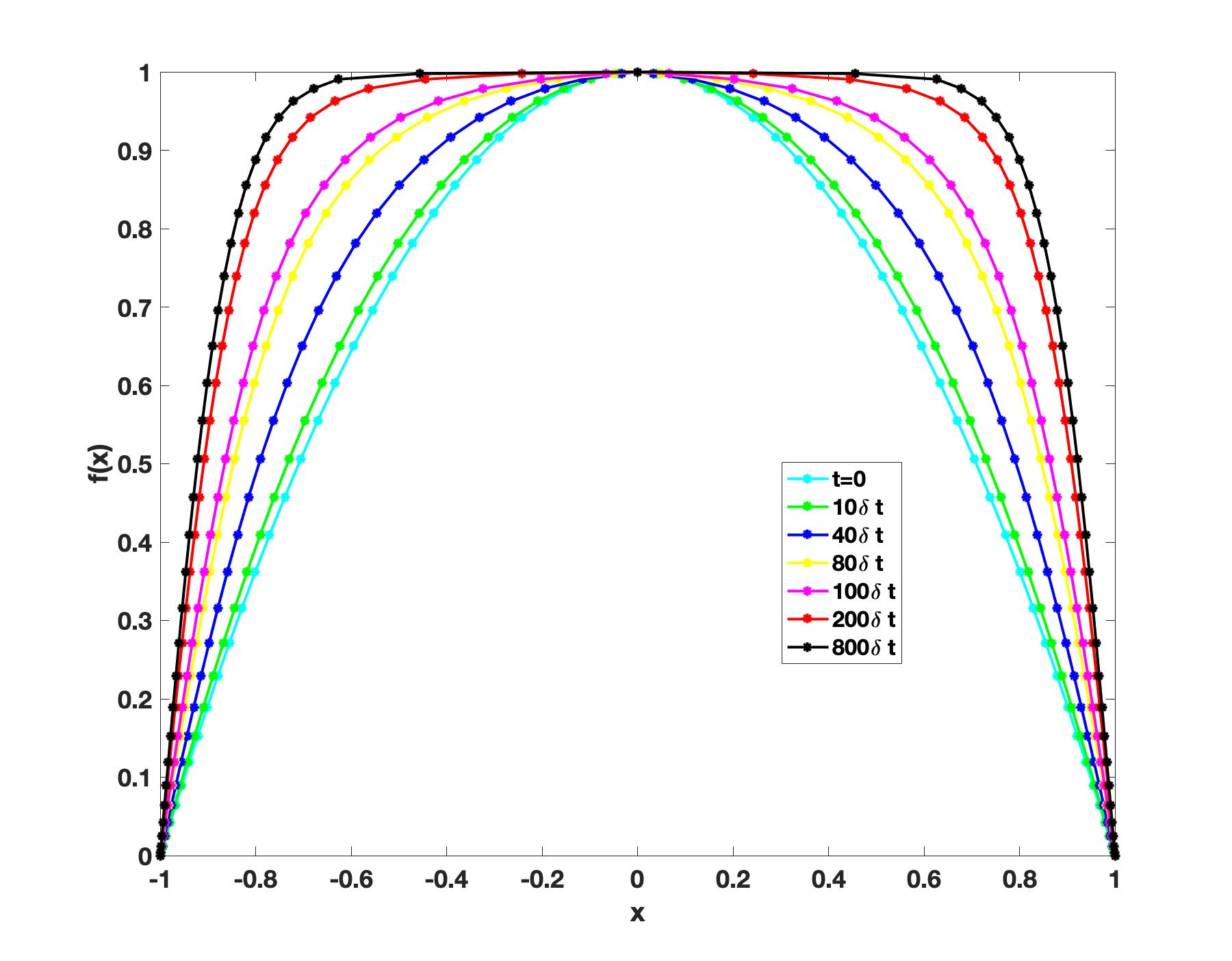
(a) Flow dynamic approach with Spectral method: $N=64$, $\epsilon^{2}=0.01$.

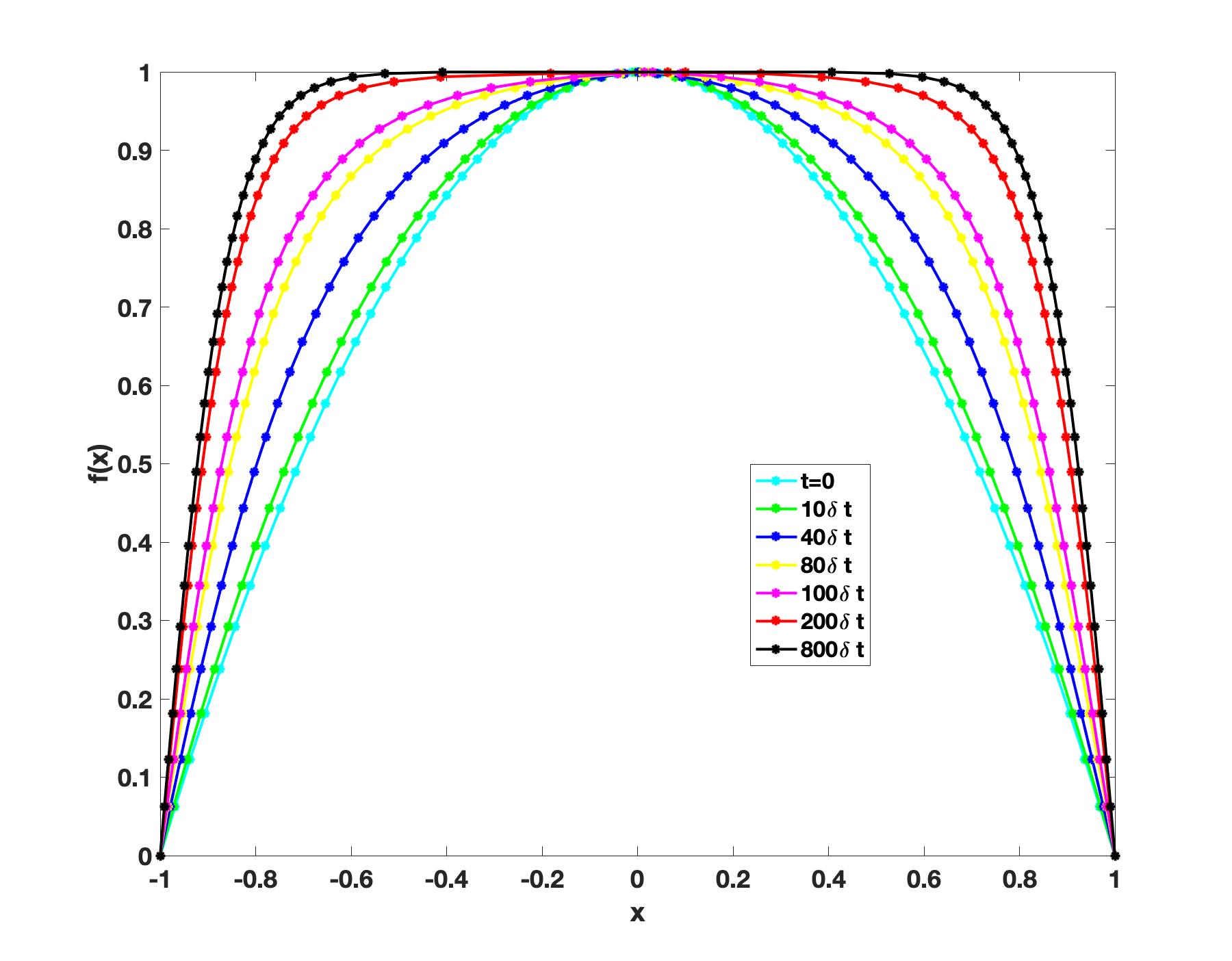
(b) Flow dynamic approach with Finite element method: $N=64$, $\epsilon^{2}=0.01$.

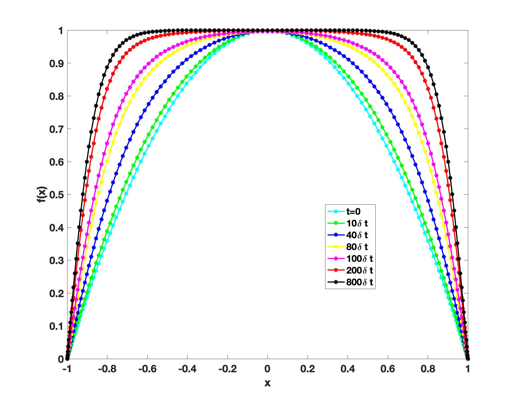
(c) Numerical method in Eulerian coordinate $N=128$ and $\epsilon^{2}=0.01$ .

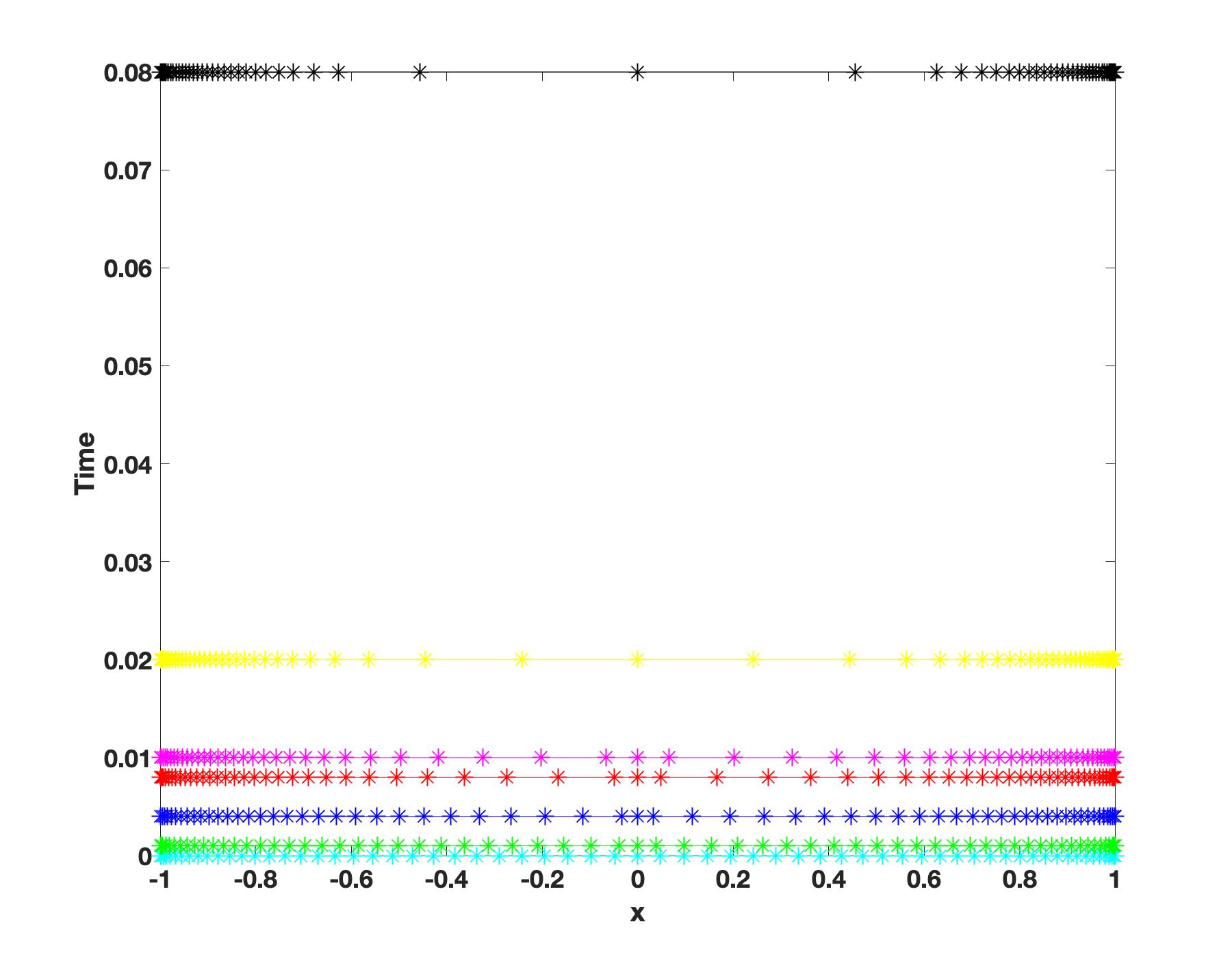
(d) Mesh distribution for Flow dynamic approach.

Figure 5. Capturing interface by Lagrangian numerical method based on Variational Energetic Approach.

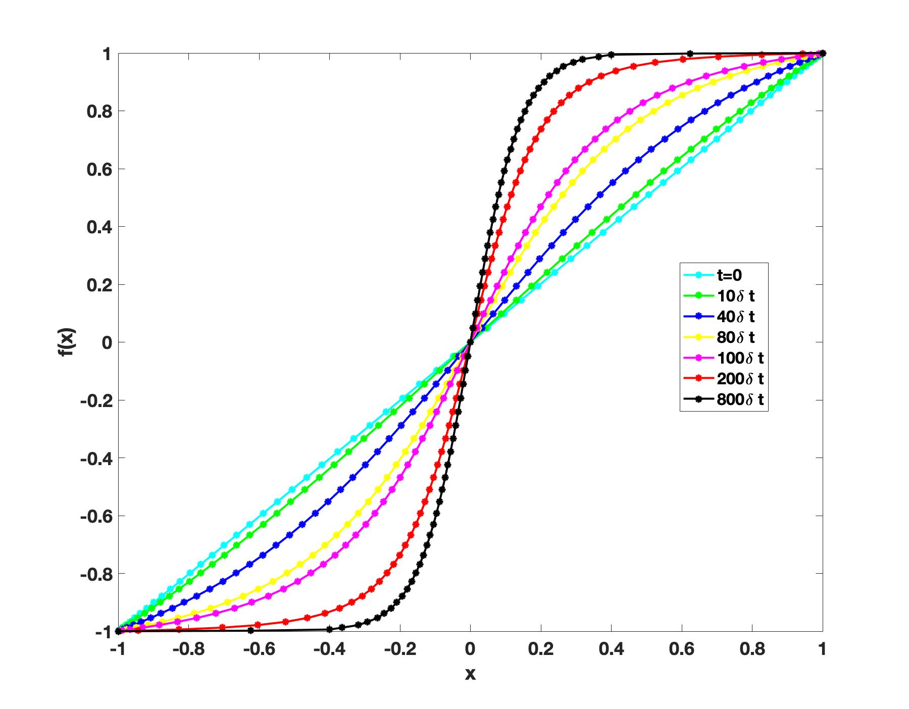
(a) Flow dynamic approach with Spectral method, $N=64$, $\epsilon^{2}=0.01$.

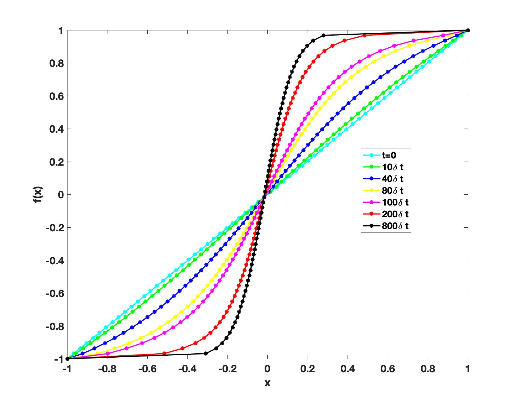
(b) Flow dynamic approach with finite element method, $N=64$, $\epsilon^{2}=0.01$.

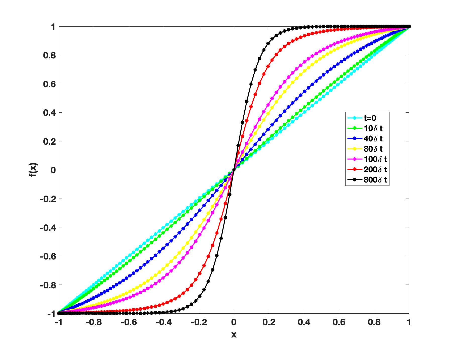
(c) Numerical method in Eulerian coordinate $N=128$ and $\epsilon^{2}=0.01$ .

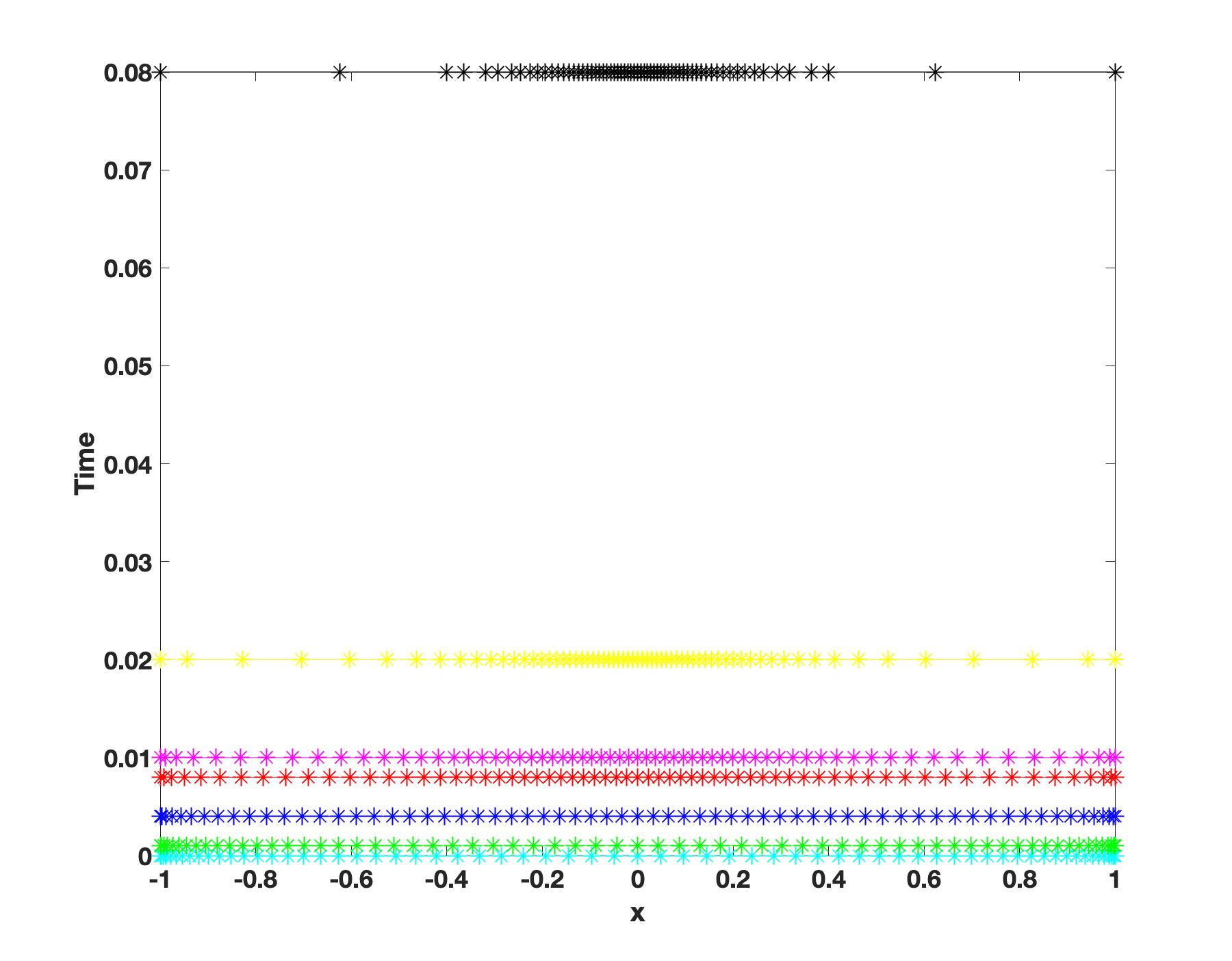
(d) Mesh distribution for Moving mesh method

Figure 6. Capturing interface by Lagrangian numerical method based on Variational Energetic Approach.

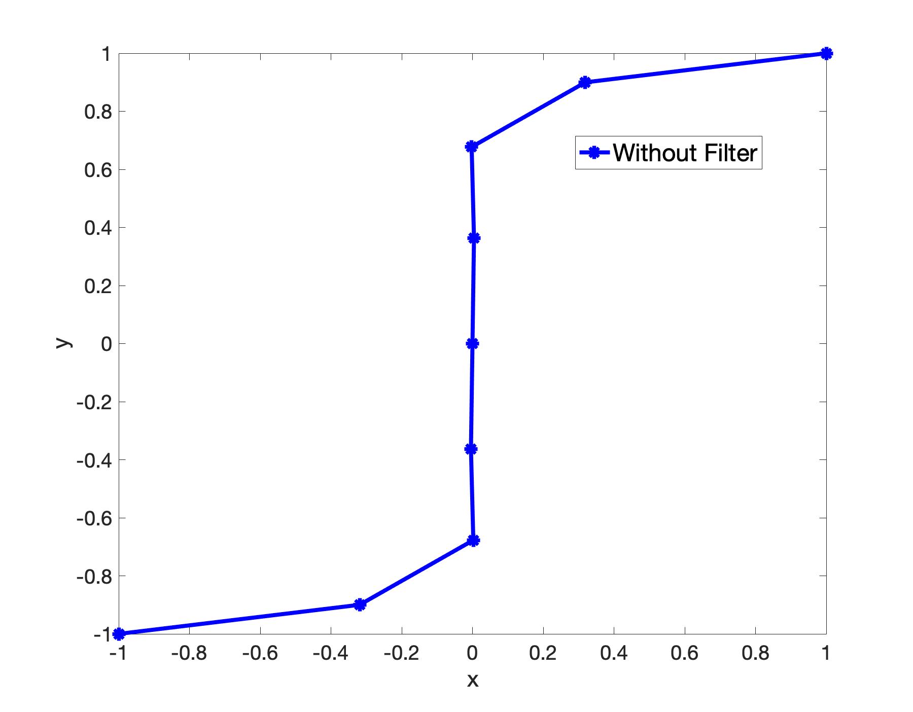
(a) $\epsilon^{2}=10^{-3}$ and $N=8$ without spectral filter.

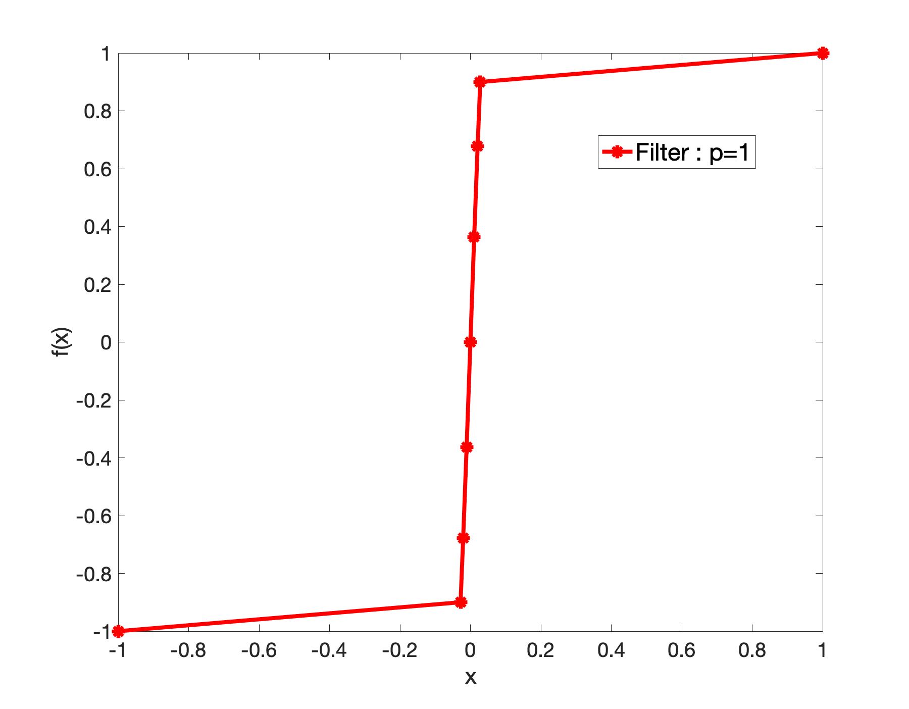
(b) $\epsilon^{2}=10^{-3}$ and $N=8$ with spectral filter .

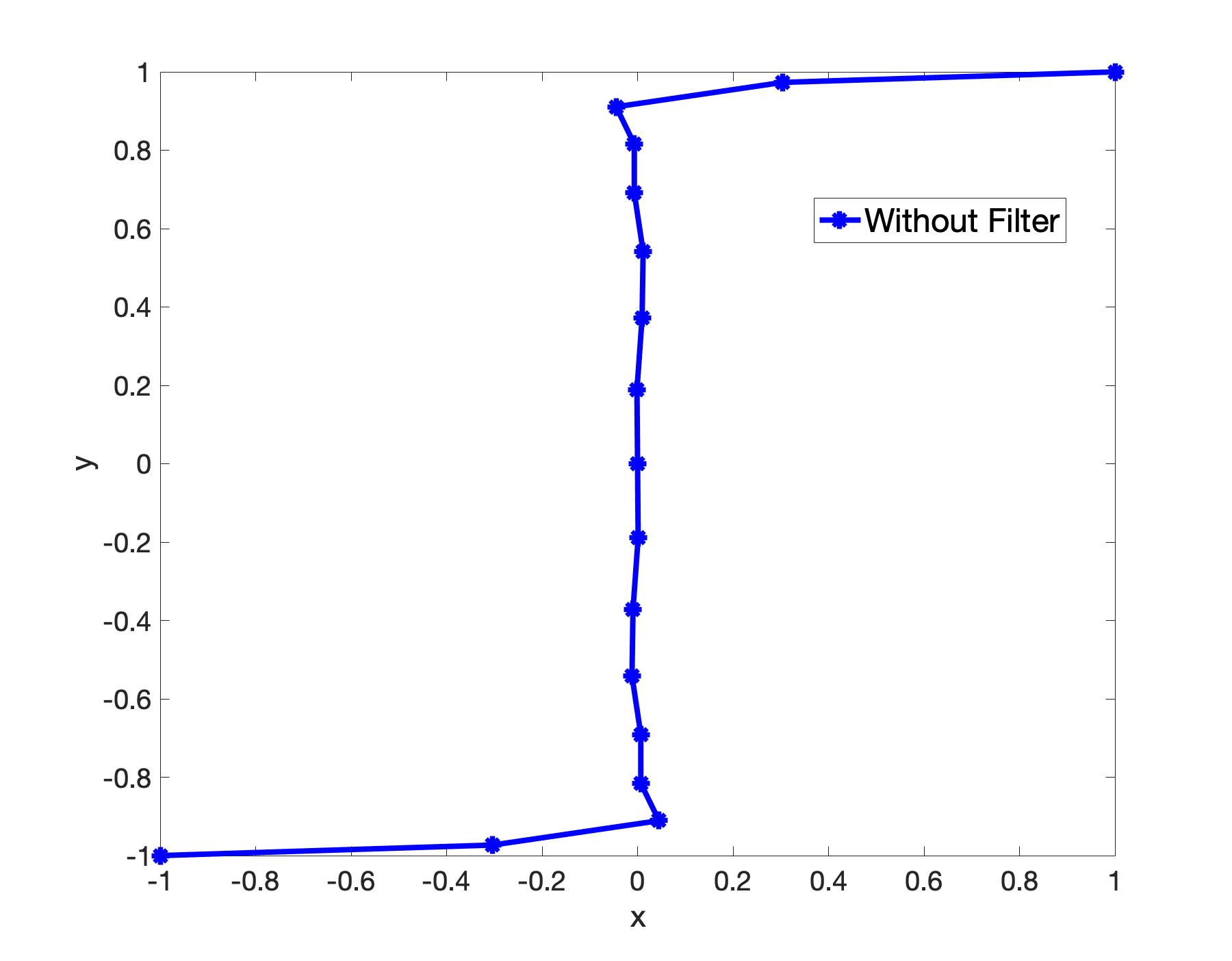
(c) $\epsilon^{2}=10^{-3}$ and $N=16$ without spectral filter.

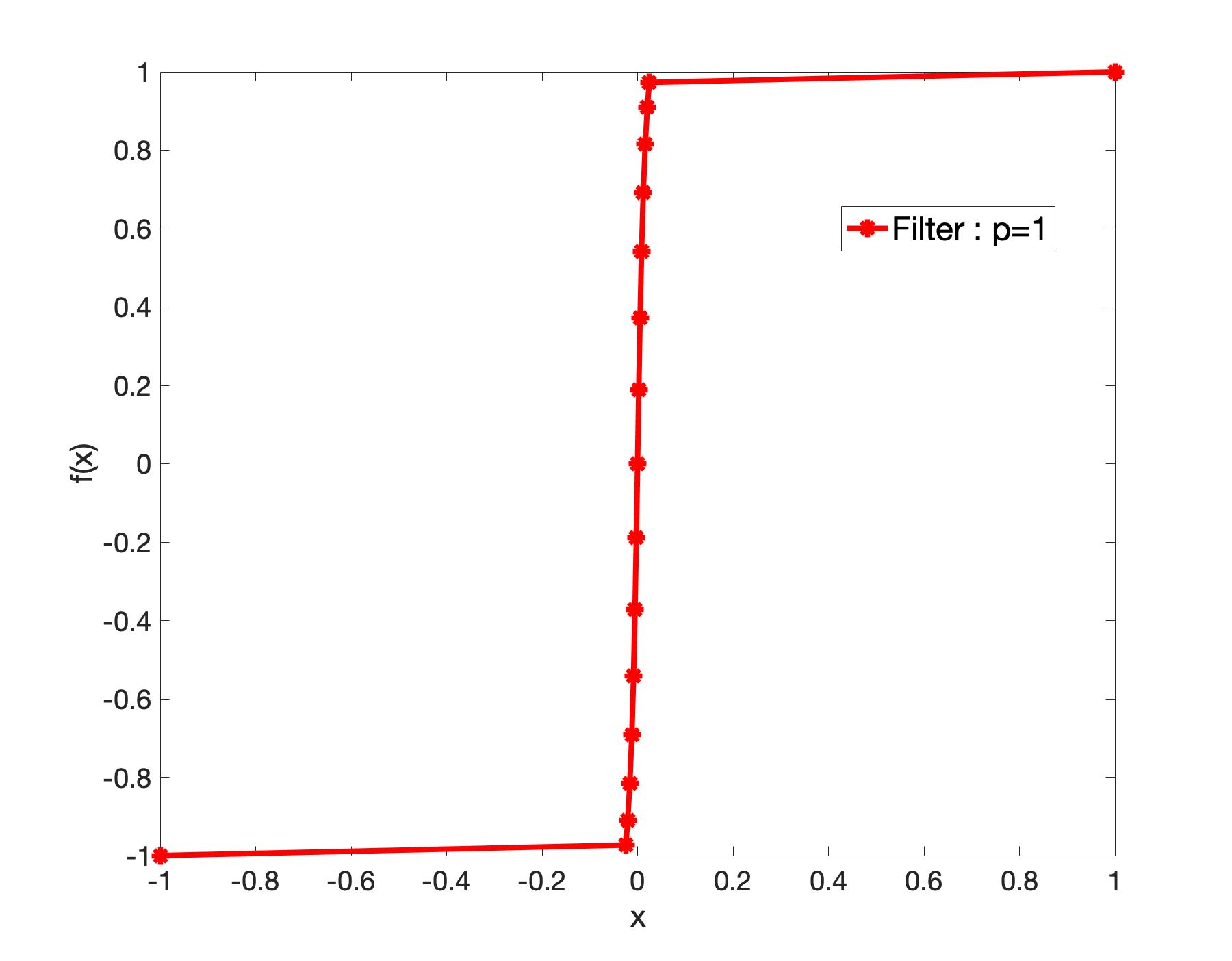
(d) $\epsilon^{2}=10^{-3}$ and $N=16$ with spectral filter.

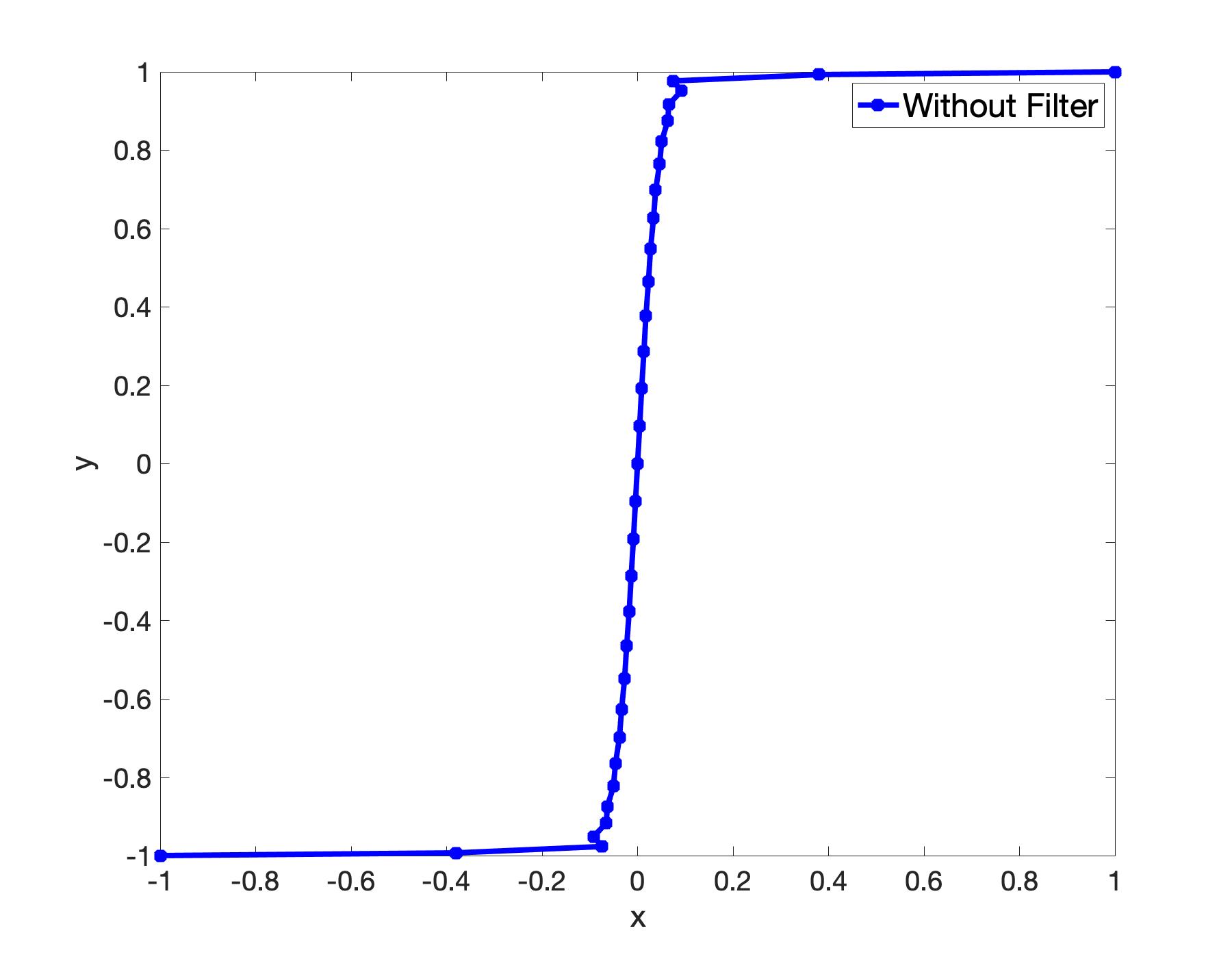
(e) $\epsilon^{2}=10^{-3}$ and $N=32$ without spectral filter.

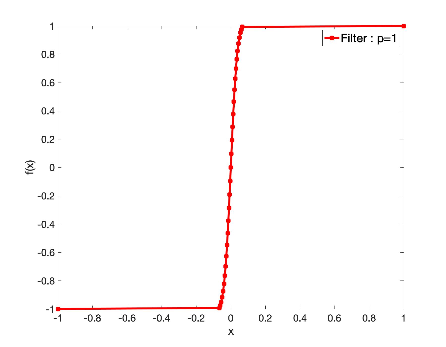
(f) $\epsilon^{2}=10^{-3}$ and $N=32$ with spectral filter.

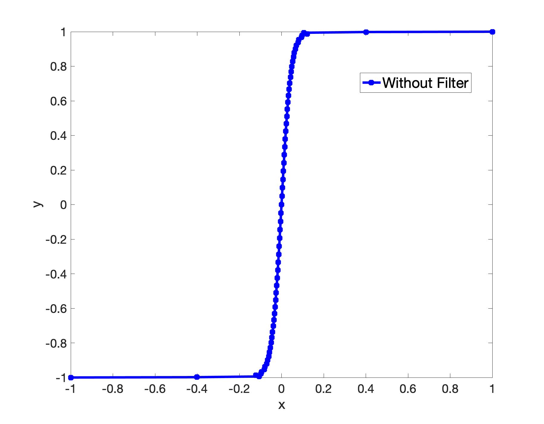
(g) $\epsilon^{2}=10^{-3}$ and $N=64$ without spectral filter.

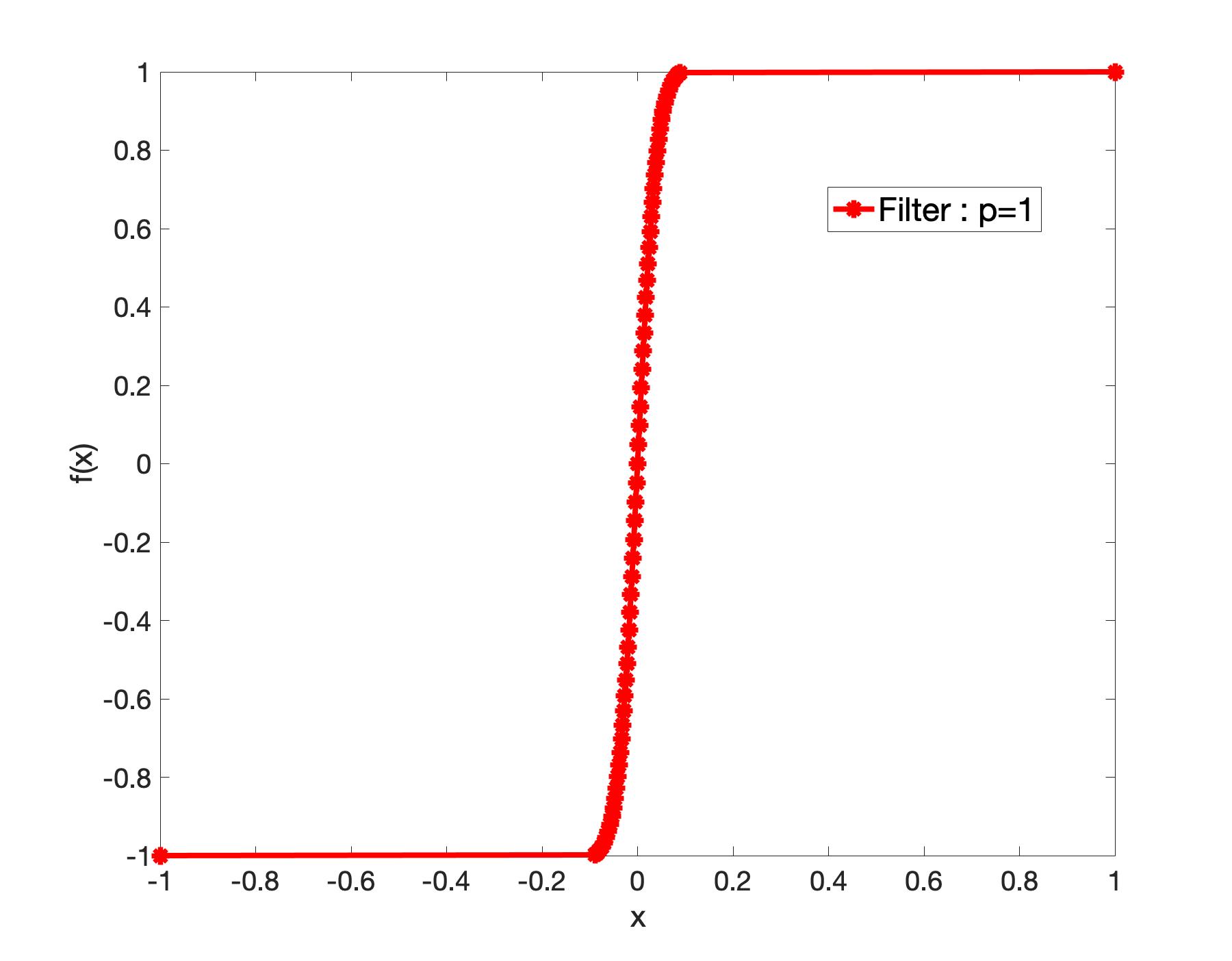
(h) $\epsilon^{2}=10^{-3}$ and $N=64$ with spectral filter.

Figure 7. Approximate steady states of Allen-Cahn equation by the Lagrangian scheme with Legendre Spectral method in space for $\epsilon^{2}=10^{-3}$.

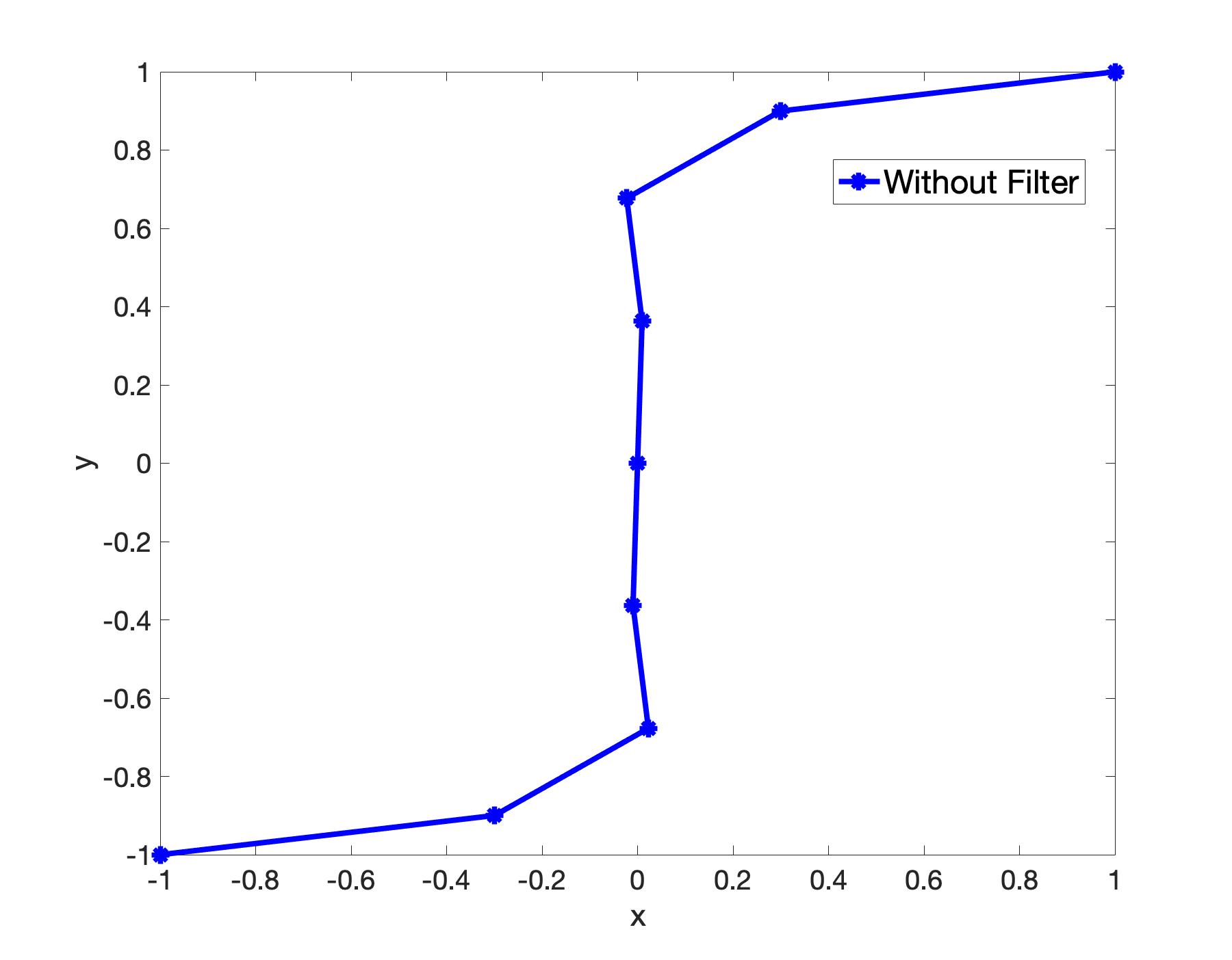
(a) $\epsilon^{2}=10^{-5}$ and $N=8$ without spectral filter.

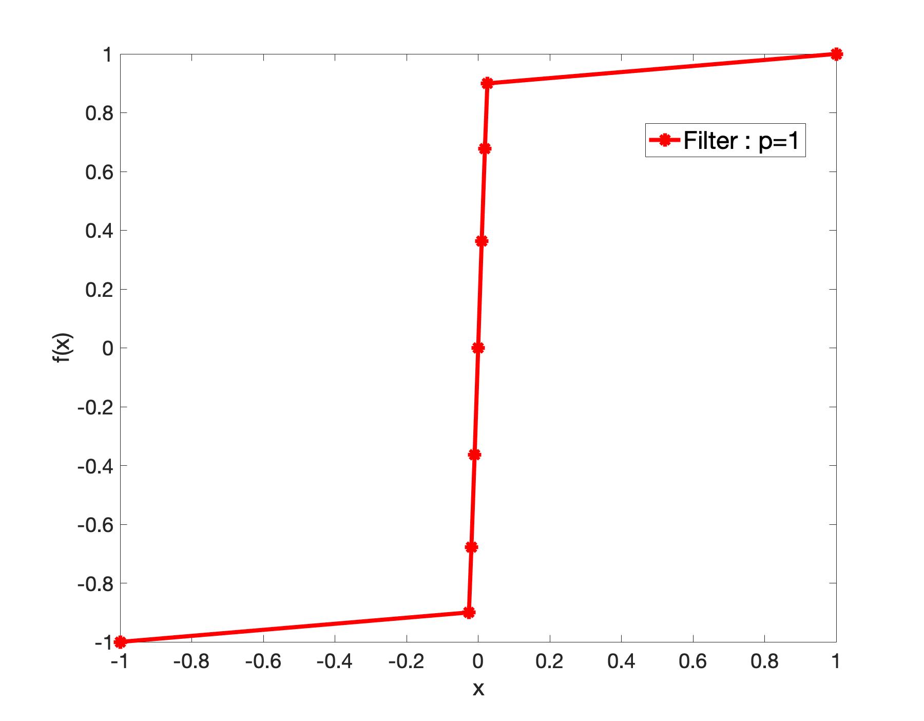
(b) $\epsilon^{2}=10^{-5}$ and $N=8$ with spectral filter .

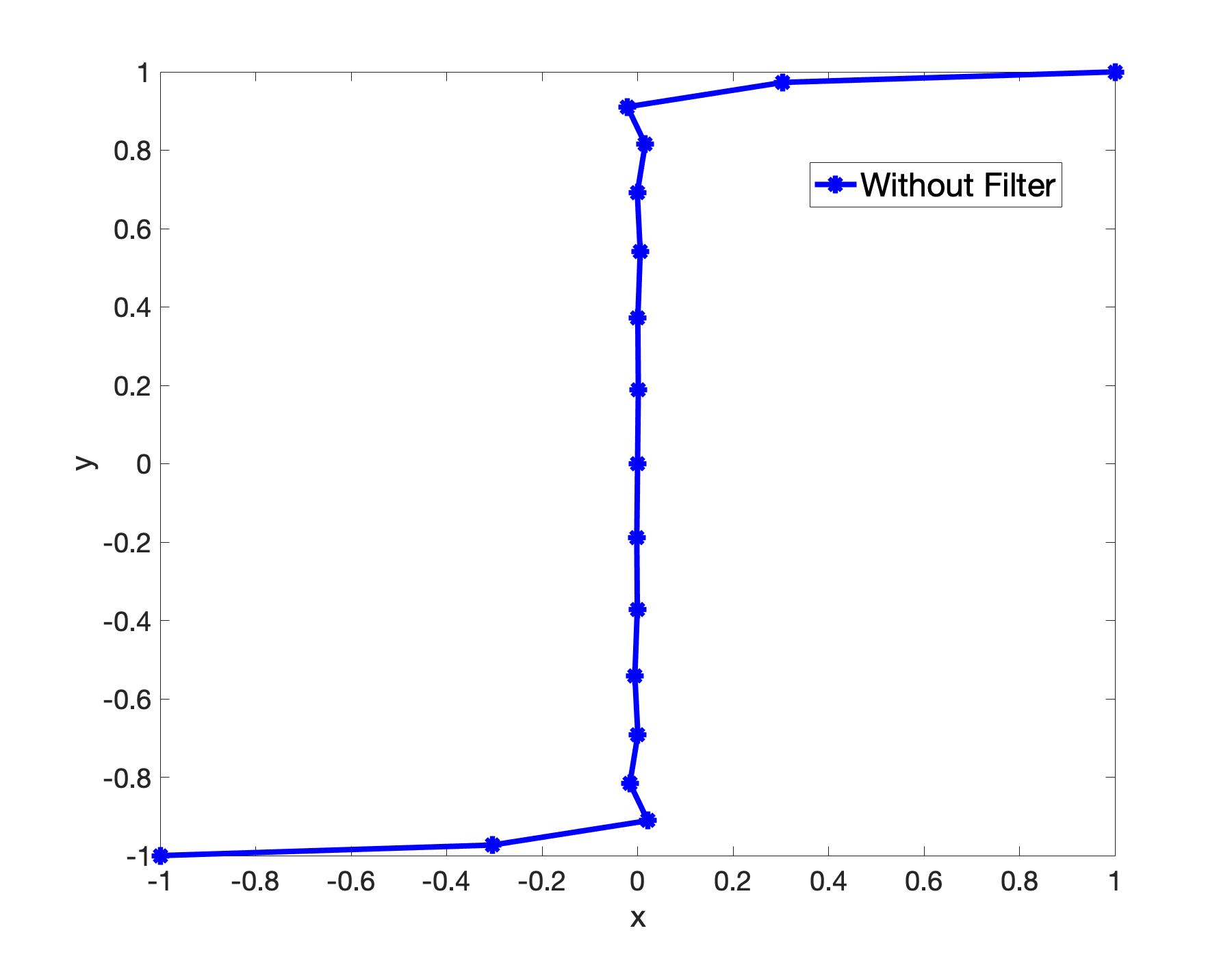
(c) $\epsilon^{2}=10^{-5}$ and $N=16$ without spectral filter.

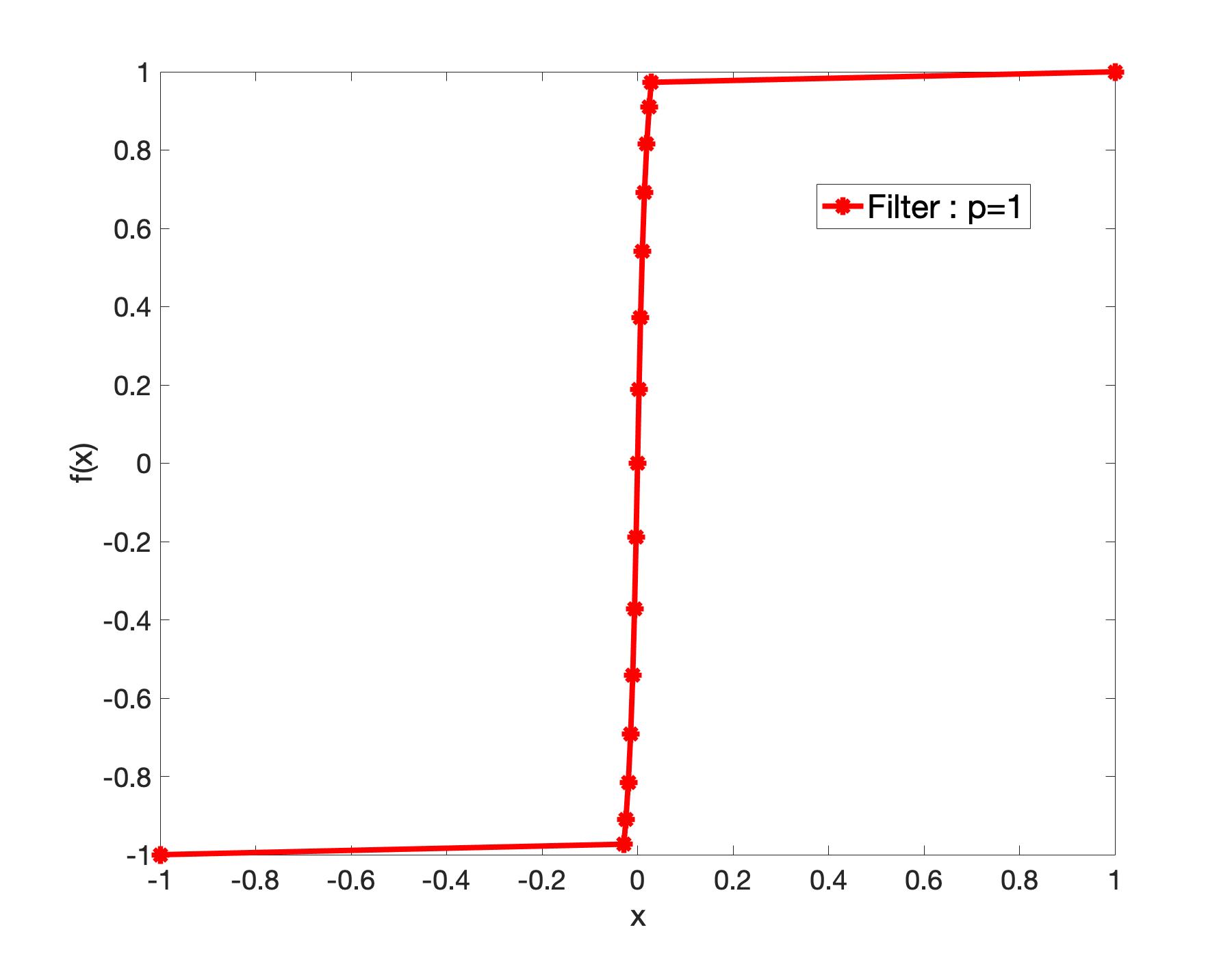
(d) $\epsilon^{2}=10^{-5}$ and $N=16$ with spectral filter.

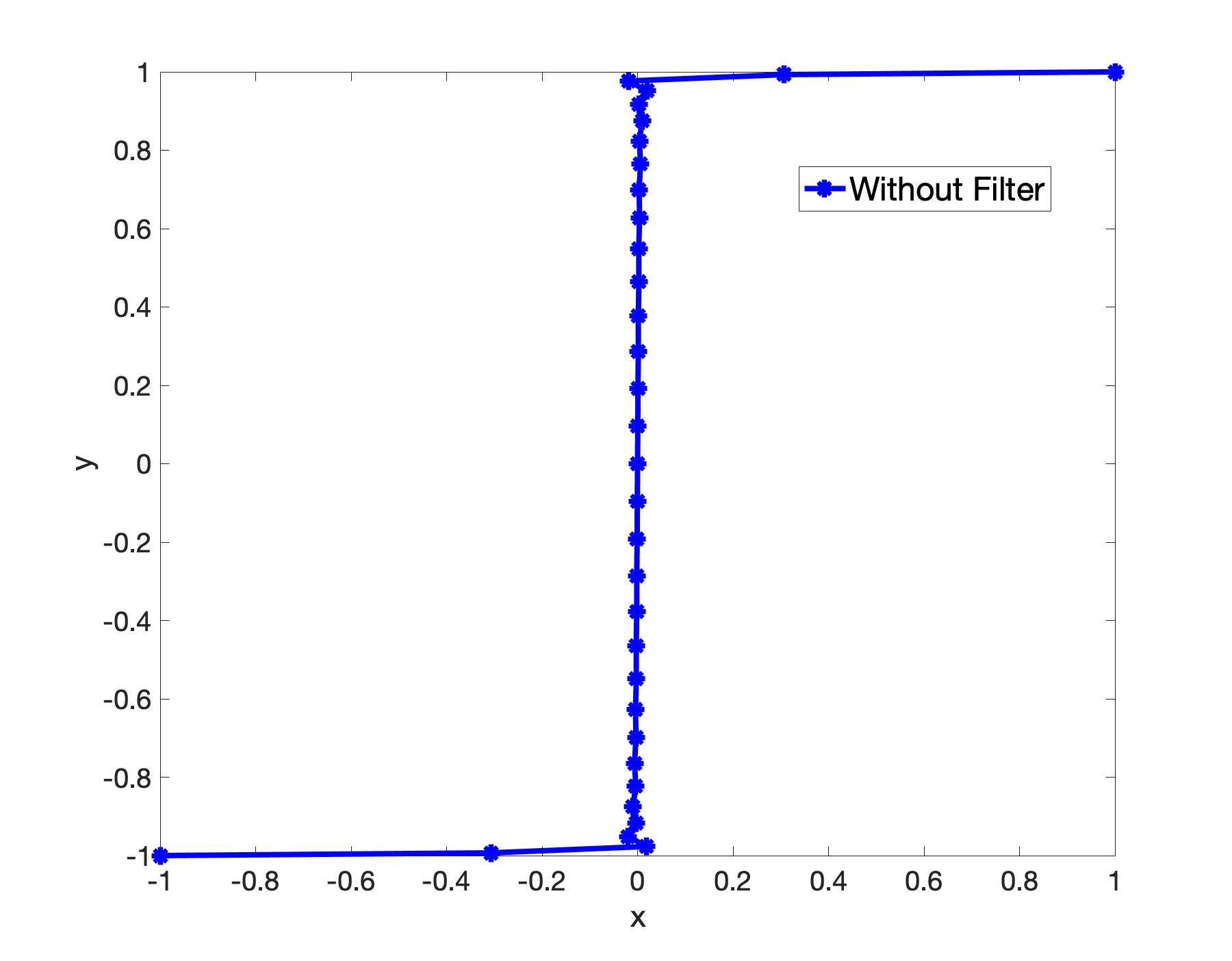
(e) $\epsilon^{2}=10^{-5}$ and $N=32$ without spectral filter.

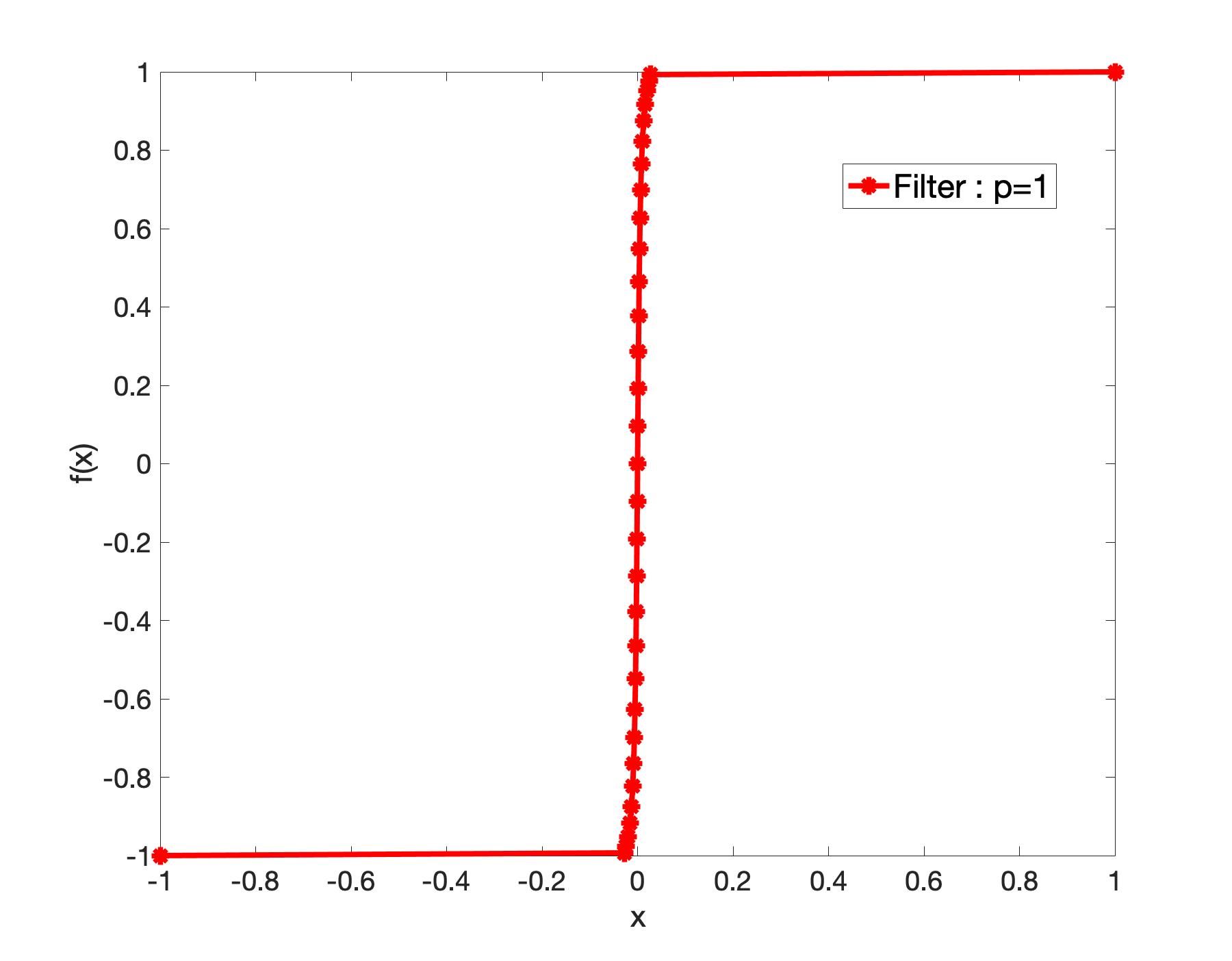
(f) $\epsilon^{2}=10^{-5}$ and $N=32$ with spectral filter.

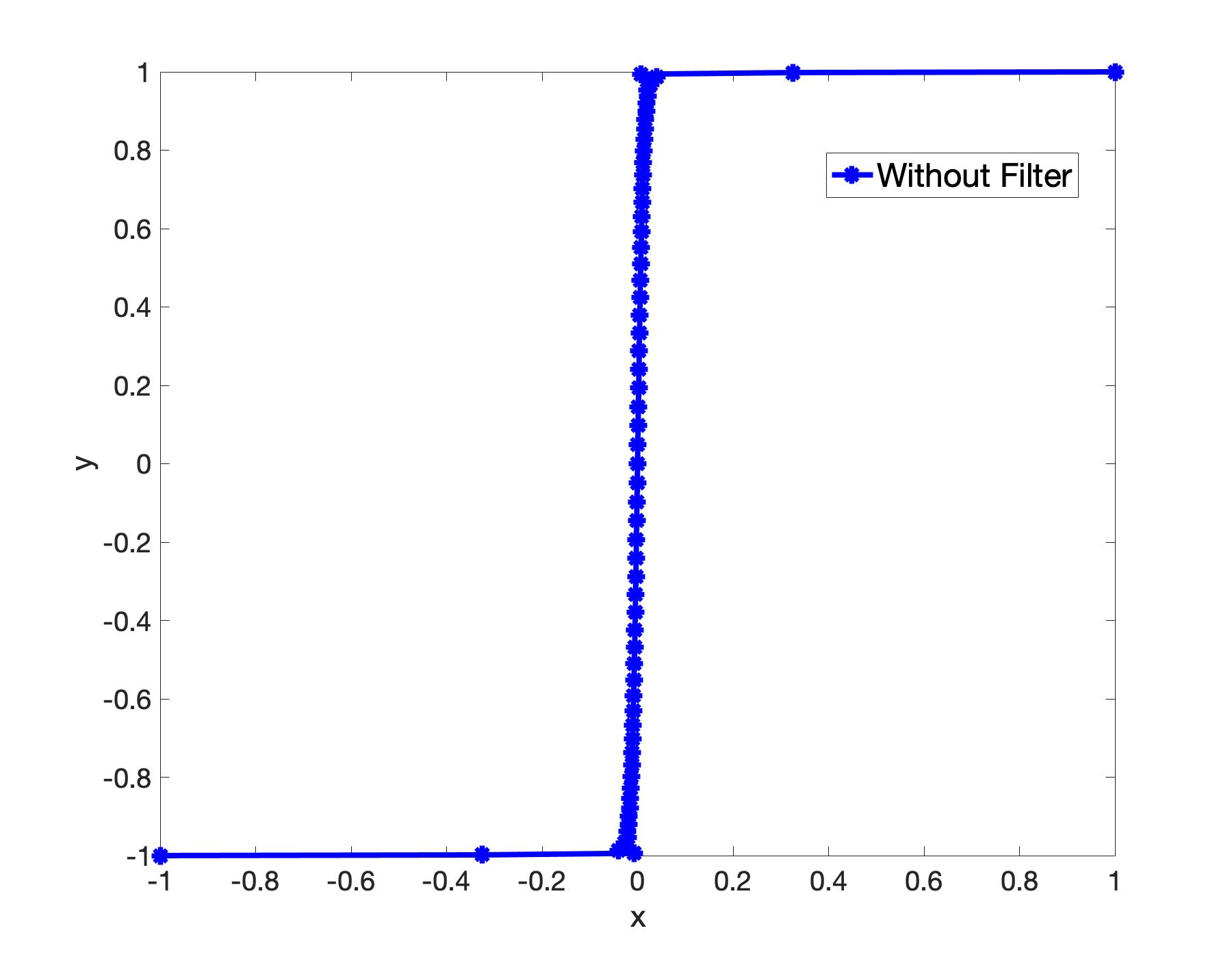
(g) $\epsilon^{2}=10^{-5}$ and $N=64$ without spectral filter.

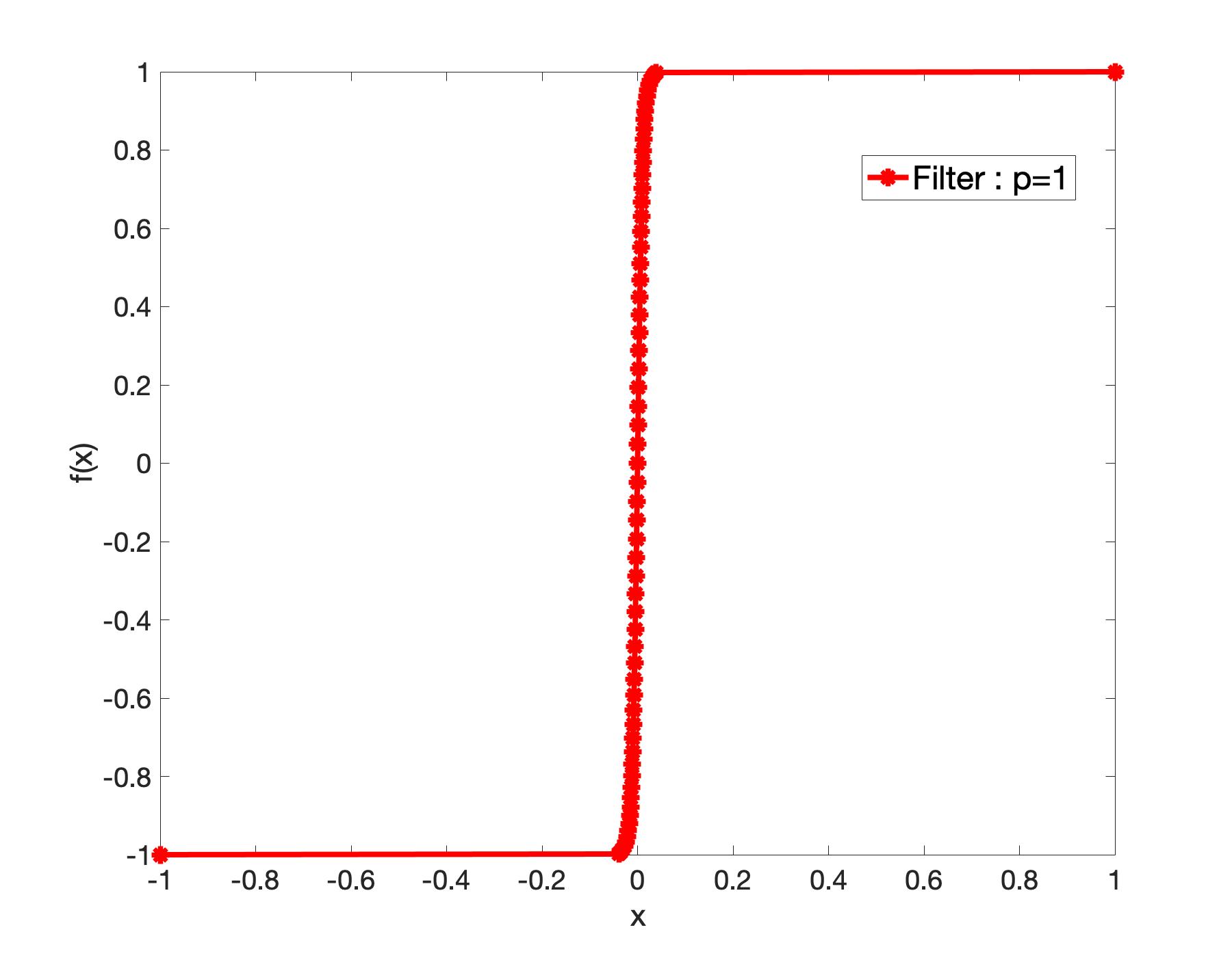
(h) $\epsilon=10^{-5}$ and $N=64$ with spectral filter.

Figure 8. Approximate steady states of Allen-Cahn equation by the Lagrangian scheme with Legendre Spectral method in space for $\epsilon^{2}=10^{-5}$.

Next, we consider the generalized Allen-Cahn equation (4.1) with an advection velocity ${\mathbf{v}}\equiv 1$, so the interface will evolve and move to the right. We would like to see how our Lagrangian method performs with moving interfaces. In Fig. 9 we plot the interface profiles at various times computed by the Lagrangian scheme with spectral method and finite element method in space for the generalized Allen-Cahn equation (4.1) with ${\mathbf{v}}\equiv 1$. As a comparison, we also plotted results by using a semi-implicit method in Eulerian coordinate. We observe that as the interface moves, our Lagrangian method can still capture the interface well with few points.

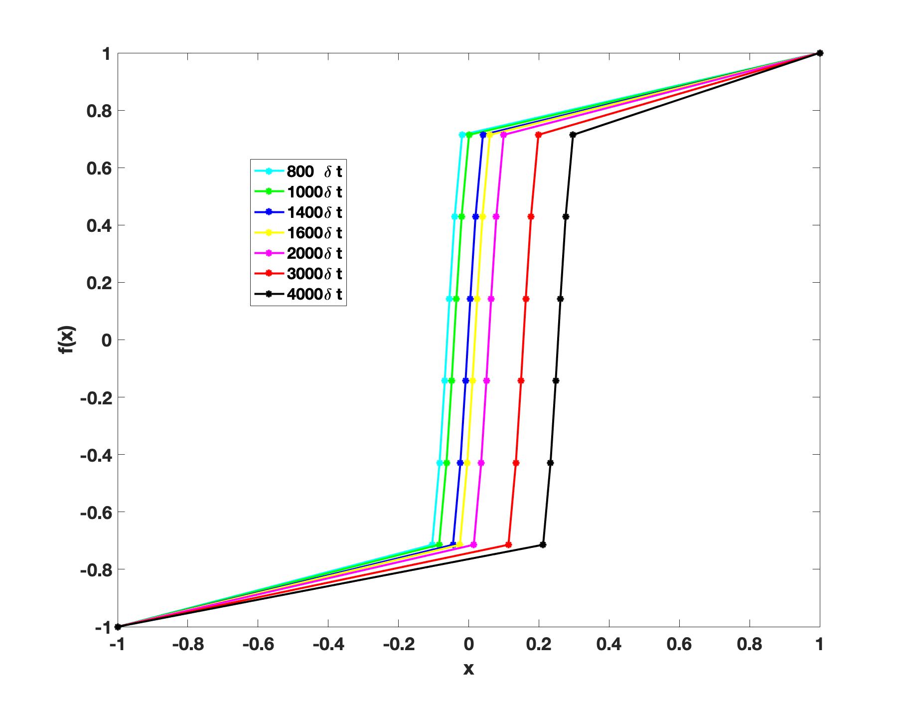
(a) Flow dynamic approach with Finite element method, $\epsilon^{2}=0.001$, $N=8$.

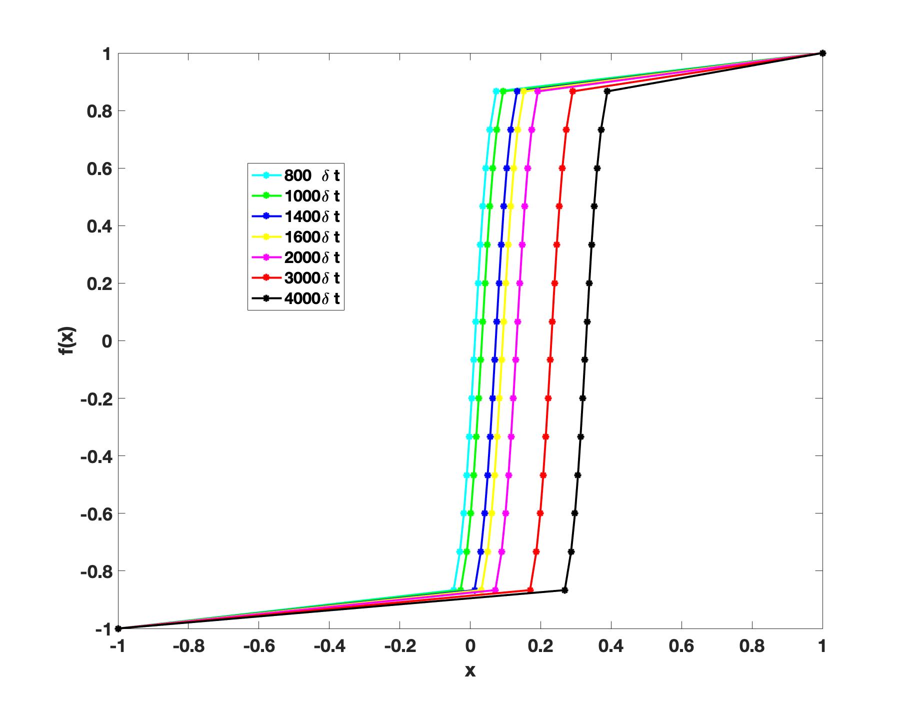
(b) Flow dynamic approach with Finite element method, $\epsilon^{2}=0.001$, $N=16$.

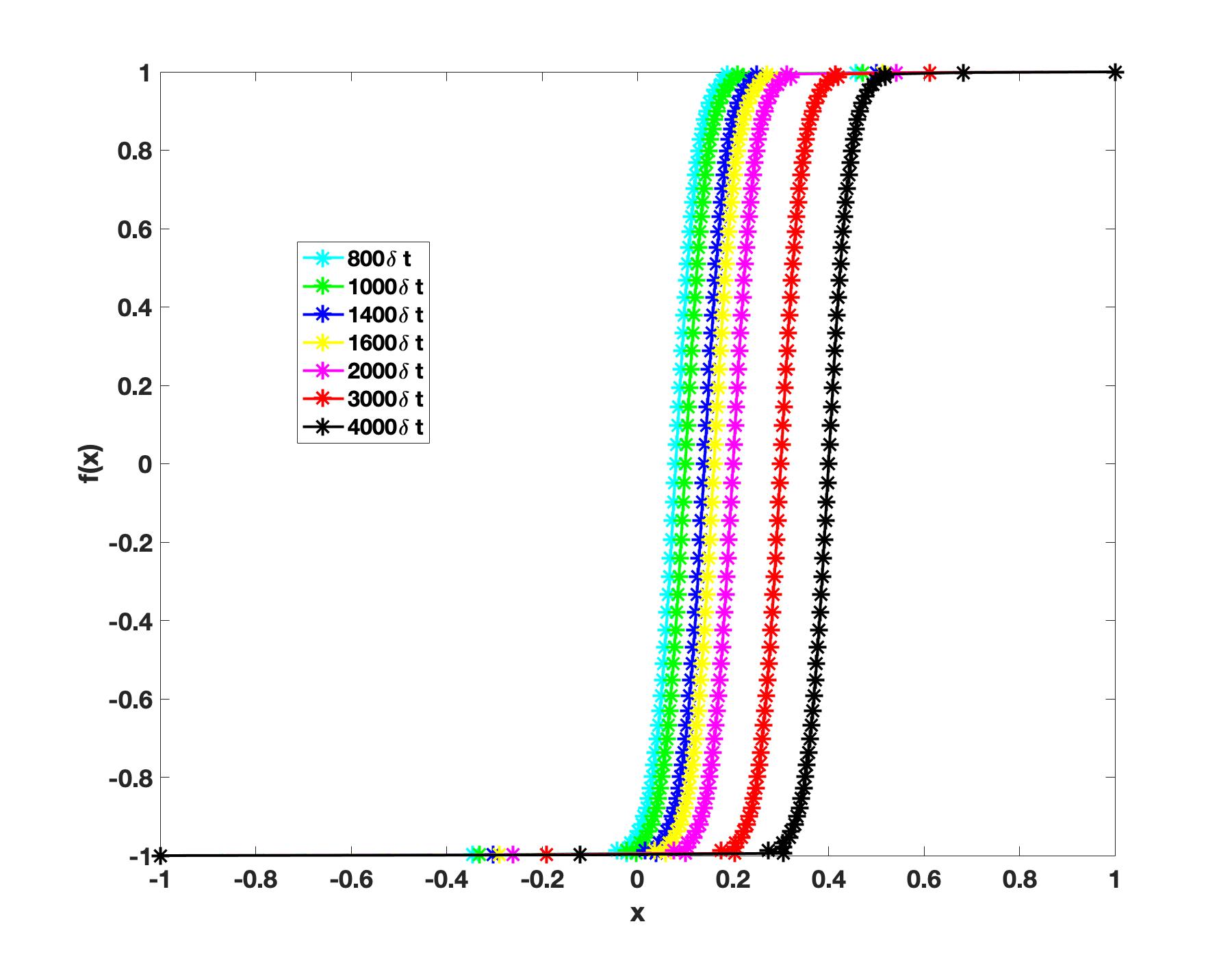
(c) Flow dynamic approach with Spectral method, $\epsilon^{2}=0.001$, $N=64$.

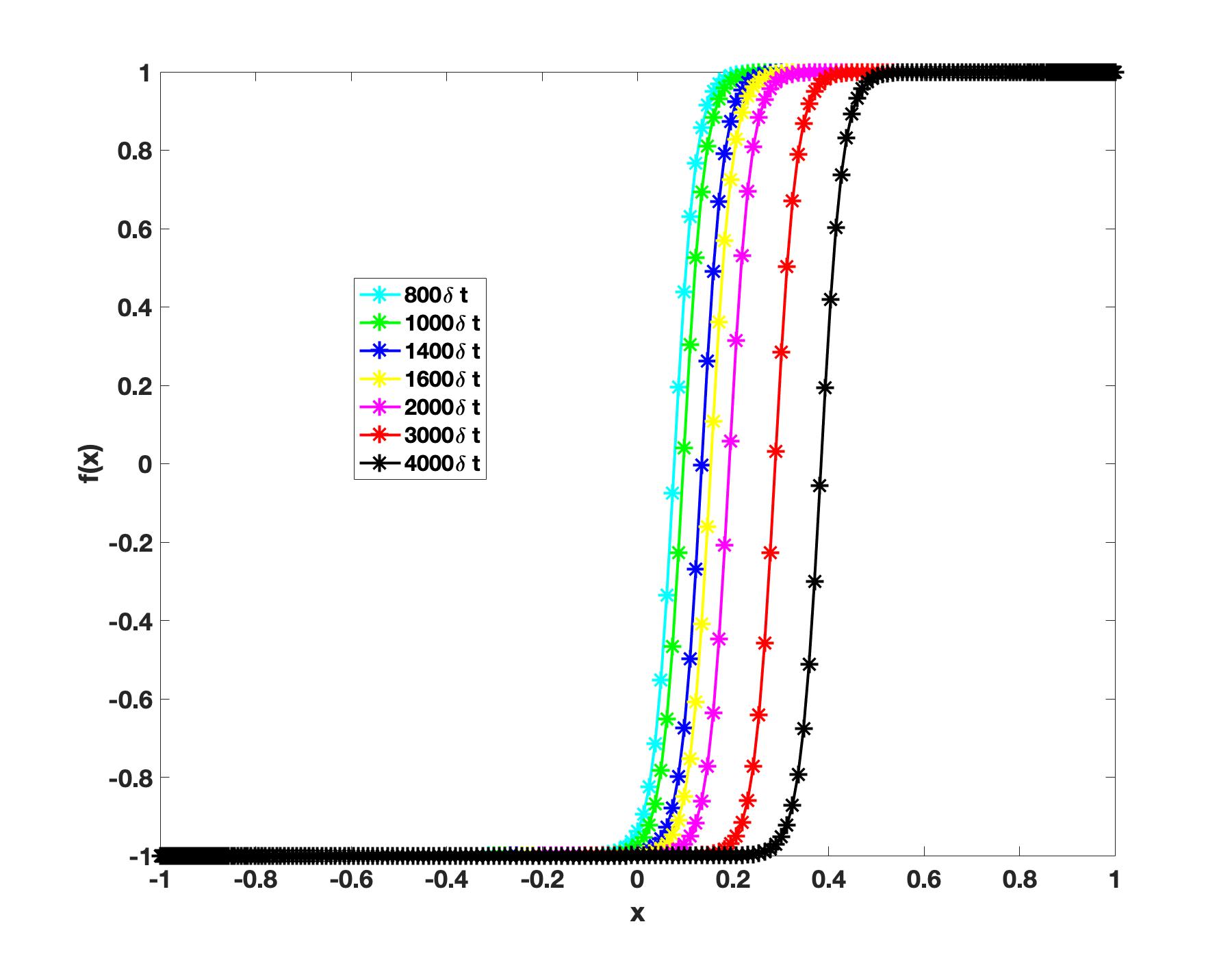
(d) Numerical method in Eulerian coordinate, $\epsilon^{2}=0.001$, $N=256$.

Figure 9. Approximate solutions for the generalized Allen-Cahn equation.

5.3. Two dimensional axis-symmetric case

As a final example, we examine the performance of our flow dynamic approach for a two dimensional axis-symmetric case with $\Omega=\{x^{2}+y^{2}<1\}$ and initial condition $f_{0}(x)=x$. More precisely, we solve (4.7) with $\epsilon^{2}=0.001$ using the Lagrangian scheme with a spectral method in space with $N=16,64$. Since (4.7) is axi-symmetric, we only plot the one-dimensional profiles in Fig. 10.

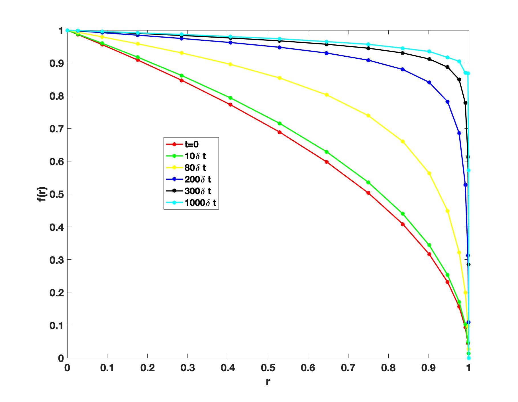
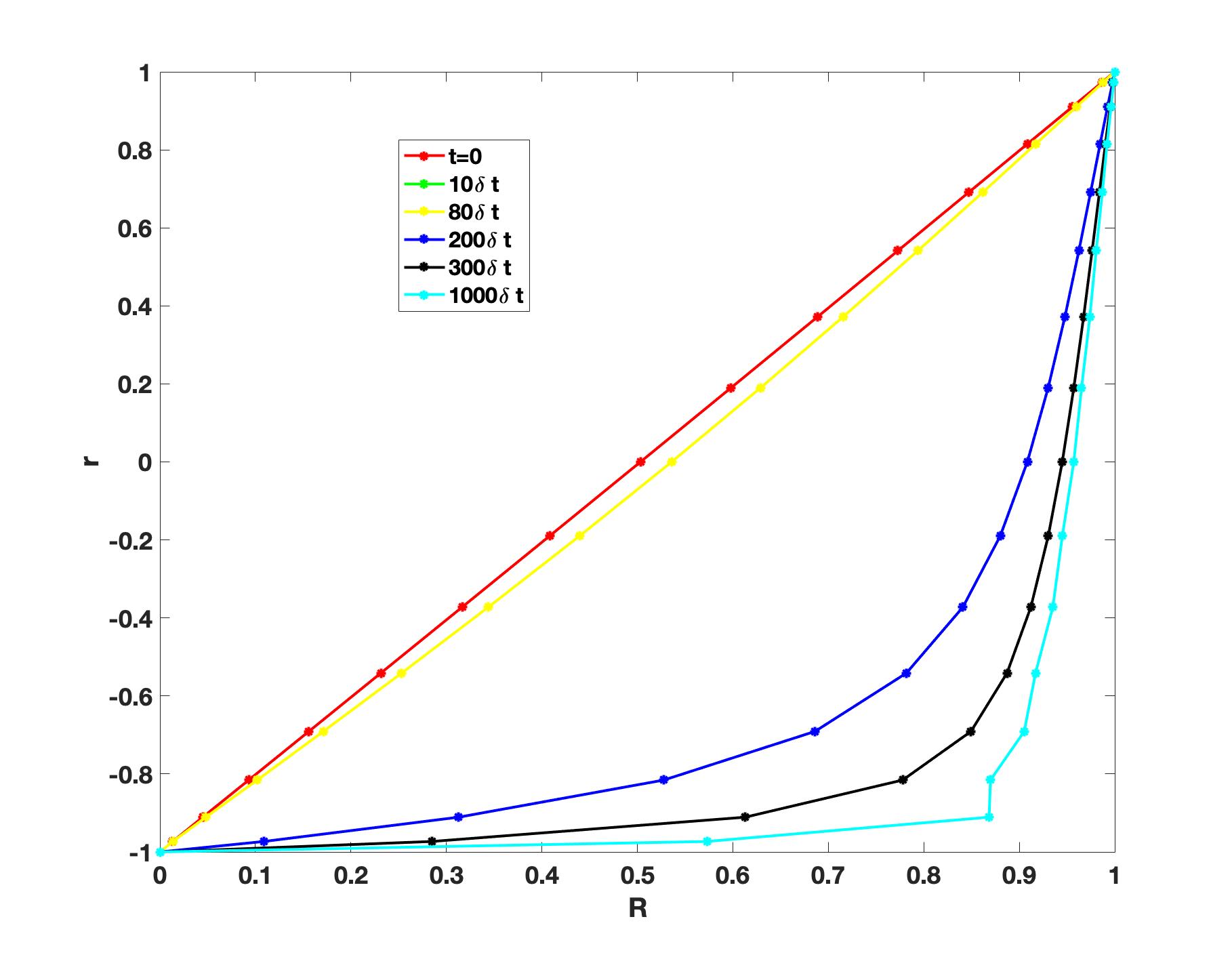
(a) Flow dynamic approach with spectral method of $N=16$.

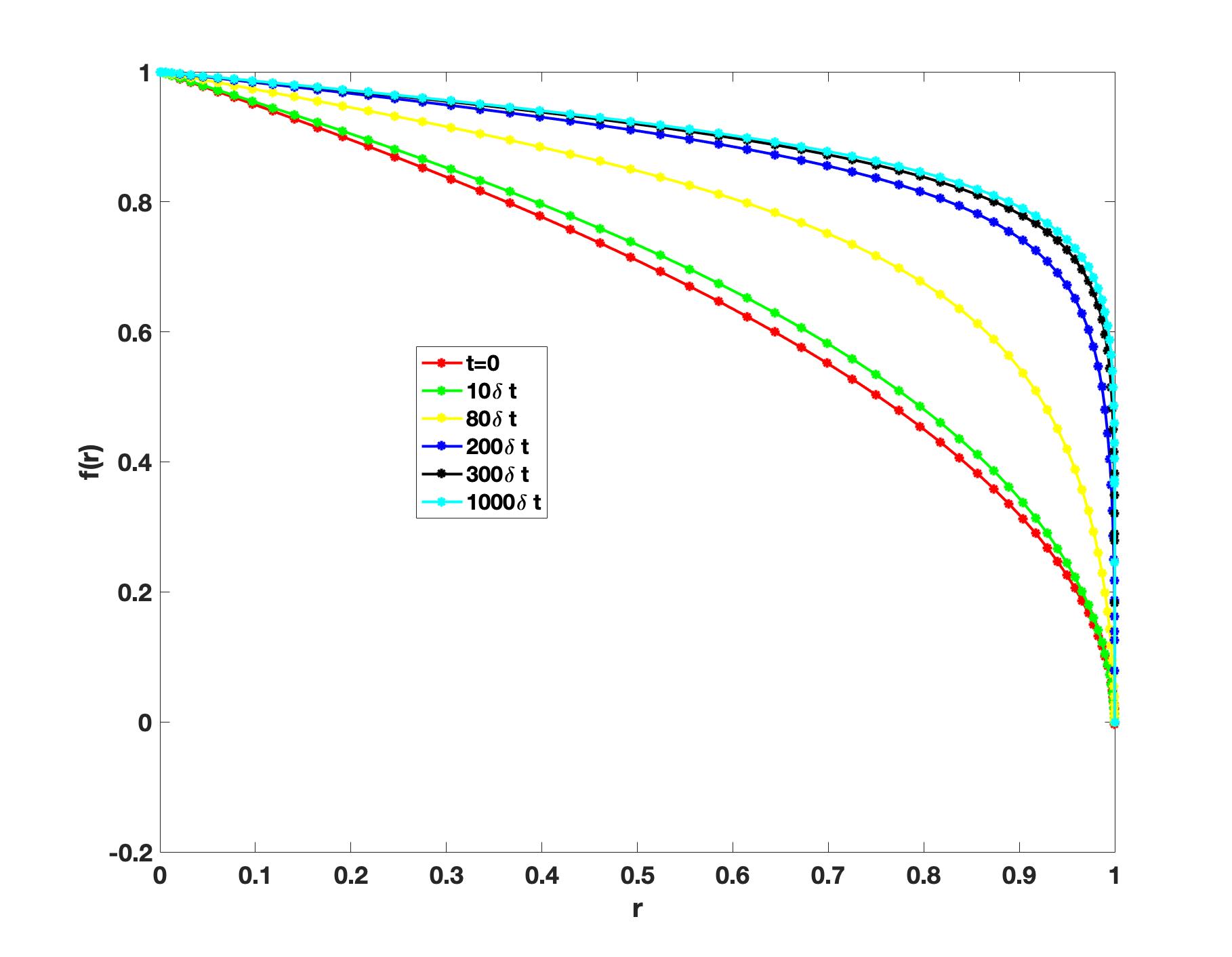
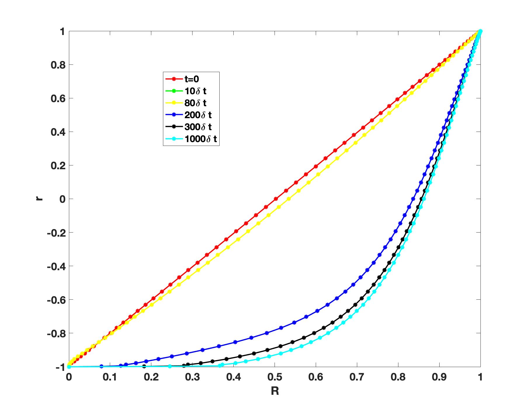
(b) Flow dynamic approach with spectral method of $N=64$.

Figure 10. Axis-symmetric case computed by Lagrangian numerical method with $\epsilon^{2}=0.001$ and time step $\delta t=10^{-4}$.

6. Concluding remarks

We presented in this paper a new Lagrangian approach which can effectively capture the thin interface of the Allen-Cahn type equations. Using the energetic variational approach, we introduced a transport equation and reformulated the Allen-Cahn equation in Eulerian coordinates to a trajectory equation for the flow map in Lagrangian coordinates. We then developed effective energy stable schemes for the highly nonlinear trajectory equation, and presented ample numerical results to show the effectiveness of this approach for interface capturing.

The main advantage of the new approach is that meshes, in the Eulerian coordinate through the flow map, automatically moves to the interfacial regions so that only a few points are needed to resolve thin interfaces. In fact, the number of points required to resolve interfacial layers of width $\epsilon$ is independent of $\epsilon$!

To fix the idea, we restricted ourselves to the one-dimensional case in this paper. In this case, the assumption that the flow velocity satisfies the transport equation (2.8) leads to a well-posed trajectory equation. But the transport equation (2.8) is not a suitable choice for multi-dimensional cases as it will lead to a trajectory equation which is not well-posed. However, the methodology introduced in this paper is still applicable for multi-dimensional cases and for other type of diffuse interface models such as Cahn-Hilliard models. The key is to use an alternative transport equation so that the resulting trajectory equation becomes well-posed. In a forthcoming paper, we shall apply the new Lagrangian approach introduced in this paper to multi-dimensional diffuse-interface models.

Appendix A Derivation by an energetic variational approach

We shall use the energetic variational approach to derive the Allen-Cahn equation (2.15) using flow map (LABEL:flow_map_AC) and kinematic relation (2.9).

A.1. Energy dissipative law with flow map

The energy dissipative law consisting the conservation function as well as the dissipation function plus kinematic relationship determine all the physical information for mathematical models. So we combine original energy dissipative law (2.3) with transport equation (2.9) together to define the singularity by using the Energetic Variational Approach. If we plug the kinematic equations (2.9) into the energy dissipative law (2.3), we can derive a equivalent energy dissipative law with respect to flow map of equation (LABEL:flow_map_AC) in Eulerian coordinate. For Allen-Cahn system (2.1)-(2.2), we have the new energy dissipative law as

(A.1) $$\left\{\begin{aligned} &\frac{d}{dt}\int_{\Omega_{\boldsymbol{x}}}\frac{1}{2}|\nabla_{\boldsymbol{x}}f|^{2}+\frac{1}{4\epsilon^{2}}(f^{2}-1)^{2}d\boldsymbol{x}=-\int_{\Omega_{\boldsymbol{x}}}|\boldsymbol{u}\cdot\nabla_{\boldsymbol{x}}f|^{2}d\boldsymbol{x},\\ &f_{t}+(\boldsymbol{u}\cdot\nabla_{\boldsymbol{x}})f=0.\end{aligned}\right.$$

Where the total free energy is $E^{total}:=\int_{\Omega_{\boldsymbol{x}}}w(f)d\boldsymbol{x}$ with free energy density $w:=\frac{1}{2}|\nabla_{\boldsymbol{x}}f|^{2}+\frac{1}{4\epsilon^{2}}(f^{2}-1)^{2}$, and ${\bf\Delta}$ is represented as

(A.2) $${\bf\Delta}=\int_{\Omega_{\boldsymbol{x}}}|\boldsymbol{u}\cdot\nabla_{\boldsymbol{x}}f|^{2}d\boldsymbol{x},$$

which is dissipative term with respect to velocity $\boldsymbol{u}$ and also can be regarded as entropy production from the Second Law of Thermodynamics. In order to derive the constitution equation of Allen-Cahn equation in terms of force balance, we need to introduce the framework of Least Action principle and Maximum Dissipative principle.

A.1.1. Least Action Principle

The Least Action Principle [1, 3] is interpreted as for a Hamiltonian system the trajectories of particles from position $\boldsymbol{x}(\boldsymbol{X},0)$ at time $t=0$ to position $\boldsymbol{x}(\boldsymbol{X},T)$ at time $t=T$ are determined by the variational of Least Action function with respect to trajectory flow map. From energy dissipative law (2.3), for Allen-Cahn equation, the least action function is defined as

(A.3) $$\begin{split}A(\boldsymbol{x}):&=-\int_{0}^{T}\mathcal{F}dt=-\int_{0}^{T}\int_{\Omega_{\boldsymbol{x}}}w(\nabla_{\boldsymbol{x}}f,f)d\boldsymbol{x}dt\\ &=-\int_{0}^{T}\int_{\Omega_{\boldsymbol{x}}}\frac{1}{2}|\nabla_{\boldsymbol{x}}f|^{2}+\frac{1}{4\epsilon^{2}}(f^{2}-1)^{2}d\boldsymbol{x}dt,\end{split}$$

where $\mathcal{F}$ is Helmholtz free energy and $w(\nabla_{\boldsymbol{x}}f,f)=\frac{1}{2}|\nabla_{\boldsymbol{x}}f|^{2}+\frac{1}{4\epsilon^{2}}(f^{2}-1)^{2}$. Since from the kinematic relationship defined by equation (2.9) in Allen-Cahn system, we have the following equalities in Lagrange coordinate

(A.4) $$f(\boldsymbol{x}(\boldsymbol{X},t),t):=f(\boldsymbol{X},0)=f_{0}(\boldsymbol{X}).$$

By (A.4), for Allen-Cahn system (2.1)-(2.2), using deformation tensor $F$, the action function is formulated as follows in Lagrangian coordinate

(A.5) $$A(\boldsymbol{x}):=-\int_{0}^{T}\int_{\Omega_{\boldsymbol{X}}}w(\nabla_{\boldsymbol{X}}f_{0}(\boldsymbol{X})(\frac{\partial\boldsymbol{x}}{\partial\boldsymbol{X}})^{-1},f_{0}(\boldsymbol{X}))detFdXdt.$$

Taking the variational derivative of action function $A(\boldsymbol{x})$ with respect to flow map $\boldsymbol{x}\rightarrow\boldsymbol{x}+\epsilon\boldsymbol{y}$ and combined with chain rule $\nabla_{\boldsymbol{x}}f=\nabla_{\boldsymbol{X}}f_{0}(\boldsymbol{X})(\frac{\partial\boldsymbol{x}}{\partial\boldsymbol{X}})^{-1}$, and notice the equality (A.4). Then we obtain

(A.6) $$\begin{split}\frac{\delta A}{\delta\boldsymbol{x}}&=\frac{d}{d\epsilon}|_{\epsilon=0}\int_{\Omega_{\boldsymbol{x}}}w(\nabla_{\boldsymbol{x}}f(\boldsymbol{x}+\epsilon\boldsymbol{y}),f(\boldsymbol{x}+\epsilon\boldsymbol{y}))d\boldsymbol{x}\\ &=\frac{d}{d\epsilon}|_{\epsilon=0}\int_{\Omega_{\boldsymbol{X}}}w(\nabla_{\boldsymbol{X}}f_{0}(\boldsymbol{X})(\frac{\partial(\boldsymbol{x}+\epsilon\boldsymbol{y})}{\partial\boldsymbol{X}})^{-1},f_{0}(\boldsymbol{X}))det(\frac{\partial(\boldsymbol{x}+\epsilon\boldsymbol{y})}{\partial\boldsymbol{X}})d\boldsymbol{X}\\ &=\int_{\Omega_{\boldsymbol{X}}}\frac{\partial w(\nabla_{\boldsymbol{x}}f,f)}{\partial\nabla_{\boldsymbol{x}}f}(-F^{-1}\frac{\partial\boldsymbol{y}}{\partial\boldsymbol{X}}F^{-1}\nabla_{\boldsymbol{X}}f_{0}(\boldsymbol{X}))detF+w(\nabla_{\boldsymbol{x}}f,f)detF\cdot tr(F^{-T}\frac{\partial\boldsymbol{y}}{\partial\boldsymbol{X}})d\boldsymbol{X}\\ &=\int_{\Omega_{\boldsymbol{X}}}-\frac{\partial w(\nabla_{\boldsymbol{x}}f,f)}{\partial\nabla_{\boldsymbol{x}}f}\otimes\nabla_{\boldsymbol{x}}f\frac{\partial\boldsymbol{y}}{\partial\boldsymbol{x}}+w(\nabla_{\boldsymbol{x}}f,f)\nabla_{\boldsymbol{x}}\cdot\boldsymbol{y}d\boldsymbol{x}\\ &=\int_{\Omega_{\boldsymbol{X}}}\nabla_{\boldsymbol{x}}\cdot(\frac{\partial w(\nabla_{\boldsymbol{x}}f,f)}{\partial\nabla_{\boldsymbol{x}}f}\otimes\nabla_{\boldsymbol{x}}f-w(\nabla_{\boldsymbol{x}}f,f)I)\boldsymbol{y}d\boldsymbol{x}=\int_{\Omega_{\boldsymbol{x}}}w_{f}\nabla_{\boldsymbol{x}}f\boldsymbol{y}d\boldsymbol{x}.\end{split}$$

Where $\frac{\delta w}{\delta f}=w_{f}=-\Delta_{\boldsymbol{x}}f+\frac{1}{\epsilon^{2}}f(f^{2}-1)$, $\frac{\delta w}{\delta f}$ is also called chemical potential and $I$ is identity matrix. According to Least Action Principle we have the conservative force as $F_{con}=\frac{\delta A}{\delta\boldsymbol{x}}$ in Eulerian coordinate.

As a consequence, we derive that

(A.7) $$F_{con}=\frac{\delta A}{\delta\boldsymbol{x}}=w_{f}\nabla_{\boldsymbol{x}}f.$$

In order to derive the constitution equation, as we have computed the conservative force (A.7) from the Least Action principle, the dissipative force shall be obtained from the following Maximum dissipative principle.

A.1.2. Maximum Dissipative Principle

The Maximum Dissipative Principle is also named as Onsager principle, .ie. the dissipative force can be obtain by taking variational of $\frac{1}{2}\bf\Delta$ with respect to velocity $\boldsymbol{u}$. Since $\bf\Delta$ is said to be quadratic in the rates, so the force is linear with respective rates.

(A.8) $$F_{dis}=\frac{\delta\frac{1}{2}\bf\Delta}{\delta\boldsymbol{u}}=\boldsymbol{u}\cdot\nabla_{\boldsymbol{x}}f\nabla_{\boldsymbol{x}}f.$$

A.2. Force balance and constitution equation

From Newton’s force balance law,

(A.9) $$F_{con}=F_{dis}$$

We derive the constitution equation of Allen-Cahn equation in Eulerian coordinate in combination of conservative force and dissipative force, for system (2.1)-(2.2)

(A.10) $$\begin{split}&w_{f}\nabla_{\boldsymbol{x}}f=\boldsymbol{u}\cdot\nabla_{\boldsymbol{x}}f\nabla_{\boldsymbol{x}}f,\\ &w_{f}=-\Delta_{\boldsymbol{x}}f+\frac{1}{\epsilon^{2}}f(f^{2}-1).\end{split}$$

Remark A.1.

For Allen-Cahn system (2.15), taking inner product of (2.15) with $-\boldsymbol{u}\cdot\nabla_{\boldsymbol{x}}f$ and notice the equality $f_{t}=-\boldsymbol{u}\cdot\nabla_{\boldsymbol{x}}f$. We can also derive the equivalent energy dissipative law (A.1) in Eulerian coordinate.

References

- [1] Ralph Abraham, Jerrold E Marsden, and Jerrold E Marsden. Foundations of mechanics, volume 36. Benjamin/Cummings Publishing Company Reading, Massachusetts, 1978.
- [2] Samuel M Allen and John W Cahn. A microscopic theory for antiphase boundary motion and its application to antiphase domain coarsening. Acta metallurgica, 27(6):1085–1095, 1979.
- [3] Vladimir Igorevich Arnol’d. Mathematical methods of classical mechanics, volume 60. Springer Science & Business Media, 2013.
- [4] Lia Bronsard and Robert V Kohn. Motion by mean curvature as the singular limit of ginzburg-landau dynamics. Journal of differential equations, 90(2):211–237, 1991.
- [5] Weiming Cao, Weizhang Huang, and Robert D Russell. A moving mesh method based on the geometric conservation law. SIAM Journal on Scientific Computing, 24(1):118–142, 2002.
- [6] Xinfu Chen, Danielle Hilhorst, and Elisabeth Logak. Mass conserving allen–cahn equation and volume preserving mean curvature flow. Interfaces and Free Boundaries, 12(4):527–549, 2011.
- [7] Sybren Ruurds De Groot and Peter Mazur. Non-equilibrium thermodynamics. Courier Corporation, 2013.
- [8] Q. Du, C. Liu, and X. Wang. A phase field approach in the numerical study of the elastic bending energy for vesicle membranes. J. Comput. Phys., 198:450–468, 2004.
- [9] Q. Du, C. Liu, and X. Wang. Simulating the deformation of vesicle membranes under elastic bending energy in three dimensions. J. Comput. Phys., 212:757–777, 2005.
- [10] Qiang Du and Xiaobing Feng. The phase field method for geometric moving interfaces and their numerical approximations. arXiv preprint arXiv:1902.04924, 2019.
- [11] Bob Eisenberg, Yunkyong Hyon, and Chun Liu. Energy variational analysis of ions in water and channels: Field theory for primitive models of complex ionic fluids. The Journal of Chemical Physics, 133(10):104104, 2010.
- [12] Lawrence C Evans, H Mete Soner, and Panagiotis E Souganidis. Phase transitions and generalized motion by mean curvature. Communications on Pure and Applied Mathematics, 45(9):1097–1123, 1992.
- [13] WM Feng, Peng Yu, SY Hu, Zi-Kui Liu, Qiang Du, and Long-Qing Chen. Spectral implementation of an adaptive moving mesh method for phase-field equations. Journal of Computational Physics, 220(1):498–510, 2006.
- [14] Xiaobing Feng and Andreas Prohl. Analysis of a fully discrete finite element method for the phase field model and approximation of its sharp interface limits. Mathematics of computation, 73(246):541–567, 2004.
- [15] Mi-Ho Giga, Arkadz Kirshtein, and Chun Liu. Variational modeling and complex fluids. Handbook of mathematical analysis in mechanics of viscous fluids, pages 1–41, 2017.
- [16] Andreas Greven, Gerhard Keller, and Gerald Warnecke. Entropy, volume 47. Princeton University Press, 2014.
- [17] Morton E Gurtin, Eliot Fried, and Lallit Anand. The mechanics and thermodynamics of continua. Cambridge University Press, 2010.
- [18] Jan Hesthaven and Robert Kirby. Filtering in legendre spectral methods. Mathematics of Computation, 77(263):1425–1452, 2008.
- [19] Weizhang Huang, Yuhe Ren, and Robert D Russell. Moving mesh methods based on moving mesh partial differential equations. Journal of Computational Physics, 113(2):279–290, 1994.
- [20] Tom Ilmanen et al. Convergence of the allen-cahn equation to brakke???s motion by mean curvature. J. Differential Geom, 38(2):417–461, 1993.
- [21] Markos Katsoulakis, Georgios T Kossioris, and Fernando Reitich. Generalized motion by mean curvature with neumann conditions and the allen-cahn model for phase transitions. The Journal of Geometric Analysis, 5(2):255, 1995.
- [22] Frank M Leslie. Theory of flow phenomena in liquid crystals. In Advances in liquid crystals, volume 4, pages 1–81. Elsevier, 1979.
- [23] Bo Li and Jian-Guo Liu. Thin film epitaxy with or without slope selection. European Journal of Applied Mathematics, 14(06):713–743, 2003.
- [24] Ruo Li, Tao Tang, and Pingwen Zhang. Moving mesh methods in multiple dimensions based on harmonic maps. Journal of Computational Physics, 170(2):562–588, 2001.
- [25] Chun Liu and Jie Shen. A phase field model for the mixture of two incompressible fluids and its approximation by a fourier-spectral method. Physica D: Nonlinear Phenomena, 179(3-4):211–228, 2003.
- [26] JA Mackenzie and ML Robertson. A moving mesh method for the solution of the one-dimensional phase-field equations. Journal of Computational Physics, 181(2):526–544, 2002.
- [27] Yurii Nesterov and Arkadii Nemirovskii. Interior-point polynomial algorithms in convex programming, volume 13. Siam, 1994.
- [28] Lars Onsager. Reciprocal relations in irreversible processes. i. Physical review, 37(4):405, 1931.
- [29] Lars Onsager. Reciprocal relations in irreversible processes. ii. Physical review, 38(12):2265, 1931.
- [30] J. Shen. Efficient spectral-Galerkin method I. direct solvers for second- and fourth-order equations by using Legendre polynomials. SIAM J. Sci. Comput., 15:1489–1505, 1994.
- [31] Jie Shen and Xiaofeng Yang. An efficient moving mesh spectral method for the phase-field model of two-phase flows. Journal of computational physics, 228(8):2978–2992, 2009.
- [32] Jie Shen and Xiaofeng Yang. Numerical approximations of Allen-Cahn and Cahn-Hilliard equations. Discrete Contin. Dyn. Syst, 28(4):1669–1691, 2010.
- [33] Hervé Vandeven. Family of spectral filters for discontinuous problems. Journal of Scientific Computing, 6(2):159–192, 1991.
- [34] Juan Luis Vázquez. The porous medium equation: mathematical theory. Oxford University Press, 2007.
- [35] Shixin Xu, Ping Sheng, and Chun Liu. An energetic variational approach for ion transport. arXiv preprint arXiv:1408.4114, 2014.
- [36] Jian Zhang and Qiang Du. Numerical studies of discrete approximations to the allen–cahn equation in the sharp interface limit. SIAM Journal on Scientific Computing, 31(4):3042–3063, 2009.