Quantum Darwinism and Non-Markovianity in a Model of Quantum Harmonic Oscillators

Abstract

To explain aspects of the quantum-to-classical transition, quantum Darwinism explores the fact that, due to interactions between a quantum open system and its surrounding environment, information about the system can be spread redundantly to the environment. Here we recall that there are in the literature two distinct and non-equivalent ways to make this statement precise and quantitative. We first point out the difference with some simple but illustrative examples. We then consider a model where Darwinism can be seen from both perspectives. Moreover, the non-Markovianity of our model can be varied with a parameter. In a recent work [F. Galve et al., Sci. Reps. 6, 19607 (2016)], the authors concluded that quantum Darwinism can be hindered by non-Markovianity. We depart from their analysis and argue that, from both perspectives to quantum Darwinism, there is no clear relationship between non-Markovianity and quantum Darwinism in our model.

I Introduction

Since the formulation of quantum theory, problems with the quantum-to-classical transition have been highlighted, for instance, by the Schrödinger’s cat gedanken experiment schcat and the EPR “paradox” epr . In particular, the superposition principle and the quantum state “fragility” under measurements are, at a first glance, difficult to conflate with basic notions of classical physics. However, considerable progress was made in the past decades by taking into account that effectively classical systems, besides being macroscopic, are typically open zur1981 ; zur2003 ; schl2007 .

The fact that macroscopic systems are never seen in superposition states with distinct macroscopic properties is essentially explained by the effect of decoherence zur2003 ; zur1982 ; bru1996 ; dav1996 ; bre2002 ; zur2005a ; schl2007 . Indeed, every physical system constantly interacts with its surrounding environment. For macroscopic systems this interaction can never be completely neglected (except, perhaps, under extremely artificial laboratory conditions). In fact, it implies that any coherence between macroscopically distinct states will quickly vanish, transforming superpositions of such states into statistical mixtures.

Openness is also an important ingredient to explain why macroscopic systems, when in their naturally realized states, are essentially insensitive to measurements. In Refs. zur2004 ; zur2003a ; zur2005 ; zur2006 ; zur2005b ; zunatk2009 the authors observed that the environment can monitor a so-called preferred observable of the system and store information about it. This is done in such a way that it is possible to extract information about it indirectly and disturbing the system minimally (beyond what it was already disturbed by the environment). More than that, different regions of the environment record that information redundantly, so it is sufficient to access just a small fragment to obtain a significant amount of information about the preferred observable of the macroscopic system. This is roughly the idea behind quantum Darwinism.

The concept of quantum Darwinism has been explored in several models, like in spin systems zur2009 , where the environment monitors the spin of a particle; in a quantum Brownian particle zur2008 , where the environment monitors its position; and recently in an experimental work, within a nitrogen vacancy center zur2018 . Moreover, the role of Markovianity in the emergence of quantum Darwinism was studied recently in Refs. mas2019 and sab2016 . In Ref. sab2016 the authors discuss a relationship between quantum Darwinism and non-Markovianity concluding that non-Markovianity can hinder quantum Darwinism.

As originally proposed (see, for instance, Ref. zur2003 ), from the global system-environment state at some instant of time, one can compute the quantum mutual information between the system and fractions of the environment. That can be used to measure both the amount and redundancy of information about the system state that is available in the environment at that instant of time, regardless of the initial state of both system and environment. Alternatively, one can look at how initial states of the system are mapped to states in fractions of the environment after some interaction time bra2015 ; hor2015 . From that, one can check if some information about a system observable before the interaction can be recovered from measurements in these environment fractions after the interaction.

In this paper we address the differences in these two approaches, first, through simple examples. We then investigate them in a model of a quantum harmonic oscillator coupled to an environment also composed of quantum harmonic oscillators. Furthermore, we can range the dynamics of the main oscillator from Markovian to non-Markovian by tuning one of the parameters of the model. This allows us to explore carefully the relationship between non-Markovianity and quantum Darwinism. Following the definition given in sab2016 to estimate the “degree of quantum Darwinism”, we get results qualitatively similar to theirs, in the sense that it suggests that “non-Markovianity hinders quantum Darwinism”. However, we argue that we should estimate quantum Darwinism from other points of views. From these, we actually do not see any clear relationship between the two concepts.

In Sec. II we recall the ideas behind two approaches to quantum Darwinism and, in Sec. III, some basic notions of non-Markovianity. We define the model in Sec. IV and discuss its relevant properties. In Sec. V and VI we discuss quantum Darwinism in our model from these two aforementioned perspectives. In Sec. VII we discuss the relationship (or absence of it) between quantum Darwinism and non-Markovianity. Finally, we close our paper with some concluding remarks in Sec. VIII.

II Quantum Darwinism(s)

Whenever a system $S$ and its environment $E$ interact with each other, information about the system can be transferred to the environment and, in some cases, the environment behaves, effectively, as a measurement apparatus zur1982 ; zur2003 . Typically, and especially for macroscopic systems, superposition states among elements in some special basis are rapidly “destroyed” and they lose coherence. This process is called decoherence bre2002 and that basis is referred to as the preferred basis (or observable) of the system.

The main idea of quantum Darwinism is that one additionally should take into account that the environment is composed of several subsystems. One can consider then distinct fragments composed by a subset of these subsystems. These fragments can record information redundantly about the macroscopic system in such a way that just a small piece of the environment is enough to obtain nearly all information available in the whole environment about the preferred observable of the system.

For a given model in which Darwinism is expected to take place, it is important to identify the system observable that the environment monitors. For instance, in the model studied in Ref. zur2008 , the preferred observable is the position of a quantum harmonic oscillator, while in the model studied in Ref. zur2009 the observable monitored is the $z$ component of a spin-$1/2$ system.

The monitored observable is easily recognized when, for some orthonormal basis $\{{|{\phi^{i}}\rangle}\}$ in the system Hilbert space and an environment initial state ${|{\Psi}\rangle}$, the global dynamics is

$$(\sum_{i}\alpha_{i}{|{\phi^{i}}\rangle})\otimes{|{\Psi}\rangle}\mapsto\sum_{i}\alpha_{i}{|{\phi^{i}}\rangle}\otimes{|{\Psi^{i}}\rangle},$$ (1)

where $\alpha_{i}$ are the complex coefficients of the system initial state and ${|{\Psi^{i}}\rangle}$ are environment states after the interaction with the system. If the states ${|{\Psi^{i}}\rangle}$ are mutually orthogonal, a global measurement on the environment, in a basis including the vectors ${|{\Psi^{i}}\rangle}$, is equivalent to a measurement on the system in the basis $\{{|{\phi^{i}}\rangle}\}$, making the former the preferred basis. Note that, in this case, evolution Eq. (1) is exactly the premeasurement of the von Neumann measurement scheme von2018mathematical . In the Darwinist regime, however, already local measurements on small portions of the environment should be enough. An extreme case would be the one where ${|{\Psi^{i}}\rangle}=\otimes_{k=1}^{N}{|{\psi_{k}^{i}}\rangle}$, if the environment has $N$ individual subsystems, with $\{{|{\psi_{k}^{i}}\rangle}\}$ being mutually orthogonal states of an individual environment subsystem $k$. Indeed, a measurement on environment subsystem $k$, in a basis which includes the vectors ${|{\psi_{k}^{i}}\rangle}$, is already equivalent to a measurement on the system in the basis $\{{|{\phi^{i}}\rangle}\}$.

For a general dynamics, or for general states, one needs a proper framework to address the problem. In the next section, we discuss the two main approaches available in the literature.

II.1 The Partial Information Plot approach

As initially proposed by Blume-Kohout and Zurek, the quantum mutual information can be used to quantify the redundancy of information about the system that is available in the environment, through the so-called partial information plot (PIP) zur2005 . Assume a quantum system $S$ and an environment $E$ composed of $N$ individual quantum systems. If the global state is $\rho$, for a certain environment fragment $F\subset E$ (that is, any subset of quantum systems from the environment), the mutual information between $S$ and $F$ is

$$I(S:F)=H(S)+H(F)-H(SF),\noindent$$ (2)

where $H(S)$, $H(F)$ and $H(SF)$ are the von-Neumann entropies of $S$, $F$ and $S+F$, respectively, with $H(X)=-\text{Tr}[\rho_{X}\ln{\rho_{X}}]$ for the reduced state $\rho_{X}$ of subsystem $X$. The idea is to compute $\bar{I}(f)$, defined by the average of $I(S:F)$ over all possible environment fragments $F$ composed by $fN$ individual subsystems, where $0\leq f\leq 1$ is the fraction of the environment that is taken. For pure global states, this curve is always antisymmetric with respect to the coordinate system defined by $\bar{I}=H(S)$ and $f=0.5$ zur2005 (see Fig. 1). Moreover, $H(S)$ should be the maximum amount of information that can be retrieved about the preferred observable (see Sec. II.3 for an example). Therefore, in the Darwinistic regime, $\bar{I}(f)$ should be close to $H(S)$ already for small $f$, and the PIP should look like a plateau (see the solid line in Fig. 1), since that implies that almost all information about the preferred observable is already available in small fractions of the environment.

Considering the above, it is useful to define, for arbitrary $0<\delta<1$, the smallest fragment size $f_{\delta}$ such that $\bar{I}(f_{\delta})>(1-\delta)H(S)$. The quantity

$$R_{\delta}=\frac{1}{f_{\delta}}\noindent$$ (3)

measures then the redundancy in the information about the preferred observable of the system. Indeed, the closer the PIP is to a plateau, the smaller is $f_{\delta}$ for a fixed value of $\delta$ and, hence, the larger $R_{\delta}$ is (see Fig. 1).

Figure 1: Three qualitatively distinct possibilities for a partial information plot (PIP). The solid line $(a)$ corresponds to a case where a small fraction of the environment already has average mutual information close to $H(S)$, being the signature of quantum Darwinism. The linear profile $(b)$ can be seen (approximately) in our model for small interaction times (see Sec. V). In profile $(c)$, $f_{\delta}$ is close to $0.5$, so the redundancy is very small. This kind of profile can be obtained from random pure states drawn according to the Haar measure zur2005 .

II.2 The BPH approach

An alternative idea is to look at how initial states of the system are mapped into states of the environment, as proposed in Ref. bra2015 by F. Brandão et. al., which we call the BPH approach for short (see also a related approach in hor2015 ). There, they take as the fundamental object a completely positive map $\Lambda_{E}:D_{S}\rightarrow D_{E}$, where $D_{S}$ and $D_{E}$ are the state spaces of the system and environment, respectively. Physically, this map is the result of partial tracing the system after system and environment evolved for some fixed amount of time and a fixed initial environment state (see Sec. II.3 for an example). Since the environment is composed of many subsystems, one can define, via composition with partial tracing, corresponding maps $\Lambda_{F}:D_{S}\rightarrow D_{F}$ to each fragment $F$ of the environment, namely,

$$\Lambda_{F}=\text{Tr}_{E-F}\circ\Lambda_{E}.$$

A preferred observable would be in general described by a positive operator valued measure (POVM) $\{M_{i}\}$ and distinguished by the condition:

$$\Lambda_{F}(\rho)\approx\sum_{i}\text{Tr}(M_{i}\rho)\sigma_{i,F}$$

for every system operator $\rho$ and some states $\sigma_{i,F}$ for environment fraction $F$. The approximation must hold for most environment fractions $F$ and the POVM $\{M_{i}\}$ must be independent of $F$. The expression on the right-hand side is a so-called measure and prepare map. If states $\sigma_{i,F}$ are sufficiently distinguishable (for distinct values of $i$), some measurement can be done on $F$ to infer the statistics of the preferred observable on the state $\rho$, that is, the set of values $\{\text{Tr}(M_{i}\rho)\}$.

They further formulate the concepts of emergent objectivity of the observables and outcomes and show their validity under some circumstances bra2015 ; kno2018 . The objectivity of observables guarantees that all observers have access to the same observable (namely, $\{M_{i}\}$ is independent of $F$), and it is a generic feature of quantum mechanics bra2015 . The objectivity of outcomes occurs when different observers, who access different fragments of the environment, agree with the results of their measurements. It is guaranteed to take place when the outcomes of measurement on these fragments contain almost all information about the preferred observable (roughly speaking, for almost all $F$, the states $\sigma_{F,i}$ must be highly distinguishable for distinct values of $i$).

II.3 Examples

We discuss here two simple examples with a two-fold objective: to highlight the ideas behind both perspectives of quantum Darwinism, making explicit their non-equivalence, and to serve as toy models to two distinct time regimes of the model we shall discuss in Sec. IV.

Example 1. Assume the main system $S$ is a qubit and the environment $E$ is composed of $N$ qubits, for which we use the set of labels $E=\{1,...,N\}$. Assume further that the environment initial state is ${|{0}\rangle}_{E}:=\otimes_{k\in E}{|{0}\rangle}_{k}$ and their joint dynamics, after some fixed time interval $T$, is given by

$${|{0}\rangle}{|{0_{E}}\rangle}\mapsto{|{0}\rangle}{|{0_{E}}\rangle},$$ (4)

$${|{1}\rangle}{|{0_{E}}\rangle}\mapsto{|{1}\rangle}{|{1_{E}}\rangle},$$ (5)

where ${|{1_{E}}\rangle}:=\otimes_{k\in E}{|{1}\rangle}_{k}$. Therefore, if the initial state of the system is $\frac{1}{\sqrt{2}}({|{0}\rangle}+{|{1}\rangle})$, the evolved state is the GHZ state

$$\frac{1}{\sqrt{2}}({|{0}\rangle}{|{0_{E}}\rangle}+{|{1}\rangle}{|{1_{E}}\rangle}).$$ (6)

For any proper fragment $F\subset{E}$ of the environment, it holds:

$$\rho_{SF}=\frac{1}{2}{|{0}\rangle}\!{\langle{0}|}{|{0_{F}}\rangle}\!{\langle{0_{F}}|}+\frac{1}{2}{|{1}\rangle}\!{\langle{1}|}{|{1_{F}}\rangle}\!{\langle{1_{F}}|},$$

where ${|{0_{F}}\rangle}=\otimes_{k\in F}{|{0}\rangle}_{k}$ and analogously for ${|{1_{F}}\rangle}$. Therefore, by measuring the environment fraction $F$ in the basis $\{{|{0_{F}}\rangle},{|{1_{F}}\rangle}\}$, one can predict with a certainty the outcome of a $\{{|{0}\rangle},{|{1}\rangle}\}$ measurement in $S$, at time $T$. On the other hand, no measurement whatsoever in $F$ will reveal any information about, say, a $\{{|{+}\rangle},{|{-}\rangle}\}$ measurement in $S$, where ${|{\pm}\rangle}=\frac{1}{\sqrt{2}}({|{0}\rangle}\pm{|{1}\rangle})$. Indeed, it is easy to check that for both outcomes of such a measurement in the system, the corresponding states, for a proper environment fragment, are identical. Therefore, no measurement in a proper fragment would be able to distinguish these two states and there would be no way to predict (better than a random guess) the measurement outcome of the system. This reinforces the fact that $\{{|{0}\rangle},{|{1}\rangle}\}$ is the preferred basis (or observable).

However, the global state can also be written as

$$\frac{1}{\sqrt{2}}({|{+}\rangle}{|{\text{GHZ}_{+}}\rangle}+{|{-}\rangle}{|{\text{GHZ}_{-}}\rangle}),$$

where ${|{\text{GHZ}_{\pm}}\rangle}=\frac{1}{\sqrt{2}}({|{0_{E}}\rangle}\pm{|{1_{E}}\rangle}).$ Therefore, if one has access to the whole environment, a measurement in the basis $\{{|{\text{GHZ}_{+}}\rangle},{|{\text{GHZ}_{-}}\rangle}\}$ actually allows one to infer the outcome of a $\{{|{+}\rangle},{|{-}\rangle}\}$ measurement in $S$. Note that, moreover, the same is true for any system observable, defined by an arbitrary orthonormal basis.

It is easy to check that the PIP for state Eq. (6) is an exact plateau: $\bar{\mathcal{I}}(0)=0$ by definition, $\bar{\mathcal{I}}(f)=H(S)=\ln{2}$ for every $0<f<1$ and $\bar{\mathcal{I}}(f)=2H(S)=2\ln{2}$ for $f=1$. This reflects the fact that any proper subset of the environment only has information about the preferred observable. The environment as a whole, on the other hand, has potential information about any observable of the system. But, of course, to predict with certainty the outcomes of other observables, a global measurement in the whole environment must be done (such as a measurement in the basis $\{{|{\text{GHZ}_{+}}\rangle},{|{\text{GHZ}_{-}}\rangle}\}$), so there is no redundancy whatsoever.

This example can be also understood from the BPH perspective. Here we have, for any environment fragment $F\subset E$,

$$\Lambda_{F}(\rho)=\text{Tr}({|{0}\rangle}\!{\langle{0}|}\rho){|{0_{F}}\rangle}\!{\langle{0_{F}}|}+\text{Tr}({|{1}\rangle}\!{\langle{1}|}\rho){|{1_{F}}\rangle}\!{\langle{1_{F}}|}.$$ (7)

That is, the maps are exactly measure and prepare maps, with POVM $\{{|{0}\rangle}\!{\langle{0}|},{|{1}\rangle}\!{\langle{1}|}\}$, and the corresponding environment states are perfectly distinguishable. Therefore, we can think that the environment acquires redundant information about the preferred observable on the initial state of the system. More specifically, a $\{{|{0_{F}}\rangle},{|{1_{F}}\rangle}\}$ measurement on the environment has exactly the same statistics of a $\{{|{0}\rangle},{|{1}\rangle}\}$ measurement on $S$ for every system state $\rho$. Moreover, one has complete objectivity of outcomes. If observers measure environment qubits in the basis $\{{|{0}\rangle},{|{1}\rangle}\}$, they will always agree on the outcome. For instance, if some of them observes outcome $0$, all of them will also observe that same outcome.

Note that in the PIP approach, since one considers only the specific global state Eq. (6), a strong claim can be made: If someone observes a certain outcome upon a $\{{|{0}\rangle},{|{1}\rangle}\}$ measurement in an environment fragment $F$, we can be certain that a $\{{|{0}\rangle},{|{1}\rangle}\}$ measurement in the system itself, if performed, will show the same outcome. In the BPH there is no analog claim. It is not correct to say in general that, upon seeing the outcome $0$ in an environment $F$, the system was in state ${|{0}\rangle}$ at $T=0$, since the system could have been, say, in the initial state $\frac{1}{\sqrt{2}}({|{0}\rangle}+{|{1}\rangle})$ and there would be still a positive probability for observing the outcome $0$ in the environment fractions.

It is interesting to note that, from this perspective, in contrast to the PIP approach, having access to the whole environment does not have any additional consequence. One still is restricted to obtain information about the preferred observable .

Example 2. Now, consider a slight modification in the dynamics:

$${|{0}\rangle}{|{0_{E}}\rangle}\mapsto{|{0}\rangle}{|{0_{E}}\rangle},$$ (8)

$${|{1}\rangle}{|{0_{E}}\rangle}\mapsto{|{0}\rangle}{|{1_{E}}\rangle}.$$ (9)

No matter what initial state we choose for system $S$, it will never correlate with the environment, so the PIP is always trivial. From this perspective then, it appears that this is a bad instance of quantum Darwinism.

From the BPH perspective, however, they are essentially the same. Indeed, the maps $\Lambda_{F}$ defined by this dynamics are exactly the same as in Eq. (7) for every proper subset $F\subset E$. Nevertheless, as a side note, it is interesting to see that they do differ for $F=E$. In this case, having access to the whole environment does have a consequence. Indeed, the dynamics essentially transfer any initial state of the system to the environment:

$$(\alpha{|{0}\rangle}+\beta{|{1}\rangle}){|{0_{E}}\rangle}\mapsto{|{0}\rangle}(\alpha{|{0_{E}}\rangle}+\beta{|{1_{E}}\rangle}).$$ (10)

Therefore, one can choose to obtain information about an arbitrary system observable, in the sense that there exists some (in general, global) measurement that can be done in the whole environment that will have the exact same statistics of the corresponding system observable in the initial system state. Of course, these measurements being global makes meaningless the notion of objectivity, since it would not be possible to compare the outcomes of different observers.

III Non-Markovianity

A quantum dynamical system whose quantum maps $\Lambda_{t,t^{\prime}}$ are divisible in other completely positive maps, i.e., $\Lambda_{t_{2},t_{0}}=\Lambda_{t_{2},t_{1}}\Lambda_{t_{1},t_{0}}$ for all $t_{0}\leq t_{1}\leq t_{2}$, is said to be Markovian. Otherwise, the evolution is classified as non-Markovian wol2008 ; riv2014 . There are several different ways to quantify non-Markovianity riv2014 ; nad2015 ; nad2017 , and in this paper we estimate the non-Markovianity degree through the time variation of the distance between two random initial states lac2015 .

It is known that in a Markovian system, the distinguishability between any two states never increases and the flow of information has just one direction: from the system to the environment. Yet, in a non-Markovian dynamics this is not guaranteed. As they evolve, they can become more distinguishable and the information received by the environment can go back to the system sab2011 ; sab2017 .

One possible way to measure the distance between two states $\rho_{1}$ and $\rho_{2}$ is by the fidelity,

$$\mathcal{F}(\rho_{1},\rho_{2})=\text{Tr}\sqrt{\sqrt{\rho_{1}}\rho_{2}\sqrt{\rho_{1}}},\noindent$$ (11)

which behaves monotonically under the action of any quantum map. Then, we can define the non-Markovianity degree as

$$\mathcal{N}=\underset{\rho_{1},\rho_{2}}{\text{max}}\left[-\int_{\dot{\mathcal{F}}<0}\dot{\mathcal{F}}(\rho_{1},\rho_{2})dt\right],\noindent$$ (12)

where the maximization is over all possible pairs of initial states and $\dot{\mathcal{F}}$ is the time derivative bre2009 .

IV The Model

We now consider a model of a main quantum harmonic oscillator coupled to an environment of several quantum harmonic oscillators. The Hamiltonian, for $N$ environment oscillators, is defined by

$$H=\hbar\omega_{0}a^{\dagger}a+\hbar\sum_{k=1}^{N}\omega_{k}b_{k}^{\dagger}b_{k}+\hbar\sum_{k=1}^{N}\gamma_{k}(a^{\dagger}b_{k}+ab_{k}^{\dagger})\noindent,$$ (13)

where $\omega_{0}$ is the main oscillator frequency, $\omega_{k}$ is the $k$-th environment oscillator frequency, $a$, $a^{\dagger}$, $b_{k}$, and $b_{k}^{\dagger}$ are the creation and annihilation operators of the main system and the $k$-th environment oscillator, and $\gamma_{k}$ are coupling constants for the interaction between the $k$-th environment oscillator and the main oscillator. We shall set from now on $\hbar=1$.

Such model can be used to describe dissipation in optical cavities scu1997 , the dynamical properties of multipartite entanglement bet2014 and principles of quantum thermodynamics rap2018 . Here we show that it also offers a good benchmark to study quantum Darwinism and its connection with Markovianity.

Assume that initially the environment is in the vacuum state and the main oscillator is in a coherent state with parameter $\alpha_{0}\in\mathbb{C}$, that is,

$${|{\alpha_{0}}\rangle}\otimes\prod_{k=1}^{N}{|{0_{k}}\rangle}.$$ (14)

The global state evolution can be obtained exactly by the ansatz scu1997

$${|{\alpha(t)}\rangle}\otimes\prod_{k=1}^{N}{|{\lambda_{k}(t)}\rangle},\noindent$$ (15)

where ${|{\alpha(t)}\rangle}$ and ${|{\lambda_{k}(t)}\rangle}$ denote coherent states of the main oscillator and of the $k$-th environment oscillator, respectively. Schrödinger’s equation with the Hamiltonian Eq. (13) is satisfied as long as the coherent states parameters $\alpha(t)$ and $\lambda_{k}(t)$ satisfy

$$i\dot{\alpha}(t) = \omega_{0}\alpha(t)+\sum_{k}\gamma_{k}\lambda_{k}(t),$$ (16)

$$i\dot{\lambda}_{k} = \omega_{k}\lambda_{k}+\gamma_{k}\alpha(t).\noindent$$ (17)

We will consider the initial state of the main oscillator in superpositions of coherent states and the environment in the vacuum state,

$${|{\Psi(0)}\rangle}=G\left[\left(a{|{\alpha_{0}}\rangle}+b{|{-\alpha_{0}}\rangle}\right)\otimes\prod_{k=1}^{N}{|{0_{k}}\rangle}\right]\noindent,$$ (18)

where ${|{\pm\alpha_{0}}\rangle}$ are coherent states with parameters $\pm\alpha_{0}$, $a$ and $b$ are complex coefficients, and the normalization factor is given by $G=(|a|^{2}+|b|^{2}+ab^{*}\braket{-\alpha_{0}}{\alpha_{0}}+\text{c.c.})^{-1/2}$.

From the linearity of Schrodinger’s equation, the state of the composed system for any time $t$ is

$${|{\Psi(t)}\rangle}=G\left(a{|{\alpha(t)}\rangle}\otimes{|{\Lambda(t)}\rangle}+b{|{-\alpha(t)}\rangle}\otimes{|{-\Lambda(t)}\rangle}\right)\noindent,$$ (19)

where

$${|{\pm\Lambda(t)}\rangle}=\prod_{k=1}^{N}{|{\pm\lambda_{k}(t)}\rangle}\noindent,$$ (20)

while $\alpha(t)$ and $\lambda_{k}(t)$ are the solutions of Eqs. (16) and (17) subjected to the initial conditions $\alpha(0)=\alpha_{0}$ and $\lambda_{k}(0)=0$. Note, moreover, that the Hamiltonian conserves the total amount of excitations, which implies that $|\alpha(t)|^{2}+\sum_{k\in E}|\lambda_{k}(t)|^{2}=|\alpha_{0}|^{2}$ for all $t$.

We shall consider two kinds of coupling distributions $\gamma_{k}$ as a function of $k$. In the first case, all environment oscillators are coupled to the main oscillator with the same magnitude. In the second case, all environment oscillators, but one, are coupled with the main oscillator with the same magnitude. That is, in general, we take

$$\gamma_{k}=\left\{\begin{matrix}\gamma,&\text{if}\ \omega_{k}\neq\omega_{0}\\ \bar{\gamma},&\text{if}\ \omega_{k}=\omega_{0}\end{matrix}\right.\ \text{for some constants}\ \gamma,\ \bar{\gamma}.$$ (21)

It is possible to obtain analytical results to Eqs. (16) and (17) in the limit of a continuum of oscillators in the environment. Namely, by making the substitutions

$$\sum_{k}\ \rightarrow \ \int\rho(\omega)d\omega,$$

$$\gamma_{k}\ \rightarrow \ \gamma(\omega),\noindent$$ (22)

$$\lambda_{k}(t)\ \rightarrow \ \lambda(\omega,t),\noindent$$

where $\rho(\omega)$ is the density of oscillators with frequency $\omega$, that is, $\rho(\omega)d\omega$ is the number of oscillators in the environment with frequencies in the interval $(\omega,\omega+d\omega)$. Then, $|\lambda(\omega,t)|^{2}\rho(\omega)$ becomes a density of excitations in oscillators with frequency $\omega$, for each instant of time $t$.

The relevant parameter for the dynamic is $\gamma^{2}(\omega)\rho(\omega)$. If we assume it to be constant,

$$\gamma^{2}(\omega)\rho(\omega)=\gamma^{2}\rho=\text{const}=C,\noindent$$ (23)

one can show that $|\alpha(t)|^{2}$ decays exponentially at a rate $\Gamma=4\pi C$. The asymptotic density of excitations in the environment, that is, $\lim_{t\rightarrow\infty}|\lambda(\omega,t)|^{2}\rho$, is a Lorentzian of width $\Gamma$, centered at the main oscillator frequency $\omega_{0}$. For the non-constant coupling case, and in the regime $\bar{\gamma}\gg\Gamma$, $|\alpha(t)|^{2}$ still has an exponential envelope with decaying rate $\Gamma/2$, but it also oscillates at a frequency $\Omega\approx\bar{\gamma}$. The asymptotic density of excitations is approximately a superposition of two Lorentzians of width $\Gamma/2$, centered at $\omega_{0}\pm\Omega$ (see Appendix A for details).

Since we have to sort environment fragments $F$ to approach quantum Darwinism in the model, we actually consider exact numerical solutions of Eqs. (16) and (17) for a large but finite number of environment oscillators. This was done, however, in such a way that these solutions are well approximated by those of the continuum limit. For both cases of coupling distributions, we have used $N=900$, $\omega_{0}=1$, while the environment frequencies were linearly distributed from $0.1$ to $1.9$.

The exact numerical results for the dynamics of excitations in the constant coupling case $\gamma_{k}=0.1/30$, for all $k$, are shown in Fig. 2. While the main system excitations decreases exponentially, as expected, the environment excitations increases to conserve the total amount of excitations. In the long run, almost all main system excitations will be transferred to the environment. From the analytical solution we can estimate the decay rate as $\Gamma=4\pi\gamma^{2}\frac{N}{\Delta\omega}$, where $\Delta\omega=1.9-0.1$ is the window of frequencies of environment oscillators and, therefore, $N/\Delta\omega$ is the (uniform) density of oscillators.

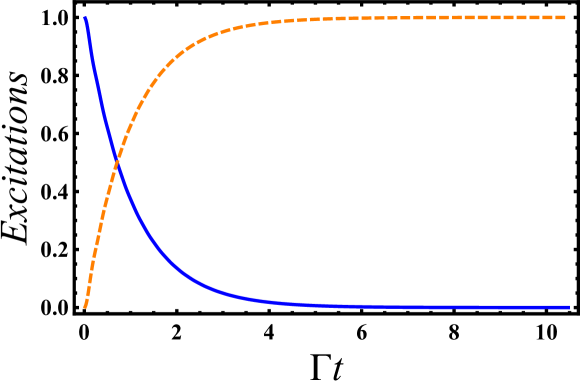
Figure 2: Dynamics of excitations in the main oscillator $(|\alpha(t)/\alpha_{0}|)^{2}$ (blue, solid line) and in the environment $\sum_{k\in E}(|\lambda_{k}(t)/\alpha_{0}|)^{2}$ (orange, dashed line) for the constant coupling case $\gamma=\bar{\gamma}=0.1/30$.

With a non-constant distribution, namely, $\gamma=0.1/30$ and $\bar{\gamma}=50\gamma$, the transfer of excitations oscillates, where the main oscillator is able to take back part of the excitations from the environment (see Fig. 3). After a long enough time, the amplitude of these oscillations decreases until becoming almost null.

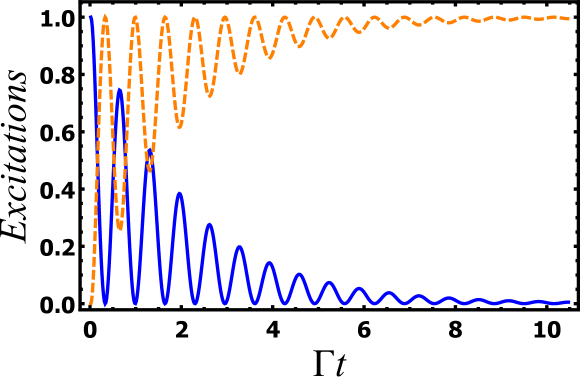
Figure 3: Dynamics of excitations in the main oscillator $(|\alpha(t)/\alpha_{0}|)^{2}$ (blue, solid line) and in the environment $\sum_{k\in E}(|\lambda_{k}(t)/\alpha_{0}|)^{2}$ (orange, dashed line) for non-constant couplings, $\gamma=0.1/30$ and $\bar{\gamma}=50\gamma$.

Observing the excitations behavior, two regimes should be stressed; $\bar{\gamma}=\gamma$ and $\bar{\gamma}>\gamma$. In the first regime, the system excitations are transferred to the environment exponentially. The system is approximately in a Markovian regime (it will only be exactly Markovian in the continuum limit) and almost no “back action” can be observed. In the second regime, the excitations oscillate between the main oscillator and the environment presenting a non-Markovian behavior. This indicates that, in this model, we can go from Markovian to a non-Markovian regime by only changing $\bar{\gamma}$, where the non-Markovian degree can be quantified in terms of this parameter. In the next sections, we will discuss quantum Darwinism in this model and its connection with non-Markovianity.

V The Partial Information Plot approach to the model

For both constant and non-constant coupling cases, we assume in this section the initial state of the main oscillator to be a “cat state,” where we set the parameters $a=1$, $b=1$, $\alpha_{0}=3$, so the global system state is given by

$${|{\Psi(0)}\rangle}=G\left[\left({|{\alpha_{0}}\rangle}+{|{-\alpha_{0}}\rangle}\right)\otimes\prod_{k=1}^{N}{|{0_{k}}\rangle}\right]\noindent,$$ (24)

with

$$G=\frac{1}{\left[2\left(1+e^{-2}\right)\right]^{1/2}}.$$ (25)

It is straightforward to show that

$$|\braket{\alpha(t)}{-\alpha(t)}|^{2} =e^{-2|\alpha(t)|^{2}}$$ (26)

$$\prod_{k\in E}|\braket{\lambda_{k}(t)}{-\lambda_{k}(t)}|^{2} =e^{-2(|\alpha_{0}|^{2}-|\alpha(t)|^{2})},$$ (27)

On the other hand, $\alpha(t)$ is the solution of a linear differential equation with initial condition $\alpha_{0}$, therefore $|\alpha(t)|^{2}$ is proportional to $|\alpha_{0}|^{2}$ for all $t$. Then, from Eqs. (19), (26) and, (27), if $|\alpha_{0}|\gg 1$ and $\Gamma t\sim 1$, we see that states of the system and environment (as a whole) in Eq. (19) are approximately orthogonal, since both $\braket{\alpha(t)}{-\alpha(t)}$ and $\braket{\Lambda(t)}{-\Lambda(t)}$ are $\approx e^{-c|\alpha_{0}|^{2}}$ for some constant $c\sim 1$ independent of $|\alpha_{0}|^{2}$ (for this to be true in the nonconstant coupling case, one must avoid those specific instants of time where all excitations are in the environment). As mentioned in Sec. II, in the quantum Darwinistic regime the environment must monitor a preferential observable of the system. For the quantum Brownian motion studied in Ref. zur2008 , it was essentially the oscillator position. In our model, with the initial state of the system defined in Eq. (24), it is already possible to infer the monitored observable. Indeed, from Eq. (19) and the above discussion, we see that our evolution closely matches that of the von Neumann measurement scheme [see Eq. (1) and subsequent discussion]. Moreover, depending on the (complex) value of $\alpha_{0}$, the system can be monitored in position, momentum, or any quadrature. That is, the environment seems to be performing an approximate homodyne measurement. If $\alpha_{0}$ is a real number, the system will be in a superposition of states with distinct positions, leading the environment to monitor the position. But, if it is a pure imaginary number, the environment will monitor momentum, and so on.

V.1 Constant Coupling

We assume now that $\gamma_{k}=0.1/30$ for all $k$ and the same distribution of frequencies as before. Recall that, as shown in Fig. 2, the excitations of the main oscillator decay exponentially, as expected from the analytical approximation. For large times, therefore, essentially all global system excitations can be found in the environment.

For every fragment $F$, and every instant of time $t$, it is possible to compute the mutual information $I(S:F)$ bet2014 . We then estimate the PIP $\bar{I}(f)$, for each instant of time $t$, by sorting, for each value of $f$, $100$ fragments $F$ with $fN$ subsystems, and averaging the mutual information:

$$\bar{I}(f)\approx\text{avg}_{(\text{random samples of }F)}I(S:F).$$ (28)

Then, we repeated this for fragments composed from $1$ to $900$ ($100\%$) environment oscillators and varied $\Gamma t$ from $0$ to roughly $10$. We note, however, that the mutual information for each $F$ can be computed exactly, exploiting the fact that the reduced density matrix for $S+F$ has rank $2$ for all $F$ (see Ref. bet2014 for details).

The map in Fig. 4 represents the averaged mutual information varying with time and with the environment fraction, $f$. We restrict our analysis in the rest of this section to time windows such that $\Gamma t\sim 6.0$ for all values of $f$. This is reasonable since after this time all system excitations are transferred to the environment and it decouples from the system. After a large enough time, the information about the system will be spread in the bath very redundantly. However the amount of information will be insignificant. Then, more specifically, we will analyze the mutual information, $f_{\delta}$ and $R_{\delta}$ until $\Gamma t=6.0$.

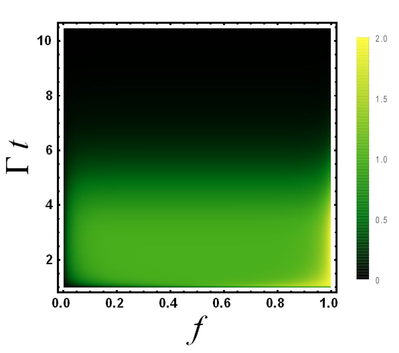
Figure 4: Average mutual information $\bar{I}(f)$ for a constant coupling with $\Gamma t$ going from $0$ to $10$ and the environment fractions $f$ from $1/900$ to $1$.

The signature of quantum Darwinism in the PIP approach is a plateau in the PIP. However, the maximal value of the mutual information can change with time. To compare the shape of each curve we normalize the mutual information for all time values; then, the normalized mutual information $\bar{I}_{N}(f)$ will range from $0$ to $1$. The plot in Fig. 5 shows the PIP for some instants of time, from $\Gamma t=0.03$ to $\Gamma t=6$.

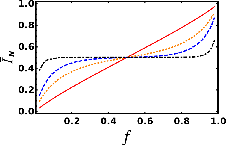
Figure 5: Normalized mutual information $\bar{I}_{N}(f)$ for the constant coupling case. The red (solid), orange (dotted), blue (dashed), and black (dot-dashed) lines represent the PIP for $\Gamma t=0.03$, $\Gamma t=0.17$, $\Gamma t=0.35$, and $\Gamma t=6$, respectively.

For a plateau, the mutual information reaches a relevant value quickly and stabilizes until almost all the environment is taken. In Fig. 5, for a small time ($\Gamma t=0,02$), the mutual information varies almost linearly with the size of the environment fragment (red line). This happens because, in the beginning, just a small amount of correlations were created between the environment and the main oscillator. For larger times, however, not only correlations become more significant, but information about the system is also spread redundantly on the oscillators of the environment. Indeed, in the black dashed dotted line in Fig. 5, the normalized mutual information, as a function of $f$, raises quickly and stabilizes. That is, a small fragment of the environment is enough to obtain almost all information about the preferential observable available in the environment. In this same figure, by the red (solid), orange (dotted), blue (dashed), and black (dot-dashed) lines, it is clear that as $\Gamma t$ grows, the plateau gets more and more pronounced.

As discussed in the Sec. II, a figure of merit of quantum Darwinism is the fraction $f_{\delta}$ and the redundancy, $R_{\delta}$, [see Eq. (3)]. For constant coupling and $\delta=0.05$, we observed that the fraction $f_{\delta}$ decreases rapidly with time, [see inset in the Fig. LABEL:consfrdelta(a)], while, of course, $R_{\delta}$ grows, see Fig. LABEL:consfrdelta(a). However, as time evolves, although the PIP becomes more similar to a plateau, the total information contained in the environment about the system decreases substantially, see Fig. LABEL:consfrdelta(b).

We propose, then, to quantify the redundancy proportionally to the total amount of information about the main oscillator that is available in the environment, namely, $I(S:E)$. We introduce a new quantity, the relative redundancy, $R_{r}$, given by

$$R_{r}(t)=R_{\delta}(t)I(S:E)(t),\noindent$$ (29)

where $I(S:E)(t)$ is the total mutual information between the system and the whole environment at time $t$.

As shown in Fig. LABEL:consfrdelta(c), different from the redundancy, which grows monotonically, the relative redundancy grows with $\Gamma t$ for a maximal value but then decreases to zero.

V.2 Non-Constant Coupling

Starting from the same parameters of Sec. V.1 and the same initial cat state, Eq.(24), we now consider the nonconstant coupling case, varying from a very small to a larger value of $\bar{\gamma}$.

For $\bar{\gamma}>\gamma$, we can see that the excitations oscillates between the main system and the environment. The magnitude of $\bar{\gamma}$ is related to the non-Markovianity of the system and these oscillations represent the backflow of information from the environment to the main system. In Fig. 7(a), PIPs are shown for some instants of time. With $\bar{\gamma}=50\gamma$, at $\Gamma t=0.07$, (red, solid line), the mutual information depends almost linearly on the fragment size $f$. At $\Gamma t=0.52$, (orange, dotted line) and $\Gamma t=1.04$, (blue, dashed line) the plots are closer to a plateau. Lastly, at $\Gamma t=6.0$, (black, dot-dashed line), it is possible to see more clearly a plateau. Observing the strips on the map represented in Fig. 7(b), we can see that this behavior repeats in each cycle.

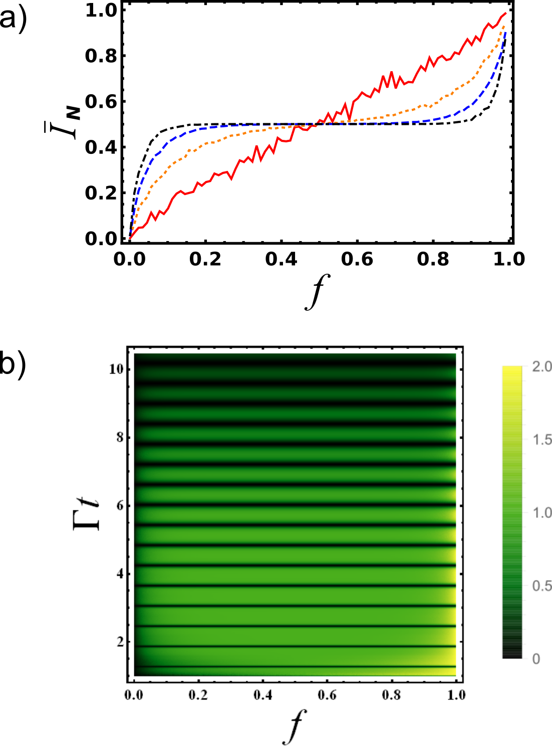
Figure 7: For $\bar{\gamma}=50\gamma$: (a) Mutual Information versus $f$ for $\Gamma t=0.07$ (red, solid line), $\Gamma t=0.52$ (orange, dotted line), $\Gamma t=1.04$ (blue, dashed line) and $\Gamma t=6.0$ (black, dot-dashed line). (b) Map of the mutual information varying with $\Gamma t$ and with $f$.

We have also computed the relative redundancy, $R_{r}$, as a function of time, in the same time window. In Figs. 8 =(a) and (b), it is possible to observe $R_{r}$ as a function of time for two values of $\bar{\gamma}$, with $\delta=0.05$. As the excitations exchange between the main system and environment oscillates in time (the orange dashed line), the redundancy and, consequently, the relative redundancy (the blue solid line) also oscillates with the same frequency. Consequently, the larger $\bar{\gamma}$ is, the larger is the oscillation frequency of $R_{r}$. In each cycle, as the excitations are transferred from the system to the environment, $R_{r}$ increases to a maximal value, and as the excitations flow back to the system, it decreases to a minimal value.

To sum up, in general there is significant redundant information in the environment, except in the vicinity of those instants of time where the oscillator loses all its excitations to the environment, since they also lose all correlations at those instants.

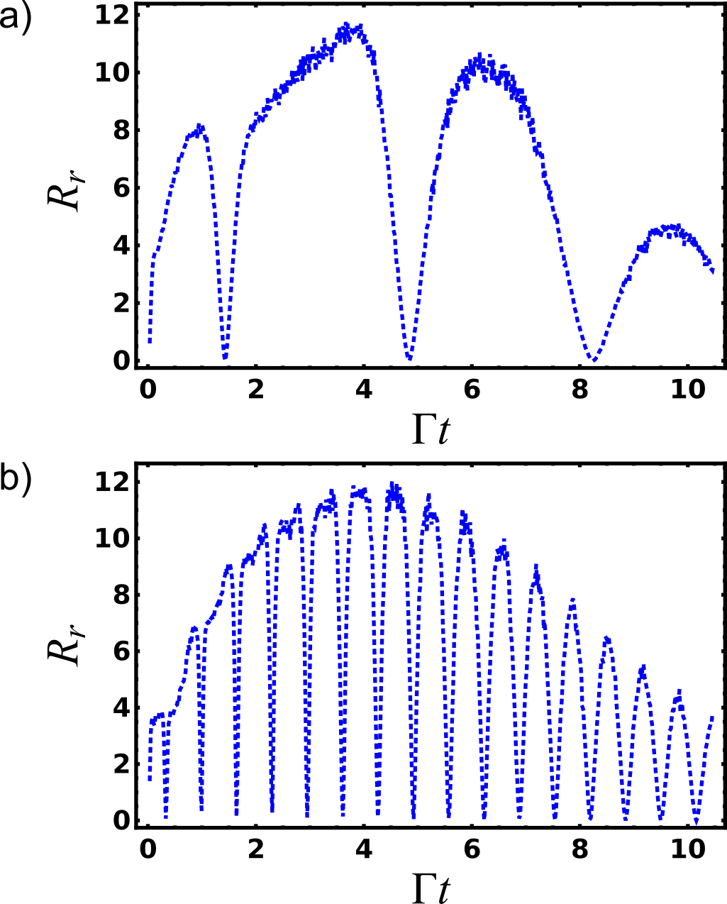
Figure 8: Relative redundancy for $\delta=0.05$ varying with $\Gamma t$ for (a) $\bar{\gamma}=10\gamma$ and (b) $\bar{\gamma}=50\gamma$.

VI The BPH approach to the model

Let us consider again the initial state Eq. (18) with $a$ and $b$ arbitrary. From Eq. (19), we can compute, for every $t$, the mapping from the initial main oscillator states $\rho=G^{2}(a{|{\alpha_{0}}\rangle}+b{|{-\alpha_{0}}\rangle})(a^{*}{\langle{\alpha_{0}}|}+b^{*}{\langle{-\alpha_{0}}|})$ to environment oscillator states:

$$\Lambda_{F}^{t}(\rho) =\text{Tr}_{S,E-F}({|{\Psi(t)}\rangle}\!{\langle{\Psi(t)}|})$$ (30)

$$=G^{2}|a|^{2}\prod_{j\in F}{|{\lambda_{j}(t)}\rangle}\!{\langle{\lambda_{j}(t)}|}$$ (31)

$$+G^{2}|b|^{2}\prod_{j\in F}{|{-\lambda_{j}(t)}\rangle}\!{\langle{-\lambda_{j}(t)}|}$$ (32)

$$+D(t)\prod_{j\in F}{|{\lambda_{j}(t)}\rangle}\!{\langle{-\lambda_{j}(t)}|}+\text{H.c.},$$ (33)

where

$$D(t)=G^{2}ab^{*}\braket{\alpha(t)}{-\alpha(t)}\prod_{j\in E-F}\braket{\lambda_{j}(t)}{-\lambda_{j}(t)}.$$

Now, assuming, as in the previous section, that $|\alpha_{0}|\gg 1$ we see that $\braket{\alpha_{0}}{-\alpha_{0}}=e^{-2|\alpha_{0}|^{2}}\approx 0$ and, therefore, $G\approx 1$. Moreover, we have $|a|^{2}\approx\text{Tr}({|{\alpha_{0}}\rangle}\!{\langle{\alpha_{0}}|}\rho)$ and $|b|^{2}\approx\text{Tr}({|{-\alpha_{0}}\rangle}\!{\langle{-\alpha_{0}}|}\rho)$. Assuming further that $D(t)\approx 0$, we have:

$$\Lambda_{F}^{t}(\rho) \approx\text{Tr}({|{\alpha_{0}}\rangle}\!{\langle{\alpha_{0}}|}\rho)\prod_{j\in F}{|{\lambda_{j}(t)}\rangle}\!{\langle{\lambda_{j}(t)}|}$$ (34)

$$+\text{Tr}({|{-\alpha_{0}}\rangle}\!{\langle{-\alpha_{0}}|}\rho)\prod_{j\in F}{|{-\lambda_{j}(t)}\rangle}\!{\langle{-\lambda_{j}(t)}|}.$$ (35)

Therefore, at least in the subspace generated by ${|{\pm\alpha_{0}}\rangle}$, the maps are approximately a measure and prepare map with the (approximate) POVM $\{{|{\pm\alpha_{0}}\rangle}\!{\langle{\pm\alpha_{0}}|}\}$ and environment states $\sigma_{F,\pm}^{t}=\prod_{j\in F}{|{\pm\lambda_{j}(t)}\rangle}\!{\langle{\pm\lambda_{j}(t)}|}$.

Now, let us check that indeed $D(t)\approx 0$ distinguishes two regimes: $\Gamma t\sim 1$ and $\Gamma t\gg 1$. For the first case, $D(t)$ is indeed small since we have $\braket{\alpha(t)}{-\alpha(t)}=e^{-c|\alpha_{0}|^{2}}\approx 0$ for some $c\sim 1$. Note that for the nonconstant coupling case, not only must we have $\Gamma t\sim 1$ but also consider specific instants of time where the excitations go back to the main oscillator (see Fig. 3).

For $\Gamma t\gg 1$ (but not so large that recurrences can take place due to the finite number of oscillators in the environment), we can assume that all excitations are essentially in the environment. A typical environment fragment $F$ will have then $|\alpha_{0}|^{2}f$ excitations, where $f=|F|/N$ is the fraction of environment systems that this fragment has (see Appendix B). Therefore, the complementary region $E-F$ will have $|\alpha_{0}|^{2}(1-f)$ excitations and we have $\prod_{j\in E-F}\braket{\lambda_{j}(t)}{-\lambda_{j}(t)}\approx e^{-2|\alpha_{0}|^{2}(1-f)}\approx 0$ as long as $f$ is not too close to $1$. Indeed, it holds $D(t)\approx 0$.

Still, in the regime $\Gamma t\gg 1$, the distinguishability between the pure states $\sigma_{F,\pm}^{t}$, which is given by $1-\prod_{j\in F}|\braket{\lambda_{j}(t)}{-\lambda_{j}(t)}|$ can then be approximated by $1-e^{-2|\alpha_{0}|^{2}f}$, and quickly approaches to $1$ with the environment fraction $f$ that is taken. Note that this argument applies for both the constant and non-constant coupling cases. In Appendix B we argue in more detail that this distinguishability will depend essentially on $f$ and $|\alpha_{0}|^{2}$, but not on $\bar{\gamma}$.

To sum up, we see that the first regime, $\Gamma t\sim 1$, resembles the first example given in Sec. II.3, while the asymptotic regime $\Gamma t\gg 1$ resembles the second one, since the global states have a similar structure in each instance, with the correspondences ${|{0(1)}\rangle}\leftrightarrow{|{(-)\alpha(t)}\rangle}$ and ${|{0(1)}\rangle}_{k}\leftrightarrow{|{(-)\lambda_{k}(t)}\rangle}$. For $\Gamma t\sim 1$ there are strong correlations between small environment fractions and the main oscillator which are sufficient to obtain significant information about the preferred observable at instant of time $t$ or its statistics in the initial state, so Darwinism is meaningful here from both the PIP and BPH perspectives. For $\Gamma t\gg 1$, on the other hand, there are essentially no correlations between the environment and the main oscillator, so it is meaningless to address Darwinism from the PIP perspective. However, small environment fragments still keep a record of the statistics of the preferred observable in the main oscillator initial state. So it is still meaningful to address Darwinism from the BPH perspective.

VII Quantum Darwinism and non-Markovianity

In the constant coupling case, there are no excitations returning to the system, and, consequently, no backflow of information, signalizing that the system is Markovian. In the non-constant coupling case, the oscillations of the excitations of the system and the environment show us that these systems are non-Markovian. In particular, it seems that the non-Markovianity of the system raises with the frequency of these oscillations.

We recall the non-Markovianity quantifier in Eq. (12). We estimated this quantity by sorting pairs of initial coherent states for the main oscillator. We chose $1000$ initial complex values of $\alpha_{0}$, according to a normal distribution, and calculated the fidelity of all possible combinations of these states, for different values of $\bar{\gamma}$. As expected, the larger $\bar{\gamma}$ is the larger the non-Markovianity degree will be, see Fig. 9(a).

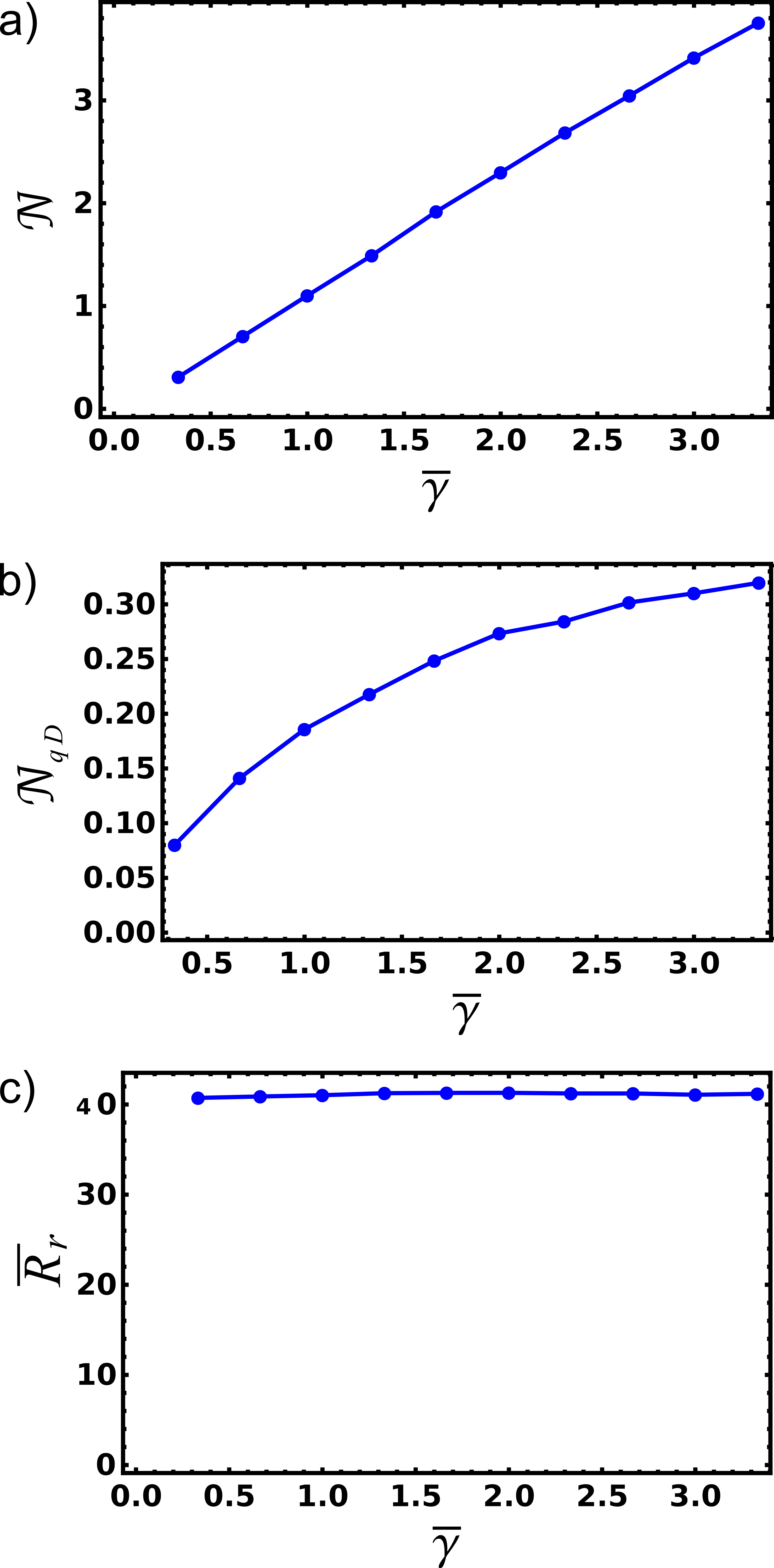
Figure 9: (a) non-Markovianity degree $\mathcal{N}$, (b) Non-monotonicity $\mathcal{N}_{qD}$, and (c) averaged relative redundancy $R_{r}$ versus $\bar{\gamma}$, with $\bar{\gamma}$ going from $10\gamma$ to $100\gamma$. In (a), we sort 1000 initial states coherent states and $\mathcal{N}$ was calculated for all combinations of pairs and in (c) the time interval of the integration is $\Gamma\Delta t=10$.

To understand the connection between quantum Darwinism and non-Markovianity, in Ref. sab2016 the authors quantified the non-monotonic behavior of $f_{\delta}$ that was defined similarly to the non-Markovianity degree:

$$\mathcal{N}_{qD}=\int_{df_{\delta}/dt>0}\frac{df_{\delta}}{dt}dt.\noindent$$ (36)

Note that the integral is calculated just when $df_{\delta}/dt$ is positive. They show that the behavior of $\mathcal{N}_{qD}$ is very similar to the behavior of $\mathcal{N}$, having a good qualitative agreement. So, they concluded that quantum Darwinism is being hindered by non-Markovianity.

We also calculated this quantity in our model and we could observe that $\mathcal{N}_{dD}$ as a function of $\bar{\gamma}$ grows monotonically as $\mathcal{N}$, see Fig. 9(b). This is expected since as non-Markovianity grows, more oscillations in the redundancy and $f_{\delta}$ will be present. Then, if we integrate the values of $f_{\delta}$ just when it is growing, the non-monotonicity will increase with the oscillation frequency and therefore, with $\bar{\gamma}$.

Although this analogy is consistent, we present here a different point of view. We could observe in non-Markovian systems that the oscillations of the excitations lead to oscillations in the redundancy. When the excitations are being transferred to the environment, the redundancy grows. When the excitations are flowing back to the system the redundancy decreases. Nevertheless, even in the moments of backflow of excitations, we can say that there exists some redundancy in the system and, therefore, some degree of quantum Darwinism. We believe then that a more sensitive figure of merit would be the averaged relative redundancy $R_{r}(\bar{\gamma})$ for a certain period of time $\Delta t=t\text{max}-t\text{min}$, that is,

$$\bar{R}_{r}(\bar{\gamma})=\frac{1}{\Delta t}\int_{t\text{min}}^{t\text{max}}R_{r}(t,\bar{\gamma})dt.\noindent$$ (37)

We calculated this quantity for different values of $\bar{\gamma}$ in a time window $\Gamma\Delta t=10$ . The result is presented in Fig. 9(c) and it show us that the values of $\bar{R}_{r}(\bar{\gamma})$ are practically constant. This implies that, for any random instant of time, the probability to find quantum Darwinism in the Markovian case is nearly the same of the case of high non-Markovianity. Putting in another way, even if the amount of quantum Darwinism is non-monotonic in time in a non-Markovian dynamics, on average, it is the same as in the Markovian case.

We can also relate the two concepts from the BHP perspective. As discussed in Sec. IV, in the asymptotic regime $\Gamma t\gg 1$, all excitations initially in the main oscillator go to the environment. Their distribution in the environment, however, depends strongly on $\bar{\gamma}$. Since the non-Markovianity of the main oscillator dynamics depends only on $\bar{\gamma}$, the asymptotic state of the environment actually keeps a record of the non-Markovianity. On the other hand, as pointed out in Sec. VI, and detailed in Appendix B, the asymptotic environment state redundant recording of the main oscillator preferred observable (the quantum Darwinism from the BHP perspective) is essentially independent of $\bar{\gamma}$.

VIII Conclusions

We studied quantum Darwinism from two distinct perspectives and its connection with non-Markovianity in a system made of a single quantum harmonic oscillator coupled to an environment of a large set of quantum harmonic oscillators. Through the calculations of mutual information between the system and fragments of the environment with different sizes, we could see that the environment monitors the system constantly and we could check the existence or not of quantum Darwinism at each instant of time. We analyzed the mutual information varying with the environment fragment size and the relative redundancy. This was done also varying a parameter of the model that controls the degree of non-Markovianity of the main oscillator dynamics.

In the Markovian case, we verified that, after correlations are established between the system and the environment, indeed the information about the preferred observable is distributed redundantly through the environment. However, in the non-Markovian case, the excitations and the relative redundancy oscillates. As the non-Markovianity increases, more oscillations takes place. In both cases, however, it is noticeable that the environment monitors the system instantly.

In Ref. sab2016 , the authors study the consequences of non-Markovianity on quantum Darwinism through the non-monotonicity of $f_{\delta}$, quantified by $\mathcal{N}_{f}$. There, the value of $f_{\delta}$ is integrated just when $\dot{f}_{\delta}$ is growing. It was shown that this quantity increases with the non-Markovianity degree, suggesting that quantum Darwinism is being hindered by it. We could observe a similar result in our model.

We offer in this paper a different point of view to relate non-Markovianity and quantum Darwinism. In the time instants where the excitations are being transferred from the system to the environment, correlations between them are created, spreading redundant information about the system in the environment. This also causes a rise in the redundancy. As expected in a non-Markovian system, the oscillations will cause a backflow of information from the environment to the system. When the environment “gives back” part of the information for the system, a part of the correlation early created is also destroyed, leading to a decrease of the redundancy. In these moments, it is also possible to see the relative redundancy decreasing. However, as the transfer of excitations oscillates, the correlations turn to grow up and this cycle repeats. Then, since quantum Darwinism can be observed in cycles, even when it is decreasing, it makes sense to consider it in all instants of time. Then, to quantify the effect of non-Markovianity on quantum Darwinism, we computed the averaged relative redundancy $R_{r}$, that consists of the relative redundancy averaged on a period of time, for different values of $\bar{\gamma}$. We observed that there is no clear correlation between $R_{r}$ and $\bar{\gamma}$, leading us to conclude that as long the system and environment are exchanging excitations, the observation of the quantum Darwinism depends just on the particular instant of time of the analysis.

Finally, even in the asymptotic limit, it is possible to address quantum Darwinism from the BPH perspective, even though there is no correlations between the main oscillator and its environment. It is also possible to address non-Markovianity in this limit, since the distribution of excitations in the environment is sensitive to the non-Markovianity of the main oscillator dynamics. Then, we have seen that, also from this perspective, that quantum Darwinism in this regime is essentially independent from the non-Markovianity degree.

Appendix A Exact solution through a continuum limit approximation

As mentioned in section IV, the model admits an analytical for the continuum limit Eq. (22). Then, one is able to solve Eqs. (16) and Eq.(17) by formally integrating (17), substituting in Eq. (16), leading to an integro-differential equation that is easy to solve in the continuum limit. The result is then:

$$\alpha(t) = \alpha_{0}e^{-\Gamma t/2},$$ (38)

$$\lambda(\omega,t) = i\alpha_{0}\gamma\frac{e^{\left(-\Gamma/2+i\Delta\omega\right)t}}{\Gamma/2+i\Delta\omega},\noindent$$ (39)

where $\Delta\omega=\omega_{0}-\omega$ and $\Gamma=4\pi\gamma^{2}\rho$ [recall Eq. (23)].

In the asymptotic limit, the environment excitations distribute like a Lorenztian centered at $\omega_{0}$:

$$|\lambda(\omega,t\rightarrow\infty)|^{2}\rho=|\alpha_{0}|^{2}\frac{1}{\pi}\frac{\Gamma}{(\Gamma/2)^{2}+(\omega-\omega_{0})^{2}}.$$ (40)

For the nonconstant coupling case, by a similar procedure, one arrives at:

$$\alpha(t)=\frac{\alpha_{0}}{2\Omega}e^{-\Gamma t/4}\left[\Gamma/4\left(e^{-\Omega t}-e^{\Omega t}\right)\right.$$

$$+\left.\Omega\left(e^{-\Omega t}+e^{\Omega t}\right)\right],$$ (41)

$$\lambda(\omega_{0},t)=\frac{i\alpha_{0}\bar{\gamma}}{2\Omega}e^{-\Gamma t/4}\left(e^{-\Omega t}-e^{\Omega t}\right),$$ (42)

$$\lambda(\omega,t)=\frac{-i\alpha_{0}\gamma}{2\Omega}\left[\frac{\left(\Gamma/4+\Omega\right)\left(1-e^{-\left(\Gamma/4+i\Delta\omega+\Omega\right)t}\right)}{\Gamma/4+i\Delta\omega+\Omega}\right.$$

$$+\left.\frac{\left(\Gamma/4-\Omega\right)\left(1-e^{-\left(\Gamma/4+i\Delta\omega-\Omega\right)t}\right)}{-\Gamma/4-i\Delta\omega+\Omega}\right],\noindent$$ (43)

with $\Omega=\sqrt{(\Gamma/4)^{2}-\bar{\gamma}^{2}}$. From these expressions we get that, in the asymptotic limit and for $\bar{\gamma}\gg\Gamma$, the environment excitations distribute approximately as a sum of two Lorentzians centered at $\omega_{0}+\bar{\gamma}$ and $\omega_{0}-\bar{\gamma}$:

$$|\lambda(\omega,t\rightarrow\infty)|^{2}\rho \approx\frac{|\alpha_{0}|^{2}}{4\pi}[\frac{\Gamma}{(\Gamma/4)^{2}+(\omega-(\omega_{0}+\bar{\gamma}))^{2}}$$

$$+\frac{\Gamma}{(\Gamma/4)^{2}+(\omega-(\omega_{0}-\bar{\gamma}))^{2}}].$$ (44)

Appendix B Distinguishability of states of sampled environment subsystems

We have discussed the analytical solution to the model in the continuum limit in Sec. IV and Appendix A. We recall that there is a well-defined asymptotic distribution of excitations in the reservoir, that is $\lim_{t\rightarrow\infty}|\lambda(\omega,t)|^{2}\rho$ exists for all $\omega$. For $\bar{\gamma}=\gamma$, the Markovian regime, we have a Lorentzian distribution of width $\Gamma$ [see Eq. (40)], while for $\bar{\gamma}\gg\Gamma$, deep in the non-Markovian regime, we have essentially a sum of two Lorentzians of width $\Gamma/2$ [see eq. (44)]. Even though we consider a model with a finite number of oscillators in the environment, this analytical solution serves as guide and a good approximation to understand the finite case.

We have seen in Sec. VI that, for an initial global state $G(a{|{\alpha_{0}}\rangle}+b{|{-\alpha_{0}}\rangle})\otimes\prod_{k}{|{0}\rangle}_{k}$, the mapping between the initial system state and the state of environment fragment $F$ at instant $t$ satisfies Eq. (35), which we reproduce here for convenience:

$$\Lambda_{F}^{t}(\rho)\approx\text{Tr}({|{\alpha_{0}}\rangle}\!{\langle{\alpha_{0}}|}\rho)\prod_{k\in F}{|{\lambda_{k}(t)}\rangle}\!{\langle{\lambda_{k}(t)}|}$$ (45)

$$+\text{Tr}({|{-\alpha_{0}}\rangle}\!{\langle{-\alpha_{0}}|}\rho)\prod_{k\in F}{|{-\lambda_{k}(t)}\rangle}\!{\langle{-\lambda_{k}(t)}|}.$$ (46)

The distinguishability between the environment states appearing in these expressions depends essentially on the number of excitations in the environment fraction $F$, that is, $\sum_{k\in F}|\lambda_{k}(t)|^{2}$. We shall consider $F\subset E$, with $|F|=f/N$ for fixed $f>0$, as elements of a sample space with uniform probability distribution, with each $F$ having probability $1/\binom{N}{fN}$, where $\binom{N}{fN}$ is the binomial coefficient. We would like to understand a random variable of the form

$$X(F)=\sum_{k\in F}p_{k},$$ (47)

where $p_{k}=|\lambda_{k}(T)|^{2}$ for some fixed (independent of $N$) $T\gg 0$. It holds that $\sum_{i=1}^{N}p_{k}=|\alpha_{0}|^{2}:=p$ holds exactly for all $T$ and the constant $p$ is independent of $N$.

Basically, we want to show the distribution of $X$ to be highly concentrated around its average value, if $N$ is large enough.

It is easy to check that the expectation value of $X$ satisfies

$$\mathbb{E}(X)=\frac{1}{\binom{N}{fN}}\sum_{F\subset E}\sum_{k\in F}p_{k}=pf,$$ (48)

regardless of the functional dependence of $p_{k}$ on $k$.

We shall consider first a a prototype distribution for the distribution we have in the Markovian case [which is the Lorentzian Eq. (40) in the continuum limit]. Namely, for some fixed $0<a<1$, $p_{k}=p/Na$ for $|k/N-1/2|<a/2$ and $p_{k}=0$ otherwise. That is, the graph of $p_{k}$ has a rectangular shape of width $a$, height $p/Na$, centered at $N/2$. Let $[N]=\{1,...,N\}$ and let $J=\{k\in[N]||k/N-1/2|<a/2\}$, that is, $J$ is the set of indexes where $p_{k}\neq 0$. The value of $X(F)$ will then be defined by $|F\cap J|$, that is, the number of indexes of $F$ that are in $J$. Now, if we think the points of $F$ as “particles” that we can uniformly distribute in a large “box” $[N]$, that was divided in two parts, a smaller box $J$ versus the rest $[N]-J$, we have a standard problem in statistical mechanics. It is well known that the density of particles in $J$, $|F\cap J|/aN$ will be highly concentrated, in probability, around its average value $f$. Namely, for any $\epsilon>0$, it holds that, for sufficiently large $N$,

$$\mathbb{P}(|\frac{|F\cap J|}{aN}-f|)>\epsilon\leq be^{-cN}$$ (49)

for some positive constants $b$ and $c$ that depends on $f$ and $a$. Since $X(F)=\frac{p}{aN}|F\cap J|$, we then get:

$$\mathbb{P}(|X-pf|)>p\epsilon\leq be^{-cN}.$$ (50)

That is, for the vast majority of environment fractions $F$ with $fN$ subsystems, the total number of excitations in those fractions will be very close to $f|\alpha_{0}|^{2}$.

We can also consider a prototype distribution in the same spirit, but for the non-Markovian case [a sum of two Lorentzians, in the continuum limit and for $\bar{\gamma}\gg\Gamma$, see Eq. (44)]. Namely, for some fixed $0<a<1$, $p_{k}=p/Na$ for $|k/N-1/4|<a/4$ or $|k/N-3/4|<a/4$, and $p_{k}=0$ otherwise. In this case, the graph of $p_{k}$ has the shape of two rectangles of width $a/2$, height $p/Na$, one centered at $N/4$, the other at $3N/4$. Nevertheless, the exact same reasoning as before applies and we get exactly the same bound Eq. (50).