Scalar induced resonant sterile neutrino production in the early Universe

Abstract

It has been recently suggested [1, 2] that a cosmic scalar field can completely change the keV-scale sterile neutrino production in the early Universe. Its effect may, for various parameter choices, either suppress sterile neutrino production and make moderate active-sterile mixing cosmologically acceptable, or increase the production and generate considerable dark matter component out of sterile neutrino with otherwise negligible mixing with SM. In this paper we provide analytic estimates complementing and providing details of the numerical calculations performed in [2] in the case of resonant amplification of the sterile neutrino production. We also discuss phenomenological and theoretical issues related to the successful implementation of this idea in fully realistic extensions of the Standard Model of particle physics.

INR-TH-2019-021

1 Introduction

The numerous dark matter phenomena getting gradually accepted [3] ask for either modification of General Relativity or extension of the Standard Model of particle physics (SM). In the latter case of a special interest are those extensions which are motivated by particle physics itself, independently from cosmology. These extensions must contain a new electrically neutral, stable at cosmological time-scales particles and provide a mechanism operating in the early Universe to produce them in a sufficient amount. That is to yield a relative contribution of the new species (several in case of multicomponent dark matter) $\Omega_{M}\simeq 0.27$ to the present energy density of the Universe.

One of the well-motivated candidates to form one of the dark matter components is sterile neutrinos — singlet with respect to SM gauge group fermions, inducing neutrino masses via mixing with the SM (or active) neutrinos. In this way neutrino oscillations get explained, see e.g. [4, 5]. The sterile-active mixing makes sterile neutrino unstable. Consequently, the sterile neutrinos decay via weak interactions into light SM particles, with the decay into three active neutrinos being always open. However, since the weak decay rate goes with the decaying particle mass $M_{X}$ as $\Gamma_{W}\propto M_{X}^{5}$, sufficiently light sterile neutrinos may be long-lived enough to survive till the present, with the lifetime exceeding the Universe age $\tau_{U}\simeq 1.4\times 10^{10}$ y. This is one of the necessary conditions of a dark matter component. It selects keV-mass scale as cosmologically viable, provided the sterile-active mixing is enough for the sterile neutrino contributing to active neutrino mass, for details see e.g. [6, 7]. However, at present, this chain of arguments is misleading actually, as we explain below.

Remarkably, the instability suggests a specific signature of the sterile neutrino dark matter: it radiatively decays into active neutrino and photon. This two body decay implies a peak feature in the Galactic photon spectrum at the energy of half of the sterile neutrino mass ($X$-rays for the keV mass-scale). Extensive searches for this peak (which relative width is of order $10^{-3}$ due to the Doppler shift of an object bound by the Galaxy gravity force) revealed no signal so far, and severely constrained the sterile neutrino model parameter space. These searches place upper limits on the active-sterile mixing at a given sterile neutrino mass, under the assumption of all the dark matter being formed by the sterile neutrino only. These bounds do not depend on a mechanism of the sterile neutrino production operating in the early Universe, but if sterile neutrino is only a subdominant dark matter component, the limits are correspondingly weaker.

The relic sterile neutrinos must be produced in the early Universe at some stage of its expansion in the amount right enough to form the entire dark matter component, or at least its fraction. The production mechanisms, based on active-sterile neutrino oscillations in the primordial plasma provide with sterile neutrino of momenta proportional to the plasma temperature. Hence, the keV-scale neutrinos form so-called warm dark matter [6], a dark matter variant subjecting to specific constraints from the cosmic structure formation [8] and from phase space density [9, 10]. Together with X-ray searches, the most recent one is [11], these constraints exclude the simplest mechanism of sterile neutrino production via the oscillations in the primordial plasma [12] and leave only small regions in the model parameter space cosmologically viable in the situation when the primordial plasma is asymmetric with respect to the lepton charge [13]. While the latter case is still allowed (e.g. within the $\nu$MSM setup), the sterile neutrino there does not contribute enough to active neutrino masses, and one may ask for other mechanisms, either extensions or alternatives to those mentioned above. To our knowledge none of the suggested in literature mechanisms simultaneously explains the active neutrino masses via mixing and produces the full dark matter component consistent with cosmological and astrophysical bounds discussed above.

The sterile neutrinos of keV-mass range are most efficiently produced in the oscillations at temperature of about 100 MeV [12]. Therefore, to amplify or suppress the production via oscillations one can respectively increase or decrease the effective sterile-active mixing in the primordial plasma at this epoch. As we pointed out in Refs. [1, 2], the latter effect can be achieved by coupling the sterile neutrino to a scalar field with specific homogeneous evolution in the expanding Universe . With a constant scalar field this coupling can make the sterile neutrino either massless or superheavy in the interesting epoch, thus naturally preventing the sterile neutrino production [1]. Alternatively, rapidly oscillating scalar can resonantly amplify the neutrino oscillations [2] and enhance the sterile neutrino production in comparison with the standard case [12]. The periodically varying scalar field can induce a parametric resonance phenomenon which dramatically increases the amplitude of neutrino oscillations regardless of active-sterile mixing. This mechanism has been studied numerically in Ref. [2], which showed that the small (as compared to the standard case) sterile-active mixing may be sufficient to produce enough dark matter. This observation justifies a further search for the peak-like signature in the $X$-rays with the next-generation telescopes such as eRosita and ART-XC on the base of Spektr-RG platform [16, 17].

Parametric resonance phenomenon in systems coupled to the oscillating background is not a novel in particle physics. In one of the pioneering studies [18] devoted to neutron–antineutron oscillations in a periodically varying magnetic field a strong enhancement of the probability amplitude was explored. Later, amplification of spin-flavor neutrino oscillations in electromagnetic fields of various configurations was found in Ref. [19]. In Ref. [20] the method for the investigation of the neutrino evolution equation solution near the resonance point was suggested. A novel approach to study neutrino oscillations in the presence of general rapidly varying fields without assumptions about the strength of the time-varying external field was developed in Ref. [21]. Instead of solving the evolution equation directly the author has derived the new effective Hamiltonian which described the evolution of the averaged neutrino wave function. In contrast to Ref. [20], the elaborated method was beyond the perturbation treatment and applicable for arbitrary strength of the external field. However, a new approach requires a large frequency of the time-varying background compared to that of the system at the absence of any external force. For this reason, it is instructive to explore the resonance dynamics of neutrino oscillations in the presence of oscillating background in different assumption about external conditions. In this sense, our analysis is complementary to one in Ref. [21] and can be used to examine the parametric resonance phenomenon at a different choice of model parameters.

In this paper we develop the analytic approach to describe the resonant dynamics, estimate the amount of and calculate the spectrum of the produced dark matter sterile neutrinos. This study represents a logical extension of the previous analysis [2]. We corroborate the numerical treatment of Ref. [2] with rigorous analytical approach which allows to extend the scope of our mechanism and provides proper analytic understanding of the dependence of cosmological predictions on the model parameters. In particular, we generalise the framework of Ref. [2] in the presence of thermal environment which allows to examine resonance dynamics in the high temperature regime.

The paper is organized as follows. In Section 2 we describe the oscillating sterile-active neutrino system in the expanding Universe as the Schroedinger equation with external field and find the resonance solution. In Section 3 we suggest an analytic approximation to the spectrum of resonantly produced sterile neutrinos. Section 4 contains the analytic estimate of the total amount of produced in this way sterile neutrino dark matter. We apply here all the cosmological and astrophysical constraints on the model parameters. Section 5 is devoted to discussion of various issues to be resolved on the way of implementation of the developed mechanism of sterile neutrino production in the realistic extensions of the SM (e.g. seesaw type I with Majorana field or secluded scalar sector). We summarize our results in Conclusion, Section 6. Some lengthy analytic estimates are presented in Appendix A for convenience.

2 Neutrino resonance induced by oscillating background

Our model Lagrangian contains three essential parts:

$$\mathcal{L}=\mathcal{L}_{N}+\mathcal{L}_{\phi N}+\mathcal{L}_{\phi}\,.$$ (2.1)

The first one describes oscillations between active neutrino $\nu$ and its right-handed sterile counterpart $N$ (fermion singlet with respect to the SM gauge group) in vacuum. It reads

$$\mathcal{L}_{N}=i\bar{\nu}\hat{\partial}\nu+i\bar{N}\hat{\partial}N+\frac{M}{2}\bar{N^{c}}N+m_{D}\bar{\nu}_{a}N+\text{h.c.}.$$ (2.2)

where $m_{D}$ is the Dirac mass appeared after the electroweak transition and equals

$$m_{D}=\theta M$$ (2.3)

where $\theta$ is the mixing angle in vacuum (i.e. at present, in the cosmological context) and $M$ is the bare mass of sterile neutrino. The Dirac term implies the second non-zero mass eigenvalue of the $\nu$-$N$ system, the active neutrino mass of order $m_{a}\sim m_{D}^{2}/M\sim\theta^{2}M$. The second ingredient of our model (2.1) is the real scalar field $\phi$ (the SM singlet as well) which feebly couples to sterile neutrino via Yukawa like interaction

$$\mathcal{L}_{\phi N}=\frac{f}{2}\,\phi\bar{N^{c}}N+\text{h.c.}$$ (2.4)

The Yukawa term (2.4) gives rise to the time-dependent contribution

$$M_{N}=f\phi(t)$$ (2.5)

to the effective sterile neutrino mass

$$M_{\rm eff}\equiv M+M_{N}.$$ (2.6)

It implies that the scalar field treated as an external force here may control the neutrino oscillations in the early Universe. The corresponding impact is determined by dynamic of the scalar sector. To simplify the analysis we will use the theory of free massive scalar field

$$\mathcal{L}_{\phi}=\frac{1}{2}(\partial_{\mu}\phi)^{2}+\frac{1}{2}m_{\phi}^{2}\phi^{2}$$ (2.7)

In this framework, at early times the scalar field is frozen and the sterile neutrinos can be very heavy (2.5)

$$M_{N,i}=f\phi_{i}.$$ (2.8)

When the Universe expansion rate (i.e. the Hubble parameter) drops below $H_{{\rm osc}}\simeq m_{\phi}$ the scalar field begins to oscillate that results in the variable sterile neutrino mass contribution (2.5) oscillating with frequency $m_{\phi}$ (2.5)

$$M_{N}=M_{A}\sin m_{\phi}t.$$ (2.9)

and decreasing amplitude

$$M_{A}\equiv M\left(\frac{hT^{3}}{h_{e}^{\vphantom{3}}T_{e}^{3}}\right)^{\!1/2}\,.$$ (2.10)

Hereafter we assume the Universe at radiation domination and parameterize the amplitude (2.10) so, that at the temperature $T=T_{e}$ it coincides in value with the bare mass $M_{N}$.

In what follows we study the dynamics of active-to-sterile neutrino transitions in the presence of oscillating scalar field coupled to the sterile massive state. Sum of (2.2) and (2.4) can be rewritten in a more contracted form (2.5), (2.6)

$$\begin{split}\mathcal{L}_{N}+\mathcal{L}_{\phi N}=i\bar{\mathcal{N}}_{L}\hat{\partial}\mathcal{N}_{L}&+\frac{1}{2}\bar{\mathcal{N}}_{L}^{c}\begin{pmatrix}0&m_{D}\\ m_{D}&M_{\rm eff}\end{pmatrix}\mathcal{N}_{L}+\text{h.c.},\\ \mathcal{N}_{L}&\equiv\begin{pmatrix}\nu\\ N^{c}\end{pmatrix}\end{split}$$ (2.11)

or in terms of Majorana fields $\mathcal{N}\equiv\left(\mathcal{N}_{L}+\mathcal{N}_{L}^{c}\right)/\sqrt{2}$ it reduces to

$$\begin{split}\mathcal{L}_{N}+\mathcal{L}_{\phi N}=i\bar{\mathcal{N}}\hat{\partial}\mathcal{N}&+\bar{\mathcal{N}}\begin{pmatrix}0&m_{D}\\ m_{D}&M_{\rm eff}\end{pmatrix}\mathcal{N}.\end{split}$$ (2.12)

Massive part of (2.12) can be diagonalized by the following orthogonal transformation

$$\begin{split}\mathcal{O}=&\begin{pmatrix}\cos\theta_{\rm eff}&\sin\theta_{\rm eff}\\ -\sin\theta_{\rm eff}&\cos\theta_{\rm eff}\end{pmatrix}\end{split}$$ (2.13)

where effective time-dependent mixing $\theta_{\rm eff}$ is defined through

$$\tan\theta_{\rm eff}=\frac{2m_{D}}{M_{\rm eff}+\sqrt{M_{\rm eff}^{2}+4m^{2}_{D}}}.$$ (2.14)

Upon transformation $\mathcal{N}=\mathcal{O}\mathcal{V}$ (2.13) Lagrangian (2.12) arrives at

$$\begin{split}\mathcal{L}_{N}+\mathcal{L}_{\phi N}=i\bar{\mathcal{V}}\hat{\partial}\mathcal{V}+&i\mathcal{V}^{\dagger}\begin{pmatrix}0&\dot{\theta}_{\rm eff}\\ -\dot{\theta}_{\rm eff}&0\end{pmatrix}\mathcal{V}+\bar{\mathcal{V}}\begin{pmatrix}m_{1}&0\\ 0&m_{2}\end{pmatrix}\mathcal{V},\\ m_{1,2}&=\frac{M_{\rm eff}}{2}\left(1\mp\sqrt{1+4\frac{m_{D}^{2}}{M_{\rm eff}^{2}}}\right),\end{split}$$ (2.15)

and squared mass difference of (2.15) reads

$$\Delta m^{2}=M_{\rm eff}^{2}\sqrt{1+\frac{4m_{D}^{2}}{M_{\rm eff}^{2}}}$$ (2.16)

To describe evolution of the two-level system (2.15) in the presence of oscillating background (2.6), (2.9) we employ matrix form of the Schrödinger equation. Evolution of massive neutrino states in vacuum under the most general assumptions is governed by (2.15)

$$i\frac{\partial}{\partial t}\begin{pmatrix}\nu_{1}\\ \nu_{2}\end{pmatrix}=\begin{pmatrix}-\Delta_{0,{\rm eff}}/2&-i\dot{\theta}_{\rm eff}\\ i\dot{\theta}_{\rm eff}&\Delta_{0,{\rm eff}}/2\end{pmatrix}\begin{pmatrix}\nu_{1}\\ \nu_{2}\end{pmatrix}$$ (2.17)

where $\nu_{1}$, $\nu_{2}$ denote wave functions of massive states and we also defined the effective rate of neutrino oscillations in vacuum (2.16)

$$\Delta_{0,{\rm eff}}\equiv\frac{\Delta m^{2}}{2p}$$ (2.18)

Analysis of neutrino oscillations via (2.17) is rather involved. Framework (2.17) can be simplified significantly under several assumptions. First, if effective angle (2.14) changes slowly enough, the massive states $\nu$ can be treated as stationary and possible convertions $\nu_{1}\leftrightarrow\nu_{2}$ can be neglected. The corresponding adiabacity condition reads

$$\frac{|\dot{\theta}_{\rm eff}|}{\Delta_{0,{\rm eff}}}\ll 1\,.$$ (2.19)

Assuming (2.19) the original framework (2.17) for massive states can be rewritten in the flavour basis using transformation $(\nu_{1},\nu_{2})^{\rm T}=\mathcal{O}^{-1}(\psi_{1},\psi_{2})^{\rm T}$ (2.13) as follows

$$i\frac{\partial}{\partial t}\begin{pmatrix}\psi_{1}\\ \psi_{2}\end{pmatrix}=\mathcal{H}\begin{pmatrix}\psi_{1}\\ \psi_{2}\end{pmatrix}$$ (2.20)

where $\psi_{1}$, $\psi_{2}$ refer to the flavour basis and the effective Hamiltonian reads

$$\mathcal{H}=\frac{\Delta_{0,{\rm eff}}}{2}\left(\begin{array}[]{cc}-\cos 2\theta_{\rm eff}&\sin 2\theta_{\rm eff}\\ \sin 2\theta_{\rm eff}&\cos 2\theta_{\rm eff}\end{array}\right).$$ (2.21)

Second, in addition to (2.19) one can require smallness of effective mixing (2.14). Assuming

$$\frac{2m_{D}}{M_{\rm eff}}\ll 1\,,$$ (2.22)

we found simplified forms of oscillating parameters (2.16), (2.14), (2.3)

$$\begin{split}\Delta m^{2}&\approx M_{\rm eff}^{2}\,,\\ \sin^{2}\theta_{\rm eff}&\approx\frac{m_{D}}{M_{\rm eff}}\,.\end{split}$$ (2.23)

Assuming (2.23) and exploiting the following notations

$$\Delta_{0,{\rm eff}}\equiv 2\beta(z+\sin m_{\phi}t)^{2},\qquad\beta\equiv\frac{M_{A}^{2}}{4p}\,,\qquad z\equiv\frac{M}{M_{A}}\,,$$ (2.24)

eq. (2.20) reduces to

$$i\frac{\partial}{\partial t}\begin{pmatrix}\psi_{1}\\ \psi_{2}\end{pmatrix}=\beta(z+\sin m_{\phi}t)^{2}\begin{pmatrix}-1&\frac{\displaystyle 2\theta z}{\displaystyle z+\sin m_{\phi}t}\\ \frac{\displaystyle 2\theta z}{\displaystyle z+\sin m_{\phi}t}&1\end{pmatrix}\begin{pmatrix}\psi_{1}\\ \psi_{2}\end{pmatrix}.$$ (2.25)

Additional assumptions (2.19), (2.22), whose validity is exhaustively discussed in Appendix A, allow one to reduce the rather complicated framework (2.17) to a more straightforward dynamics governed by (2.25). To solve the latter we introduce the basis flavour states in the absence of mixing: $|\psi_{a}\rangle=\begin{pmatrix}\psi_{1}^{(0)}\\ 0\end{pmatrix}$ and $|\psi_{s}\rangle=\begin{pmatrix}0\\ \psi_{2}^{(0)}\end{pmatrix}$. These states can be easily founded as solutions of the diagonal part of the Schrodinger equation (2.25), namely $\psi_{1,2}^{(0)}=e^{\pm i\beta\int_{0}^{t}(z+\sin m_{\phi}\zeta)^{2}d\zeta}$.

So, the state vector $|\psi(t)\rangle\equiv\begin{pmatrix}\psi_{1}\\ \psi_{2}\end{pmatrix}$ at any moment can be presented in the following form

$$|\psi(t)\rangle=y_{1}(t)|\psi_{a}\rangle+y_{2}(t)|\psi_{s}\rangle,$$ (2.26)

where $y_{1}(t)$ and $y_{2}(t)$ are corresponding flavour amplitudes

$$\begin{split}y_{1}(t)=\langle\psi_{a}|\psi(t)\rangle,\\ y_{2}(t)=\langle\psi_{s}|\psi(t)\rangle.\end{split}$$ (2.27)

We are interested in the so-called appearance probability of the sterile state, so we put $|\psi(0)\rangle=|\psi_{a}\rangle$. In this case $y_{1}(t)$ and $y_{2}(t)$ describe survival and transition amplitudes, respectively.

Substituting (2.26) into (2.25) gives rise to the following system of equations on flavour amplitudes (2.27)

$$\begin{cases}\frac{\displaystyle\partial y_{1}(t)}{\displaystyle\partial t}=-2i\beta z\theta(z+\sin m_{\phi}t)e^{-2i\beta\int_{0}^{t}(z+\sin m_{\phi}\zeta)^{2}d\zeta}y_{2}(t)\\ \frac{\displaystyle\partial y_{2}(t)}{\displaystyle\partial t}=-2i\beta z\theta(z+\sin m_{\phi}t)e^{2i\beta\int_{0}^{t}(z+\sin m_{\phi}\zeta)^{2}d\zeta}y_{1}(t)\end{cases}$$ (2.28)

with initial conditions $y_{1}(0)=1$, $y_{2}(0)=0$.

In what follows we work in the limit of small energy transfer between the active and sterile states, that means

$$|y_{2}(t)|\ll 1\,.$$ (2.29)

In this approximation the number density of active neutrinos reduces insignificantly during all oscillation period $y_{1}(t)\simeq 1$. This assumption allows one to obtain the solution of (2.28) in the following form

$$y_{2}(t_{1})\simeq-2i\beta z\theta\int_{0}^{t_{1}}(z+\sin m_{\phi}t)e^{2i\beta\int_{0}^{t}(z+\sin m_{\phi}\zeta)^{2}d\zeta}dt\,.$$ (2.30)

The outer integration in (2.30), over $t$, can be carried out with a help of stationary phase method. This method is valid only for significantly large ratios $2\beta/m_{\phi}$. We assume that to apply this strategy one needs at least the equality

$$m_{\phi}\leqslant\beta$$ (2.31)

to be true. Further calculations can be simplified in the regime of large scalar field amplitude, that requires $M\ll M_{A}$ or, given (2.24),

$$z\ll 1\,.$$ (2.32)

2.1 Resonant solution

Denoting

$$\begin{split}h(t)&\equiv 2\int_{0}^{t}(z+\sin m_{\phi}\zeta)^{2}d\zeta,\\ g(t)&\equiv z+\sin m_{\phi}t\,,\end{split}$$ (2.33)

the condition $h^{\prime}(t_{l})=0$ brings the following stationary points $t_{l}$

$$(z+\sin m_{\phi}t_{l})=0$$ (2.34)

or, adopting (2.32),

$$m_{\phi}t_{l}\approx-(-1)^{l}z+\pi l\,.$$ (2.35)

We start with the estimate of the contribution of the second order stationary point $t_{l}\in[0,t_{1}]$ to (2.30). To achieve that one should accomplish the following integration (2.33)

$$\begin{split}\int_{t_{l}-\delta}^{t_{l}+\delta}g(t)e^{i\beta h(t)}dt\approx g^{\prime}(t_{l})e^{i\beta h(t_{l})}\int_{t_{l}-\delta}^{t_{l}+\delta}&(t-t_{l})e^{i\frac{1}{6}\beta(t-t_{l})^{3}h^{\prime\prime\prime}(t_{l})}dt\,.\end{split}$$ (2.36)

For that we make use of the asymptotic methods that yields the following reference integrals [22]

$$\begin{split}\int_{0}^{\delta}t\,e^{ixt^{3}}dt&\sim\frac{1}{3}\,\Gamma\left(\frac{2}{3}\right)x^{-2/3}e^{i\pi/3},\qquad\,\,x\rightarrow+\infty\\ \int_{-\delta}^{0}t\,e^{ixt^{3}}dt&\sim-\frac{1}{3}\,\Gamma\left(\frac{2}{3}\right)x^{-2/3}e^{-i\pi/3},\quad x\rightarrow+\infty\end{split}$$ (2.37)

Using (2.37), the asymptotic expansion of (2.36) in the limit $2\beta/m_{\phi}\rightarrow+\infty$ reduces to

$$\int_{t_{l}-\delta}^{t_{l}+\delta}g(t)e^{i\beta h(t)}dt\sim ig^{\prime}(t_{l})\,\frac{\sqrt{3}}{3}\,\Gamma\left(\frac{2}{3}\right)\left(\frac{6}{\beta|h^{\prime\prime\prime}(t_{l})|}\right)^{2/3}e^{i\beta h(t_{l})}.$$ (2.38)

Assuming the amplitude (2.38) and approximations

$$\begin{split}h^{\prime\prime\prime}(t_{l})&=4m_{\phi}^{2}\left(\cos 2m_{\phi}t_{l}-z\sin m_{\phi}t_{l}\right)\approx 4m_{\phi}^{2}\\ g^{\prime}(t_{l})&=m_{\phi}\cos m_{\phi}t_{l}\approx(-1)^{l}\,m_{\phi}\end{split}$$ (2.39)

we write down the contribution of $l$-th stationary point to the integral (2.30)

$$\left.y_{2}\right|_{l}\!=\!2z\theta(-1)^{l}\sqrt{3}\,\Gamma\!\left(\frac{2}{3}\right)\!\left(\!\frac{\beta}{12m_{\phi}}\!\right)^{1/3}\!\!\exp\left\{i\frac{2\beta}{m_{\phi}}\left(\frac{\displaystyle\pi l(1\!+\!2z^{2})}{\displaystyle 2}\!+\!2z(1\!-\!(-1)^{l})\right)\!\right\}.$$ (2.40)

To estimate the intagral (2.30) over large periods of time one needs to sum up contributions (2.40) over the all stationary points (2.35) encountered in the time interval $[0,t_{1}]$, namely $\sum\left.y_{2}\right|_{l}$. To attain this goal, we split $\sum\left.y_{2}\right|_{l}$ into odd and even parts as follows,

$$\sum \left.y_{2}\right|_{l}=\sum_{l=2k}\left.y_{2}\right|_{l}+\sum_{l=2k+1}\left.y_{2}\right|_{l},$$

$$\sum_{l=2k}\left.y_{2}\right|_{l}=2z\theta\sqrt{3}\,\Gamma\!\left(\frac{2}{3}\right) \left(\!\frac{\beta}{12m_{\phi}}\!\right)^{1/3}\sum_{k=0}^{l_{\rm max}/2}\!\exp\left\{\displaystyle i\frac{2\beta}{m_{\phi}}\cdot\pi k(1\!+\!2z^{2})\right\},$$ (2.41)

$$\sum_{l=2k+1}\!\!\left.y_{2}\right|_{l}=-2z\theta\sqrt{3}\,\Gamma\!\left(\frac{2}{3}\right) \left(\!\frac{\beta}{12m_{\phi}}\!\right)^{1/3}\sum_{k=0}^{l_{\rm max}/2}\!\exp\left\{i\frac{2\beta}{m_{\phi}}\left(\frac{\pi(2k\!+\!1)}{2}(1\!+\!2z^{2})\!+\!4z\right)\!\right\},$$

where $l_{\rm max}$ refers to the final time $t_{1}$, see (2.35), as

$$l_{\rm max}\approx\frac{m_{\phi}t_{1}}{\pi}\,.$$ (2.42)

The sums in (2.41) are geometric progressions with the common ratio $\exp\{i\frac{2\beta}{m_{\phi}}\pi(1+2z^{2})\}$. The growing mode in the solution $\left|\sum\left.y_{2}\right|_{l}\right|$ refers to the following condition: $\\ \beta(1+2z^{2})/m_{\phi}\in\mathbb{N}$ or (2.24), that is

$$\frac{M_{A}^{2}+2M^{2}}{4p_{n}}=nm_{\phi},\quad n\in\mathbb{N}\,.$$ (2.43)

The condition (2.43) guarantees a parametric resonance in the two-level system when the mass of one state is modulated by oscillating background. The integer $n$ parameterizes diversity of the parametric resonances in such a system. This situation refers to the most prominent conversions $\nu_{a}\rightarrow\nu_{s}$.

Eventually, assuming (2.42), (2.43), (2.24) we simply reduce (2.41) to the leading order in $z$ (2.32) as

$$|y_{\rm 2,lin}(t)|\approx\left|\sum\left.y_{2}\right|_{l}\right|\approx 0.65\,\theta\,m_{\phi}t\frac{M}{M_{A}}n^{1/3}\begin{cases}|\sin 4\frac{M}{M_{A}}n|,\quad\text{for even}\,\,n\\ |\cos 4\frac{M}{M_{A}}n|,\quad\text{for odd}\,\,n\end{cases}$$ (2.44)

In order to demonstrate the applicability of our theoretical approach, we confront the analytical approximation (2.44) with numerical solution of equations (2.28) for resonances with various values of $n$, see (2.43). Fig. 1 shows that our estimate (red line) in the regime (2.29) reproduces the numerical solution (blue line) very precisely for $n=10$ and more modestly in case $n=1$. However, this nice accordance is broken if one examines the resonant behaviour at $y_{2}(t)\lesssim 1$. Given this reason, one needs to find a proper solution of (2.28) which does not rely on (2.29). To achieve this goal we examine, for particular sets of variables, one phenomenological dependency $|\sin y_{\rm 2,lin}(t)|$ (green dashed line) against numerical solution (blue line) in Fig. 1. The performed analysis reveals that the first oscillation peak of the numerical solution is approximated by this phenomenological model reasonably well. Thus, a proper solution in the case of resonance (2.43) which does not rely on (2.29) is given by (2.44)

$$y_{\rm 2,res}(t)\approx\left|\sin\left(\frac{\omega_{\rm res}\cdot t}{2}\right)\right|,$$ (2.45)

where

$$\omega_{\rm res}\approx 1.3\,\theta\,m_{\phi}\frac{M}{M_{A}}n^{1/3}\begin{cases}|\sin 4\frac{M}{M_{A}}n|,\quad\text{for even}\,\,n\\ |\cos 4\frac{M}{M_{A}}n|,\quad\text{for odd}\,\,n\end{cases}$$ (2.46)

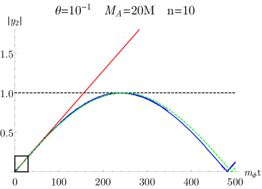
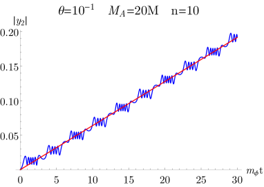
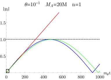
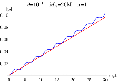
Figure 1: The blue line represents the numerical solution of equations (2.28). The red line depicts our analytical approximation (2.44) in the regime (2.29). The green dashed line refers to our phenomenological result (2.45).

Our phenomenological result (2.45) manifests a good resemblance with that of the numerical approach for any integer $n$, see (2.43). It justifies the application of stationary phase method and reveals its efficiency to describe the parametric resonance in the two-level system (2.28).

2.2 Width of resonance

The other important characteristics of a parametric resonance is its width. To obtain a range of momenta for which the flavour amplitudes deviate from their resonant values moderately, we calculate (2.30) in some vicinity of $n$-resonance (2.43) provided by

$$\frac{M_{A}^{2}+2M^{2}}{4p_{n}}=(n+\alpha)m_{\phi}\,,$$ (2.47)

where $\alpha\ll 1$. Using the stationary phase method elaborated in Sec. 2.1 we reduce (2.41) to the following amplitude (2.42), (2.47)

$$|y_{2,\alpha}(t)|\approx 0.65\,\theta\,m_{\phi}\frac{M}{M_{A}}n^{1/3}\frac{2\pi\left|\sin\left(\frac{m_{\phi}\alpha}{2}t+\pi\alpha\right)\right|}{|\sin\pi\alpha|}\begin{cases}|\sin(4\frac{M}{M_{A}}n+\frac{\pi\alpha}{2})|,\quad\text{for even}\,\,n\\ |\cos(4\frac{M}{M_{A}}n+\frac{\pi\alpha}{2})|,\quad\text{for odd}\,\,n\end{cases}$$ (2.48)

As expected, in the extremely small vicinity of resonance, i.e. at $\alpha\rightarrow 0$, our result (2.48) reproduces the linear resonant solution (2.44) under assumption of (2.29).

To find the relevant value of parameter $\alpha$ which governs (2.47), we introduce the absolute value of amplitude $y_{2}(t)$

$${\rm max}\,|y_{2}|\approx\left|y_{2,\alpha}\left(\frac{\pi}{m_{\phi}\alpha}\right)\right|.$$ (2.49)

Assuming $\alpha\ll 1$ and $2\theta\frac{M}{M_{A}}n^{1/3}\ll{\rm max}\,|y_{2}|$ we can express $\alpha$ through ${\rm max}\,|y_{2}|$ in the following form (2.48)

$$\alpha\approx\frac{1}{{\rm max}\,|y_{2}|}\,\frac{\omega_{\rm res}}{m_{\phi}}\,.$$ (2.50)

Then, adopting (2.49), (2.50) in the vicinity of resonance (2.47), the solution (2.48) can be presented as

$$|y_{2,\alpha}(t)|\approx{\rm max}\,|y_{2}|\times\left|\sin\left(\frac{\omega\cdot t}{2}\right)\right|,$$ (2.51)

where

$$\omega\approx\frac{\omega_{\rm res}}{{\rm max}\,|y_{2}|}\,.$$ (2.52)

We recall that our results obtained above rely on the small energy transfer condition (2.29). However, the final outcome (2.51) in the limit ${\rm max}\,|y_{2}|\rightarrow 1$ matches the evolution at the resonance (2.45). It suggests that our result (2.51) can be applied for arbitrary value of $y_{2}(t)$ if only its amplitude ${\rm max}\,|y_{2}|$ is treated as a free parameter and its relation with (2.50) is not exploited. To verify this statement, we confront our estimate (2.51) with the numerical solution (2.28) of the same amplitude for various values of ${\rm max}\,|y_{2}|$ and $n$. Fig. 2 reveals that our approach (dashed green line), indeed, can be applied even for a big enough ${\rm max}\,|y_{2}|$.

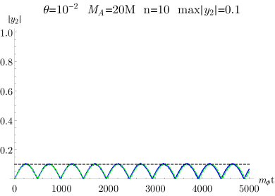
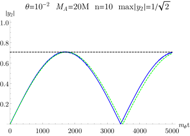
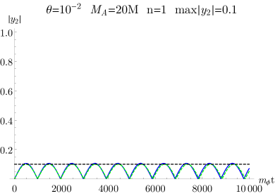
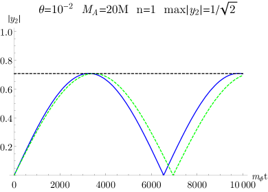
Figure 2: The blue line represents the numerical solution of equations (2.28) on the amplitude ${\rm max}\,|y_{2}|$. The green dashed line depicts our estimate (2.51) of the same amplitude ${\rm max}\,|y_{2}|$. The black dashed line shows the chosen value ${\rm max}\,|y_{2}|$ in each case.

Eventually, we define a range of momenta, $\Delta p_{n}\equiv|p-p_{n}|$, for which ${\rm max}\,|y_{2}|>1/\sqrt{2}$ holds via (2.47):

$$\Delta p_{n}=\frac{\alpha|_{1/\sqrt{2}}}{n}p_{n}\,,$$ (2.53)

where $\alpha|_{1/\sqrt{2}}$ relates to (2.50) at ${\rm max}\,|y_{2}|=1/\sqrt{2}$ . Thus, the width of resonance reads (2.53)

$$\frac{\Delta p_{n}}{p_{n}}\simeq\frac{\sqrt{2}}{n}\frac{\omega_{\rm res}}{m_{\phi}}\,.$$ (2.54)

For our choice of parameters (2.32) the resonance (2.43) is narrow, $\Delta p_{n}/p_{n}<1$. It implies that the neutrino conversion in the resonance might be inefficient once one considers expansion of the Universe. The latter effect gives rise to a particular feature in the spectrum of sterile neutrinos produced in resonance that is the subject of Sec. 3. But before moving forward we study the resonance behaviour in the presence of a dense environment composed of the thermally-populated SM particles.

2.3 Plasma effect

The results obtained above are based on the vacuum oscillation framework. However, at high temperatures the active neutrino propagates through dense cosmological plasma that affects oscillations. This effect may be crucial for the resonant behaviour at high temperatures. Given this reason, we generalise our results obtained in Sec. 2.1 and 2.2 in the presence of matter.

The forward scattering of active neutrino in the thermal bath induces the following effective Hamiltonian (2.21)

$$\mathcal{H}_{\rm eff}=\mathcal{H}-\left(\begin{array}[]{cc}V&0\\ 0&0\end{array}\right),$$ (2.55)

where $V$ denots effective potential for active neutrinos in the plasma. We consider the mixing of sterile state only with electron neutrino and vanishing initial primordial lepton number, so [23]

$$V\approx 63\times\Gamma\,,\qquad\Gamma\approx 1.27\times G_{F}^{2}T^{4}p\,.$$ (2.56)

In what follows we consider significantly high scalar field values and examine matter effects in the following reasonable assumption,

$$V\ll\frac{M_{A}^{2}}{4p}\,.$$ (2.57)

Then one can apply the stationary phase method elaborated in Sec. 2.1 directly to effective Hamiltonian (2.55) and obtain the following resonant condition in the plasma,

$$\frac{M_{A}^{2}+2M^{2}}{4p_{n}}+V=nm_{\phi}\,,\quad n\in\mathbb{N}\,.$$ (2.58)

This relation generalizes the resonance condition in vacuum (2.43) and provides a bit different neutrino momentum at the resonance $p_{n}$ assuming (2.57). In turn, the resonance solution in the presence of matter matches that in the vacuum (2.45) and exhibits the same frequency (2.46). This means that in assumption of (2.57) the plasma effects do not affect the resonant behavior and introduce only a slight offset in the resonance condition (2.58). The contribution of this displacement is not significant either, if one enquires about the average resonant momentum $p_{n}$ provided by (2.58) in the assumption of (2.57).

Finally, using the numerical analysis based on (2.20), (2.55), (2.21) with precise oscillation parameters (2.14), (2.16) we verified that our analytical approach elaborated in Sec. 2.1 and 2.2 works reasonably well until

$$5M\lesssim M_{A}\,,$$ (2.59)

$$5V\lesssim\frac{M_{A}^{2}}{4p}$$ (2.60)

become valid, see (2.10), (2.56).

3 Spectrum with narrow resonance

Expansion of the Universe eventually moves the system through the region , where the resonance condition for a particular mode (2.43) is fulfilled, that can thereby provide with meaningful sterile neutrino abundance. In particular, redshift effect gives rise to time-dependency of resonant conformal momentum $y_{n}$ passing through $n$-resonance at temperature $T$ (2.43)

$$y_{n}\equiv\frac{p_{n}}{T}\approx\frac{M_{A}^{2}}{4Tm_{\phi}}\frac{1}{n}\,.$$ (3.1)

The whole band of the width $\Delta y_{n}=\Delta p_{n}/T$ (2.54) moves through a given resonant momentum $y_{n}$ (3.1) over time

$$\delta t_{n}=\frac{\Delta y_{n}}{\dot{y}_{n}}=\frac{1}{n}\frac{\omega_{\rm res}}{\sqrt{2}m_{\phi}H}\,.$$ (3.2)

If this period is shorter than typical time of resonant oscillations $\omega_{\rm res}^{-1}$, the resonance becomes ineffective ("narrow"). This happens at high temperature when

$$\frac{\sqrt{2}m_{\phi}H}{\omega_{\rm res}^{2}}n>1\,.$$ (3.3)

The l.h.s. of (3.3) describes the efficiency of $n$-resonance at temperature $T$ in the expanding Universe. Hence, this quantity can be used to parametrize the spectrum of sterile neutrinos produced in the case of "narrow" resonance. First, we recover the asymptotic behaviour of sterile neutrino distribution function in several limits of (3.3) on theoretical grounds. Second, we resort to numerical analysis and build the interpolating solution for sterile neutrino spectrum valid for any reasonable value of parameter (3.3).

In the static limit, $n\sqrt{2}m_{\phi}H/\omega_{\rm res}^{2}\ll 1$, the amount of sterile neutrino reaches the Fermi–Dirac distribution after typic time $\omega_{\rm res}^{-1}$ (2.45), so

$$\frac{f_{N}}{f_{FD}}\simeq 1\,.$$ (3.4)

In the opposite limit, $n\sqrt{2}m_{\phi}H/\omega_{\rm res}^{2}\gg 1$, the generation of sterile neutrinos is strongly suppressed. The production rate in the resonance is given by the frequency of corresponding solution $\omega_{\rm res}$, see (2.45). However, the "narrow" resonance terminates earlier due to the strong expansion effect over $\delta t_{n}\ll\omega_{\rm res}^{-1}$ (3.2). Thereby, the distribution function of the generated during one "narrow" resonance sterile neutrinos is given by $f_{N}/f_{FD}\simeq\omega_{\rm res}\delta t_{n}$ or (3.2)

$$\frac{f_{N}}{f_{FD}}\simeq\left(\frac{\sqrt{2}m_{\phi}H}{\omega_{\rm res}^{2}}n\right)^{-1}$$ (3.5)

To find solution interpolating between these two limits (3.4) and (3.5) we solve matrix-valued generalizations of the Boltzmann equations called density matrix equations [24]

$$i\frac{\partial}{\partial t}\rho=[\mathcal{H},\rho]-\frac{i}{2}\{\Gamma_{A},\rho-\rho_{\mathrm{eq}}\}$$ (3.6)

where $\rho$ is the 2x2 density matrix corresponding to active and sterile neutrinos, with $\rho_{11}$ ($\rho_{22}$) being the probability density of the active (sterile) neutrino. Here $\rho_{\mathrm{eq}}=\mathrm{diag}(f_{\mathrm{FD}}(y),f_{\mathrm{FD}}(y))$ is the equilibrium Fermi-Dirac distribution and $\Gamma_{A}=\left(\begin{array}[]{cc}\Gamma&0\\ 0&0\end{array}\right)$ is the damping term due to active neutrino interactions in the thermal bath. The evolution starts at early times with $\rho=\mathrm{diag}(f_{\mathrm{FD}}(y),0)$ and the interesting distribution of the produced sterile neutrinos is obtained as $f_{N}(y)=\rho_{22}(y)$ at late times, $t\to\infty$. We exploit the Hamiltonian in vacuum (2.21) since its thermal modification brings only sub-dominant contribution in accordance with Sec. 2.3. We also employ precise oscillation parameters (2.14), (2.18), (2.16).

We work in the limit $\omega_{\rm res}\gg H$, so the redshift effect in (3.6) can be addressed by the following linear expansion

$$\begin{split}p&=\tilde{p}(1-Ht)\\ M_{A}&=\tilde{M}_{A}(1-\frac{3}{2}Ht)\end{split}$$ (3.7)

where $\tilde{p}$ and $\tilde{M}_{A}$ refer to the moment of resonance (2.43).

Solving (3.6), (2.21), (3.7) for various values of l.h.s. of (3.3) yields the sterile neutrino distribution function. Results of this numerical analysis for various model parameters are shown in Fig. 3.

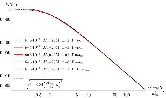
Figure 3: $f_{\mathrm{FD}}/f_{N}$ as a function of l.h.s. of (3.3). Dashed black line refers to our fitting result (3.8).

Matching of $f_{N}/f_{FD}$ for various values $\theta$, $M_{A}/M$, $n$ and $\Gamma$ demonstrates stability and universal dependency of the solution on l.h.s. of (3.3) which parametrizes the "narrow" resonance in the expanding Universe. We also verified that $f_{N}/f_{FD}$ is insensitive to $m_{\phi}$ and to absolute value of $M$.

For a proper usage we fit our numerical result with the following analytical function

$$f_{N}=\frac{f_{\mathrm{FD}}}{\sqrt{1+0.84\left(\frac{\displaystyle\sqrt{2}m_{\phi}H}{\displaystyle\omega_{\rm res}^{2}}n\right)^{2}}}.$$ (3.8)

where $\sqrt{2}m_{\phi}H/\omega_{\rm res}^{2}$ refers to the moment of resonance (2.43). Since the temperature unambiguously corresponds to a particular resonant conformal momentum via (3.1), our result (3.8) can be presented in a more conventional form (2.46) [2]

$$f_{N}(y)=\frac{f_{\mathrm{FD}}(y)}{\sqrt{1+0.84\left(\frac{\displaystyle y}{\displaystyle y_{s}}\right)^{5}}}\,.$$ (3.9)

where cut-off scale $y_{s}$ is defined by

$$y_{s}=\frac{0.24}{n^{17/15}}\left(\frac{\theta}{4.2\cdot 10^{-6}}\right)^{4/5}\!\!\left(\frac{\!M}{\!\,\text{keV}}\right)^{2}\!\!\left(\frac{9.3\,\text{MeV}}{T_{e}}\right)^{9/5}\!\!\left(\frac{\,\text{eV}}{m_{\phi}}\right)^{3/5}\!\!\left(\frac{50}{g_{*,s}}\right)^{1/5}\!\!\left(\frac{h_{s}}{h_{e}}\right)^{3/5}.$$ (3.10)

The mode, corresponding to $y_{s}$ passes through the resonance (2.43) at temperature (3.1), (3.10)

$$T_{s}=\frac{28\,\text{MeV}}{n^{1/15}}\left(\frac{\theta}{4.2\cdot 10^{-6}}\right)^{2/5}\!\!\left(\frac{T_{e}}{9.3\,\text{MeV}}\right)^{3/5}\!\!\left(\frac{m_{\phi}}{\,\text{eV}}\right)^{1/5}\!\!\left(\frac{50}{g_{*,s}}\right)^{1/10}\!\!\left(\frac{h_{e}}{h_{s}}\right)^{1/5}$$ (3.11)

The net results is given approximately by the sum of (3.9) over resonances $n=1,2,\dots$. However, one observes from (3.10) that the higher resonances are relevant at lower neutrino momentum. The most prominent contribution both to neutrino abundance and to the average neutrino velocity comes from the lowest resonance $n=1$. This case is studied in the next Section.

4 Sterile neutrino dark matter

In this section we consider sterile neutrino DM that is produced in resonance and has spectrum (3.9). The correct DM neutrino abundance, in this case, can be achieved only if the resonant conformal momentum (3.10) is small enough. Since higher resonances are relevant at lower neutrino momentum (3.10), resonance with the highest momentum ($n=1$) gives the most important contribution both to the neutrino abundance and to the average neutrino velocity. Given this reason, we neglect any contribution of higher resonances ($n>1$) and examine sterile neutrino production in resonance with $n=1$ only.

The proper abundance of DM composed of sterile neutrinos of spectrum (3.9) is achieved for [2]

$$y_{s}\simeq 0.24\times\left(\frac{1\,\text{keV}}{M}\right)^{2/5}.$$ (4.1)

The sterile neutrino distribution function (3.9) for this cutoff is shown in Fig. 4.

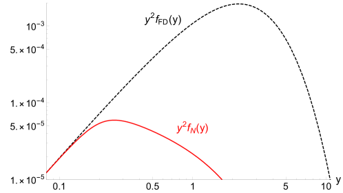
Figure 4: The Fermi–Dirac $f_{\mathrm{FD}}$ and sterile neutrino $f_{N}$ spectra in logarithmic scale.

The characteristic feature in the sterile neutrino distribution function at $y\gtrsim y_{s}$ provides a cool spectrum with average

$$\langle\!\langle y\rangle\!\rangle=0.6\left(\frac{50}{g_{*,s}}\right)^{1/3}$$ (4.2)

where $g_{*,s}$ refers to the plasma effective degrees of freedom at the reference temperature of sterile neutrino production $T\simeq T_{s}$. Such a feature allows to alleviate structure formation constraints on the mass of DM particle. Ly-$\alpha$ constraint $m_{\rm NRP}>8\,\text{keV}$ [6] is translated in our case to

$$M>1.5\,\text{keV}\left(\frac{50}{g_{*,s}}\right)^{1/3}.$$ (4.3)

4.1 Parameter constraints

Here we examine the available parameter region $(\theta^{2},M)$ where the sterile neutrinos with spectrum (3.9), (4.2) is capable of composing all the present dark matter. For that, we should address all relevant constraints.

For the purpose of this Section one can equate (4.1) and (3.10) that leads to

$$\theta\sim 4.2\times 10^{-6}\left(\frac{1\,\text{keV}}{M}\right)^{3}\left(\frac{g_{*,s}}{50}\right)^{1/4}\left(\frac{T_{e}}{9.3\,\text{MeV}}\right)^{9/4}\left(\frac{m_{\phi}}{1\,\text{eV}}\right)^{3/4}\left(\frac{h_{e}}{h_{s}}\right)^{3/4}$$ (4.4)

Further, we assume that sterile neutrino DM is effectively produced at temperature $T\simeq T_{s}$ (3.1), (4.1)

$$T_{s}=3T_{e}\left(\frac{T_{e}}{9.3\,\text{MeV}}\right)^{1/2}\left(\frac{m_{\phi}}{1\,\text{eV}}\right)^{1/2}\left(\frac{1\,\text{keV}}{M}\right)^{6/5}\left(\frac{h_{e}}{h_{s}}\right)^{1/2}.$$ (4.5)

Since we explore here parameter space $(\theta^{2},M)$, it is convenient to rewrite (4.5) in the following form (4.4)

$$T_{s}=28\,\text{MeV}\left(\frac{\theta}{4.2\cdot 10^{-6}}\right)^{2/3}\left(\frac{M}{\,\text{keV}}\right)^{4/5}\left(\frac{50}{g_{*,s}}\right)^{1/6}.$$ (4.6)

One of the most rigorous foundations of our theoretical framework refers to the assumption of significantly large scalar field values. To address (2.59) at the moment of sterile neutrino production we require $T_{e}<3T_{s}$, see (2.10). In addition, we always assumed that the active neutrinos equilibrate in the thermal bath, so the parameter space should meet $1\,\text{MeV}<T_{e}$. Finally, $T_{e}$ is confined within

$$1\,\text{MeV}<T_{e}<\frac{T_{s}}{3}\,.$$ (4.7)

To provide small thermal modifications and address (2.60) we impose (2.56), (2.10), (4.1), (4.5)

$$\left.5V\frac{4yT}{M_{A}^{2}}\right|_{\begin{subarray}{c}y=y_{s}\\ T=T_{s}\end{subarray}}<1$$ (4.8)

At $T\simeq T_{e}$ the regime of high scalar field amplitude (2.32) terminates and the common scenario of the non-resonant production via active-sterile oscillations in plasma [12] is resumed. Sterile neutrino amount produced at $T<T_{e}$ should be relativily small,

$$\Omega_{N,T<T_{e}}<\Omega_{\rm DM},$$ (4.9)

where $\Omega_{N,T<T_{e}}$ denotes the corresponding sterile neutrino contribution, generated at $T<T_{e}$ ($M_{\rm eff}\approx M$), for details see [1].

To avoid the effective scalar decay to sterile neutrinos we limit the mass scale as

$$m_{\phi}<M$$ (4.10)

When the mass of scalar field belongs to the interval $0.01\,\text{eV}\approx\sqrt{\Delta m_{\rm sol}^{2}}<m_{\phi}<M$, the scalar field can decay to active neutrinos. This moment relates to $H\sim\Gamma_{\phi\rightarrow\nu\nu}=f^{2}m_{\phi}/16\pi$ and hence happens when the at the temperature $T\simeq T_{\rm dec}$ such that

$$\frac{T_{\rm dec}}{T_{0}}=\frac{\theta^{2}}{4\sqrt{\pi}}\,\frac{f}{\Omega_{\rm rad}^{1/4}}\left(\frac{m_{\phi}}{H_{0}}\right)^{1/2}\left(\frac{g_{*,0}}{g_{*,{\rm dec}}}\right)^{1/4}.$$ (4.11)

This decay channel does not affect sterile neutrino production at $T\simeq T_{s}$ if the corresponding decay is late enough (4.11), (4.5), i.e.

$$T_{\rm dec}<T_{s}$$ (4.12)

We suggest that the perturbative treatment is applied to the scalar field sterile neutrino interaction and hence assume that (4.14)

$$f<1\,.$$ (4.13)

It’s worth noting that the Yukawa coupling (2.4) enters conditions (4.12) and (4.13) only. As we are interested in the most extended attainable region in model parameter space, one can fix $f$ in its lower boundary coming from the dark matter overproduction constraint, $\Omega_{\phi}<\Omega_{\rm DM}$,

$$f_{\rm min}^{2}=\frac{m_{\phi}^{2}M^{2}}{2\Omega_{DM}\rho_{\mathrm{crit}}}\frac{h_{0}T_{0}^{3}}{h_{e}T_{e}^{3}}.$$ (4.14)

Finally, sterile neutrino dark matter should be astrophysically viable. That means, the vacuum mixing must agree with X-ray constraint

$$\theta<\theta_{\rm X-ray}(M).$$ (4.15)

4.2 Results

At each point of parameter space $(\theta^{2},M)$ we look over $\langle T_{e},m_{\phi}\rangle$ and find optimal parameters which address (4.15), (4.7), (4.8), (4.9), (4.10), (4.12) and (4.13) satisfactory. As a result of this procedure we find the most extended available region on the plane ($M,\sin^{2}2\theta$), which is depicted in Fig. 5.

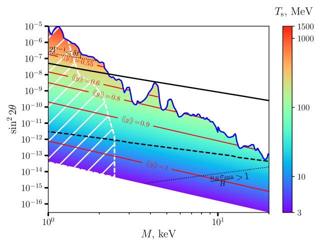
Figure 5: Parameter scan over the sterile neutrino mass and active-sterile mixing angle (the corresponding scalar masses $10^{-2}\,\text{eV}<m_{\phi}<M$ help to avoid additional production of sterile neutrinos from scalar decays at $T\simeq m_{\phi}$ as in Refs.  [25, 26, 27] and $1\,\text{MeV}<T_{e}<150\,\text{MeV}$). The blue line is the upper limit from X-ray observations [11, 28, 29]. The colour region gives the fraction of the sterile neutrino equal to DM, $\Omega_{N}=\Omega_{DM}$. The colour indicates the reference temperature of the sterile neutrino production $T_{s}$ (4.6). The white dashed region is excluded by studying the cosmic structure formation. Red lines refers to sterile neutrino average momenta per temperature calculated just before active neutrino freezeout (4.2). For reference: the black line is for the conventional non-resonant generation mechanism [6], black dashed line corresponds to the maximal lepton asymmetry attainable in the $\nu$MSM [6], upper dotted line relates to equality of (4.16), lower dotted line corresponds to equality of (5.1).

The lower boundary on the mixing angle in the plot of Fig. 5 refers to $T_{s}=3T_{e}=3\,\text{MeV}$, see (4.7). At lower values of $\theta$ the temperature $T_{e}$ drops below $1\,\text{MeV}$ and with the active neutrino out of equilibrium our analysis becomes more involved. The maximum possible mixing angle, in turn, is defined by X-ray constraint (4.15). Condition (4.9) requires $T_{e}\lesssim 150\,\text{MeV}$ above the non-resonant production line [2] which does not affect our region in the model parameter plane ($M,\sin^{2}2\theta$): the corresponding constraint on $\theta$ is always weaker than that from the X-ray in Fig. 5.

One comment is in order here. Numerical analysis carried out in Sec. 3 holds in case of small enough interaction rates, namely $\Gamma<\omega_{\rm res}$. However, the resonances which bring the bulk contribution to the sterile neutrino dark matter are narrow, see (3.9), (4.1). It implies that typical time of neutrino conversions in resonance is small compared to $\omega_{\rm res}^{-1}$ and the corresponding constraint on $\Gamma$ is weaker. All in all, the interaction rate does not affect the oscillations in resonance if the interaction length in plasma surpasses the typic time of resonant oscillations (3.2), i.e.

$$2\Gamma^{-1}>\delta t_{1}$$ (4.16)

We outline the region where condition (4.16) is broken by dotted line in the top part of Fig. 5. The parameter space above this line cannot be reliably described by outcomes of Sec. 3 and needs a more sophisticated approach which accounts for interplay between flavor oscillations and de-coherence processes induced by real scattering. We verified that the interaction rate of large intensity efficiently suppresses sterile neutrino production in resonance. Hence, assuming inefficient non-resonant generation one can easily produce a sterile neutrino dark matter in the regime of strong interaction $2\Gamma^{-1}<\delta t_{1}$. However, in this parameter space momentum distribution of dark matter particles is no longer described by (3.9) and one needs a more proper solving of (3.6) which is beyond the scope of this paper. Since the regime of strong interaction refers to significantly small sterile neutrino masses where structure formation constraints become crucial the validity of the region with relatively large mixing in top of Fig. 5 inquires a further investigation. To be more conservative in what follows we will assume $\langle\!\langle y\rangle\!\rangle>0.55$ in accord with Fig. 5. We emphasize that the scalar induced resonance can lead to substantially cooler velocity distribution of sterile neutrinos as compared to [2]. The reason of this is the refined treatment of resonant oscillations in the high temperature regime provided in Sec. 2.3 which was previously unexplored.

To provide a straightforward comparison of sterile neutrino velocity distribution among different generation mechanism of sterile neutrino dark matter we list average momenta per temperature in various scenarios calculated just before active neutrino freeze-out corresponding to $g_{*}=10.75$ in Tab. 1.

Model	$\langle\!\langle p/T\rangle\!\rangle$	References
Dodelson-Widrow	2.8	[12, 30]
Shi-Fuller	1-2.8	[13, 30]
Scalar decay at $T\sim 100\,\text{GeV}$	1.1	[25, 27]
Entropy production in dark sector	0.3-1	[31, 32]
Scalar induce resonance	0.55-1	this work

Table 1: A summary of the models with their respective average momenta per temperature rescaled to the moment before active neutrino freezeout corresponding to $g_{*}=10.75$ with relevant references.

Scalar induced resonance provides the coldest sterile neutrino distribution among all known mechanisms relying on active-sterile mixing, except for those who have significant entropy release after the production of the sterile neutrino like Grand Unified Theory [32]. So, the proposed mechanism opens a wide area of sterile neutrino masses compatible with dark matter. Discovery of sterile neutrino dark matter with low masses would thus favour the current mechanism. Moreover, as far as non-vanishing active-sterile mixing angle is required in the model, the observation of X-ray signal from the dark matter decay is predicted and potentially testable by the future X-ray satellite missions.

5 Other issues

The amplification of sterile neutrino production in the early Universe we discuss in this paper is based on a rather general observation that a non-standard cosmological evolution of the model parameters can have drastic consequences for the oscillating active-sterile neutrino system. We have demonstrated this by introducing (possibly) the simplest ingredient — a massive light scalar coupled to the sterile neutrino. This choice is adhoc but plays its role nicely, illustrating many important features of the suggested mechanism. However, the model with only one additional scalar field is not realistic. A fully realistic extension of SM (which has, for example, more fields and interactions) one has to solve the set of typical problems, unrelated to the main idea of the mechanism. In this section we intend to consider those problems and its possible solutions.

In a realistic model the scalar potential can be naturally more complicated: both in form and in content.

To illustrate the point, take the simple scalar model we used (2.4), (2.7). The scalar is not free, it couples to sterile neutrinos, and hence generically induces quantum corrections introducing more interaction terms in the model lagrangian. Naturally, one expects additional $\phi^{2}$, $\phi^{3}$ and $\phi^{4}$ terms. The first term is renormalization of the scalar mass, which alike the SM Higgs mass is not protected and suffers from the quadratic divergences. The second term originates from logarithmically divergent Feynman diagrams, and it is proportional to the sterile neutrino mass reflecting remnants of the lepton symmetry in the model. The third term is of order $y^{4}f^{4}/(64\pi^{2})$ and also comes from logarithmically divergent diagrams.

All the three terms are dangerous for the scalar vacuum because they tend to destabilize it. Indeed, the cubic $\phi^{3}$ term delivers explicitly opposite sign contributions at $\phi\to\pm\infty$. The quartic $\phi^{4}$ term is negative and grow in value with the energy scale, and the scalar quantum potential becomes negative at large fields exceeding a certain finite normalized value. Finally, a naive estimate of the divergent contribution with momentum cutoff reveals the negative mass squared for the quadratic $\phi^{2}$ term, which may be meaningless given the major hierarchy problem for the scalar mass scale $m$. A specific mechanism can be invoked to cancel the quantum corrections, like those (e.g., supersymmetry, technicolor) introduced to protect the electroweak scale and cure the gauge hierarchy problem for the SM Higgs.

While the vacuum stability is an important issue for the theory itself, the new terms in the scalar potential may well participate in the scalar field dynamics of the expanding Universe. In particular, the $\phi^{4}$ term dominating over $\phi^{2}$ term changes the time-dependence of the oscillating field amplitude, and hence the time-dependence of the sterile neutrino mass. The active-sterile neutrino system still exhibits resonant behaviour in this case, but the numerical results differ. Apart of that, if $\phi^{4}$ term dominates in the late Universe as well, the scalar contributes to the dark radiation component, rather than to the dark matter. One has to take care of the potential scalar impact on the cosmology, with a possible interplay between $\phi^{4}$- and $\phi^{2}$-dominating regimes. In specific situations the impact may be negligible, e.g., with scalar potential vanishing in the late Universe. The scalar forms stiff matter and its energy density disappears (no relevant limits on $\Omega_{\phi}$ then).

Generally, with several degrees of freedom in the scalar sector, the situation becomes more complicated. Some of them may be involved into cosmological dynamics and impact on both the Universe evolution and the sterile neutrino production process. The natural physically motivated extension of our model includes Majoron — the Goldstone scalar emerging after the spontaneous breaking of the lepton symmetry. This framework implies promotion of our scalar $\phi$ to the complex scalar, which complex phase is associated with the Majoron. It is massless, and hence may contribute to the dark radiation of the Universe (if inhomogeneous) or form stiff matter (kinetic term dominates). Another example is familon in the extensions where the flavor structure of the neutrino sector is developed.

Apart of different homogeneous evolution at the time of sterile neutrino production, new degrees of freedom may change the late time behaviour of the system, e.g. by inducing the scalar $\phi$ decay (hence invaliding limits on $\Omega_{\phi}$). Coupling to other fields may contribute to the scalar mass, so that $\phi$ becomes heavy in the late Universe. In this way the scalar decay rate can increase, and even plasma processes may change. Indeed, within our simple model, in the late-time Universe the annihilation processes $NN\rightarrow\phi\phi$ can dilute sterile neutrino abundance produced in resonance. Using number density of sterile neutrinos $n_{N}=2\frac{4}{11}T^{3}\int 4\pi y^{2}f_{N}(y)dy$ (3.9), (4.1), characteristic annihilation cross section $\sigma_{\rm ann}\sim 10^{-2}f^{4}/T^{2}$ and Hubble $H$ efficiency of such a process at $T=M$ should be small (4.14)

$$\left.\frac{n_{N}\sigma_{\rm ann}}{H(T)}\right|_{T=M}\approx 0.8\left(\frac{f_{\rm min}}{4\cdot 10^{-4}}\right)^{4}\left(\frac{\,\text{keV}}{M}\right)\left(\frac{g_{*,0}}{g_{\rm*,ann}}\right)^{1/2}<1$$ (5.1)

This constraint and $T_{e}<T_{s}/3$ (4.7) induce a new lower boundary for relativily large $M$ outlined by dotted line in bottom of Fig. 5. With much heavier scalars in the late Universe the annihilation is kinematically forbidden. Otherwise one must generate more sterile neutrinos to have $\Omega_{N}=\Omega_{DM}$ and take care of the decay products of the scalars in the late Universe.

Likewise, the sterile neutrino component itself may impact on the scalar field via back reaction process. Even if the source of sterile neutrinos is active neutrinos in plasma (not the scalar field itself, which is also one of the options investigated in Ref. [2]) their population may change the effective potential of the scalar in primordial plasma of the expanding Universe (and so may do other components in a realistic extension of the SM). One can estimate the possible effect by Yukawa coupling as

$$y\bar{N}^{c}N\phi+\text{h.c.}\;\;\to\;\;yn_{N}\phi\,,$$

where $n_{N}$ is the sterile neutrino number density. This term contributes to the equation of motion for the scalar field by inducing the external force. The latter shifts $\phi$ from its minimum at zero to the new value around which the scalar oscillates. Naturally the scalar contribution to the sterile neutrino mass changes as well influencing the system dynamics. This procedure induces $y^{2}(\bar{N}^{c}N)^{2}/m_{\phi}^{2}$ term in the sterile neutrino sector, which gives the effective potential suppressing the sterile neutrino production in plasma, when the density reaches the value high enough for the induced potential to balance the mass term

$$\frac{y^{2}}{m_{\phi}^{2}}n_{N}\sim M_{N}\sim y\phi$$

This implies the relation

$$M_{N}n_{N}\sim\frac{M_{N}^{2}m_{\phi}^{2}}{y^{2}}\sim m_{\phi}^{2}\phi^{2}\,,$$

that is equality between the neutrino and scalar energy densities. Since both quantities equally degrade in the expanding Universe, the back reaction prevents the sterile neutrino component to dominate over the scalar one in the late Universe, if the scalar remains the same as in our minimal model. New degrees of freedom and new interaction terms may change this situation (e.g. the scalar field may disappear in the late Universe in the situations we mentioned above).

6 Summary and prospects

We explored the parametric resonance phenomenon in active-sterile oscillations with oscillating cosmic background coupled to the sterile state. Considering the massive light scalar field for illustrative purposes we developed a new theoretical framework which yields the time evolution of neutrino probability function at and near the resonance point. Apart of this, our analytical pipeline allows one to systematically address several effects such as flavour oscillations, thermal modifications and expansion of the Universe which make our approach applicable in cosmology.

Using the elaborated framework we showed that the parametric resonance induced by the oscillating scalar field can be responsible for the sterile neutrino dark matter production in the early Universe. The designed mechanism has several advantages over other generation scenarios commonly discussed in the literature. First, it provides the coldest relic sterile neutrino momentum distribution compared to all other mechanisms relying on active-sterile oscillations (except models with entropy production in the dark sector, see discussion at the end of Sec. 4). Thus, the scalar induced resonance opens a window of lower mass dark matter, which is otherwise forbidden by strong constraints from the cosmic structure formation. Second, this mechanism operates even for very small mixing angle with active neutrinos, thus evading the X-ray constraints. Therefore, further searches for the peak-line signatures with the new generation of X-ray telescopes, e.g. eRosita and ART-XC are justified [16, 17]. Third, the oscillating background itself can be a source of particles. Sterile neutrinos directly produced by the scalar field are completely non-relativistic, and hence avoid any structure formation constraints, see [2].

The present manuscript improves the previous analysis [2] in several aspects. First, we generalise the analytical framework in the presence of matter, see Sec. 2.3. This extension allows us to investigate sterile neutrino production at a higher temperature which results in substantially cooler spectrum with average neutrino momentum down to $p=0.55\cdot T$ compared to $p=T$ as in Ref. [2]. This improvement is crucial in the light of strong structure formation constraints. Moreover, the refined treatment makes our mechanism competitive with other popular scenarios of sterile neutrino production relying on active-sterile mixing, see Tab. 1. Second, we discussed various issues related to the direct implementation of the developed mechanism in full realistic situations. In Sec. 5 we list the essential parts of any realistic model (quantum corrections, subsequent sterile neutrino annihilation, backreaction, etc) and assess their influence on final outcomes. We also outline several natural physically motivated extensions capable of addressing these issues. These findings pave the way to construct a fully realistic and self-consistent extension of SM capable to generate sterile neutrino dark matter.

We stress that the application of our analytical pipeline is not limited by the case considered in this paper. Our theoretical approach can be applied to general periodically varying scalar field coupled to the massive sterile state. For instance, our analysis can be extended by adding $\phi^{4}$ term which is motivated by quantum corrections, see Sec. 5. Possible interplay between $\phi^{2}$-$\phi^{4}$-dominating regimes makes resonance dynamics more involved with intriguing outcomes for cosmology. The novel analytical approach designed in this paper can be straightforwardly adopted to describe the parametric resonance phenomenon in other physical situations with several oscillators and periodic external fields involved. However, in a realistic model the backreaction of the produced particle has to be taken into account, which can further change the results of the analysis.

Appendix A Validity of assumptions

The theoretical approach of Sec. 2 based on the stationary phase method relies on several assumptions. Two of them (2.19), (2.22) allow one to reduce rather complicated framework (2.17) to much more primitive form (2.28). Here we examine the validity of this transition.

Assumptions (2.19) and (2.22) restrict the mass scale (2.6) which can be addressed by (2.28). One of them (2.22) implies $|\!\sin\theta_{\rm eff}|\ll 1/2$ (2.23) which can be recast by making use of (2.6), (2.9), (2.24) to

$$|z+\sin m_{\phi}t|\gg 2\theta z\,.$$ (A.1)

The adiabaticity condition (2.19), in turn, can be transformed to (2.18), (2.23),

$$|z+\sin m_{\phi}t|\gg\left(\theta z\frac{m_{\phi}}{2\beta}\right)^{1/4}.$$ (A.2)

To understand where the resonance feature manifests itself we scrutinize the neutrino system evolution during one oscillating period of the scalar field. Evident transformations help to reformulate (2.28) in the following second-order differential equation on the transition probability $y_{2}(t)$,

$$\frac{\partial^{2}y_{2}(t)}{\partial t^{2}}-\frac{\partial y_{2}(t)}{\partial t}\left[\!2i\beta(z+\sin m_{\phi}t)^{2}+\frac{m\cos m_{\phi}t}{z+\sin m_{\phi}t}\!\right]+4y_{2}(t)\beta^{2}z^{2}\theta^{2}(z+\sin m_{\phi}t)^{2}=0,$$ (A.3)

with inital conditions $y_{2}(0)=0$, $\frac{\displaystyle\partial y_{2}}{\displaystyle\partial t}(0)=-2i\beta z^{2}\theta$, see (2.28).

The Sturm–Liouville theory [33] allows to present the solution of (A.3) in the following form

$$y_{2}(t)=u(t)\cdot w(t)\,,$$ (A.4)

where $u(t)$ can be found analytically:

$$u(t)=e^{\frac{1}{2}\int_{0}^{t}\left[2i\beta(z+\sin\zeta)^{2}+m_{\phi}\cos m_{\phi}\zeta/(z+\sin m_{\phi}\zeta)\right]d\zeta}=\sqrt{\left|\frac{z+\sin m_{\phi}t}{z}\right|}e^{i\gamma},$$ (A.5)

with $\gamma=\int_{0}^{t}\beta(z+\sin m_{\phi}\zeta)^{2}d\zeta$  and $w(t)$ obeying

$$\frac{\partial^{2}w(t)}{\partial t^{2}}+q(t)\cdot w(t)=0,$$ (A.6)

$$\begin{split}q(t)\equiv\beta^{2}(z+\sin m_{\phi}t)^{4}-\frac{3}{4}&\frac{m_{\phi}^{2}\cos^{2}m_{\phi}t}{(z+\sin m_{\phi}t)^{2}}+i\beta m_{\phi}(z+\sin m_{\phi}t)\cos m_{\phi}t\\ &-\frac{1}{2}\frac{m_{\phi}^{2}\sin m_{\phi}t}{z+\sin m_{\phi}t}+4\beta^{2}z^{2}\theta^{2}(z+\sin m_{\phi}t)^{2}.\end{split}$$ (A.7)

To begin with, we note that our assumption (A.1) implies the hierarchy

$$4\beta^{2}z^{2}\theta^{2}(z+\sin m_{\phi}t)^{2}\ll\beta^{2}(z+\sin m_{\phi}t)^{4}\,.$$ (A.8)

It means that we can neglect the term $4\beta^{2}z^{2}\theta^{2}(z+\sin m_{\phi}t)^{2}$ in (A.7), since it gives a subdominant contribution to $q(t)$ which governs dynamics of the system (A.6). Now, let us consider two limits: $\left(\frac{\displaystyle m_{\phi}}{\displaystyle\beta}\right)^{1/3}\ll|z+\sin m_{\phi}t|\leq 1$ and $|z+\sin m_{\phi}t|\ll\left(\frac{\displaystyle m_{\phi}}{\displaystyle\beta}\right)^{1/3}$. In the first case we obtain (2.31):

$$\begin{split}&\frac{3}{4}\frac{m_{\phi}^{2}\cos^{2}m_{\phi}t}{(z+\sin m_{\phi}t)^{2}}\ll\beta^{2}(z+\sin m_{\phi}t)^{4},\\ &|\beta m_{\phi}(z+\sin m_{\phi}t)\cos m_{\phi}t|\ll\beta^{2}(z+\sin m_{\phi}t)^{4},\\ &\left|\frac{1}{2}\frac{m_{\phi}^{2}\sin m_{\phi}t}{z+\sin m_{\phi}t}\right|\ll\beta^{2}(z+\sin m_{\phi}t)^{4}.\end{split}$$ (A.9)

In the second case one gets (2.31), (2.32):

$$\begin{split}&\beta^{2}(z+\sin m_{\phi}t)^{4}\ll\frac{3}{4}\frac{m_{\phi}^{2}\cos^{2}m_{\phi}t}{(z+\sin m_{\phi}t)^{2}},\\ &|\beta m_{\phi}(z+\sin m_{\phi}t)\cos m_{\phi}t|\ll\frac{3}{4}\frac{m_{\phi}^{2}\cos^{2}m_{\phi}t}{(z+\sin m_{\phi}t)^{2}},\\ &\left|\frac{1}{2}\frac{m_{\phi}^{2}\sin m_{\phi}t}{z+\sin m_{\phi}t}\right|\ll\frac{3}{4}\frac{m_{\phi}^{2}\cos^{2}m_{\phi}t}{(z+\sin m_{\phi}t)^{2}}.\end{split}$$ (A.10)

Then, according to (A.8), (A.9) and (A.10), the asymptotics for $q(t)$ in (A.7) equal

$$|z+\sin m_{\phi}t| \gg\left(\frac{\displaystyle m_{\phi}}{\displaystyle\beta}\right)^{1/3}\rightarrow q(t)\approx\beta^{2}(z+\sin m_{\phi}t)^{4}>0\,,\,\,\,\,\,\,$$ (A.11)

$$|z+\sin m_{\phi}t| \ll\left(\frac{\displaystyle m_{\phi}}{\displaystyle\beta}\right)^{1/3}\rightarrow q(t)\approx-\frac{3}{4}\frac{m^{2}\cos^{2}m_{\phi}t}{(z+\sin m_{\phi}t)^{2}}<0\,.\,\,$$ (A.12)

Since the squared frequencies in the two considered limits are of different signs, we refer to (A.11) and (A.12) as oscillations and dumping regimes, respectively.

We start with oscillation regime (A.11). We examine solution of (A.6) near the point $z+\sin m_{\phi}t_{0}=1$ and obtain $w(t)=C_{1}\sin\left(\beta t+C_{2}\right)$. Assuming $w(t_{0})=0$, $\partial w(t_{0})/\partial t=-2i\beta z\sqrt{z}\theta$, see (A.4) and (2.28), we arrive at

$$y_{2}(t)=-2iz\theta\sin\left[\beta\left(t-t_{0}\right)\right].$$ (A.13)

Solution (A.13) in the vicinity of $z+\sin m_{\phi}t_{0}=1$ describes oscillations with regular amplitude $2z\theta$.

In the regime (A.11) we explore the solution of (A.6) near the point $\!z+\sin m_{\phi}t_{0}\!=\!0$. In the limit $m_{\phi}t\ll 1$ we find $w(t)=C(z+m_{\phi}t)^{3/2}$. Putting $w(t_{0})=\partial w(t_{0})/\partial t=0$, see (A.4) and (2.28), one finally gets

$$y_{2}(t)=(z+m_{\phi}t)^{2}.$$ (A.14)

This solution ensures the amplitude dumping in a small vicinity of the point
$z+\sin m_{\phi}t_{0}=0$. Such behaviour matches with the oscillating picture: oscillations are suppressed when neutrino mass is vanishingly small.

Assuming (A.13) and (A.14) we make a reasonable assumption that (A.6) manifests non-trivial resonance behaviour near the transition between two regimes, (A.11) and (A.12), at

$$|z+\sin m_{\phi}t|\lesssim\epsilon\left(\frac{m_{\phi}}{\beta}\right)^{1/3}\quad{\rm where}\qquad\epsilon\sim 1$$ (A.15)

To verify this statement we resort to a numerical analysis. First, we solve numerically (2.28) in resonance (2.43) and depict the resulting transition amplitude $|y_{2}(t)|$ for different model parameters in Fig. 6 ($\epsilon=0$). To unmask a resonance dynamic in such a system we also solve (2.28) over long evolution period excluding the regions (A.15) where $y_{1}(t)$ and $y_{2}(t)$ were keeping constant. Results of such procedure for different values of $\epsilon$ are depicted on the same plots of Fig. 6 ($\epsilon=0.5,1$).

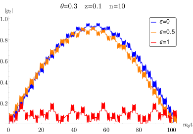
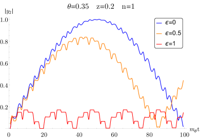
Figure 6: The oscillating behaviour of $|y_{2}(t)|$ in resonance (2.43) ($\epsilon=0$) and that excluding all regions near the points $M_{\rm eff}(t)=0$ (A.15) ($\epsilon=0.5,1$) for two sets of parameters.

We confirm that the regions $|z+\sin m_{\phi}t|\ll\left(\frac{\displaystyle m_{\phi}}{\displaystyle\beta}\right)^{1/3}$ (A.12) really give only sub-dominant contributions to the transition probability as argued above. We also varified that our method in case $\epsilon\leq 0.2$ enterily reproduces the resonant behaviour ($\epsilon=0$) but we do not show it in Fig. 6 for a clear representation. For $\epsilon=1$ we do not find any significant amplification of the amplitude $|y_{2}(t)|$. It justifies our statement that non-trivial dynamic in system (2.28) manifests itself mainly at (A.15).

Once the relevant mass scale related to the resonance behaviour (A.15) is found one can verify our primordial assumptions (A.1), (A.2). We assume that the error budget of our framework (2.28) in the resonance is insignificantly small if (A.1) and (A.2) are violated far beyond the region where resonance reveals itself (A.15). Consequently, we require

$$2\theta z\ll\left(\frac{m_{\phi}}{\beta}\right)^{1/3},\qquad\text{and}\qquad\left(\theta z\frac{m_{\phi}}{2\beta}\right)^{1/4}\ll\left(\frac{m_{\phi}}{\beta}\right)^{1/3}.$$ (A.16)

Finally, our framework (2.28) can be applied to describe neutrino oscillations in resonance (2.43) only if (A.16), i.e.,

$$\begin{split}2\theta z\ll&\left(\frac{m_{\phi}}{\beta}\right)^{1/3}\approx\frac{1}{n^{1/3}}\end{split}$$ (A.17)

is addressed where in last equality we used (2.32).

For the reasonable values of oscillations parameters (2.32) and not too large $n$ the condition (A.17) is always fulfilled. This justifies the applicability of simplified oscillation framework (2.28) used in the numerical analyses of Sec. 2.

References

- [1] F. Bezrukov, A. Chudaykin and D. Gorbunov, Hiding an elephant: heavy sterile neutrino with large mixing angle does not contradict cosmology, JCAP 1706 (2017) 051, [1705.02184].
- [2] F. Bezrukov, A. Chudaykin and D. Gorbunov, Induced resonance makes light sterile neutrino Dark Matter cool, 1809.09123.
- [3] G. Bertone and D. Hooper, History of dark matter, Rev. Mod. Phys. 90 (2018) 045002, [1605.04909].
- [4] D. S. Gorbunov, Sterile neutrinos and their role in particle physics and cosmology, Phys. Usp. 57 (2014) 503–511.
- [5] S. Bilenky, Neutrino oscillations: From a historical perspective to the present status, Nucl. Phys. B908 (2016) 2–13, [1602.00170].
- [6] M. Drewes et al., A White Paper on keV Sterile Neutrino Dark Matter, JCAP 1701 (2017) 025, [1602.04816].
- [7] K. N. Abazajian, Sterile neutrinos in cosmology, Phys. Rept. 711-712 (2017) 1–28, [1705.01837].
- [8] A. Schneider, Astrophysical constraints on resonantly produced sterile neutrino dark matter, JCAP 1604 (2016) 059, [1601.07553].
- [9] A. Boyarsky, O. Ruchayskiy and D. Iakubovskyi, A Lower bound on the mass of Dark Matter particles, JCAP 0903 (2009) 005, [0808.3902].
- [10] D. Gorbunov, A. Khmelnitsky and V. Rubakov, Constraining sterile neutrino dark matter by phase-space density observations, JCAP 0810 (2008) 041, [0808.3910].
- [11] B. M. Roach, K. C. Y. Ng, K. Perez, J. F. Beacom, S. Horiuchi, R. Krivonos et al., NuSTAR Tests of Sterile-Neutrino Dark Matter: New Galactic Bulge Observations and Combined Impact, 1908.09037.
- [12] S. Dodelson and L. M. Widrow, Sterile-neutrinos as dark matter, Phys. Rev. Lett. 72 (1994) 17–20, [hep-ph/9303287].
- [13] X.-D. Shi and G. M. Fuller, A New dark matter candidate: Nonthermal sterile neutrinos, Phys. Rev. Lett. 82 (1999) 2832–2835, [astro-ph/9810076].
- [14] Y. Farzan, Ultra-light scalar saving the 3 + 1 neutrino scheme from the cosmological bounds, Phys. Lett. B797 (2019) 134911, [1907.04271].
- [15] J. M. Cline, Viable secret neutrino interactions with ultralight dark matter, 1908.02278.
- [16] M. Pavlinsky et al., Spectrum-Roentgen-Gamma astrophysical mission, Proc. SPIE Int. Soc. Opt. Eng. 7011 (2008) 70110H.
- [17] eROSITA collaboration, A. Merloni et al., eROSITA Science Book: Mapping the Structure of the Energetic Universe, 1209.3114.
- [18] G. D. Pusch, NEUTRON OSCILLATIONS IN A PERIODICALLY VARYING MAGNETIC FIELD, Nuovo Cim. A74 (1983) 149.
- [19] A. M. Egorov, A. E. Lobanov and A. I. Studenikin, Neutrino oscillations in electromagnetic fields, Phys. Lett. B491 (2000) 137–142, [hep-ph/9910476].
- [20] M. Dvornikov and A. Studenikin, Parametric resonance of neutrino oscillations in electromagnetic wave, in New worlds in astroparticle physics. Proceedings, 3rd International Workshop, Faro, Portugal, September 1-3, 2000, pp. 126–131, 2000. hep-ph/0102099. DOI.
- [21] M. Dvornikov, Neutrino spin-flavor oscillations in frequently varying external fields, Phys. Atom. Nucl. 70 (2007) 342–348, [hep-ph/0410152].
- [22] A. Erdelyi, Asymptotic Expansions.
- [23] K. Abazajian, G. M. Fuller and M. Patel, Sterile neutrino hot, warm, and cold dark matter, Phys. Rev. D64 (2001) 023501, [astro-ph/0101524].
- [24] G. Sigl and G. Raffelt, General kinetic description of relativistic mixed neutrinos, Nucl. Phys. B406 (1993) 423–451.
- [25] M. Shaposhnikov and I. Tkachev, The nuMSM, inflation, and dark matter, Phys. Lett. B639 (2006) 414–417, [hep-ph/0604236].
- [26] A. Kusenko, Sterile neutrinos, dark matter, and the pulsar velocities in models with a Higgs singlet, Phys. Rev. Lett. 97 (2006) 241301, [hep-ph/0609081].
- [27] K. Petraki and A. Kusenko, Dark-matter sterile neutrinos in models with a gauge singlet in the Higgs sector, Phys. Rev. D77 (2008) 065014, [0711.4646].
- [28] D. Malyshev, A. Neronov and D. Eckert, Constraints on keV line emission from stacked observations of dwarf spheroidal galaxies, Phys. Rev. D90 (2014) 103506, [1408.3531].
- [29] S. Horiuchi, P. J. Humphrey, J. Onorbe, K. N. Abazajian, M. Kaplinghat and S. Garrison-Kimmel, Sterile neutrino dark matter bounds from galaxies of the Local Group, Phys. Rev. D89 (2014) 025017, [1311.0282].
- [30] M. Laine and M. Shaposhnikov, Sterile neutrino dark matter as a consequence of nuMSM-induced lepton asymmetry, JCAP 0806 (2008) 031, [0804.4543].
- [31] F. Bezrukov, H. Hettmansperger and M. Lindner, keV sterile neutrino Dark Matter in gauge extensions of the Standard Model, Phys. Rev. D81 (2010) 085032, [0912.4415].
- [32] A. Kusenko, F. Takahashi and T. T. Yanagida, Dark Matter from Split Seesaw, Phys. Lett. B693 (2010) 144–148, [1006.1731].
- [33] V. K. Romanko, The course of differential equations and the calculus of variations.