Topological Properties of Secure Wireless Sensor Networks under the $q$-Composite Key Predistribution Scheme with Unreliable Links

Abstract

Security is an important issue in wireless sensor networks (WSNs), which are often deployed in hostile environments. The $q$-composite key predistribution scheme has been recognized as a suitable approach to secure WSNs. Although the $q$-composite scheme has received much attention in the literature, there is still a lack of rigorous analysis for secure WSNs operating under the $q$-composite scheme in consideration of the unreliability of links. One main difficulty lies in analyzing the network topology whose links are not independent. Wireless links can be unreliable in practice due to the presence of physical barriers between sensors or because of harsh environmental conditions severely impairing communications. In this paper, we resolve the difficult challenge and investigate topological properties related to node degree in WSNs operating under the $q$-composite scheme with unreliable communication links modeled as independent on/off channels. Specifically, we derive the asymptotically exact probability for the property of minimum degree being at least $k$, present the asymptotic probability distribution for the minimum degree, and demonstrate that the number of nodes with an arbitrary degree is in distribution asymptotically equivalent to a Poisson random variable. We further use the theoretical results to provide useful design guidelines for secure WSNs. Experimental results also confirm the validity of our analytical findings.

I Introduction

Wireless sensor networks (WSNs) enable a broad range of applications including military surveillance, home automation, and patient monitoring [1]. In many scenarios, since WSNs are deployed in adversarial environments, security becomes an important issue. To this end, key predistribution has been recognized as a typical solution to secure WSNs [2]. The idea is to randomly assign cryptographic keys to sensors before network deployment. Various key predistribution schemes have been studied in the literature [3, 4, 5, 6, 1, 2, 7, 8, 9, 10, 11, 12, 13].

The $q$-composite key predistribution scheme proposed by Chan et al. [1] as an extension of the Eschenauer-Gligor scheme [2] (the $q$-composite scheme in the case of $q=1$) has received much interest [10, 11, 12, 13, 14, 15, 16, 17] since its introduction. The $q$-composite scheme when $q\geq 2$ outperforms the Eschenauer-Gligor scheme in terms of the strength against small-scale network capture attacks while trading off increased vulnerability in the face of large-scale attacks.

The $q$-composite scheme [1] works as follows. For a WSN with $n$ sensors, prior to deployment, each sensor is independently assigned $K_{n}$ different keys which are selected uniformly at random from a pool of $P_{n}$ keys, where $K_{n}$ and $P_{n}$ are both functions of $n$, with $K_{n}\leq P_{n}$. Then two sensors establish a link in between after deployment if and only if they share at least $q$ keys and the physical link constraint between them is satisfied. Examples of physical link constraints include the reliability of the transmission channel [3, 5] and the requirement that the distance between two sensors should be close enough for communication [16].

Communication links between sensor nodes may not be available due to the presence of physical barriers between nodes or because of harsh environmental conditions severely impairing transmission. To represent unreliable links, we use the on/off channel model where each link is either on (i.e., active) with probability $p_{n}$ or off (i.e., inactive) with probability $(1-p_{n})$, where $p_{n}$ is a function of $n$ for generality.

In addition to link failure, sensor nodes are also prone to failure in WSNs deployed in hostile environments. To ensure reliability against the failure of sensors, we study the property of minimum degree being at least $k$ so that each sensor is directly connected to at least $k$ other sensors. This means that a sensor may still be connected to a sufficient number of sensors even if some neighbors fail. Note that the degree of a node $v$ is the number of nodes having links with $v$; and the minimum (node) degree of a network is the least among the degrees of all nodes. Another related graph property is $k$-connectivity, which is stronger than the property of minimum degree being at least $k$. A network (or a graph) is said to be $k$-connected if it remains connected despite the deletion of any $(k-1)$ nodes [18, 19]; a network is simply deemed connected if it is $1$-connected. Hence, $k$-connectivity provides a guarantee of network reliability against the failure of $(k-1)$ sensors due to adversarial attacks, battery depletion, harsh environmental conditions, etc.

In view of the above, we investigate topological properties related to node degree in WSNs employing the $q$-composite key predistribution scheme under the on/off channel model as the physical link constraint comprising independent channels which are either on or off. Specifically, we derive the asymptotically exact probabilities for the property of minimum degree being at least $k$, establish the asymptotic probability distribution for the minimum degree, and show that the number of nodes with an arbitrary degree is in distribution asymptotically equivalent to a Poisson random variable. Our results are useful for designing secure WSNs under link and node failure.

We summarize our contributions in the following two subsections. We first present our results on node degree for a secure WSN employing the $q$-composite key predistribution scheme under the on/off channel model. Then we use the results to provide useful design guidelines for secure WSNs.

I-A Results

For $\mathbb{G}_{q}$ denoting a secure sensor network with the $q$-composite key predistribution scheme under the on/off channel model, we present several results related to node degree, by considering the conditions on $p_{e,q}$, which denotes the probability of a secure link between two sensors. The secure link probability $p_{e,q}$ is given by $p_{e,q}=p_{n}\cdot\left[1-\sum_{u=0}^{q-1}\frac{\binom{K_{n}}{u}\binom{P_{n}-K_{n}}{K_{n}-u}}{\binom{P_{n}}{K_{n}}}\right]$, as shown in Equation (8) on Page 8 later.

For the network $\mathbb{G}_{q}$, we now present the results, which are further elaborated in Section III-A.

• First, we derive the asymptotically exact probabilities for the property of minimum degree being at least $k$. Specifically, if $p_{e,q}=\frac{\ln n+{(k-1)}\ln\ln n+{\alpha_{n}}}{n}$ for a constant integer $k\geq 1$ and a sequence $\alpha_{n}$ satisfying $\lim_{n\to\infty}\alpha_{n}\in[-\infty,\infty]$, then the probability that $\mathbb{G}_{q}$ has a minimum degree at least $k$ converges to $e^{-\frac{e^{-\lim_{n\to\infty}\alpha_{n}}}{(k-1)!}}$, which equals (i) $e^{-\frac{e^{-\alpha^{*}}}{(k-1)!}}$ if $\lim_{n\to\infty}\alpha_{n}=\alpha^{*}\in(-\infty,\infty)$, (ii) $1$ if $\lim_{n\to\infty}\alpha_{n}=\infty$, and (iii) $0$ if $\lim_{n\to\infty}\alpha_{n}=-\infty$.

• We extend the above result to provide the asymptotic probability distribution for the minimum degree. Specifically, when $\alpha_{n}$ above can be written as $\alpha_{n}=b\ln\ln n+\beta_{n}$ for a constant integer $b$ and a sequence $\beta_{n}$ satisfying $-1<\liminf_{n\to\infty}\frac{\beta_{n}}{\ln\ln n}\leq\limsup_{n\to\infty}\frac{\beta_{n}}{\ln\ln n}<1$ (i.e., $c_{1}\ln\ln n\leq\beta_{n}\leq c_{2}\ln\ln n$ for constants $-1<c_{1}\leq c_{2}<1$), we have the following:

  • if $k+b\geq 1$ and $\lim_{n\to\infty}\beta_{n}\in[-\infty,\infty]$, then the minimum degree of $\mathbb{G}_{q}$ in the asymptotic sense equals (i) $k+b$ with probability $e^{-\frac{e^{-\lim_{n\to\infty}\beta_{n}}}{(k-1)!}}$, (ii) $k+b-1$ with probability $1-e^{-\frac{e^{-\lim_{n\to\infty}\beta_{n}}}{(k-1)!}}$, and (iii) other values with probability $0$;

  • if $k+b\leq 0$, then the minimum degree of $\mathbb{G}_{q}$ in the asymptotic sense equals $0$ with probability $1$.

• Our results on minimum degree are obtained by analyzing the number of nodes with a fixed degree. Specifically, we show that for a non-negative constant integer $h$, the number of nodes in $\mathbb{G}_{q}$ with degree $h$ is in distribution asymptotically equivalent to a Poisson random variable with mean $n(h!)^{-1}(np_{e,q})^{h}e^{-np_{e,q}}$.

I-B Design guidelines for secure sensor networks

Based on the above results, for $\mathbb{G}_{q}$ denoting a secure sensor network employing the $q$-composite key predistribution scheme under the on/off channel model, we obtain several guidelines below for choosing parameters to ensure that the network $\mathbb{G}_{q}$ has certain minimum node degree. The guidelines are given by enforcing conditions on $p_{e,q}$, the probability of a secure link between two sensors. Note that $p_{e,q}=p_{n}\cdot\left[1-\sum_{u=0}^{q-1}\frac{\binom{K_{n}}{u}\binom{P_{n}-K_{n}}{K_{n}-u}}{\binom{P_{n}}{K_{n}}}\right]$; see Equation (8) later.

For the network $\mathbb{G}_{q}$, we now present the design guidelines, which are further explained in Section III-B.

• First, to ensure that the network $\mathbb{G}_{q}$ has a minimum degree no less than $k$ (i.e., to ensure that each sensor is directly connected to at least $k$ other sensors), we can choose network parameters to have

  $$p_{e,q}\geq\frac{\ln n+{(k+c_{1}-1)}\ln\ln n}{n}\text{ for a constant $c_{1}>0$,}$$ (1)

  where the positive constant $c_{1}$ can be arbitrarily small.

• Second, to guarantee that the network $\mathbb{G}_{q}$ has a minimum degree at least $k$ with probability no less than $\rho$, we choose parameters to have

  $$p_{e,q}\geq\frac{\ln n+{(k-1)}\ln\ln n-\ln[(k-1)!\ln\frac{1}{\rho}]}{n}.$$ (2)

• Third, to ensure that the network $\mathbb{G}_{q}$ has a minimum degree being $k$ exactly, we can choose network parameters to have

  $$p_{e,q}=\frac{\ln n+{(k+c_{2}-1)}\ln\ln n}{n}\text{ for a constant $0<c_{2}<1$,}$$ (3)

  where the positive constant $c_{2}$ can be arbitrarily small.

I-C Roadmap

We organize the rest of the paper as follows. Section II describes the system model in detail. Afterwards, we elaborate and discuss the results in Section III. In Section IV, we prove Theorems 1 and 2 using Theorem 3. In Section V, we detail the steps of establishing Theorem 3 through Lemma 1. Section VI provides the proof of Lemma 1 by the help of Propositions 1 and 2, which are proved in Sections VII and VIII, respectively. Subsequently, we present experiments in Section IX to confirm our analytical results. Section X is devoted to relevant results in the literature. Next, we conclude the paper and identify future research directions in Section XI, followed by the Appendix.

II System Model

Our approach to the analysis is to explore the induced random graph models of the WSNs. As will be clear soon, the graph modeling a WSN under $q$-composite scheme and the on/off channel model is an intersection of two graphs belonging to different kinds, which renders the analysis challenging due to the intertwining of the two distinct types of random graphs [5, 20].

We elaborate the graph modeling of a WSN with $n$ sensors, which employs the $q$-composite key predistribution scheme and works under the on/off channel model. We consider a node set $\mathcal{V}=\{v_{1},v_{2},\ldots,v_{n}\}$ to represent the $n$ sensors (a sensor is also referred to as a node). For each node $v_{i}\in\mathcal{V}$, the set of its $K_{n}$ different keys is denoted by $S_{i}$, which is uniformly distributed among all $K_{n}$-size subsets of a key pool of $P_{n}$ keys, and is referred to as the key ring of node $v_{i}$.

The $q$-composite key predistribution scheme is modeled by a graph denoted by $G_{q}(n,K_{n},P_{n})$, which is defined on the vertex set $\mathcal{V}$ such that any two different nodes $v_{i}$ and $v_{j}$ sharing at least $q$ keys (such event is denoted by $\Gamma_{ij}$) have an edge in between. With $S_{ij}:=S_{i}\cap S_{j}$, event $\Gamma_{ij}$ equals $\big{[}|S_{ij}|\geq q\big{]}$, where $|A|$ with $A$ as a set means the cardinality of $A$.

As discussed, under the on/off channel model, each node-to-node channel independently has probability $p_{n}$ of being on and probability $(1-p_{n})$ of being off, where $p_{n}$ is a function of $n$. Denoting by ${B}_{ij}$ the event that the channel between distinct nodes $v_{i}$ and $v_{j}$ is on, we have ${\mathbb{P}}\left[{C_{ij}}\right]=p_{n}$, where $\mathbb{P}[\mathcal{E}]$ denotes the probability that event $\mathcal{E}$ happens, throughout the paper. The on/off channel model is represented by an Erdős-Rényi graph $G(n,p_{n})$ [21] defined on the node set $\mathcal{V}$ such that $v_{i}$ and $v_{j}$ have an edge in between if event $C_{ij}$ happens.

Finally, we denote by $\mathbb{G}_{q}(n,K_{n},P_{n},p_{n})$ the underlying graph of the $n$-node WSN operating under the $q$-composite key predistribution scheme and the on/off channel model. We often write $\mathbb{G}_{q}$ rather than $\mathbb{G}_{q}(n,K_{n},P_{n},p_{n})$ for notation brevity. Graph $\mathbb{G}_{q}$ is defined on the node set $\mathcal{V}$ such that there exists an edge between nodes $v_{i}$ and $v_{j}$ if events $\Gamma_{ij}$ and $C_{ij}$ happen at the same time. We set event $E_{ij}:=\Gamma_{ij}\cap C_{ij}$ and also write $E_{ij}$ as $E_{v_{i}v_{j}}$ when necessary. It is clear that $\mathbb{G}_{q}$ can be seen as the intersection of $G_{q}(n,K_{n},P_{n})$ and $G(n,p_{n})$, meaning

$$\mathbb{G}_{q}=G_{q}(n,K_{n},P_{n})\cap G(n,p_{n}).$$ (4)

We define $p_{s,q}$ as the probability that two different nodes share at least $q$ keys and $p_{e,q}$ as the probability that two distinct nodes have a link in between, where the subscripts “s” and “e” are short for “secure” and “edge”, respectively. $p_{s,q}$ and $p_{e,q}$ both rely on $K_{n},P_{n}$ and $q$, while $p_{e,q}$ also depends on $p_{n}$. Under $P_{n}\geq 2K_{n}$, we determine $p_{s,q}$ through

$$p_{s,q}=\mathbb{P}[\Gamma_{ij}] =\sum_{u=q}^{K_{n}}\mathbb{P}[|S_{i}\cap S_{j}|=u]$$

$$=1-\sum_{u=0}^{q-1}\mathbb{P}[|S_{i}\cap S_{j}|=u],$$ (5)

where

$$\mathbb{P}[|S_{i}\cap S_{j}|=u]=\frac{\binom{K_{n}}{u}\binom{P_{n}-K_{n}}{K_{n}-u}}{\binom{P_{n}}{K_{n}}},\textrm{ for }u=0,1,\ldots,K_{n},$$ (6)

since $S_{i}$ and $S_{j}$ are independently and uniformly selected from all $K_{n}$-size subsets of a key pool with size $P_{n}$. Then by the independence of events ${C}_{ij}$ and $\Gamma_{ij}$, we obtain

$${p_{e,q}} =\mathbb{P}[E_{ij}]=\mathbb{P}[{C}_{ij}]\cdot\mathbb{P}[\Gamma_{ij}]=p_{n}\cdot p_{s,q}.$$ (7)

Summarizing (5) (6) (7), we derive that under $P_{n}\geq 2K_{n}$, the link probability $p_{e,q}$ is given by

$$p_{e,q} =p_{n}\cdot\left[1-\sum_{u=0}^{q-1}\frac{\binom{K_{n}}{u}\binom{P_{n}-K_{n}}{K_{n}-u}}{\binom{P_{n}}{K_{n}}}\right].$$ (8)

III The Results and Discussion

We present and discuss the results in this section. Throughout the paper, $q$ is a positive integer and does not scale with $n$; $\mathbb{N}_{0}$ stands for the set of all positive integers; $\mathbb{R}$ is the set of all real numbers; $e$ is the base of the natural logarithm function, $\ln$; and the floor function $\lfloor x\rfloor$ is the largest integer not greater than $x$. We consider $e^{\infty}=\infty$ and $e^{-\infty}=0$. The term “for all $n$ sufficiently large” means “for any $n\geq N$, where $N\in\mathbb{N}_{0}$ is selected appropriately”. As already mentioned, all asymptotic statements are understood with $n\to\infty$, and we use the standard asymptotic notation $o(\cdot),O(\cdot),\omega(\cdot),\Omega(\cdot),\Theta(\cdot),\sim$; see [3, Page 2-Footnote 1]. In particular, for two positive sequences $f_{n}$ and $g_{n}$, $f_{n}\sim g_{n}$ signifies $\lim_{n\to\infty}\frac{{f_{n}}}{g_{n}}=1$; namely, $f_{n}$ and $g_{n}$ are asymptotically equivalent.

III-A The Results of Graph $\mathbb{G}_{q}$

We now present the results of graph $\mathbb{G}_{q}$ below.

Theorem 1 provides the probability of minimum degree being at least $k$ in $\mathbb{G}_{q}$.

Theorem 1 (Minimum degree in graph $\mathbb{G}_{q}$).

For graph $\mathbb{G}_{q}$ with $K_{n}=\omega(1)$ and $\frac{{K_{n}}^{2}}{P_{n}}=o(1)$, if there exist a constant integer $k\geq 1$ and a sequence $\alpha_{n}$ satisfying $\lim\limits_{n\to\infty}\alpha_{n}\in[-\infty,\infty]$ such that

$$p_{e,q}=\frac{\ln n+{(k-1)}\ln\ln n+{\alpha_{n}}}{n},$$ (9)

then with $\delta$ denoting the minimum degree of $\mathbb{G}_{q}$, we have

$$\lim\limits_{n\to\infty}{\mathbb{P}}\left[{\delta\geq k}\right]$$

$$= e^{-\frac{e^{-\alpha^{*}}}{(k-1)!}}, \lim\limits_{n\to\infty}\alpha_{n}=\alpha^{*}\in(-\infty,\infty)$$ if , (10a)

$$= 1, \lim\limits_{n\to\infty}\alpha_{n}=\infty$$ if , (10b)

$$= 0, \lim\limits_{n\to\infty}\alpha_{n}=-\infty$$ if . (10c)

Remark 1.

The results (10a) (10b) (10c) can be compactly summarized as $\lim_{n\to\infty}{\mathbb{P}}\left[{\delta\geq k}\right]=e^{-\frac{e^{-\lim_{n\to\infty}\alpha_{n}}}{(k-1)!}}$.

Interpreting Theorem 1. Theorem 1 for graph $\mathbb{G}_{q}$ presents the asymptotically exact probability and a zero–one law for the event that $\mathbb{G}_{q}$ has a minimum degree no less than $k$, where a zero–one law means that the probability of a graph having a certain property asymptotically converges to $0$ under some conditions and to $1$ under some other conditions. To establish Theorem 1, we explain the basic ideas in Section III-C, and more technical details in Section IV.

While Theorem 1 above is for the property of minimum degree being at least some value, we now present Theorem 2 below, which gives a more fine-grained result to provide the asymptotic probability distribution for the minimum degree.

Theorem 2 (Minimum degree in graph $\mathbb{G}_{q}$: More fine-grained results compared with Theorem 1).

Under the conditions of Theorem 1, if $\alpha_{n}$ in Equation (9) can be written as

$$\alpha_{n}=b\ln\ln n+\beta_{n}$$ (11)

for a constant integer $b$ and a sequence $\beta_{n}$ satisfying

$$-1<\liminf_{n\to\infty}\frac{\beta_{n}}{\ln\ln n}\leq\limsup_{n\to\infty}\frac{\beta_{n}}{\ln\ln n}<1,$$ (12)

then with $\delta$ denoting the minimum degree of $\mathbb{G}_{q}$, the properties ①–④ below follow:

• for ${k+b\leq 0}$ (which implies $b\leq-k\leq-1$ given $k\geq 1$), we have

  $$\lim\limits_{n\to\infty}{\mathbb{P}}\left[{\delta=0}\right]=1,$$ (13a)

  $$\lim\limits_{n\to\infty}{\mathbb{P}}\left[{\delta>0}\right]=0;$$ (13b)

• and for ${k+b\geq 1}$ (i.e., $b\geq 1-k$), we obtain properties ②–⑤:

• $\lim\limits_{n\to\infty}{\mathbb{P}}\left[{(\delta=k+b)\text{ or }(\delta=k+b-1)}\right]=1$;

• if $\lim\limits_{n\to\infty}\beta_{n}=\beta^{*}\in(-\infty,\infty)$, then

  $$\lim\limits_{n\to\infty}{\mathbb{P}}\left[{\delta=k+b}\right]=e^{-\frac{e^{-\beta^{*}}}{(k+b-1)!}},$$ (14a)

  $$\lim\limits_{n\to\infty}{\mathbb{P}}\left[{\delta=k+b-1}\right]=1-e^{-\frac{e^{-\beta^{*}}}{(k+b-1)!}};$$ (14b)

• if $\lim\limits_{n\to\infty}\beta_{n}=\infty$, then

  $$\lim\limits_{n\to\infty}{\mathbb{P}}\left[{\delta=k+b}\right]=1,$$ (15a)

  $$\lim\limits_{n\to\infty}{\mathbb{P}}\left[{\delta\neq k+b}\right]=0;$$ (15b)

• if $\lim\limits_{n\to\infty}\beta_{n}=-\infty$, then

  $$\lim\limits_{n\to\infty}{\mathbb{P}}\left[{\delta=k+b-1}\right]=1,$$ (16a)

  $$\lim\limits_{n\to\infty}{\mathbb{P}}\left[{\delta\neq k+b-1}\right]=0.$$ (16b)

Remark 2.

The above results ③–⑤ for $k+b\geq 1$ and $\lim_{n\to\infty}\beta_{n}\in[-\infty,\infty]$ can be compactly summarized as that the minimum degree of $\mathbb{G}_{q}$ in the asymptotic sense equals (i) $k+b$ with probability $e^{-\frac{e^{-\lim_{n\to\infty}\beta_{n}}}{(k-1)!}}$, (ii) $k+b-1$ with probability $1-e^{-\frac{e^{-\lim_{n\to\infty}\beta_{n}}}{(k-1)!}}$, and (iii) other values with probability $0$, while results ① says that if $k+b\leq 0$, then the minimum degree of $\mathbb{G}_{q}$ in the asymptotic sense equals $0$ with probability $1$.

Interpreting Theorem 2. Theorem 2 presents the asymptotic probability distribution for the minimum degree. We explain that Theorem 2 is more fine-grained than Theorem 1. We discuss first Theorem 2’s result ① and then its results ②–⑤.

• In result ① above, $b\leq-k\leq-1$ follows from $k+b\leq 0$ and $k\geq 1$. Using $b\leq-1$ and (12) in (11), we have $\lim_{n\to\infty}\alpha_{n}=-\infty$, so we use (10c) of Theorem 1 to obtain $\delta<k$ almost surely (an event happens almost surely if its probability converges $1$ as $n\to\infty$), where $\delta$ denotes the minimum degree of $\mathbb{G}_{q}$. For comparison, (13a) of Theorem 2 presents the stronger result that $\delta=0$ almost surely.

• In the above results ②–⑤ where ${k+b\geq 1}$ holds (i.e., $b\geq 1-k$) , we derive from (11) and (12) that

  $$\lim\limits_{n\to\infty}\alpha_{n}= \infty, b\geq 1$$ if , (17a)

  $$\lim\limits_{n\to\infty}\alpha_{n}= \beta^{*}, b=0 \lim\limits_{n\to\infty}\beta_{n}=\beta^{*}\in(-\infty,\infty)$$ if and , (17b)

  $$\lim\limits_{n\to\infty}\alpha_{n}= \infty, b=0 \lim\limits_{n\to\infty}\beta_{n}=\infty$$ if and , (17c)

  $$\lim\limits_{n\to\infty}\alpha_{n}= -\infty, b=0 \lim\limits_{n\to\infty}\beta_{n}=-\infty$$ if and , (17d)

  $$\lim\limits_{n\to\infty}\alpha_{n}= -\infty, b\leq-1$$ if . (17e)

  Below we discuss (17a)–(17e), respectively.

  • For (17a) above, (10b) of Theorem 1 says $\delta\geq k$ almost surely, while ② of Theorem 2 presents the stronger result that $\delta$ equals $k+b$ or $k+b-1$ almost surely (note $b\geq 1$ in (17a)).

  • For (17b) above, (10a) of Theorem 1 says $\delta\geq k$ with probability $e^{-\frac{e^{-\beta^{*}}}{(k+b-1)!}}$ asymptotically, while ③ of Theorem 2 presents the stronger result that $\delta$ equals $k$ (note $b=0$ in (17b) here) with probability $e^{-\frac{e^{-\beta^{*}}}{(k+b-1)!}}$ asymptotically, and equals $k-1$ with probability $1-e^{-\frac{e^{-\beta^{*}}}{(k+b-1)!}}$ asymptotically (note $b=0$ in (17b) here).

  • For (17c) above, (10b) of Theorem 1 says $\delta\geq k$ almost surely, while ④ of Theorem 2 presents the stronger result that $\delta=k$ almost surely (note $b=0$ in (17c) here).

  • For (17d) above, (10c) of Theorem 1 says $\delta<k$ almost surely, while ⑤ of Theorem 2 presents the stronger result that $\delta=k-1$ almost surely (note $b=0$ in (17d) here).

  • For (17e) above, (10c) of Theorem 1 says $\delta<k$ almost surely, while ② of Theorem 2 presents the stronger result that $\delta$ equals $k+b$ or $k+b-1$ almost surely (note $b\leq-1$ in (17e)).

Summarizing the above, compared with Theorem 1, Theorem 2 presents a more fine-grained result for minimum degree in $\mathbb{G}_{q}$.

To prove Theorem 2, we provide the basic ideas in Section III-C, and more technical details in Section IV.

Theorems 1 and 2 above are for the property of minimum degree being at least $k$. We now consider a stronger graph/network property, namely $k$-connectivity.

Extension to $k$-connectivity. We can extend Theorem 1 to obtain the probability of $k$-connectivity in $\mathbb{G}_{q}$. Specifically, we can replace $\lim_{n\to\infty}{\mathbb{P}}\left[{\delta\geq k}\right]$ by $\lim_{n\to\infty}{\mathbb{P}}\left[{\text{$\mathbb{G}_{q}$ is $k$-connected.}}\right]$, at the cost of replacing $K_{n}=\omega(1)$ and $\frac{{K_{n}}^{2}}{P_{n}}=o(1)$ by a stronger condition set $\frac{{K_{n}}^{2}}{P_{n}}=o\left(\frac{1}{\ln n}\right)$, $\frac{K_{n}}{P_{n}}=o\left(\frac{1}{n\ln n}\right)$ and $K_{n}=\Omega(n^{\epsilon})$ for a positive constant $\epsilon$. Due to space limitation, we present the proof in the full version [22].

III-B Design guidelines for secure sensor networks

Based on the above results, now we provide several design guidelines of secure sensor networks for achieving certain strength of minimum degree.

• First, to ensure that $\mathbb{G}_{q}$ has a minimum degree no less than $k$, we can choose network parameters to set

  $$p_{e,q}\geq\frac{\ln n+{(k+c_{1}-1)}\ln\ln n}{n}\text{ for a constant $c_{1}>0$,}$$ (18)

  where the positive constant $c_{1}$ can be arbitrarily small. To see this, since (18) implies that $\alpha_{n}$ defined by (9) (i.e., $p_{e,q}=\frac{\ln n+{(k-1)}\ln\ln n+{\alpha_{n}}}{n}$) satisfies $\lim_{n\to\infty}\alpha_{n}=\infty$, we use Theorem 1 to have ${\mathbb{P}}\left[{\text{$\mathbb{G}_{q}$ has a minimum degree at least $k$.}}\right]=1$.

• Second, to guarantee that $\mathbb{G}_{q}$ has a minimum degree at least $k$ with probability no less than $\rho$, we choose parameters to ensure

  $$p_{e,q}\geq\frac{\ln n+{(k-1)}\ln\ln n-\ln[(k-1)!\ln\frac{1}{\rho}]}{n}.$$ (19)

  To see this, since (19) implies that $\alpha_{n}$ defined by (9) (i.e., $p_{e,q}=\frac{\ln n+{(k-1)}\ln\ln n+{\alpha_{n}}}{n}$) satisfies $\alpha_{n}\geq-\ln[(k-1)!\ln\frac{1}{\rho}]$, we use Theorem 1 to obtain ${\mathbb{P}}\left[{\text{$\mathbb{G}_{q}$ has a minimum degree at least $k$.}}\right]\geq e^{-\frac{e^{\ln[(k-1)!\ln\frac{1}{\rho}]}}{(k-1)!}}=\rho$.

• Third, to ensure that $\mathbb{G}_{q}$ has a minimum degree being $k$ exactly, we can choose network parameters to have

  $$p_{e,q}=\frac{\ln n+{(k+c_{2}-1)}\ln\ln n}{n}\text{ for a constant $0<c_{2}<1$,}$$ (20)

  where the positive constant $c_{2}$ can be arbitrarily small. To see this, (20) implies that $\alpha_{n}$ defined by (9) (i.e., $p_{e,q}=\frac{\ln n+{(k-1)}\ln\ln n+{\alpha_{n}}}{n}$) equals $c_{2}\ln\ln n$, so $b$ in (11) is $0$ with $\beta_{n}$ satisfying (11) and $\lim_{n\to\infty}\beta_{n}=\infty$. Then we use Theorem 1-Result ④ to obtain ${\mathbb{P}}\left[{\text{Minimum degree of $\mathbb{G}_{q}$ equals $k$ {exactly}.}}\right]=1$.

III-C Basic Ideas to Establish Theorems 1 and 2

We establish Theorems 1 and 2 for minimum degree in graph $\mathbb{G}_{q}$ by analyzing the number of nodes with a fixed degree, for which we present Theorem 3 below. The details of using Theorem 3 to prove Theorems 1 and 2 are given in Section IV.

Theorem 3 (Possion distribution for number of nodes with a fixed degree in graph $\mathbb{G}_{q}$).

For graph $\mathbb{G}_{q}$ with $K_{n}=\omega(1)$ and $\frac{{K_{n}}^{2}}{P_{n}}=o(1)$, if

$$p_{e,q} =\frac{\ln n\pm O(\ln\ln n)}{n}$$ (21)

(i.e., $\frac{np_{e,q}-\ln n}{\ln\ln n}$ is bounded), then for a non-negative constant integer $h$, the number of nodes in $\mathbb{G}_{q}$ with degree $h$ is in distribution asymptotically equivalent to a Poisson random variable with mean $\lambda_{n,h}:=n(h!)^{-1}(np_{e,q})^{h}e^{-np_{e,q}}$; i.e., as $n\to\infty$,

$${\mathbb{P}}\left[{\begin{array}[]{l}\text{The number of nodes in $\mathbb{G}_{q}$}\\ \text{with degree $h$ equals $\ell$.}\end{array}}\right]\Big{/}\Big{[}(\ell!)^{-1}{\lambda_{n,h}}^{\ell}e^{-\lambda_{n,h}}\Big{]}\to 1,$$ (24)

                                           for $$\ell=0,1,\ldots$$ (25)

Interpreting Theorem 3. Theorem 3 for graph $\mathbb{G}_{q}$ shows that the number of nodes with a fixed degree follows a Poisson distribution asymptotically.

III-D The Practicality of the Theorem Conditions

We check the practicality of the conditions in Theorem 1: $K_{n}=\omega(1)$ and $\frac{{K_{n}}^{2}}{P_{n}}=o(1)$. The condition $K_{n}=\omega(1)$ means that the key ring size $K_{n}$ on a sensor grows with the number $n$ of sensors and thus it follows trivially in secure wireless sensor networks [23, 10, 24]. For $k$-connectivity, the condition on $K_{n}$ (i.e., $K_{n}=\Omega(n^{\epsilon})$ is less appealing but is not much a problem because $\epsilon$ can be arbitrarily small. In addition, $\frac{{K_{n}}^{2}}{P_{n}}=o\left(\frac{1}{\ln n}\right)=o(1)$ and $\frac{K_{n}}{P_{n}}=o\left(\frac{1}{n\ln n}\right)$ hold in practice since the key pool size $P_{n}$ is expected to be several orders of magnitude larger than the key ring size $K_{n}$ (see [2, Section 2.1] and [5, Section III-B]).

IV Proofs of Theorems 1 and 2 Using Theorem 3

As explained in Section III-C, we establish Theorems 1 and 2 based on Theorem 3. Theorems 1 and 2 present results of $\delta$, where $\delta$ denotes the minimum degree of $\mathbb{G}_{q}$. With $\Phi_{n,h}$ denoting the number of nodes with degree $h$ in $\mathbb{G}_{q}$, Theorem 3 provides the asymptotic distribution of $\Phi_{n,h}$. To use Theorem 3 for proving Theorems 1 and 2, we now discuss the relationship between $\delta$ and $\Phi_{n,h}$. For non-negative integer $\mu$, it is straightforward to see properties ➊ and ➋ below.

• The event $(\delta\geq\mu)$ (i.e., the event that the minimum node degree of graph $\mathbb{G}_{q}$ is at least $\mu$) is equivalent to the event $\bigcap_{h=0}^{\mu-1}(\Phi_{n,h}=0)$ (i.e., no node has degree falling in $\{0,1,\ldots,\mu-1\}$).

• The event $(\delta\leq\mu)$ (i.e., the event that the minimum node degree of graph $\mathbb{G}_{q}$ is at most $\mu$) and the event $\bigcup_{h=0}^{\mu}(\Phi_{n,h}\neq 0)$ (i.e., there is at least one node with degree at most $\mu$) are equivalent.

Therefore, for any integer $\xi$, we obtain

$$\mathbb{P}[\delta\geq\xi+1]$$

$$=\mathbb{P}\bigg{[}\bigcap_{h=0}^{\xi}(\Phi_{n,h}=0)\bigg{]}\textrm{~{}(by property \char 202)}$$

$$\leq\mathbb{P}[\Phi_{n,\xi}=0],\textrm{ if }\xi\geq 0,$$ (26)

$$\mathbb{P}[\delta\leq\xi-2]$$

$$\leq\mathbb{P}\bigg{[}\bigcup_{h=0}^{\xi-2}(\Phi_{n,h}\neq 0)\bigg{]}\textrm{~{}(by property \char 203)}$$

$$\leq\sum_{h=0}^{\xi-2}\mathbb{P}[\Phi_{n,h}\neq 0]\,\textrm{~{}(by the union bound)},\textrm{ if }\xi\geq 2,$$ (27)

$$\mathbb{P}[\delta\geq\xi]$$

$$=\mathbb{P}\bigg{[}\bigcap_{h=0}^{\xi-1}(\Phi_{n,h}=0)\bigg{]}\textrm{~{}(by property \char 202)}$$

$$\leq\mathbb{P}[\Phi_{n,\xi-1}=0],\textrm{ if }\xi\geq 1,$$ (28)

and

$$\mathbb{P}[\delta\geq\xi] =\mathbb{P}\bigg{[}\bigcap_{h=0}^{\xi-1}(\Phi_{n,h}=0)\bigg{]}\textrm{~{}(by property \char 202)}$$

$$=1-\mathbb{P}\bigg{[}\bigcup_{h=0}^{\xi-1}(\Phi_{n,h}\neq 0)\bigg{]}$$

$$\geq 1-\sum_{h=0}^{\xi-1}\mathbb{P}[\Phi_{n,h}\neq 0]\textrm{ (by the union bound)}$$

$$=\mathbb{P}[\Phi_{n,k-1}=0]-\boldsymbol{1}[k\geq 2]\times\sum_{h=0}^{k-2}\mathbb{P}[\Phi_{n,h}\neq 0],$$ (29)

where the indicator variable $\boldsymbol{1}[k\geq 2]$ equals $1$ if $k\geq 2$ and $0$ if $k<2$.

To use (26)–(29), we will compute $\mathbb{P}[\Phi_{n,h}=0]$ and $\mathbb{P}[\Phi_{n,h}\neq 0]$ for $h=0,1,\ldots$ To this end, we use Theorem 3, which shows that $\Phi_{n,h}$ is in distribution asymptotically equivalent to a Poisson random variable with mean $\lambda_{n,h}$ specified by

$$\lambda_{n,h} :=n(h!)^{-1}(np_{e,q})^{h}e^{-np_{e,q}};$$ (30)

i.e.,

$$\mathbb{P}[\Phi_{n,h}=\ell] \sim(\ell!)^{-1}{\lambda_{n,h}}^{\ell}e^{-\lambda_{n,h}}.$$ (31)

To assess $\lambda_{n,h}$ in (30), we use (9) about $p_{e,q}$ (i.e., $p_{e,q}=\frac{\ln n+{(k-1)}\ln\ln n+{\alpha_{n}}}{n}$). While $\alpha_{n}$ in Theorem 2 is given by (11) and satisfies $|\alpha_{n}|=O(\ln\ln n)=o(\ln n)$ for a constant integer $b$ and a sequence $\beta_{n}$ under (12), $\alpha_{n}$ in Theorem 1 may not satisfy $|\alpha_{n}|=o(\ln n)$. However, we can still introduce the additional condition $|\alpha_{n}|=o(\ln n)$ in proving Theorem 1, as explained in Appendix E of the full version [22]. The idea is to show that whenever Theorem 1 with $|\alpha_{n}|=o(\ln n)$ holds, then Theorem 1 regardless of $|\alpha_{n}|=o(\ln n)$. Now under $|\alpha_{n}|=o(\ln n)$ in Theorem 1, we obtain

$$p_{e,q} \sim\frac{\ln n}{n},$$ (32)

where $f_{n}\sim g_{n}$ for two positive sequences $f_{n}$ and $g_{n}$ means $\lim_{n\to\infty}{{f_{n}}}/{g_{n}}=1$; i.e., (32) means $\lim_{n\to\infty}{p_{e,q}}\big{/}\big{(}\frac{\ln n}{n}\big{)}=1$.

Then we substitute (9) and (32) into (30) to derive

$$\lambda_{n,h} =n(h!)^{-1}(np_{e,q})^{h}e^{-np_{e,q}}$$

$$\sim n(h!)^{-1}(\ln n)^{h}\times e^{-\ln n-(k-1)\ln\ln n-\alpha_{n}}$$

$$=(h!)^{-1}(\ln n)^{h+1-k}e^{-\alpha_{n}}.$$ (33)

We now use Theorem 3 (i.e., (31)) to prove Theorem 1 under the additional condition $|\alpha_{n}|=o(\ln n)$, which we can introduce based on the above discussion. Then we evaluate $\mathbb{P}[\delta\geq k].$ Given $k\geq 1$, we know from (28) and (31) that

$$\mathbb{P}[\delta\geq k] \leq e^{-\lambda_{n,k-1}}\times[1+o(1)],$$ (34)

and know from (29) and (31) that

$$\mathbb{P}[\delta\geq k]\geq$$

$$e^{-\lambda_{n,k-1}}\times[1-o(1)]-\boldsymbol{1}[k\geq 2]\times\sum_{h=0}^{k-2}\big{\{}\big{(}1-e^{-\lambda_{n,h}}\big{)}\times[1+o(1)]\big{\}}.$$ (35)

Based on (34) and (35), we discuss the following cases.

• If $\lim_{n\to\infty}\alpha_{n}=\alpha^{*}\in(-\infty,\infty)$, (33) implies for $k\geq 1$ that

  $$\lambda_{n,h}\to 0, h=0,1,\ldots,k-2, k\geq 2$$ for if , (36a)

  $$\lambda_{n,h}\to \frac{e^{-\alpha^{*}}}{(k-1)!}, h=k-1$$ for . (36b)

  Applying (36b) to (34), and applying (36a) (36b) to (35), we have $e^{-\frac{e^{-\alpha^{*}}}{(k-1)!}}\times[1-o(1)]\leq\mathbb{P}[\delta\geq k]\leq e^{-\frac{e^{-\alpha^{*}}}{(k-1)!}}\times[1+o(1)]$ so that $\lim_{n\to\infty}\mathbb{P}[\delta\geq k]=e^{-\frac{e^{-\alpha^{*}}}{(k-1)!}}$; i.e., (10a) is proved.

• If $\lim_{n\to\infty}\alpha_{n}=\infty$, then (33) implies for $k\geq 1$ that

  $$\lambda_{n,h}\to 0\textrm{~{}~{}~{}for }h=0,1,\ldots,k-1.$$ (37)

  Substituting (37) into (34), and substituting (37) into (35), we obtain $[1-o(1)]\leq\mathbb{P}[\delta\geq k]\leq[1+o(1)]$ so that $\lim_{n\to\infty}\mathbb{P}[\delta\geq k]=1$; i.e., (10b) is proved.

• If $\lim_{n\to\infty}\alpha_{n}=-\infty$, then (33) implies for $k\geq 1$ that

  $$\lambda_{n,k-1}\to\infty.$$ (38)

  Using (38 ) in (34), we have $\mathbb{P}[\delta\geq k]\leq o(1)$ so that $\lim_{n\to\infty}\mathbb{P}[\delta\geq k]=0$; i.e., (10c) is proved.

We now use Theorem 3 (i.e., (31)) to prove Theorem 2. The condition (12) on $\beta_{n}$ implies that there are constants $c_{1}$ and $c_{2}$ with $-1<c_{1}\leq c_{2}<1$ such that

$$c_{1}\ln\ln n \leq\beta_{n}\leq c_{2}\ln\ln n,\text{ for all $n$ sufficiently large},$$ (39)

which implies

$$(\ln n)^{-c_{2}} \leq e^{-\beta_{n}}\leq(\ln n)^{-c_{1}},\text{ for all $n$ sufficiently large}.$$ (40)

Using (11) in (9), we have $p_{e,q}=\frac{\ln n+{(k+b-1)}\ln\ln n+{\beta_{n}}}{n}$, which along with (39) implies $p_{e,q}\sim\frac{\ln n}{n}$. Then similar to (33), we derive $\lambda_{n,h}\sim(h!)^{-1}(\ln n)^{h+1-(k+b)}e^{-\beta_{n}}$. Applying (40) to this result and noting $-1<c_{1}\leq c_{2}<1$, we find

$$\lambda_{n,h} \begin{cases}\to 0,&\textrm{for }h=0,1,\ldots,k+b-2,\textrm{ if }k+b\geq 2;\\ \sim\frac{e^{-\beta_{n}}}{(k+b-1)!},&\textrm{for }h=k+b-1,\textrm{ if }k+b\geq 1;\\ \to\infty,&\textrm{for }h=\max\{k+b,0\},\max\{k+b,0\}+1,\ldots.\end{cases}$$ (41)

Using (41) in (31), we get

$$\mathbb{P}[\Phi_{n,h}=0]\sim e^{-\lambda_{n,h}}$$

$$\to 1,\quad\quad\quad\textrm{ for }h=0,1,\ldots,k+b-2,\textrm{ if }k+b\geq 2;$$ (42a)

$$\sim e^{-\frac{e^{-\beta_{n}}}{(k+b-1)!}},\quad\textrm{for }h=k+b-1,\textrm{ if }k+b\geq 1;$$ (42b)

$$\to 0,\quad\quad\quad\textrm{ for }h=\max\{k+b,0\},\max\{k+b,0\}+1,\ldots$$ (42c)

If $k+b\leq 0$, then (42c) gives $\mathbb{P}[\Phi_{n,0}=0]\to 0$, which along with (28) and (29) yields $\mathbb{P}[\delta\geq 1]=\mathbb{P}[\Phi_{n,0}=0]\to 0$ so that we further obtain $\lim\limits_{n\to\infty}{\mathbb{P}}\left[{\delta=0}\right]=1$ and $\lim\limits_{n\to\infty}{\mathbb{P}}\left[{\delta>0}\right]=0$. Hence, property ① of Theorem 2 is proved.

Below we consider the case of $k+b\geq 1$ to prove properties ②–⑤ of Theorem 2.

Given $k+b\geq 1$, we derive from (27) and (42a) that

$$\mathbb{P}[\delta\leq k+b-2]\begin{cases}\leq\sum_{h=0}^{k+b-2}\mathbb{P}[\Phi_{n,h}\neq 0]\to 0,\textrm{ if }k+b\geq 2,\\ =0,\textrm{ if }k+b=1,\end{cases}$$

which implies

$$\mathbb{P}[\delta\leq k+b-2] =o(1).$$ (43)

Given $k+b\geq 1$, we obtain from (26) and (42c) that

$$\mathbb{P}[\delta\geq k+b+1] \leq\mathbb{P}[\Phi_{n,k+b}=0]=o(1).$$ (44)

Given $k+b\geq 1$, we show from (28) and (42b) that

$$\mathbb{P}[\delta\geq k+b] \leq\mathbb{P}[\Phi_{n,k+b-1}=0]\sim e^{-\frac{e^{-\beta_{n}}}{(k+b-1)!}},$$ (45)

and show from (29) and (42a) that

$$\mathbb{P}[\delta\geq k+b]$$

$$\geq\mathbb{P}[\Phi_{n,k+b-1}=0]-\boldsymbol{1}[k+b\geq 2]\cdot\sum_{h=0}^{k+b-2}\mathbb{P}[\Phi_{n,h}\neq 0]$$

$$\sim e^{-\frac{e^{-\beta_{n}}}{(k+b-1)!}}.$$ (46)

Then (45) and (46) together induce

$$\mathbb{P}[\delta\geq k+b] \sim e^{-\frac{e^{-\beta_{n}}}{(k+b-1)!}}.$$ (47)

From (43) and (44), we have

$$\mathbb{P}[(\delta\neq k+b)\cap(\delta\neq k+b-1)]$$

$$=\mathbb{P}[\delta\geq k+b+1]+\mathbb{P}[\delta\leq k+b-2]=o(1);$$ (48)

from (44) and (47), we obtain

$$\mathbb{P}[\delta=k+b] =\mathbb{P}[\delta\geq k+b]-\mathbb{P}[\delta\geq k+b+1]$$

$$\sim e^{-\frac{e^{-\beta_{n}}}{(k+b-1)!}}$$

$$\to\begin{cases}e^{-\frac{e^{-\beta^{*}}}{(k+b-1)!}},&\textrm{if $\lim_{n\to\infty}\beta_{n}=\beta^{*}\in(-\infty,\infty)$,}\\ 1,&\textrm{if $\lim_{n\to\infty}\beta_{n}=\infty$},\\ 0,&\textrm{if $\lim_{n\to\infty}\beta_{n}=-\infty$};\end{cases}$$ (49)

and from (48) and (49), we conclude

$$\mathbb{P}[\delta=k+b-1]$$

$$=1-\mathbb{P}[(\delta\neq k+b)\cap(\delta\neq k+b-1)]-\mathbb{P}[\delta=k+b]$$

$$\to\begin{cases}1-e^{-\frac{e^{-\beta^{*}}}{(k+b-1)!}},&\textrm{if $\lim_{n\to\infty}\beta_{n}=\beta^{*}\in(-\infty,\infty)$,}\\ 0,&\textrm{if $\lim_{n\to\infty}\beta_{n}=\infty$},\\ 1,&\textrm{if $\lim_{n\to\infty}\beta_{n}=-\infty$}.\end{cases}$$ (50)

Properties ②–⑤ of Theorem 3 follow from (48)–(50).

To summarize, We have used Theorem 3 (proved in Section V later) to establish Theorem 1 under the additional condition $|\alpha_{n}|=o(\ln n)$, and to establish Theorem 2. In Appendix E of the full version [22], we explain that whenever Theorem 1 with $|\alpha_{n}|=o(\ln n)$ holds, then Theorem 1 regardless of $|\alpha_{n}|=o(\ln n)$. $\blacksquare$

V Establishing Theorem 3

V-A Method of Moments

For $h=0,1,\ldots$, with $\Phi_{n,h}$ counting the number of nodes with degree $h$ in $\mathbb{G}_{q}$, we will show that $\Phi_{n,h}$ asymptotically follows a Poisson distribution with mean $\lambda_{n,h}$. This is done by using the method of moments; specifically, in view of [25, Theorem 2.13], we will obtain the desired result upon establishing

$$\mathbb{P}[\textrm{Nodes }v_{1},v_{2},\ldots,v_{m}\textrm{ have degree }h] \sim{\lambda_{n,h}}^{m}/n^{m}.$$ (51)

Therefore, if Lemma 1 below holds, then the proof of property (a) in Theorem 3 is completed; in particular, we will have that for any integers $h\geq 0$ and $\ell\geq 0$,

$$\mathbb{P}[\phi_{h}=\ell] \sim(\ell!)^{-1}{\lambda_{h}}^{\ell}e^{-\lambda_{n,h}}.$$ (52)

Lemma 1.

Given (21) (i.e., $p_{e,q}=\frac{\ln n\pm O(\ln\ln n)}{n}$), $K_{n}=\omega(1)$ and $\frac{{K_{n}}^{2}}{P_{n}}=o(1)$, then for any integers $m\geq 1$ and $h\geq 0$, we have

$$\mathbb{P}[\textrm{Nodes }v_{1},v_{2},\ldots,v_{m}\textrm{ have degree }h]$$

$$\quad\quad\quad\quad\quad\quad\quad\quad\quad\quad~{}\sim(h!)^{-m}(np_{e,q})^{hm}e^{-mnp_{e,q}};$$

i.e., (51) follows with $\lambda_{n,h}$ set by

$$\lambda_{n,h} =n(h!)^{-1}(np_{e,q})^{h}e^{-np_{e,q}}.$$ (53)

Section VI details the proof of Lemma 1. Given (21), we obtain the following two results, which are frequently used in the rest of the paper:

$$p_{e,q} \sim\frac{\ln n}{n},$$ (54)

and

$$p_{e,q} \leq\frac{2\ln n}{n}\textrm{ for all $n$ sufficiently large}.$$ (55)

VI The Proof of Lemma 1

To start with, we consider several notation that will be used throughout. We recall that ${C}_{ij}$ is the event that the communication channel between distinct nodes $v_{i}$ and $v_{j}$ is on. Then we set $\boldsymbol{1}[C_{ij}]$ as the indicator variable of event ${C}_{ij}$ by

$$\boldsymbol{1}[C_{ij}] :=\begin{cases}1,~{}\textrm{if the channel between }v_{i}\textrm{ and }v_{j}\textrm{ is {on}};\\ 0,~{}\textrm{if the channel between }v_{i}\textrm{ and }v_{j}\textrm{ is {off}}.\end{cases}$$

We denote by $\mathcal{C}_{m}$ a $\binom{m}{2}$-tuple consisting of all possible $\boldsymbol{1}[C_{ij}]$ with $1\leq i<j\leq m$ as follows:

$$\mathcal{C}_{m}:=( \boldsymbol{1}[C_{12}],,\ldots,\boldsymbol{1}[C_{1m}],~{}~{}~{}\boldsymbol{1}[C_{23}],,\ldots,\boldsymbol{1}[C_{2m}],$$

$$\boldsymbol{1}[C_{34}],\ldots,\boldsymbol{1}[C_{3m}],~{}~{}~{}\ldots,~{}~{}~{}\boldsymbol{1}[C_{(m-1),m}]).$$

Recalling $S_{i}$ as the key set on node $v_{i}$, we define a $m$-tuple $\mathcal{T}_{m}$ through

$$\mathcal{T}_{m} :=(S_{1},S_{2},\ldots,S_{m}).$$

Then we define $\mathcal{L}_{m}$ as

$$\mathcal{L}_{m} :=(\mathcal{C}_{m},\mathcal{T}_{m}).$$

With $\mathcal{L}_{m}$, we have the on/off states of all channels between nodes $v_{1},v_{2},\ldots,v_{m}$ and the key sets $S_{1},S_{2},\ldots,S_{m}$ on these $m$ nodes, so all edges between these nodes in graph $\mathbb{G}_{q}$ are determined.

Let $\mathbb{C}_{m},\mathbb{T}_{m}$ and $\mathbb{L}_{m}$ be the sets of all possible $\mathcal{C}_{m},\mathcal{T}_{m}$ and $\mathcal{L}_{m}$, respectively. We define $\mathbb{L}_{m}^{(0)}$ such that $\big{(}\mathcal{L}_{m}\in\mathbb{L}_{m}^{(0)}\big{)}$ is the event that there is no edge between any two of nodes $v_{1},v_{2},\ldots,v_{m}$; i.e.,

$$\mathbb{L}_{m}^{(0)}:=\{\mathcal{L}_{m}\boldsymbol{\mid} ~{}(|S_{i}\cap S_{j}|<q)\textrm{ {or} }(\boldsymbol{1}[C_{ij}]=0),$$

$$\quad\quad~{}~{}~{}~{}~{}\forall i,j\textrm{ with }1\leq i<j\leq m.\}.$$ (56)

We define $N_{i}$ as the neighborhood set of node $v_{i}$ for $i=1,2,\ldots,m$, and define the node set $M_{j_{1}j_{2}\ldots j_{m}}$ for all $j_{1},j_{2},\ldots,j_{m}\in\{0,1\}$ by

$$M_{j_{1}j_{2}\ldots j_{m}}$$

$$:={\Bigg{\{}}w{\Bigg{|}}\begin{array}[]{l}w\in\mathcal{V}\setminus\{v_{1},v_{2},\ldots,v_{m}\};\textrm{ and}\\ \textrm{for }i=1,2,\ldots,m,\begin{cases}w\in N_{i}\textrm{ if }j_{i}=1;\\ w\notin N_{i}\textrm{ if }j_{i}=0.\end{cases}\end{array}{\Bigg{\}}}.$$ (59)

Clearly, the sets $M_{j_{1}j_{2}\ldots j_{m}}$ for $j_{1},j_{2},\ldots,j_{m}\in\{0,1\}$ are mutually disjoint. Setting $\mathcal{V}_{m}:=\{v_{1},v_{2},\ldots,v_{m}\}$ and $\overline{\mathcal{V}_{m}}:=\mathcal{V}\setminus\mathcal{V}_{m}$, we obtain

$$\bigcup_{j_{1},j_{2},\ldots,j_{m}\in\{0,1\}}|M_{j_{1}j_{2}\ldots j_{m}}|=\overline{\mathcal{V}_{m}},$$ (60)

and

$$\bigcup_{\begin{subarray}{c}j_{1},j_{2},\ldots,j_{m}\in\{0,1\}:\\ \sum_{i=1}^{m}j_{i}\geq 1.\end{subarray}}|M_{j_{1}j_{2}\ldots j_{m}}|=\bigg{(}\bigcup_{i=1}^{m}N_{i}\bigg{)}\hskip 1.0pt{\cap}\hskip 2.0pt\overline{\mathcal{V}_{m}}.$$ (61)

We define $2^{m}$-tuple $\mathcal{M}_{m}$ through

$$\mathcal{M}_{m} :=\big{(}|M_{j_{1}j_{2}\ldots j_{m}}|\boldsymbol{\mid}j_{1},j_{2},\ldots,j_{m}\in\{0,1\}\big{)}$$

$$=\big{(}|M_{0^{m}}|,|M_{0^{m-1}1}|,|M_{0^{m-2}1,0}|,|M_{0^{m-2}1,1}|,\ldots\big{)}.$$

Let $\mathcal{E}$ be the event that each of $v_{1},v_{2},\ldots,v_{m}$ has a degree of $h$. Given $\mathcal{L}_{m}\in\mathbb{L}_{m}$, we define $\mathbb{M}_{m}(\mathcal{L}_{m})$ as the set of $\mathcal{M}_{m}$ under the condition that $\mathcal{E}$ occurs. Then it’s straightforward to compute $\mathbb{P}[\mathcal{E}]$ via

$$\mathbb{P}[\mathcal{E}] =\sum_{\begin{subarray}{c}\mathcal{L}_{m}^{*}\in\mathbb{L}_{m},\\ \mathcal{M}_{m}^{*}\in\mathbb{M}_{m}(\mathcal{L}_{m}^{*}).\end{subarray}}\mathbb{P}\big{[}\big{(}\mathcal{L}_{m}=\mathcal{L}_{m}^{*}\big{)}\cap\big{(}\mathcal{M}_{m}=\mathcal{M}_{m}^{*}\big{)}\big{]}.$$ (62)

Given that event $\mathcal{E}$ happens, if any two of nodes $v_{1},v_{2},\ldots,v_{m}$ do not have any common neighbor in $\overline{\mathcal{V}_{m}}=\mathcal{V}\setminus\{v_{1},v_{2},\ldots,v_{m}\}$, then $\mathcal{M}_{m}$ is determined and denoted by $\mathcal{M}_{m}^{(0)}$ which satisfies

$$\begin{cases}|M_{0^{i-1},1,0^{m-i}}|=h,&\textrm{for }i=1,2,\ldots,m;\\ |M_{j_{1}j_{2}\ldots j_{m}}|=0,&\textrm{for }\sum_{i=1}^{m}j_{i}>1;\\ |M_{0^{m}}|=n-m-hm.\end{cases}$$

By (62), we further write $\mathbb{P}[\mathcal{E}]$ as the sum of

$$\sum_{\begin{subarray}{c}\mathcal{L}_{m}^{*}\in\mathbb{L}_{m},\\ \mathcal{M}_{m}^{*}\in\mathbb{M}_{m}(\mathcal{L}_{m}^{*}):\\ \left(\mathcal{L}_{m}^{*}\notin\mathbb{L}_{m}^{(0)}\right)\\ \textrm{ or }\left(\mathcal{M}_{m}^{*}\neq\mathcal{M}_{m}^{(0)}\right)\end{subarray}}\mathbb{P}\big{[}\big{(}\mathcal{L}_{m}=\mathcal{L}_{m}^{*}\big{)}\cap\big{(}\mathcal{M}_{m}=\mathcal{M}_{m}^{*}\big{)}\big{]}$$ (63)

and

$$\mathbb{P}\big{[}\big{(}\mathcal{L}_{m}\in\mathbb{L}_{m}^{(0)}\big{)}\cap\big{(}\mathcal{M}_{m}=\mathcal{M}_{m}^{(0)}\big{)}\big{]}.$$ (64)

Consequently, Lemma 1 holds after we prove the following Propositions 1 and 2. In the rest of the paper, we will often use $1+x\leq e^{x}$ for any $x\in\mathbb{R}$ and $1-xy\leq(1-x)^{y}\leq 1-xy+\frac{1}{2}x^{2}y^{2}$ for $0\leq x<1$ and $y=0,1,2,\ldots$ (Fact 2 in [3]).

Proposition 1.

Given (21) (i.e., $p_{e,q}=\frac{\ln n\pm O(\ln\ln n)}{n}$), $K_{n}=\omega(1)$ and $\frac{{K_{n}}^{2}}{P_{n}}=o(1)$, we have

$$(\ref{term1})=o\left((h!)^{-m}(np_{e,q})^{hm}e^{-mnp_{e,q}}\right).$$

Proposition 2.

Given (21) (i.e., $p_{e,q}=\frac{\ln n\pm O(\ln\ln n)}{n}$), $K_{n}=\omega(1)$ and $\frac{{K_{n}}^{2}}{P_{n}}=o(1)$, we have

$$(\ref{term2})\sim(h!)^{-m}(np_{e,q})^{hm}e^{-mnp_{e,q}}.$$

VII The Proof of Proposition 1

We embark on the evaluation of (63) by computing

$$\mathbb{P}\big{[}\big{(}\mathcal{M}_{m}=\mathcal{M}_{m}^{*}\big{)}\boldsymbol{\mid}\mathcal{L}_{m}=\mathcal{L}_{m}^{*}\big{]}.$$ (65)

With $\mathcal{C}_{m}^{*}$ and $\mathcal{T}_{m}^{*}$ defined such that $\mathcal{L}_{m}^{*}=(\mathcal{C}_{m}^{*},\mathcal{T}_{m}^{*})$, event $\big{(}\mathcal{L}_{m}=\mathcal{L}_{m}^{*}\big{)}$ is the union of events $\big{(}\mathcal{C}_{m}=\mathcal{C}_{m}^{*}\big{)}$ and $\big{(}\mathcal{T}_{m}=\mathcal{T}_{m}^{*}\big{)}$. Since $(\mathcal{C}_{m}=\mathcal{C}_{m}^{*})$ and $(\mathcal{M}_{m}=\mathcal{M}_{m}^{*})$ are independent, we obtain

$$(\ref{eq_MmMm}) =\mathbb{P}\big{[}\big{(}\mathcal{M}_{m}=\mathcal{M}_{m}^{*}\big{)}\boldsymbol{\mid}\big{(}\mathcal{T}_{m}=\mathcal{T}_{m}^{*}\big{)}\big{]}.$$

For any $j_{1},j_{2},\ldots,j_{m}\in\{0,1\},$ for any distinct nodes $w_{1}\in\overline{\mathcal{V}_{m}}$ and $w_{2}\in\overline{\mathcal{V}_{m}}$, events $(w_{1}\in M_{j_{1}j_{2}\ldots j_{m}})$ and $(w_{2}\in M_{j_{1}j_{2}\ldots j_{m}})$ are not independent [8], but are conditionally independent given $(\mathcal{T}_{m}=\mathcal{T}_{m}^{*})$ (with the key sets $S_{1},S_{2},\ldots,S_{m}$ specified as $S_{1}^{*},S_{2}^{*},\ldots,S_{m}^{*}$, respectively). Therefore,

$$(\ref{eq_MmMm})=f(n-m,\mathcal{M}_{m}^{*})\mathbb{P}[w\in M_{0^{m}}^{*}\boldsymbol{\mid}\mathcal{T}_{m}=\mathcal{T}_{m}^{*}]^{|M_{0^{m}}^{*}|}\times$$

$$\prod_{\begin{subarray}{c}j_{1},j_{2},\ldots,j_{m}\in\{0,1\}:\\ \sum_{i=1}^{m}j_{i}\geq 1.\end{subarray}}\mathbb{P}[w\in M_{j_{1}j_{2}\ldots j_{m}}^{*}\boldsymbol{\mid}\mathcal{T}_{m}=\mathcal{T}_{m}^{*}]^{|M_{j_{1}j_{2}\ldots j_{m}}^{*}|},$$ (66)

where $f\big{(}\sum_{i=1}^{\ell}x_{i},(x_{1},x_{2},\ldots,x_{\ell})\big{)}$ for integers $\ell\geq 1$ and $x_{i}\geq 0$ with $i=1,2,\ldots,\ell$ is determined by

$$f\bigg{(}\sum_{i=1}^{\ell}x_{i},(x_{1},x_{2},\ldots,x_{\ell})\bigg{)}$$

$$\quad:=\binom{\sum_{i=1}^{\ell}x_{i}}{x_{1}}\binom{\sum_{i=2}^{\ell}x_{i}}{x_{2}}\ldots\binom{\sum_{i=\ell-1}^{\ell}x_{i}}{x_{\ell-1}}\binom{x_{\ell}}{x_{\ell}}$$

$$\quad\hskip 2.0pt=\frac{\big{(}\sum_{i=1}^{\ell}x_{i}\big{)}!}{x_{1}!x_{2}!\ldots x_{\ell}!}.$$ (67)

From (67) and

$$\sum_{j_{1},j_{2},\ldots,j_{m}\in\{0,1\}}|M_{j_{1}j_{2}\ldots j_{m}}^{*}|=n-m$$ (68)

which holds by (60), we have

$$f(n-m,\mathcal{M}_{m}^{*})$$

$$=\frac{(\sum_{j_{1},j_{2},\ldots,j_{m}\in\{0,1\}}|M_{j_{1}j_{2}\ldots j_{m}}^{*}|)!}{\prod_{j_{1},j_{2},\ldots,j_{m}\in\{0,1\}}(|M_{j_{1}j_{2}\ldots j_{m}}^{*}|!)}$$

$$=\frac{(n-m)!\Big{/}\Big{(}n-m-\sum_{\begin{subarray}{c}j_{1},j_{2},\ldots,j_{m}\in\{0,1\}:\\ \sum_{i=1}^{m}j_{i}\geq 1.\end{subarray}}|M_{j_{1}j_{2}\ldots j_{m}}^{*}|\Big{)}!}{\prod_{\begin{subarray}{c}j_{1},j_{2},\ldots,j_{m}\in\{0,1\}:\\ \sum_{i=1}^{m}j_{i}\geq 1.\end{subarray}}(|M_{j_{1}j_{2}\ldots j_{m}}^{*}|!)}$$ (69)

$$\leq n^{\sum_{\begin{subarray}{c}j_{1},j_{2},\ldots,j_{m}\in\{0,1\}:\\ \sum_{i=1}^{m}j_{i}\geq 1.\end{subarray}}|M_{j_{1}j_{2}\ldots j_{m}}^{*}|}.$$ (70)

Denoting $\sum_{\begin{subarray}{c}j_{1},j_{2},\ldots,j_{m}\in\{0,1\}:\\ \sum_{i=1}^{m}j_{i}\geq 1.\end{subarray}}|M_{j_{1}j_{2}\ldots j_{m}}^{*}|$ by $\Lambda$, we prove $\Lambda\leq hm-1$ below if $\big{(}\mathcal{L}_{m}^{*}\notin\mathbb{L}_{m}^{(0)}\big{)}$ or $\big{(}\mathcal{M}_{m}^{*}\neq\mathcal{M}_{m}^{(0)}\big{)}$.

On the one hand, assuming $\mathcal{L}_{m}^{*}\notin\mathbb{L}_{m}^{(0)}$, there exist $i_{1}$ and $i_{2}$ with $1\leq i_{1}<i_{2}\leq m$ such that nodes $v_{i_{1}}$ and $v_{i_{2}}$ are neighbors with each other. Hence, $\{v_{i_{1}},v_{i_{2}}\}\subseteq[(\bigcup_{i=1}^{m}N_{i})\bigcap\mathcal{V}_{m}]$. Then from (61),

$$\Lambda=\bigg{|}\bigcup_{i=1}^{m}N_{i}\bigg{|}-\bigg{|}\bigg{(}\bigcup_{i=1}^{m}N_{i}\bigg{)}\hskip 2.0pt{\cap}\hskip 2.0pt\mathcal{V}_{m}\bigg{|}\leq hm-2.$$

On the other hand, assuming $\mathcal{M}_{m}^{*}\neq\mathcal{M}_{m}^{(0)}$, there exist $i_{3}$ and $i_{4}$ with $1\leq i_{3}<i_{4}\leq m$ such that $N_{i_{3}}\cap N_{i_{4}}\neq\emptyset$. Then from (61),

$$\Lambda\leq\bigg{|}\bigcup_{i=1}^{m}N_{i}\bigg{|}\leq\bigg{(}\sum_{i=1}^{m}|N_{i}|\bigg{)}-|N_{i_{3}}\cap N_{i_{4}}|\leq hm-1.$$

To summarize, if $\big{(}\mathcal{L}_{m}^{*}\notin\mathbb{L}_{m}^{(0)}\big{)}$ or $\big{(}\mathcal{M}_{m}^{*}\neq\mathcal{M}_{m}^{(0)}\big{)}$, we have

$$\Lambda\leq hm-1,$$ (71)

along with (68) leading to

$$|M_{0^{m}}^{*}| =n-m-\Lambda>n-m-hm.$$ (72)

For any $j_{1},j_{2},\ldots,j_{m}\in\{0,1\}$ with $\sum_{i=1}^{m}j_{i}\geq 1$, there exists $t\in\{0,1,\ldots,m\}$ such that $j_{t}=1$, so

$$\mathbb{P}\big{[}w\in M_{j_{1}j_{2}\ldots j_{m}}\boldsymbol{\mid}\mathcal{T}_{m}=\mathcal{T}_{m}^{*}\big{]}$$

$$\leq\mathbb{P}[E_{wv_{t}}\boldsymbol{\mid}\mathcal{T}_{m}=\mathcal{T}_{m}^{*}]=\mathbb{P}[E_{wv_{t}}]=p_{e,q},$$ (73)

where $E_{wv_{t}}$ is the event that there exists an edge between nodes $w$ and $v_{t}$ in graph $\mathbb{G}_{q}$.

Substituting (70-73) into (66), we obtain that if
$\big{(}\mathcal{L}_{m}^{*}\notin\mathbb{L}_{m}^{(0)}\big{)}$ or $\big{(}\mathcal{M}_{m}^{*}\neq\mathcal{M}_{m}^{(0)}\big{)}$, then

$$(\ref{eq_MmMm}) <(np_{e,q})^{hm-1}\times\mathbb{P}[w\in M_{0^{m}}\boldsymbol{\mid}\mathcal{T}_{m}=\mathcal{T}_{m}^{*}]^{n-m-hm}.$$ (74)

Applying (65) and (74) to (63),we get

$$(\ref{term1}) <\sum_{\mathcal{L}_{m}^{*}\in\mathbb{L}_{m}}\Big{\{}|\mathbb{M}_{m}(\mathcal{L}_{m}^{*})|$$

$$\quad\times\textrm{R.H.S. of (\ref{eq_pmmll2})}\times\mathbb{P}\big{[}\mathcal{L}_{m}=\mathcal{L}_{m}^{*}\big{]}\Big{\}}.$$ (75)

To bound $|\mathbb{M}_{m}(\mathcal{L}_{m}^{*})|$, note that $\mathcal{M}_{m}$ is a $2^{m}$-tuple. Among the $2^{m}$ elements of the tuple, each of $|M_{j_{1}j_{2}\ldots j_{m}}|\big{|}_{\begin{subarray}{c}j_{1},j_{2},\ldots,j_{m}\in\{0,1\}:\\ \sum_{i=1}^{m}j_{i}\geq 1.\end{subarray}}$ is at least 0 and at most $h$; and the remaining element $|M_{0^{m}}|$ can be determined by (68). Then it’s straightforward that

$$|\mathbb{M}_{m}(\mathcal{L}_{m}^{*})| \leq(h+1)^{2^{m}-1}.$$ (76)

Using (76) in (75), and considering $\big{(}\mathcal{L}_{m}=\mathcal{L}_{m}^{*}\big{)}$ is the union of independent events $\big{(}\mathcal{T}_{m}=\mathcal{T}_{m}^{*}\big{)}$ and $\big{(}\mathcal{C}_{m}=\mathcal{C}_{m}^{*}\big{)}$, and $\sum_{\mathcal{C}_{m}^{*}\in\mathbb{C}_{m}}\mathbb{P}\big{[}\mathcal{C}_{m}=\mathcal{C}_{m}^{*}\big{]}=1$, we derive

$$(\ref{term1}) <(h+1)^{2^{m}-1}(np_{e,q})^{hm-1}\times\sum_{\mathcal{T}_{m}^{*}\in\mathbb{T}_{m}}\Big{\{}\mathbb{P}\big{[}\mathcal{T}_{m}=\mathcal{T}_{m}^{*}\big{]}$$

$$\quad\times\mathbb{P}[w\in M_{0^{m}}\boldsymbol{\mid}\mathcal{T}_{m}=\mathcal{T}_{m}^{*}]^{n-m-hm}\Big{\}}.$$ (77)

From (77) and $\lim_{n\to\infty}np_{e,q}=\infty$ by (54), the proof of Proposition 1 is completed once we show

$$\sum_{\mathcal{T}_{m}^{*}\in\mathbb{T}_{m}}\mathbb{P}[\mathcal{T}_{m}=\mathcal{T}_{m}^{*}]\mathbb{P}[w\in M_{0^{m}}\boldsymbol{\mid}\mathcal{T}_{m}=\mathcal{T}_{m}^{*}]^{n-m-hm}$$

$$\quad\leq e^{-mnp_{e,q}}\cdot[1+o(1)].$$ (78)

VII-A Establishing (78)

From (109) and (111) (viz., Lemma 3 in the Appendix), it holds that

$$\mathbb{P}[w\in M_{0^{m}}^{*}\boldsymbol{\mid}\mathcal{T}_{m}=\mathcal{T}_{m}^{*}]^{n-m-hm}$$

$$=\mathbb{P}[w\in M_{0^{m}}^{*}\boldsymbol{\mid}\mathcal{T}_{m}=\mathcal{T}_{m}^{*}]^{n}\mathbb{P}[w\in M_{0^{m}}^{*}\boldsymbol{\mid}\mathcal{T}_{m}=\mathcal{T}_{m}^{*}]^{-m-hm}$$

$$\leq e^{-mnp_{e,q}+(q+2)!\binom{m}{2}n{(p_{e,q})}^{\frac{q+1}{q}}+\frac{np_{e,q}p_{n}}{K_{n}}\sum_{1\leq i<j\leq m}|S_{ij}^{*}|}$$

$$\quad\times(1-mp_{e,q})^{-m-hm},$$ (79)

where $S_{ij}^{*}=S_{i}^{*}\cap S_{j}^{*}$. With (54) (i.e., $p_{e,q}\sim\frac{\ln n}{n}$), we have $m^{2}n{p_{e,q}}^{2}=o(1)$ and $mp_{e,q}=o(1)$, which are substituted into (79) to induce (78) once we prove

$$\sum_{\mathcal{T}_{m}^{*}\in\mathbb{T}_{m}}\mathbb{P}[\mathcal{T}_{m}=\mathcal{T}_{m}^{*}]e^{\frac{np_{e,q}p_{n}}{K_{n}}\sum_{1\leq i<j\leq m}|S_{ij}^{*}|} \leq 1+o(1).$$ (80)

L.H.S. of (80) is denoted by $H_{n,m}$ and evaluated below. For each fixed and sufficiently large $n$, we consider: a) ${p_{n}<n^{-\delta}(\ln n)^{-1}}$ and b) ${p_{n}\geq n^{-\delta}(\ln n)^{-1}}$, where $\delta$ is an arbitrary constant with $0<\delta<1$.

a) $\boldsymbol{p_{n}<n^{-\delta}(\ln n)^{-1}}$

From $p_{n}<n^{-\delta}(\ln n)^{-1}$, (55) (namely, $p_{e,q}\leq\frac{2\ln n}{n}$) and $|S_{ij}^{*}|\leq K_{n}$ for $1\leq i<j\leq m$, it holds that

$$e^{\frac{np_{e,q}p_{n}}{K_{n}}\sum_{i=1}^{m-1}|S_{im}^{*}|} <e^{2\ln n\cdot n^{-\delta}(\ln n)^{-1}\cdot\binom{m}{2}}<e^{m^{2}n^{-\delta}},$$

which is substituted into $H_{n,m}$ to bring about

$$H_{n,m}<e^{m^{2}n^{-\delta}}\sum_{\mathcal{T}_{m}^{*}\in\mathbb{T}_{m}}\mathbb{P}[\mathcal{T}_{m}=\mathcal{T}_{m}^{*}]=e^{m^{2}n^{-\delta}},$$

b) $\boldsymbol{p_{n}\geq n^{-\delta}(\ln n)^{-1}}$

We relate $H_{n,m}$ to $H_{n,m-1}$ and assess $H_{n,m}$ iteratively. First, with $\mathcal{T}_{m}^{*}=(S_{1}^{*},S_{2}^{*},\ldots,S_{m}^{*})$, event $(\mathcal{T}_{m}=\mathcal{T}_{m}^{*})$ is the intersection of independent events: $(\mathcal{T}_{m-1}=\mathcal{T}_{m-1}^{*})$ and $(S_{m}=S_{m}^{*})$. Then we have

$$H_{n,m}$$

$$=\sum_{\begin{subarray}{~{}}\mathcal{T}_{m-1}^{*}\in\mathbb{T}_{m-1},\\ \hskip 9.0ptS_{m}^{*}\in\mathbb{S}_{m}\end{subarray}}\Big{(}\mathbb{P}[(\mathcal{T}_{m-1}=\mathcal{T}_{m-1}^{*})\cap(S_{m}=S_{m}^{*})]\times$$

$$\quad\quad\quad\quad e^{\frac{np_{e,q}p_{n}}{K_{n}}\sum_{1\leq i<j\leq m-1}|S_{ij}^{*}|}e^{\frac{np_{e,q}{p_{n}}}{K_{n}}\sum_{i=1}^{m-1}|S_{im}^{*}|}\Big{)}$$

$$=H_{n,m-1}\cdot\sum_{S_{m}^{*}\in\mathbb{S}_{m}}\mathbb{P}[S_{m}=S_{m}^{*}]e^{\frac{np_{e,q}p_{n}}{K_{n}}\sum_{i=1}^{m-1}|S_{im}^{*}|}.$$ (81)

By $\sum_{i=1}^{m-1}|S_{im}^{*}|=\sum_{i=1}^{m-1}|S_{i}^{*}\cap S_{m}^{*}|\leq m\big{|}S_{m}^{*}\cap\big{(}\bigcup_{i=1}^{m-1}S_{i}^{*}\big{)}\big{|}$ and (55) (i.e., $p_{e,q}\leq\frac{2\ln n}{n}$), we get

$$e^{\frac{np_{e,q}p_{n}}{K_{n}}\sum_{i=1}^{m-1}|S_{im}^{*}|}\leq e^{\frac{2mp_{n}\ln n}{K_{n}}|S_{m}^{*}\cap(\bigcup_{i=1}^{m-1}S_{i}^{*})|},$$

further leading to

$$H_{n,m}/H_{n,m-1}$$

$$\leq\sum_{u=0}^{K_{n}}\mathbb{P}\bigg{[}\bigg{|}S_{m}^{*}\bigcap\bigg{(}\bigcup_{i=1}^{m-1}S_{i}^{*}\bigg{)}\bigg{|}=u\bigg{]}e^{\frac{2um{p_{n}}\ln n}{K_{n}}}.$$ (82)

Denoting $\big{|}\bigcup_{i=1}^{m-1}S_{i}^{*}\big{|}$ by $v$, then we obtain that for $u\in[\max\{0,K_{n}+v-P_{n}\},K_{n}]$,

$$\mathbb{P}\bigg{[}\bigg{|}S_{m}^{*}\bigcap\bigg{(}\bigcup_{i=1}^{m-1}S_{i}^{*}\bigg{)}\bigg{|}=u\bigg{]} =\frac{\binom{v}{u}\binom{P_{n}-v}{K_{n}-u}}{\binom{P_{n}}{K_{n}}},$$ (83)

which together with $K_{n}\leq v\leq mK_{n}$ yields

L.H.S. of (83)

$$\quad\leq\frac{(mK_{n})^{u}}{u!}\cdot\frac{(P_{n}-K_{n})^{K_{n}-u}}{(K_{n}-u)!}\cdot\frac{K_{n}!}{(P_{n}-K_{n})^{K_{n}}}$$

$$\quad\leq\frac{1}{u!}\bigg{(}\frac{m{K_{n}}^{2}}{P_{n}-K_{n}}\bigg{)}^{u}.$$ (84)

For $u\notin[\max\{0,K_{n}+v-P_{n}\},K_{n}]$, L.H.S. of (83) equals 0. Then from (82) and (84),

R.H.S. of (82) $$\leq\sum_{u=0}^{K_{n}}\frac{1}{u!}\bigg{(}\frac{m{K_{n}}^{2}}{P_{n}-K_{n}}\cdot e^{\frac{2m{p_{n}}\ln n}{K_{n}}}\bigg{)}^{u}$$

$$\quad\leq e^{\frac{m{K_{n}}^{2}}{P_{n}-K_{n}}\cdot e^{\frac{2m{p_{n}}\ln n}{K_{n}}}}.$$ (85)

By $\frac{{K_{n}}^{2}}{P_{n}}=o(1)$ and Lemma 2-Property (i),

$$\frac{{K_{n}}^{2}}{P_{n}-K_{n}} \leq\frac{{K_{n}}^{2}}{P_{n}}\cdot[1+o(1)]\leq\big{(}q!p_{s,q}\big{)}^{\frac{1}{q}}\cdot[1+o(1)].$$ (86)

For $n$ sufficiently large, from $p_{n}\geq n^{-\delta}(\ln n)^{-1}$ and (55) (i.e., $p_{e,q}=p_{n}p_{s,q}\leq\frac{2\ln n}{n}$), we have

$$p_{s,q} ={p_{n}}^{-1}{p_{e,q}}\leq{p_{n}}^{-1}\cdot 2n^{-1}\ln n\leq 2n^{\delta-1}(\ln n)^{2}.$$ (87)

From (86) and (87),

$$\frac{{K_{n}}^{2}}{P_{n}-K_{n}} \leq[q!\cdot 2n^{\delta-1}(\ln n)^{2}]^{\frac{1}{q}}\cdot[1+o(1)]$$

$$\leq 3q\cdot n^{\frac{\delta-1}{q}}(\ln n)^{\frac{2}{q}}.$$ (88)

Given $K_{n}=\omega(1)$, for arbitrary constant $c>q$ and for all $n$ sufficiently large, $\frac{K_{n}}{p_{n}}\geq\frac{2cq\cdot m}{(c-q)(1-\delta)}$ holds. Then

$$e^{\frac{2mp_{n}\ln n}{K_{n}}} \leq e^{\frac{(c-q)(1-\delta)}{cq}\ln n}=n^{\frac{(c-q)(1-\delta)}{cq}}.$$ (89)

The use of (85) (88) and (89) in (82) yields

$$H_{n,m}/H_{n,m-1}\leq\textrm{R.H.S. of (\ref{eqn_tmtm-1})}$$

$$\leq e^{3qm\cdot n^{\frac{\delta-1}{q}}(\ln n)^{\frac{2}{q}}\cdot n^{\frac{(c-q)(1-\delta)}{cq}}}\leq\Big{(}e^{3q\cdot n^{\frac{\delta-1}{c}}(\ln n)^{\frac{2}{q}}}\Big{)}^{m}.$$ (90)

To derive $H_{n,m}$ iteratively based on (90), we compute $H_{n,2}$ below. By definition, setting $m=2$ in L.H.S. of (80) and considering the independence between events $(S_{1}=S_{1}^{*})$ and $(S_{2}=S_{2}^{*})$, we gain

$$H_{n,2} =\sum_{S_{1}^{*}\in\mathbb{S}_{m}}\mathbb{P}[S_{1}=S_{1}^{*}]\sum_{S_{2}^{*}\in\mathbb{S}_{m}}\mathbb{P}[S_{2}=S_{2}^{*}]e^{\frac{np_{e,q}p_{n}}{K_{n}}|S_{1}^{*}\cap S_{2}^{*}|}.$$ (91)

Clearly, $\sum_{S_{2}^{*}\in\mathbb{S}_{m}}\mathbb{P}[S_{2}=S_{2}^{*}]e^{\frac{np_{e,q}p_{n}}{K_{n}}|S_{1}^{*}\cap S_{2}^{*}|}$ equals R.H.S. of (82) with $m=2$. Then from (90) and (91),

$$H_{n,2} \leq\sum_{S_{1}^{*}\in\mathbb{S}_{m}}\mathbb{P}[S_{1}=S_{1}^{*}]e^{6q\cdot n^{\frac{\delta-1}{c}}(\ln n)^{\frac{2}{q}}}=e^{6q\cdot n^{\frac{\delta-1}{c}}(\ln n)^{\frac{2}{q}}}.$$ (92)

Therefore, it holds via (90) and (92) that

$$H_{n,m} \leq\Big{(}e^{3q\cdot n^{\frac{\delta-1}{c}}(\ln n)^{\frac{2}{q}}}\Big{)}^{m+(m-1)+\ldots+3}\cdot e^{6q\cdot n^{\frac{\delta-1}{c}}(\ln n)^{\frac{2}{q}}}$$

$$=e^{\frac{3}{2}q(m^{2}+m-2)n^{\frac{\delta-1}{c}}(\ln n)^{\frac{2}{q}}}.$$

Finally, summarizing cases a) and b), we report

$$H_{n,m} \leq\max\left\{e^{m^{2}n^{-\delta}},e^{\frac{3}{2}q(m^{2}+m-2)n^{\frac{\delta-1}{c}}(\ln n)^{\frac{2}{q}}}\right\}.$$

With $n\to\infty$, $H_{n,m}\leq 1+o(1)$ (i.e., (80)) follows.

VIII The Proof of Proposition 2

We define $\mathcal{C}_{m}^{(0)}$ and $\mathbb{T}_{m}^{(0)}$ by

$$\mathcal{C}_{m}^{(0)} =(\underbrace{0,0,\ldots,0}_{\binom{m}{2}\textrm{ number of ``}0\textrm{''}}),$$

and

$$\mathbb{T}_{m}^{(0)} =\{\mathcal{T}_{m}\boldsymbol{\mid}|S_{i}\cap S_{j}|<q,~{}\forall i,j\textrm{ with }1\leq i<j\leq m.\}.$$

Clearly, $\big{(}\mathcal{C}_{m}=\mathcal{C}_{m}^{(0)}\big{)}$ or $\big{(}\mathcal{T}_{m}\in\mathbb{T}_{m}^{(0)}\big{)}$ each implies $\big{(}\mathcal{L}_{m}\in\mathbb{L}_{m}^{(0)}\big{)}$. Also, $\big{(}\mathcal{C}_{m}=\mathcal{C}_{m}^{(0)}\big{)}$ and $\big{(}\mathcal{M}_{m}=\mathcal{M}_{m}^{(0)}\big{)}$ are independent with each other. Therefore, with $(\ref{term2})=\mathbb{P}\big{[}\big{(}\mathcal{L}_{m}\in\mathbb{L}_{m}^{(0)}\big{)}\cap\big{(}\mathcal{M}_{m}=\mathcal{M}_{m}^{(0)}\big{)}\big{]}$, we get

$$(\ref{term2})\geq\mathbb{P}\big{[}\mathcal{C}_{m}=\mathcal{C}_{m}^{(0)}\big{]}\mathbb{P}\big{[}\mathcal{M}_{m}=\mathcal{M}_{m}^{(0)}\big{]},$$ (93)

and

$$(\ref{term2})\geq\mathbb{P}\big{[}\mathcal{T}_{m}\in\mathbb{T}_{m}^{(0)}\big{]}\mathbb{P}\big{[}\big{(}\mathcal{M}_{m}=\mathcal{M}_{m}^{(0)}\big{)}\boldsymbol{\mid}\big{(}\mathcal{T}_{m}\in\mathbb{T}_{m}^{(0)}\big{)}\big{]}.$$ (94)

Given $\big{(}\mathcal{C}_{m}=\mathcal{C}_{m}^{(0)}\big{)}=\overline{\bigcup_{1\leq i<j\leq m}{C_{ij}}}$ and
$\big{(}\mathcal{T}_{m}\in\mathbb{T}_{m}^{(0)}\big{)}=\overline{\bigcup_{1\leq i<j\leq m}{\Gamma_{ij}}}$, applying the union bound, we obtain

$$\mathbb{P}\big{[}\mathcal{C}_{m}=\mathcal{C}_{m}^{(0)}\big{]}\geq 1-\sum_{1\leq i<j\leq m}\mathbb{P}[C_{ij}]\geq 1-m^{2}p_{n}/2,$$ (95)

and

$$\mathbb{P}\big{[}\mathcal{T}_{m}\in\mathbb{T}_{m}^{(0)}\big{]}\geq 1-\sum_{1\leq i<j\leq m}\mathbb{P}[\Gamma_{ij}]\geq 1-m^{2}p_{s,q}/2.$$ (96)

In the following two subsections, we will prove

$$\mathbb{P}\big{[}\mathcal{M}_{m}=\mathcal{M}_{m}^{(0)}\big{]} \sim(h!)^{-m}(np_{e,q})^{hm}e^{-mnp_{e,q}},$$ (97)

and

$$\mathbb{P}\big{[}\big{(}\mathcal{M}_{m}=\mathcal{M}_{m}^{(0)}\big{)}\boldsymbol{\mid}\big{(}\mathcal{T}_{m}\in\mathbb{T}_{m}^{(0)}\big{)}\big{]}$$

$$\quad\geq(h!)^{-m}(np_{e,q})^{hm}e^{-mnp_{e,q}}\cdot[1-o(1)].$$ (98)

Substituting (95) and (97) into (93), and applying (96) and (98) to (94), we have

$$\frac{(\ref{term2})}{(h!)^{-m}(np_{e,q})^{hm}e^{-mnp_{e,q}}}$$

$$~{}\geq(1-\min\{p_{s,q},p_{n}\}\cdot m^{2}/2)\cdot[1-o(1)].$$ (99)

From (97), we get

$$(\ref{term2}) \leq\mathbb{P}\big{[}\mathcal{M}_{m}\in\mathbb{M}_{m}^{(0)}\big{]}$$

$$\leq(h!)^{-m}(np_{e,q})^{hm}e^{-mnp_{e,q}}\cdot[1+o(1)].$$ (100)

Combining (99) and (100), and using $\min\{p_{s,q},p_{n}\}\leq\sqrt{p_{s,q}p_{n}}=\sqrt{p_{e,q}}\leq\sqrt{\frac{2\ln n}{n}}=o(1)$ which holds from $p_{e,q}=p_{s,q}p_{n}$ and (55), Proposition 2 follows. Below we detail the proofs of (97) and (98).

VIII-A Establishing (97)

We have

$$\mathbb{P}\big{[}\mathcal{M}_{m}=\mathcal{M}_{m}^{(0)}\big{]}$$

$$\sum_{\mathcal{T}_{m}^{*}\in\mathbb{T}_{m}}\Big{\{}\mathbb{P}\big{[}\mathcal{T}_{m}=\mathcal{T}_{m}^{*}\big{]}\mathbb{P}\big{[}\big{(}\mathcal{M}_{m}=\mathcal{M}_{m}^{(0)}\big{)}\boldsymbol{\mid}\big{(}\mathcal{T}_{m}=\mathcal{T}_{m}^{*}\big{)}\big{]}\Big{\}},$$

where

$$\mathbb{P}\big{[}\big{(}\mathcal{M}_{m}=\mathcal{M}_{m}^{(0)}\big{)}\boldsymbol{\mid}\big{(}\mathcal{T}_{m}=\mathcal{T}_{m}^{*}\big{)}\big{]}$$

$$=f\big{(}n-m,\mathcal{M}_{m}^{(0)}\big{)}\mathbb{P}[w\in M_{0^{m}}\boldsymbol{\mid}\mathcal{T}_{m}=\mathcal{T}_{m}^{*}]^{n-m-hm}$$

$$\quad\quad\times\prod_{i=1}^{m}\mathbb{P}[w\in M_{0^{i-1},1,0^{m-i}}\boldsymbol{\mid}\mathcal{T}_{m}=\mathcal{T}_{m}^{*}]^{h},$$ (101)

with function $f$ specified in (67). From (69),

$$f\big{(}n-m,\mathcal{M}_{m}^{(0)}\big{)}=\frac{(n-m)!}{(n-m-hm)!(h!)^{m}}\sim(h!)^{-m}n^{hm}.$$ (102)

We will establish

$$\sum_{\mathcal{T}_{m}^{*}\in\mathbb{T}_{m}}\Big{\{}\mathbb{P}[\mathcal{T}_{m}=\mathcal{T}_{m}^{*}]\prod_{i=1}^{m}\{\mathbb{P}\big{[}w\in M_{0^{i-1},1,0^{m-i}}^{(0)}\boldsymbol{\mid}\mathcal{T}_{m}=\mathcal{T}_{m}^{*}\big{]}^{h}\}\Big{\}}$$

$$\quad\geq{p_{e,q}}^{hm}\cdot[1-o(1)].$$ (103)

We use (102) and (103) as well as (109) (viz., Lemma 3 in the Appendix) in evaluating $\mathbb{P}\big{[}\mathcal{M}_{m}=\mathcal{M}_{m}^{(0)}\big{]}$ above. Then

$$\mathbb{P}\big{[}\mathcal{M}_{m}=\mathcal{M}_{m}^{(0)}\big{]}$$

$$\geq(h!)^{-m}n^{hm}\cdot[1-o(1)]\cdot(1-mp_{e,q})^{n}\times$$

$$\sum_{\mathcal{T}_{m}^{*}\in\mathbb{T}_{m}}\mathbb{P}[\mathcal{T}_{m}=\mathcal{T}_{m}^{*}]\prod_{i=1}^{m}\big{\{}\mathbb{P}[w\in M_{0^{i-1},1,0^{m-i}}\boldsymbol{\mid}\mathcal{T}_{m}=\mathcal{T}_{m}^{*}]^{h}\big{\}}$$

$$\geq(h!)^{-m}(np_{e,q})^{hm}e^{-mnp_{e,q}}\cdot[1-o(1)].$$ (104)

Substituting (78) (102) above and (110) in Lemma 3 into the computation of $\mathbb{P}\big{[}\mathcal{M}_{m}=\mathcal{M}_{m}^{(0)}\big{]}$ yields

$$\mathbb{P}\big{[}\mathcal{M}_{m}=\mathcal{M}_{m}^{(0)}\big{]}$$

$$\leq(h!)^{-m}n^{hm}{p_{e,q}}^{hm}\times[1+o(1)]\times$$

$$\sum_{\mathcal{T}_{m}^{*}\in\mathbb{T}_{m}}\mathbb{P}[\mathcal{T}_{m}=\mathcal{T}_{m}^{*}]\mathbb{P}[w\in M_{0^{m}}\boldsymbol{\mid}\mathcal{T}_{m}=\mathcal{T}_{m}^{*}]^{n-m-hm}$$

$$\sim(h!)^{-m}(np_{e,q})^{hm}e^{-mnp_{e,q}}.$$ (105)

Then (97) follows from (104) and (105). Namely, (97) holds upon the establishment of (103), which is proved below. First, from (112) in Lemma 3, with $\mathcal{T}_{m}^{*}=(S_{1}^{*},S_{2}^{*},\ldots,S_{m}^{*})$ and $S_{ij}^{*}=S_{i}^{*}\cap S_{j}^{*}$, we get

$$\prod_{i=1}^{m}\mathbb{P}\big{[}w\in M_{0^{i-1},1,0^{m-i}}^{(0)}\boldsymbol{\mid}\mathcal{T}_{m}=\mathcal{T}_{m}^{*}\big{]}^{h}$$

$$\geq{{p_{e,q}}^{hm}\prod_{i=1}^{m}\bigg{[}1-\bigg{(}(q+2)!m{(p_{e,q})}^{\frac{1}{q}}+\frac{p_{n}}{K_{n}}\sum_{j\in\{1,2,\ldots,m\}\setminus\{i\}}|S_{ij}^{*}|\bigg{)}\bigg{]}}^{h}$$

$$\geq{p_{e,q}}^{hm}\bigg{(}1-(q+2)!hm^{2}(p_{e,q})^{\frac{1}{q}}-\frac{2hp_{n}}{K_{n}}\sum_{1\leq i<j\leq m}|S_{ij}^{*}|\bigg{)}.$$

With $p_{e,q}=o(1)$ by (54), we obtain (103) once proving

$$\frac{p_{n}}{K_{n}}\sum_{\mathcal{T}_{m}^{*}\in\mathbb{T}_{m}}\bigg{(}\mathbb{P}[\mathcal{T}_{m}=\mathcal{T}_{m}^{*}]\sum_{1\leq i<j\leq m}|S_{ij}^{*}|\bigg{)} =o(1).$$ (106)

Clearly, $|S_{ij}^{*}|\leq K_{n}$. If $\mathcal{T}_{m}^{*}\in\mathbb{T}_{m}^{(0)}$, it further holds that $|S_{ij}^{*}|<q$. Consequently, from (96), $K_{n}=\omega(1)$ and $p_{n}p_{s,q}=p_{e,q}\leq\frac{2\ln n}{n}$, the proof of (106) becomes evident by

L.H.S. of (106)

$$~{}\leq\binom{m}{2}p_{n}\cdot\mathbb{P}[\mathcal{T}_{m}^{*}\in\mathbb{T}_{m}\setminus\mathbb{T}_{m}^{(0)}]+\frac{q}{K_{n}}\cdot p_{n}\cdot\mathbb{P}[\mathcal{T}_{m}^{*}\in\mathbb{T}_{m}^{(0)}]$$

$$~{}\leq m^{2}/2\cdot p_{n}\cdot m^{2}p_{s,q}/2+\frac{q}{K_{n}}$$

$$~{}\leq m^{4}n^{-1}\ln n/2+o(1)$$

$$~{}\to 0,\textrm{ as }n\to\infty.$$

VIII-B Establishing (98)

We have

$$\mathbb{P}\big{[}\big{(}\mathcal{M}_{m}=\mathcal{M}_{m}^{(0)}\big{)}{\cap}\big{(}\mathcal{T}_{m}\in\mathbb{T}_{m}^{(0)}\big{)}\big{]}$$

$$=\sum_{\mathcal{T}_{m}^{*}\in\mathbb{T}_{m}^{(0)}}\Big{\{}\mathbb{P}\big{[}\mathcal{T}_{m}=\mathcal{T}_{m}^{*}\big{]}\mathbb{P}\big{[}\big{(}\mathcal{M}_{m}=\mathcal{M}_{m}^{(0)}\big{)}\boldsymbol{\mid}\big{(}\mathcal{T}_{m}=\mathcal{T}_{m}^{*}\big{)}\big{]}\Big{\}},$$

where $\mathbb{P}\big{[}\big{(}\mathcal{M}_{m}=\mathcal{M}_{m}^{(0)}\big{)}\boldsymbol{\mid}\big{(}\mathcal{T}_{m}=\mathcal{T}_{m}^{*}\big{)}\big{]}$ as given by (101) equals

$$f\big{(}n-m,\mathcal{M}_{m}^{(0)}\big{)}\mathbb{P}[w\in M_{0^{m}}\boldsymbol{\mid}\mathcal{T}_{m}=\mathcal{T}_{m}^{*}]^{n-m-hm}$$

$$~{}~{}\times\prod_{i=1}^{m}\big{\{}\mathbb{P}[w\in M_{0^{i-1},1,0^{m-i}}\boldsymbol{\mid}\mathcal{T}_{m}=\mathcal{T}_{m}^{*}]^{h}\big{\}},$$ (107)

with $f\big{(}n-m,\mathcal{M}_{m}^{(0)}\big{)}$ computed in (102). For $\mathcal{T}_{m}^{*}\in\mathbb{T}_{m}^{(0)}$, from $|S_{ij}^{*}|<q$ and (112) in Lemma 3, we derive

$$\mathbb{P}\big{[}w\in M_{0^{i-1},1,0^{m-i}}\boldsymbol{\mid}\mathcal{T}_{m}=\mathcal{T}_{m}^{*}\big{]}$$

$$\quad\geq p_{e,q}\bigg{[}1-(q+2)!m{(p_{e,q})}^{\frac{1}{q}}-\frac{qp_{n}}{K_{n}}\bigg{]}.$$ (108)

Substituting (102) (108) above and (109) in Lemma 3 into (107), and using $p_{e,q}=o(1)$ and $K_{n}=\omega(1)$, we conclude that

$$\mathbb{P}\big{[}\big{(}\mathcal{M}_{m}=\mathcal{M}_{m}^{(0)}\big{)}{\cap}\big{(}\mathcal{T}_{m}\in\mathbb{T}_{m}^{(0)}\big{)}\big{]}$$

$$\quad\geq\mathbb{P}[\mathcal{T}_{m}\in\mathbb{T}_{m}^{(0)}]\cdot(h!)^{-m}n^{hm}\cdot[1-o(1)]$$

$$\quad\quad\times(1-mp_{e,q})^{n-m-hm}{p_{e,q}}^{hm}$$

$$\quad\quad\times\bigg{[}1-(q+2)!m{(p_{e,q})}^{\frac{1}{q}}-\frac{qp_{n}}{K_{n}}\bigg{]}^{hm}$$

$$\quad\sim(h!)^{-m}(np_{e,q})^{hm}e^{-mnp_{e,q}}.$$

IX Experimental Results

To confirm the theoretical results, we now provide experiments in the non-asymptotic regime; i.e., when parameter values are set according to real-world sensor network scenarios. As we will see, the experimental observations are in agreement with our theoretical findings.

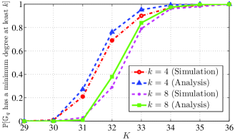
Figure 1: A plot of the probability that graph $\mathbb{G}_{q}(n,K,P,p)$ has a minimum node degree at least $k$ as a function of $K$ for $k=4$ and $k=8$ with $n=2,000$, $q=2$, $P=10,000$, and $p=0.8$.

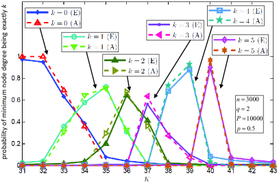
Figure 2: A plot of the probability that graph $\mathbb{G}_{q}(n,K,P,p)$’s minimum node degree equals $k$ exactly as a function of $K$ for $k=0,1,2,3,4,5$ with $n=3000$, $q=2$, $P=10000$, and $p=0.5$.

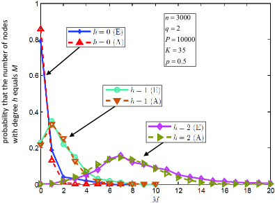
Figure 3: A plot of the probability distribution for the number of nodes with degree $h$ for $h=0,1,2$ in graph $\mathbb{G}_{q}(n,K,P,p)$ with $n=3000$, $q=2$, $P=10000$, $K=35$ and $p=0.5$.

In Figure 1, we depict the probability that graph $\mathbb{G}_{q}(n,K,P,p)$ has a minimum node degree at least $k$ from both the simulation and the analysis, for $k=4,8$ and $K$ varying from 29 to 36 (we set $n=2,000$, $q=2$ and $P=10,000$ and $p=0.8$). On the one hand, for the experimental curves in all figures, we generate $2,000$ independent samples of $\mathbb{G}_{q}(n,K,P,p)$ given a parameter set and record the count (out of a possible $2,000$) that the minimum degree of graph $\mathbb{G}_{q}(n,K,P,p)$ is no less than $k$. Then the empirical probabilities are obtained by dividing the counts by $2,000$. On the other hand, we approximate the analytical curves of Figure 1 by the asymptotic results as explained below. First, we compute the corresponding probability of $p_{e,q}$ in $\mathbb{G}_{q}(n,K,P,p)$ through $p_{e,q}=p\cdot\sum_{u=q}^{K}\big{[}{\binom{K}{u}\binom{P-K}{K-u}}\big{/}{\binom{P}{K}}\big{]}$ given (8) and $P>2K$. Then we determine $\alpha$ by (9) (we write $\alpha_{n}$ as $\alpha$ here as $n$ is fixed); i.e., $p_{e,q}=\frac{\ln n+{(k-1)}\ln\ln n+{\alpha}}{n}$. Then given Remark 1 after Theorem 1, we plot the analytical curves by considering that the minimum degree of $\mathbb{G}_{q}(n,K,P,p)$ is at least $k$ with probability $e^{-\frac{e^{-\alpha}}{(k-1)!}}$. The observation that the simulation and the analytical curves in Figure 1 are close is in accordance with Theorem 1.

In Figures 2 and 3, the curves with legends labelled “(E)” are experimental curves produced from experiments, while the curves with legends labelled “(A)” are analytical curves generated from theoretical analysis. In Figure 2, we depict the probability that graph $\mathbb{G}_{q}(n,K,P,p)$’s minimum node degree equals $k$ exactly as a function of $K$ for $k=0,1,2,3,4,5$. We set $n=3000$, $q=2$, and $P=10000$, and $p=0.5$. For the experimental curves, we generate $2000$ independent samples of graph $\mathbb{G}_{q}(n,K,P,p)$ and record the count that the minimum degree of graph $\mathbb{G}_{q}(n,K,P,p)$ is exactly $k$; and the empirical probability of $\mathbb{G}_{q}(n,K,P,p)$ having a minimum degree of $k$ is derived by averaging over the $2000$ experiments. The analytical curves are produced as follows. First, we compute the corresponding probability of $p_{e,q}$ in $\mathbb{G}_{q}(n,K,P,p)$ through the aforementioned expression $p_{e,q}=p\cdot\big{\{}1-\sum_{u=0}^{q-1}\big{[}{\binom{K}{u}\binom{P-K}{K-u}}\big{/}{\binom{P}{K}}\big{]}\big{\}}$. Then we select $\ell^{*}$ such that $\big{|}p_{e,q}-\frac{\ln n+(\ell-1)\ln\ln n}{n}\big{|}$ is minimized for integer $\ell$ (i.e., $\ell^{*}=\operatornamewithlimits{argmin}_{\textrm{integer }\ell}\big{|}p_{e,q}-\frac{\ln n+(\ell-1)\ln\ln n}{n}\big{|}$) and further define $\gamma^{*}$ such that $p_{e,q}=\frac{\ln n+(\ell-1)\ln\ln n+\gamma^{*}}{n}$. Given Remark 2 after Theorem 2, we plot the analytical curves by considering that i) if $\ell^{*}>0$, then ${\mathbb{P}}\left[{\delta=k}\right]$ equals $e^{-\frac{e^{-\gamma^{*}}}{(\ell^{*}-1)!}}$ for $k=\ell^{*}$, equals $1-e^{-\frac{e^{-\gamma^{*}}}{(\ell^{*}-1)!}}$ for $k=\ell^{*}-1$, and equals $0$ for $k\neq\ell^{*}$ and $k\neq\ell^{*}-1$, and ii) if $\ell^{*}\leq 0$, then ${\mathbb{P}}\left[{\delta=k}\right]$ equals $1$ for $k=0$, and equals $0$ for $k\neq 0$. The observation that the curves generated from the experimental and the analytical curves are close to each other confirms the result on the distribution of the minimum degree in Theorem 2.

In Figure 3, we plot the probability distribution for the number of nodes with degree $h$ in graph $\mathbb{G}_{q}(n,K,P,p)$ for $h=0,1,2$ from both the experiments and the analysis. We set $n=3000$, $q=2$, $K=35$, $P=10000$, and $p=0.5$. On the one hand, for the experiments, we generate $2000$ independent samples of $\mathbb{G}_{q}(n,K,P,p)$ and record the count (out of a possible $2000$) that the number of nodes with degree $h$ for each $h$ equals a particular non-negative number $M$. Then the empirical probabilities are obtained by dividing the counts by $2000$. On the other hand, we approximate the analytical curves by the asymptotic results as explained below. In Theorem 3, we establish that the number of nodes in $\mathbb{G}_{q}(n,K_{n},P_{n},p_{n})$ with degree $h$ approaches to a Poisson distribution with mean $\lambda_{n,h}=n(h!)^{-1}(np_{e,q})^{h}e^{-np_{e,q}}$ as $n\to\infty$. We derive $\lambda_{n,h}$ by computing the corresponding probability of $p_{e,q}$ in $\mathbb{G}_{q}(n,K,P,p)$ through $p_{e,q}=p\cdot\big{\{}1-\sum_{u=0}^{q-1}\big{[}{\binom{K}{u}\binom{P-K}{K-u}}\big{/}{\binom{P}{K}}\big{]}\big{\}}$ as explained above. Then for each $h$, we plot a Poisson distribution with mean $\lambda_{n,h}$ as the curve corresponding to the analysis. In Figure 3, we observe that the curves generated from the experiments and those obtained by the analysis are close to each other, confirming the result on asymptotic Poisson distribution in Theorem 3.

X Related Work

Erdős and Rényi [21] propose the random graph model $G(n,p_{n})$ defined on a node set with size $n$ such that an edge between any two nodes exists with probability $p_{n}$ independently of all other edges. For graph $G(n,p_{n})$, Erdős and Rényi [21] derive the asymptotically exact probabilities for connectivity and the property that the minimum degree is at least $1$, by proving first that the number of isolated nodes converges to a Poisson distribution as $n\to\infty$. Later, they extend the results to general $k$ in [26], obtaining the asymptotic Poisson distribution for the number of nodes with any degree and the asymptotically exact probabilities for $k$-connectivity and the event that the minimum degree is at least $k$, where $k$-connectivity is defined as the property that the network remains connected in spite of the removal of any $(k-1)$ nodes.

Recall that graph $\mathbb{G}_{q}(n,K_{n},P_{n})$ models the topology of the $q$-composite key predistribution scheme [27, 28, 29]. For graph $\mathbb{G}_{q}(n,K_{n},P_{n})$, Bloznelis et al. [4] demonstrate that a connected component with at at least a constant fraction of $n$ emerges asymptotically when probability $p_{e,q}$ exceeds $1/n$. Recently, still for $G_{q}(n,K_{n},P_{n})$, Bloznelis [14] establishes the asymptotic Poisson distribution for the number of nodes with any degree. Our results in Theorem 3 by setting $p_{n}$ as $1$ imply his result; in particular, the result that he obtains is a special case of property (a) in our Theorem 3.

Yağan [5] presents zero-one laws in graph $\mathbb{G}_{1}$ (our graph $\mathbb{G}_{q}$ in the case of $q=1$) for connectivity and for the property that the minimum degree is at least $1$. Zhao et al. extend Yağan’s results to general $k$ for $\mathbb{G}_{1}$ in [3, 20]. Our results in this paper apply to general $q$, yet the corresponding results for $q=1$ are already stronger than those in [5, 20, 3].

Krishnan et al. [16] and Krzywdziński and Rybarczyk [7] describe results for the probability of connectivity asymptotically converging to 1 in WSNs employing the $q$-composite key predistribution scheme with $q=1$ (i.e., the Eschenauer-Gligor key predistribution scheme), not under the on/off channel model but under the well-known disk model [16, 7, 30, 31], where nodes are distributed over a bounded region of a Euclidean plane, and two nodes have to be within a certain distance for communication. Simulation results in our work [3] indicate that for WSNs under the key predistribution scheme with $q=1$, when the on-off channel model is replaced by the disk model, the performances for $k$-connectivity and for the property that the minimum degree is at least $k$ do not change significantly.

XI Conclusion and Future Work

In this paper, we analyze topological properties in WSNs operating under the $q$-composite key predistribution scheme with on/off channels. Experiments are shown to be in agreement with our theoretical findings. A future research direction is to consider communication models different from the on/off channel model.

-A Additional Lemmas

Lemma 2.

The following two properties hold, where $p_{s,q}$ denotes the probability that two nodes in graph $\mathbb{G}_{q}$ share at least $q$ keys:

• If $K_{n}=\omega(1)$ and $\frac{{K_{n}}^{2}}{P_{n}}=o(1)$, then
  $p_{s,q}=\frac{1}{q!}\big{(}\frac{{K_{n}}^{2}}{P_{n}}\big{)}^{q}\times[1\pm o(1)]$; i.e., $p_{s,q}\sim\frac{1}{q!}\big{(}\frac{{K_{n}}^{2}}{P_{n}}\big{)}^{q}$.

• If $K_{n}=\omega(\ln n)$ and $\frac{{K_{n}}^{2}}{P_{n}}=o\big{(}\frac{1}{\ln n}\big{)}$, then
  $p_{s,q}=\frac{1}{q!}\big{(}\frac{{K_{n}}^{2}}{P_{n}}\big{)}^{q}\times[1\pm o\big{(}\frac{1}{\ln n}\big{)}]$.

Lemma 3.

In graph $\mathbb{G}_{q}$, with $p_{e,q}$ denoting the probability that two distinct nodes have a secure link in between, for any $\mathcal{T}_{m}^{*}=(S_{1}^{*},S_{2}^{*},\ldots,S_{m}^{*})\in\mathbb{T}_{m}$ and any node $w\in\overline{\mathcal{V}_{m}}$, we obtain

$$\mathbb{P}[w\in M_{0^{m}}\boldsymbol{\mid}\mathcal{T}_{m}=\mathcal{T}_{m}^{*}]\geq 1-mp_{e,q},$$ (109)

and for any $i=1,2,\ldots,m$,

$$\mathbb{P}\big{[}w\in M_{0^{i-1},1,0^{m-i}}\boldsymbol{\mid}\mathcal{T}_{m}=\mathcal{T}_{m}^{*}\big{]}\leq p_{e,q};$$ (110)

and if $\frac{{K_{n}}^{2}}{P_{n}}=o(1)$, the following (111) and (112) hold:

$$\mathbb{P}[w\in M_{0^{m}}\boldsymbol{\mid}\mathcal{T}_{m}=\mathcal{T}_{m}^{*}]$$

$$\quad\leq e^{-mp_{e,q}+(q+2)!\binom{m}{2}{(p_{e,q})}^{\frac{q+1}{q}}+\frac{p_{e,q}p_{n}}{K_{n}}\sum_{1\leq i<j\leq m}|S_{ij}^{*}|},$$ (111)

and for any $i=1,2,\ldots,m$,

$$\mathbb{P}\big{[}w\in M_{0^{i-1},1,0^{m-i}}\boldsymbol{\mid}\mathcal{T}_{m}=\mathcal{T}_{m}^{*}\big{]}$$

$$\quad\geq p_{e,q}\bigg{[}1-(q+2)!m{(p_{e,q})}^{\frac{1}{q}}-\frac{p_{n}}{K_{n}}\sum_{j\in\{1,2,\ldots,m\}\setminus\{i\}}|S_{ij}^{*}|\bigg{]},$$ (112)

where $S_{ij}^{*}=S_{i}^{*}\cap S_{j}^{*}$.

Lemma 4.

In graph $\mathbb{G}_{q}$, if $\frac{{K_{n}}^{2}}{P_{n}}=o(1)$, then for any three distinct nodes $v_{i},v_{j}$ and $v_{t}$ and for any $u=0,1,\ldots,K_{n}$, we obtain that with sufficiently large $n$,

$$\mathbb{P}[({\Gamma}_{it}\cap{\Gamma}_{jt}\boldsymbol{\mid}(|S_{ij}|=u)]\leq\frac{p_{s,q}u}{K_{n}}+(q+2)!\cdot({p_{s,q})}^{\frac{q+1}{q}}.$$

Due to space limitation, we provide the proofs of Lemmas 2, 3, 4 in Appendices B, C, D of the full version [22].

References

[1]
H. Chan, A. Perrig, and D. Song, “Random key predistribution schemes for
sensor networks,” in IEEE Symposium on Security and Privacy, May 2003.
[2]
L. Eschenauer and V. Gligor, “A key-management scheme for distributed sensor
networks,” in ACM Conference on Computer and Communications Security
(CCS), 2002.
[3]
J. Zhao, O. Yağan, and V. Gligor, “-Connectivity in random key graphs
with unreliable links,” IEEE Transactions on Information Theory,
vol. 61, pp. 3810–3836, July 2015.
[4]
M. Bloznelis, J. Jaworski, and K. Rybarczyk, “Component evolution in a secure
wireless sensor network,” Networks, vol. 53, pp. 19–26, January 2009.
[5]
O. Yağan, “Performance of the Eschenauer–Gligor key distribution scheme
under an on/off channel,” IEEE Transactions on Information Theory,
vol. 58, pp. 3821–3835, June 2012.
[6]
J. Zhao, “On resilience and connectivity of secure wireless sensor networks
under node capture attacks,” IEEE Transactions on Information Forensics
and Security, 2016.
[7]
K. Krzywdziński and K. Rybarczyk, “Geometric graphs with randomly deleted
edges – Connectivity and routing protocols,” Mathematical
Foundations of Computer Science, vol. 6907, pp. 544–555, 2011.
[8]
K. Rybarczyk, “Diameter, connectivity and phase transition of the uniform
random intersection graph,” Discrete Mathematics, vol. 311, 2011.
[9]
J. Zhao, “Threshold functions in random s-intersection graphs,” in 2015
53rd Annual Allerton Conference on Communication, Control, and Computing
(Allerton), pp. 1358–1365, 2015.
[10]
O. Yağan and A. M. Makowski, “Zero–one laws for connectivity in random
key graphs,” IEEE Transactions on Information Theory, vol. 58,
pp. 2983–2999, May 2012.
[11]
J. Zhao, “On the resilience to node capture attacks of secure wireless sensor
networks,” in Allerton Conference on Communication, Control, and
Computing (Allerton), pp. 887–893, 2015.
[12]
S. E. Nikoletseas and C. L. Raptopoulos, “On some combinatorial properties of
random intersection graphs,” in Algorithms, Probability, Networks, and
Games, pp. 370–383, 2015.
[13]
J. Zhao, “Modeling interest-based social networks: Superimposing
Erdos–Renyi graphs over random intersection graphs,” in IEEE
International Conference on Acoustics, Speech and Signal Processing
(ICASSP), 2017.
[14]
M. Bloznelis, “Degree and clustering coefficient in sparse random intersection
graphs,” The Annals of Applied Probability, vol. 23, no. 3,
pp. 1254–1289, 2013.
[15]
J. Zhao, “Parameter control in predistribution schemes of cryptographic
keys,” in IEEE Global Conference on Signal and Information Processing
(GlobalSIP), pp. 863–867, 2015.
[16]
B. Krishnan, A. Ganesh, and D. Manjunath, “On connectivity thresholds in
superposition of random key graphs on random geometric graphs,” in IEEE
International Symposium on Information Theory (ISIT), pp. 2389–2393, 2013.
[17]
J. Zhao, “Designing secure networks under -composite key predistribution
with unreliable links,” in IEEE International Conference on Acoustics,
Speech and Signal Processing (ICASSP), 2017.
[18]
E. M. Shahrivar, M. Pirani, and S. Sundaram, “Robustness and algebraic
connectivity of random interdependent networks,” IFAC-PapersOnLine,
vol. 48, no. 22, pp. 252–257, 2015.
[19]
S. M. Dibaji and H. Ishii, “Consensus of second-order multi-agent systems in
the presence of locally bounded faults,” Systems & Control Letters,
vol. 79, pp. 23–29, 2015.
[20]
J. Zhao, O. Yağan, and V. Gligor, “Secure -connectivity in wireless
sensor networks under an on/off channel model,” in IEEE International
Symposium on Information Theory (ISIT), pp. 2790–2794, 2013.
[21]
P. Erdős and A. Rényi, “On random graphs, I,” Publicationes
Mathematicae (Debrecen), vol. 6, pp. 290–297, 1959.
[22]
J. Zhao, “Topological properties of secure wireless sensor networks under the
-composite key predistribution scheme with unreliable links,” 2016.
Full version of this paper, available online at
https://sites.google.com/site/workofzhao/qcomposite.pdf
[23]
R. Di Pietro, L. V. Mancini, A. Mei, A. Panconesi, and J. Radhakrishnan,
“Redoubtable sensor networks,” ACM Transactions on Information and
System Security (TISSEC), vol. 11, pp. 13:1–13:22, March 2008.
[24]
J. Zhao, “Topology control in secure wireless sensor networks,” in Cyber
Security for Industrial Control Systems: From the Viewpoint of Close-Loop
(P. Cheng, H. Zhang, and J. Chen, eds.), ch. 8, pp. 183–224, CRC Press,
2016.
[25]
A. DasGupta, Asymptotic Theory of Statistics and Probability, vol. XVII.
Springer Texts in Statistics, 2008.
[26]
P. Erdős and A. Rényi, “On the strength of connectedness of random
graphs,” Acta Mathematica Academiae Scientiarum Hungarice,
pp. 261–267, 1961.
[27]
J. Zhao, O. Yağan, and V. Gligor, “On -connectivity and minimum vertex
degree in random -intersection graphs,” in ACM-SIAM Meeting on
Analytic Algorithmics and Combinatorics (ANALCO), pp. 1–15, January 2015.
[28]
M. Farrell, T. D. Goodrich, N. Lemons, F. Reidl, F. S. Villaamil, and B. D.
Sullivan, “Hyperbolicity, degeneracy, and expansion of random intersection
graphs,” in International Workshop on Algorithms and Models for the
Web-Graph, pp. 29–41, 2015.
[29]
J. Zhao, O. Yağan, and V. Gligor, “On topological properties of wireless
sensor networks under the q-composite key predistribution scheme with on/off
channels,” in IEEE International Symposium on Information Theory
(ISIT), pp. 1131–1135, June 2014.
[30]
J. Zhao, O. Yağan, and V. Gligor, “Connectivity in secure wireless sensor
networks under transmission constraints,” in Allerton Conference on
Communication, Control, and Computing, pp. 1294–1301, 2014.
[31]
J. Pandey and B. Gupta, “Distribution of -connectivity in the secure
wireless sensor network,” in International Conference on Recent
Advances and Innovations in Engineering (ICRAIE), pp. 1–6, May 2014.