Optimal Robust Learning of Discrete Distributions from Batches

Abstract

Many applications, including natural language processing, sensor networks, collaborative filtering, and federated learning, call for estimating discrete distributions from data collected in batches, some of which may be untrustworthy, erroneous, faulty, or even adversarial.

Previous estimators for this setting ran in exponential time, and for some regimes required a suboptimal number of batches. We provide the first polynomial-time estimator that is optimal in the number of batches and achieves essentially the best possible estimation accuracy.

1 Introduction

1.1 Motivation

Estimating discrete distributions from their samples is a fundamental modern-science tenet. [KOPS15] showed that as the number of sample $s$ grows, a $k$-symbol distribution can be learned to expected $L_{1}$ distance $\sim\sqrt{2(k\!-\!1)/(\pi s)}$ that we call the information-theoretic limit.

In many applications, some samples are inadvertently or maliciously corrupted. A simple and intuitive example shows that this erroneous data limits the extent to which a distribution can be learned, even with infinitely many samples.

Consider the extremely simple case of just two possible binary distributions: $(1,0)$ and $(1-\beta,\beta)$. An adversary who observes a $1-\beta$ fraction of the samples and can determine the rest, could use the observed samples to learn the underlying distribution, and set the remaining samples to make the distribution appear to be $(1-\beta,\beta)$. By the triangle inequality, even with arbitrarily many samples, any estimator for $p$ incurs an $L_{1}$ loss $\geq\beta$ for at least one of the two distributions. We call this the adversarial lower bound.

The example may seem to suggest a pessimistic conclusion. If an adversary can corrupt a $\beta$ fraction of the data, a loss $\geq\beta$ is unavoidable. Fortunately, that is not necessarily so.

In many applications data is collected in batches, most of which are genuine, but some possibly corrupted. Here are a few examples. Data may be gathered by sensors, each providing a large amount of data, and some sensors may be faulty. The word frequency of an author may be estimated from several large texts, some of which are mis-attributed. Or user preferences may be learned by querying several users, but some users may intentionally bias their feedback.

Interestingly, even when a $\beta$-fraction of the batches are corrupted, the underlying distribution can be estimated to $L_{1}$ distance much lower than $\beta$. Consider for example just three $n$-sample batches, of which one is chosen adversarially. The underlying distribution can be learned from each genuine batch to expected $L_{1}$ distance $\sim\sqrt{2(k-1)/(\pi n)}$. It is easy to see that the average of the two estimates pairwise-closest in $L_{1}$ distance achieves a comparable expected distance that large batch size $n$ is much lower than $\beta$.

This raises the natural question of whether estimates from even more batches can be combined effectively to estimate distributions to within a distance that is not only much smaller than the $\beta$ achieved when no batch information was utilized, but also significantly smaller than the $O(\sqrt{k/n})$ distance derived above when two batches were used. For example can the underlying distribution be learned to a small $L_{1}$ distance when, as in many practical examples, $n\leq k$?

To formalize the problem, [QV17] considered learning a $k$-symbol distribution $p$ whose samples are provided in batches of size $\geq n$. A total of $m$ batches are provided, of which a fraction $\leq\beta$ may be arbitrarily and adversarially corrupted, while in every other batch $b$ the samples are drawn according a distribution $p_{b}$ satisfying $||p_{b}-p||_{1}\leq\eta$, allowing for the possibility that slightly different distributions generate samples in each batch.

For this adversarial batch setting, they showed that for any alphabet size $k\geq 2$, and any number $m$ of batches, the lowest achievable $L_{1}$ distance is $\geq\eta+\frac{\beta}{\sqrt{2n}}$. We refer to this as the adversarial batch lower bound.

For $\beta\!<\!1/900$, they also derived an estimation algorithm that approximates $p$ to $L_{1}$ distance $O(\max\{\eta+\beta/\sqrt{n},\allowbreak\sqrt{(n+k)/(nm)}\})$, achieving the adversarial batch lower bound. Surprisingly therefore, not only can the underlying distribution be approximated to $L_{1}$ distance $O(\sqrt{k/n})$ that falls below $\beta$, but the distance diminishes as $\beta/\sqrt{n}$, independent of the alphabet size $k$, given sufficient number of batches $m$.

Yet, the algorithm in [QV17] had three significant drawbacks. 1) it runs in time exponential in the alphabet size, hence impractical for most relevant applications; 2) its guarantees are limited to very small fractions of corrupted batches $\beta\geq 1/900$, hence do not apply to practically important ranges; 3) with $m$ batches of size $\geq n$ each, the total number of samples is $\geq nm$, and for alphabet size $k\ll n$, the algorithm’s distance guarantee falls short of the information-theoretic $\Theta(\sqrt{k/(nm)})$ limit.

In this paper we derive an algorithm that 1) runs in polynomial time in all parameters; 2) can tolerate any fraction of adversarial batches $\beta<1/2$, though to derive concrete constant factors in the theoretical analysis, we assume $\beta\leq 0.4$; 3) achieves distortion $O(\max\{\eta+\beta\sqrt{\frac{\log(1/\beta)}{{n}}},\sqrt{\frac{k}{nm}}\})$ that achieves the statistical limit in terms of the number $nm$ of samples, and is optimal up to a small $O(\sqrt{\log(1/\beta)})$ factor from the adversarial batch lower bound.

The algorithm’s computational efficiency, enables the first experiments of learning with adversarial batches. We tested the algorithm on simulated data with various adversarial-batch distributions and adversarial noise levels up to $\beta=0.49$. The algorithm runs in a fraction of a second, and as shown in Section 3, estimates $p$ nearly as well as an oracle that knows the identity of the adversarial batches.

To summarize, the algorithm runs in polynomial time, works for any adversarial fraction $\beta<0.5$, is optimal in number of samples, and essentially optimal in batch size. It opens the door to practical robust estimation in sensor networks, federated learning, and collaborative filtering.

1.2 Problem Formulation

Let $\Delta_{k}$ be the collection of all distributions over $[k]={\{1{,}\ldots{,}k\}}$. The $L_{1}$ distance between two distributions $p,q\in\Delta_{k}$ is

$$||p-q||_{1}\triangleq\sum_{i\in[k]}|p(i)-q(i)|=2\cdot\max_{S\subseteq[k]}|p(S)-q(S)|.$$

We would like to estimate an unknown target distribution $p\in\Delta_{k}$ to a small $L_{1}$ distance from samples, some of which may be corrupted or even adversarial.

Specifically, let $B$ be a collections of $m$ batches of $n$ samples each. Among these batches is an unknown collection of good batches ${B}_{G}\subseteq B$; each batch $b\in{B}_{G}$ in this collection has $n$ independent samples $X^{b}_{1},X^{b}_{2},...,X^{b}_{n}\sim p_{b}$ with $||p_{b}-p||_{1}\leq\eta$. Furthermore, the batches of samples in ${B}_{G}$ are independent of each other.

For the special case where $\eta=0$, all samples in the good batches are generated by the target distribution $p=p_{b}$. Since the proofs and techniques are essentially the same for $\eta=0$ and $\eta>0$, for simplicity of presentation we assume that $\eta=0$. We briefly discuss, at the end, how these results translate to the case $\eta>0$.

The remaining set ${B}_{A}={B}\setminus{B}_{G}$ of adversarial batches consists of arbitrary $n$ samples each, that may even be chosen by an adversary, possibly based on the samples in the good batches. Let $\alpha=|{{B}_{G}}|/m$, and $\beta=|{{B}_{A}}|/m=1-\alpha$ be the fractions of good and adversarial batches, respectively.

Our goal is to use the $m$ batches to return a distribution $p^{*}$ such that $||p^{*}-p||_{1}$ is small or equivalently $|p(S)-p^{*}(S)|$ is small for all $S\subseteq[k]$.

1.3 Result Summary

In section 2 we derive a polynomial-time algorithm that returns an estimate $p^{*}$ of $p$ with the following properties.

Theorem 1.

For any given $\beta\leq 0.4$, $n$, $k$, and $m\geq O(\frac{k}{\beta^{2}\log(1/\beta)})$, Algorithm 2 runs in time polynomial in all parameters and its estimate $p^{*}$ satisfies $||p^{*}-p||_{1}\leq 100\beta\sqrt{\frac{\log(1/\beta)}{n}}$ with probability $\geq 1-O(e^{-k})$.

The theorem implies that our algorithm can achieve the adversarial lower bound to a small factor of $O(\sqrt{\log(1/\beta)})$ using the optimal number of samples. The next corollary shows that when the number of samples is not enough to achieve the adversarial batch lower bound our algorithm achieves the statistical lower bound.

If the number of batches $m\ll\frac{k}{\beta^{2}\log(1/\beta)}$, then let $\beta_{*}$ such that $m=\Theta{\left({\frac{k}{\beta_{*}^{2}\log(1/\beta_{*})}}\right)}$. Clearly, $\beta_{*}\gg\beta$. From Theorem 1, the algorithm would achieve a distance $O{\left({\beta_{*}\sqrt{\frac{\log(1/\beta_{*})}{n}}}\right)}=O{\left({\sqrt{\frac{k}{nm}}}\right)}$. We get the following corollary.

Corollary 2.

For any given $\beta\leq 0.4$, $n$ and $k$ and $m\gg k$, Algorithm 2 runs in polynomial time, and its estimate $p^{*}$ satisfies $||p^{*}-p||_{1}\leq O(\max\{\beta\sqrt{\frac{\ln(1/\beta)}{n}},\sqrt{\frac{k}{mn}}\})$ with probability $\geq 1-O(e^{-k})$.

Note that our polynomial time algorithm achieves the statistical limits for $L_{1}$ distance and achieves the adversarial batch lower bounds to a small multiplicative factor of $O(\sqrt{\log(1/\beta)})$.

1.4 Comparison to Recent Results and techniques

In a paper concurrent and independent of this work, [CLM19] propose an algorithm that uses the sum of squares methodology to estimates $p$ to the same distance as ours. Their algorithm need $\tilde{O}(\frac{(nk)^{O(\log(1/\beta))}}{\beta^{4}})$ batches and has a run-time $\tilde{O}(\frac{(nk)^{O(\log^{2}(1/\beta))}}{\beta^{O(\log(1/\beta))}})$. Both the sample complexity and run time are much higher than ours, and is quasi-polynomial. They also consider certain structured distributions, not addressed in this paper, for which they provide an algorithm with similar run time, but lower sample complexity.

1.5 Other Related Work

The current results extend several long lines of work on learning distributions and their properties.

The best approximation of a distribution with a given number of samples was determined up to the exact first-order constant for KL loss [BS04], and $L_{1}$ loss and $\chi^{2}$ loss [KOPS15]. These settings do not allow adversarial examples, and some modification of the empirical estimates of the samples is often shown to be near optimal. This is not the case in the presence of adversarial samples, where the challenge is to devise algorithms that are efficient from both computational and sample viewpoints.

Our results also relate to classical robust-statistics work [Tuk60, Hub92]. There has also been significant recent work leading to practical distribution learning algorithms that are robust to adversarial contamination of the data. For example, [DKK⁺16, LRV16] presented algorithms for learning the mean and covariance matrix of high-dimensional sub-gaussian and other distributions with bounded fourth moments in presence of the adversarial samples. Their estimation guarantees are typically in terms of $L_{2}$, and do not yield the $L_{1}$- distance results required for discrete distributions.

The work was extended in [CSV17] to the case when more than half of the samples are adversarial. Their algorithm returns a small set of candidate distributions one of which is a good approximate of the underlying distribution. For more extensive survey on robust learning algorithms in the continuous setting, see [SCV17, DKK⁺19].

Another motivation for this work derives from the practical federated-learning problem, where information arrives in batches [MMR⁺16, MR17].

1.6 Preliminaries

We introduce notation that will help outline our approach and will be used in rest of the paper.

Throughout the paper, we use ${B}^{\prime}$ to denote a sub-collection of batches in ${B}$ and use ${B}^{\prime}_{G}$ and ${B}^{\prime}_{A}$ for a sub-collection of batches in ${B}_{G}$ and ${B}_{A}$, respectively. And $S$ is used to denote a subset of $[k]$, we abbreviate singleton set of $[k]$ such as $\{j\}$ by $j$.

For any batch $b\in B$, we let ${\bar{\mu}_{b}}$ denote the empirical measure defined by samples in batch $b$. And for any sub-collection of batches ${B}^{\prime}\subseteq{B}$, let ${\bar{p}_{{B}^{\prime}}}$ denote the empirical measure defined by combined samples in all the batches in ${B}^{\prime}$. We use two different symbols to distinguish the empirical distribution defined by an individual batch and the empirical distribution defined by a sub-collection of batches. Let $\mathbf{1}_{S}(.)$ denote the indicator random variable for set $S$. Thus, for any subset $S\subseteq[k]$,

$${\bar{\mu}_{b}(S)}\triangleq\frac{1}{n}\sum_{i\in[n]}\mathbf{1}_{S}(X_{i}^{b})$$

and

$${\bar{p}_{{B}^{\prime}}(S)}\triangleq\frac{1}{|{B}^{\prime}|n}\sum_{b\in{B}^{\prime}}\sum_{i\in[n]}\mathbf{1}_{S}(X_{i}^{b})=\frac{1}{|{B}^{\prime}|}\sum_{b\in{B}^{\prime}}{\bar{\mu}_{b}(S)}.$$

Note that ${\bar{p}_{{B}^{\prime}}}$ is the mean of the empirical measures ${\bar{\mu}_{b}}$ defined by the batches $b\in{B}^{\prime}$. For subset $S\subseteq[k]$, let $\text{med}(\bar{\mu}(S))$ be the median of the set of estimates $\{{\bar{\mu}_{b}(S)}:b\in{B}\}$. Note that the median has been computed using the estimates ${\bar{\mu}_{b}(S)}$ for all the batches in $b\in{B}$.

For $r\in[0,1]$, we let $\text{V}(r)\triangleq\frac{r(1-r)}{n}$, which we use to denote the variance of sum of $n$ i.i.d. random variables distributed according to $\text{Bernoulli}(r)$.

We pause briefly to note the following two properties of the function $\text{V}(r)$ that we use later.

$$\forall\,r,s\in[0,1],\,\text{V}(r)\leq\frac{1}{4n}\text{ and }|\text{V}(r)-\text{V}(s)|\leq\frac{|r-s|}{n}.$$ (1)

Here the second property made use of the fact that the derivative $|V^{\prime}(r)|\leq 1/n,\,\forall\,r\in[0,1]$.

For $b\in{B}_{G}$, $\mathbf{1}_{S}(X_{i}^{b})$ for $i\in[n]$ are i.i.d. with distribution $\mathbf{1}_{S}(X_{i}^{b})\sim\text{Bernoulli}(p(S))$. For $b\in{B}_{G}$, since ${\bar{\mu}_{b}(S)}$ is average of $\mathbf{1}_{S}(X_{i}^{b})$, $i\in[n]$, therefore,

$$E[\,{\bar{\mu}_{b}(S)}\,]=p(S)\quad\text{ and }\quad E[({\bar{\mu}_{b}(S)}-p(S))^{2}]=\text{V}(p(S)).$$

For any collection of batches ${B}^{\prime}\subseteq{B}$ and subset $S\subseteq[k]$, the empirical probability ${\bar{\mu}_{b}(S)}$ of $S$ based on batches $b\in{B}^{\prime}$ will differ for the different batches. The empirical variance of these empirical probabilities ${\bar{\mu}_{b}(S)}$ for batches $b\in{B}^{\prime}$ is denoted as

$$\overline{\text{V}}_{{B}^{\prime}}(S)\triangleq\frac{1}{|{{B}^{\prime}}|}\sum_{b\in{{B}^{\prime}}}({\bar{\mu}_{b}(S)}-{\bar{p}_{{B}^{\prime}}(S)})^{2}.$$

1.7 Organization of the Paper

In Section 2 we present the algorithm, its analysis along with the key insights used in developing the algorithm. Section 3 reports the performance of the algorithm on experiments performed on the simulated data.

2 Algorithm and its Analysis

At a high level, our algorithm removes the adversarial batches — which are "outliers" — possibly losing a small number of good batches as well in the process. The outlier removal method forms the backbone of many robust learning algorithms. Notably [DKK⁺16, DKK⁺17] have used this idea to learn the mean of a high dimensional sub-gaussian distribution up to a small $L_{2}$ distance, even in an adversarial setting. The main challenge in designing a robust learning algorithm is actually the task of finding the outlier batches efficiently. Several new ideas are needed to identify the outlier batches in the setting considered here.

We begin by illustrating the difficulty of identifying the adversarial batches. Even if $p$ is known, in general, one cannot determine whether a batch $b$ has samples from $p$ or from a distribution at a large $L_{1}$ distance from $p$. The key difficulty is that, for a batch having $n$ samples from $p$, typically the difference between ${\bar{\mu}_{b}(S)}$ and $p(S)$ is large for some of the subsets among $2^{k}$ subsets of $[k]$. For example, consider batches of samples from a uniform distribution over $k$. The empirical distribution of the samples in any batch of size $n$ is at an $L_{1}$ distance $\geq 2(1-n/k)$, which for the distributions with large domain size $k$ can be up to two, which is the maximum $L_{1}$ distance between two distributions. To address this challenge, we use the following observation.

For a fixed subset $S\subseteq[k]$ and a good batch $b\in{B}_{G}$, ${\bar{\mu}_{b}(S)}$ has a sub-gaussian distribution $\text{subG}(p(S),\frac{1}{4{n}})$ and the variance is $\text{V}(p(S))$. Therefore, for a fixed subset $S$, most of the good batches assign the empirical probability ${\bar{\mu}_{b}(S)}\in p(S)\pm\tilde{O}(1/\sqrt{n})$. Moreover, the mean and the variance of ${\bar{\mu}_{b}(S)}$ for $b\in{B}_{G}$ converges to the expected values $p(S)$ and $\text{V}(p(S))$, respectively.

The collection of batches ${B}$ along with good batches also includes a sub-collection ${B}_{A}$ of adversarial batches that constitute up to an $\beta-$fraction of ${B}$. If for adversarial batches $b\in{B}_{A}$, the average difference between ${\bar{\mu}_{b}(S)}$ and $p(S)$ is within a few standard deviations $\tilde{O}(\frac{1}{\sqrt{n}})$, then these adversarial batches can only deviate the overall mean of empirical probabilities ${\bar{\mu}_{b}(S)}$ by $\tilde{O}(\frac{\beta}{\sqrt{n}})$ from $p(S)$. Hence, the mean of ${\bar{\mu}_{b}(S)}$ will deviates significantly from $p(S)$ only if for a large number of adversarial batches $b\in{B}_{A}$ empirical probability ${\bar{\mu}_{b}(S)}$ differ from $p(S)$ by quantity much larger than the standard deviation $\tilde{O}(\frac{1}{\sqrt{n}})$.

We quantify this effect by defining the corruption score. For a subset $S\subseteq[k]$, let

$$\text{med}(\bar{\mu}(S))\triangleq\text{median}\{{\bar{\mu}_{b}(S)}:b\in{B}\}.$$

For a subset $S\subseteq[k]$ and a batch $b$, corruption score $\psi_{b}(S)$ is defined as

$$\psi_{b}(S)\triangleq\begin{cases}0,\ \ \ \text{ if }\ |{\bar{\mu}_{b}(S)}-\text{med}(\bar{\mu}(S))|\leq 3\sqrt{\frac{\ln(6e/\beta)}{n}},\\ ({\bar{\mu}_{b}(S)}-\text{med}(\bar{\mu}(S)))^{2},\ \ \ \text{ else}.\end{cases}$$

Because $p(S)$ is not known, the above definition use median of ${\bar{\mu}_{b}(S)}$ as its proxy.

From the preceding discussion, it follows that for a fixed subset $S\subseteq[k]$, corruption score of most good batches w.r.t. $S$ is zero, and adversarial batches that may have a significant effect on the overall mean of empirical probabilities have high corruption score $\psi_{b}(S)$.

The corruption score of a sub-collection ${B}^{\prime}$ w.r.t. a subset $S$ is defined as the sum of the corruption score of batches in it, namely

$$\psi({B}^{\prime},S)\triangleq\sum_{b\in{B}^{\prime}}\psi_{b}(S).$$

A high corruption score of ${B}^{\prime}$ w.r.t. a subset $S$ indicates the presence of many batches $b\in{B}^{\prime}$ for which the difference $|{\bar{\mu}_{b}(S)}-\text{med}(\bar{\mu}(S))|$ is large. Finally, for a sub-collection ${B}^{\prime}$ we define corruption as

$$\psi({B}^{\prime})\triangleq\max_{S\subseteq[k]}\psi({B}^{\prime},S).$$

Note that removing batches from a sub-collection reduces corruption. We can simply make corruption zero by removing all batches, but we would lose all the information as well. The proposed algorithm reduces the corruption below a threshold by removing a few batches while not sacrificing too many good batches in the process.

The remainder of this section assumes that the sub-collection of good batches ${B}_{G}$ satisfies certain deterministic conditions. Lemma 3 shows that the stated conditions hold with high probability for sub-collection of good batches in ${B}_{G}$. Nothing is assumed about the adversarial batches, except that they form a $\leq\beta$ fraction of the overall batches ${B}$.

Conditions: Consider a collection of $m$ batches ${B}$, each containing $n$ samples. Among these batches, there is a collection ${B}_{G}\subseteq{B}$ of good batches of size $|{{B}_{G}}|\geq(1-\beta)m$ and a distribution $p\in\Delta_{k}$ such that the following deterministic conditions hold for all subsets $S\subseteq[k]$:

1. The median of the estimates $\{{\bar{\mu}_{b}(S)}:b\in{B}\}$ is not too far from $p(S)$.

   $$|\text{med}(\bar{\mu}(S))-p(S)|\leq\sqrt{\ln(6)/n}.$$

2. For all sub-collections ${B}^{\prime}_{G}\subseteq{B}_{G}$ of good batches of size $|{B}^{\prime}_{G}|\geq(1-\beta/6)|{{B}_{G}}|$,

   $$|{\bar{p}_{{B}^{\prime}_{G}}(S)}-p(S)|\leq\frac{\beta}{2}\sqrt{\frac{\ln(6e/\beta)}{n}},$$

   $$\Big{|}\frac{1}{|{B}^{\prime}_{G}|}\sum_{b\in{B}^{\prime}_{G}}({\bar{\mu}_{b}(S)}-p(S))^{2}-\text{V}(p(S))\Big{|}\leq{\frac{6\beta\ln(\frac{6e}{\beta})}{n}}.$$

3. The corruption for good batches ${B}_{G}$ is small, namely

   $$\psi({B}_{G})\leq{\frac{\beta m\ln({6e}/\beta)}{n}}.$$

Condition 1 and 3 above are self-explanatory. Condition 2 illustrates that for any sub-collection of good batches that retains all but a small fraction of good batches, empirical mean and variance estimate the actual values $p(S)$ and $\text{V}(p(S))$.

Lemma 3.

When samples in ${B}_{G}$ come from $p$ and $|{{B}_{G}}|\geq O(\frac{k}{\beta^{2}\ln(1/\beta)})$, then conditions 1- 3 hold simultaneously with probability $\geq 1-O(e^{-k})$.

We prove the above lemma by using the observation that for $b\in{B}_{G}$, ${\bar{\mu}_{b}(S)}$ has a sub-gaussian distribution $\text{subG}(p(S),\frac{1}{4n})$, and it has variance $\text{V}(p(S))$. The proof is in Appendix A.

For easy reference, in the remaining paper, we will denote the upper bound in Condition 3 on the corruption of ${B}_{G}$ as

$$\kappa_{G}\triangleq{\frac{\beta m\ln({6e}/\beta)}{n}}.$$

Assuming that the above stated conditions hold, the next lemma bounds the $L_{1}$ distance between the empirical distribution ${\bar{p}_{{B}^{\prime}}}$ and $p$ for any sub-collection ${B}^{\prime}$ in terms of how large its corruption is compared to $\kappa_{G}$.

Lemma 4.

Suppose the conditions 1- 3 holds. Then for any ${B}^{\prime}$ such that $|{B}^{\prime}\cap{B}_{G}|\geq(1-\frac{\beta}{6})|{{B}_{G}}|$ and let $\psi({B}^{\prime})=t\cdot\kappa_{G}$, for some $t\geq 0$, then

$$||{\bar{p}_{{B}^{\prime}}}-p||_{1}\leq(10+3\sqrt{t})\beta\sqrt{{\frac{\ln(6e/\beta)}{n}}}.$$

Observe that for any sub-collection ${B}^{\prime}$ retaining a major portion of good batches, from condition 2, the mean of ${\bar{\mu}_{b}}$ of the good batches ${B}^{\prime}\cap{B}_{G}$ approximates $p$. Then showing that a small corruption score of ${B}^{\prime}$ w.r.t. all subsets $S$ imply that the adversarial batches ${B}^{\prime}\cap{B}_{A}$ have limited effect on ${\bar{p}_{{B}^{\prime}}}$ proves the above lemma. A complete proof is in Appendix B.

We next exhibit a Batch Deletion procedure in 1 that lowers the corruption score of a sub-collection ${B}^{\prime}$ w.r.t. a given subset $S$ by deleting a few batches from the sub-Collection. This will be a subroutine of our main algorithm. Lemma 5 characterizes its performance.

Algorithm 1 Batch Deletion

1:  Input: Sub-Collection of Batches ${B}^{\prime}$, subset $S\subseteq[k]$, med=$\text{med}(\bar{\mu}(S))$, and $\beta$.

2:  Output: A collection $DEL\subseteq{B}^{\prime}$ of batches to delete.

3:  ${DEL}=\{\}$;

4:  while  $\psi({B}^{\prime},S)\,\geq\,20\kappa_{G}$ do

5:     Samples batch $b\in{B}^{\prime}$ such that probability of picking a batch $b\in{B}^{\prime}$ is $\frac{\psi_{b}(S)}{\psi({B}^{\prime},S)}$;

6:     $DEL\leftarrow DEL\cup{b}$ ;

7:     ${B}^{\prime}\leftarrow\{{B}^{\prime}\setminus{b}\}$;

8:  end while

9:  return $(DEL)$;

Lemma 5.

For a given ${B}^{\prime}$ and subset $S$ procedure 1 returns a sub-collection $DEL\subset{B}^{\prime}$, such that

1. For subset $S$ the corruption score $\psi({B}^{\prime}\setminus DEL,S)$ of the new sub-collection is $<20\kappa_{G}$.

2. Each batch $b\in{B}^{\prime}$ that gets included in $DEL$ is an adversarial batch with probability $\geq 0.95$.

3. The subroutine deletes at-least $\psi({B}^{\prime},S)-20\kappa_{G}$ batches.

Proof.

Step 4 in the algorithm ensures the first property. Next, to prove property 2, we bound the probability of deleting a good batch as

$$\sum_{b\in{B}^{\prime}\cap{B}_{G}}\frac{\psi_{b}(S)}{\psi({B}^{\prime},S)}\leq\frac{\sum_{b\in{B}_{G}}\psi_{b}(S)}{\psi({B}^{\prime},S)}\leq\frac{\kappa_{G}}{20\kappa_{G}},$$

here the last step follows from condition 3 and while loop conditional in step 4. Property 3 follows from the observation that the total corruption score reduced is $\geq(\psi({B}^{\prime},S)-20\kappa_{G})$ and corruption score of one batch is bounded as $\psi_{b}(S)\leq 1$. ∎

We will use procedure 1 to successively update ${B}$ to decrease the corruption score for different subsets $S\subseteq[k]$. The next lemma show that even after successive updates the resultant sub-collection retains most of the good batches.

Lemma 6.

Let ${B}^{\prime}$ be the sub-collection after applying any number of successive deletion updates suggested by the Algorithm 1 on ${B}$, for any sequence of input subsets $S_{1},S_{2},....\subseteq[k]$, then $|{B}^{\prime}\cap{B}_{G}|\geq(1-\beta/6)|{{B}_{G}}|$, with probability $\geq 1-O(e^{-k})$.

Therefore, one can make successive updates to the collection of all batches ${B}$ by deleting the batches suggested by procedure 1 for all subsets in $S\subseteq[k]$ one by one. This will result in a sub-collection ${B}^{\prime}\subseteq{B}$, which still has most of the good batches and corruption score $\psi({B}^{\prime},S)$ bounded w.r.t. each subset $S$. However, this will take time exponential in $k$ as there are $2^{k}$ subsets, and therefore, we want a computationally efficient method to find a subsets $S$ with high corruption score and use procedure 1 for only those subsets. Next, we derive a novel method to achieve this objective.

We start with the following observation. A high corruption score of sub-collection ${B}^{\prime}$ with respect to an affected subset $S$ implies a higher empirical variance of ${\bar{\mu}_{b}(S)}$ for such $S$ than the expected value of the variance of ${\bar{\mu}_{b}(S)}$. While an affected subset $S$ the empirical variance $\overline{\text{V}}_{{B}}(S)$ is higher than expected, it is not necessarily higher than the empirical variance observed for all non-affected subset. This is because $\text{V}(p(S))$, the expected value of the variance of ${\bar{\mu}_{b}(S)}$, for some subsets $S$ may be larger compared to the other. Hence, simply finding the subset $S$ with the largest variance doesn’t work.

We use the following key insight to address this. Recall that the mean of empirical probabilities ${\bar{\mu}_{b}(S)}$ for good batches $b\in{B}_{G}$ converges, or equivalently $\bar{p}_{{B}_{G}}(S)\rightarrow p(S)$. This implies that $\text{V}(\bar{p}_{{B}_{G}}(S))\rightarrow\text{V}(p(S))$. Also, since the empirical variance $\overline{\text{V}}_{{B}_{G}}(S)$ converges to $\text{V}(p(S))$, we get $\overline{\text{V}}_{{B}_{G}}(S)-\text{V}(\bar{p}_{{B}_{G}}(S))\rightarrow 0$. Therefore, without corruption by the adversarial batches the difference between two estimators of the variance would be small for all subsets $S\subseteq[k]$, and its large value, we show in Lemma 7, can reliably detect any significant adversarial corruption. This happens because empirical variance of ${\bar{\mu}_{b}(S)}$ depends on the second moment whereas the other estimator $\text{V}({\bar{p}_{{B}^{\prime}}(S)})$ of variance depends on the mean of ${\bar{\mu}_{b}(S)}$, hence the corruption affects the second estimator less severely. The next Lemma shows that the difference between the two variance estimators for subset $S$ can indicate the corruption score w.r.t. subset $S$

Lemma 7.

Suppose the conditions 1- 3 holds. Then for any ${B}^{\prime}\subseteq{B}$ such that $|{B}^{\prime}\cap{B}_{G}|\geq(1-\frac{\beta}{6})|{{B}_{G}}|$ and let $\psi({B}^{\prime},S)=t\cdot\kappa_{G}$ for some $t\geq 0$, then following holds.

$$\overline{\text{V}}_{{B}^{\prime}}(S)-\text{V}({\bar{p}_{{B}^{\prime}}(S)})\leq\Big{(}t+4\sqrt{t}+28\Big{)}\kappa_{G},$$

$$\overline{\text{V}}_{{B}^{\prime}}(S)-\text{V}({\bar{p}_{{B}^{\prime}}(S)})\geq\Big{(}0.5t-8\sqrt{t}-25\Big{)}\kappa_{G}.$$

The next Lemma shows that a subset for which $\overline{\text{V}}_{{B}^{\prime}}(S)-\text{V}({\bar{p}_{{B}^{\prime}}(S)})$ is large, can be found using a polynomial-time algorithm. In subsection 2.2 we derive the algorithm. We refer to this algorithm as $Detection-Algorithm$. The next lemma characterizes the performance of this algorithm. In subsection 2.2, we show that the algorithm achieves the performance guarantees of the next Lemma.

Lemma 8.

$Detection-Algorithm$ has run time polynomial in number of batches in its input sub-collection ${B}^{\prime}$ and alphabet size $k$, and returns $S^{*}_{{{B}^{\prime}}}$ such that

$$|\overline{{\text{V}}}_{{{B}^{\prime}}}(S^{*}_{{{B}^{\prime}}})-\text{V}({\bar{p}_{{B}^{\prime}}}(S^{*}_{{{B}^{\prime}}}))|$$

$$\geq 0.56\max_{S\subseteq[k]} |\overline{\text{V}}_{{B}^{\prime}}(S)-\text{V}({\bar{p}_{{B}^{\prime}}(S)})|.$$

This leads us to the Robust distribution Learning Algorithm 2. Theorem 9 characterizes its performance.

Algorithm 2 Robust Distribution Estimator

1:  Input: All batches $b\in{B}$, batch size $n$, alphabet size $k$, and $\beta$.

2:  Output: Estimate $p^{*}$ of the distribution $p$.

3:  $i\leftarrow 1$ and ${{B}^{\prime}_{i}}\leftarrow{B}$.

4:  while  True  do

5:     $S^{*}_{{{B}^{\prime}_{i}}}=Detection-Algorithm({B}^{\prime}_{i})$

6:     if $|\Delta_{{B}^{\prime}_{i}}(S^{*}_{{{B}^{\prime}_{i}}})|\leq 75\kappa_{G}$  then

7:        Break;

8:     end if

9:     $\text{med}\leftarrow\text{med}(\bar{\mu}(S^{*}_{{{B}^{\prime}_{i}}}))$.

10:     $DEL\leftarrow$Batch-Deletion(${B}^{\prime}_{i},S^{*}_{{{B}^{\prime}_{i}}},\text{med}$).

11:  end while

12:  return $(p^{*}\leftarrow\bar{p}_{{B}^{\prime}_{i}})$.

Theorem 9.

Suppose the conditions 1- 3 holds. Then Algorithm 2 runs in polynomial time and return a sub-collection ${B}^{\prime}_{f}\subseteq{B}$ such that $|{B}^{\prime}_{f}\cap{B}_{G}|\geq(1-\frac{\beta}{6})|{{B}_{G}}|$ and for $p^{*}={\bar{p}_{{B}^{\prime}_{f}}}$,

$$||p^{*}-p||_{1}\leq 100\beta\sqrt{\frac{\ln(6e/\beta)}{n}}.$$

Outline of the Proof of Theorem 9: In each round of the algorithm, Subroutine $Detection-Algorithm$ finds subsets for which the difference between the two variance estimates is large. Lemma 7 implies that the corruption w.r.t. this subset is large. The deletion subroutine updates the sub-collection of batches by removing some batches from it and reduces the corruption w.r.t. the detected subset $S$.

The algorithm terminates when for some sub-collection ${B}^{\prime}_{f}$ subroutine $Detection-Algorithm$ returns a subset $S$ small difference between the two variance estimators. Then Lemma 8 implies that the difference is small for all subsets. Lemma 7 further implies that if the difference between the two variance estimators is small then the corruption is bounded w.r.t. all subsets for sub-collection ${B}^{\prime}_{f}$. Finally, Lemma 4 bounds the $L_{1}$ distance between $\bar{p}_{{B}^{\prime}_{f}}$ and $p$.$\hfill\square$

Combining Lemma 3 and Theorem 9 yields Theorem 1.

2.1 Extension to $\eta>0$

Recall that when $\eta>0$, for each good batch $b\in{B}_{G}$, the distribution $p_{b}$ of samples in batch $b$ is close to the common target distribution $p$, such that $||p_{b}-p||\leq\eta$, instead of necessarily being the same. For simplicity, we have given the algorithm and the proof for only $\eta=0$. The algorithm and the proof naturally extend to this more general case; here we get an extra additive dependence on $\eta$ for the bounds in the lemmas and the theorems, and for the parameters of the algorithm. And with this slight modification in the parameters algorithm estimates $p$ to a distance $O(\eta+\beta\sqrt{\ln(1/\beta)/{n}})$, and has the same sample and time complexity.

2.2 Efficient Detection Algorithm

In this subsection, we derive the procedure $Detection-Algorithm$, that runs in the polynomial time and achieves the performance in Lemma 8.

Given a collection ${{B}^{\prime}}$ of batches, we construct two covariance matrices $C^{EV}_{{B}^{\prime}}$ and $C^{EM}_{{B}^{\prime}}$ of size $k\times k$.

For an alphabet size $k$, we can treat the empirical probabilities estimates ${\bar{\mu}_{b}}$ and ${\bar{p}_{{B}^{\prime}}}$ as a $k$-dimensional vector such that $j^{th}$ entry denote the empirical probability of the $j^{th}$ symbol. Recall that ${\bar{p}_{{B}^{\prime}}}$ is the mean of ${\bar{\mu}_{b}}$, $b\in{B}^{\prime}$.

The first covariance matrix, $C^{EV}_{{B}^{\prime}}$, is the covariance matrix of ${\bar{\mu}_{b}}$ for $b\in{B}^{\prime}$, with entries for $j,l\in[k]$,

$$C^{EV}_{{B}^{\prime}}(j,l)=\frac{1}{|{{B}^{\prime}}|}\sum_{b\in{{B}^{\prime}}}({\bar{\mu}_{b}}(j)-{\bar{p}_{{B}^{\prime}}}(j))({\bar{\mu}_{b}}(l)-{\bar{p}_{{B}^{\prime}}}(l)).$$

The second covariance matrix $C^{EM}_{{B}^{\prime}}$, is an expected covariance matrix of ${\bar{\mu}_{b}}$ if samples in the batches $b$ were drawn from the distribution ${\bar{p}_{{B}^{\prime}}}$. Hence, its entries are

$$C^{EM}_{{B}^{\prime}}(j,l)=-\frac{{\bar{p}_{{B}^{\prime}}}(j){\bar{p}_{{B}^{\prime}}}(l)}{n}\text{ for }j,l\in[k],\,j\neq l,$$

and

$$C^{EM}_{{B}^{\prime}}(j,j)=\frac{{\bar{p}_{{B}^{\prime}}}(j)(1-{\bar{p}_{{B}^{\prime}}}(j))}{n}.$$

Let $D_{{B}^{\prime}}$ be the difference of the two matrices:

$$D_{{B}^{\prime}}=C^{EV}_{{B}^{\prime}}-C^{EM}_{{B}^{\prime}}.$$

For a vector $x\in\{0,1\}^{k}$, let

$$S(x)\triangleq\{j\in[k]:x(j)=1\},$$

be the subset of $[k]$ corresponding to the vector $x$.

Observations

1. The sum of elements in any row and or column for both the covariance matrices, and hence also for the difference matrix, is zero, hence

   $$C^{EV}_{{B}^{\prime}}\boldsymbol{1}=C^{EM}_{{B}^{\prime}}\boldsymbol{1}=D_{{B}^{\prime}}\boldsymbol{1}=\boldsymbol{0}.$$

   Proof: We show for $C^{EV}_{{B}^{\prime}}$, the proof for $C^{EM}_{{B}^{\prime}}$ is similar. For any $j\in[k]$,

   $$\sum_{l\in[k]}C^{EV}_{{B}^{\prime}}(j,l)$$

   $$=\frac{1}{|{{B}^{\prime}}|}\sum_{l\in[k]}\sum_{b\in{{B}^{\prime}}}({\bar{\mu}_{b}}(j)-{\bar{p}_{{B}^{\prime}}}(j))({\bar{\mu}_{b}}(l)-{\bar{p}_{{B}^{\prime}}}(l))$$

   $$=\sum_{b\in{{B}^{\prime}}}({\bar{\mu}_{b}}(j)-{\bar{p}_{{B}^{\prime}}}(j))\sum_{l\in[k]}({\bar{\mu}_{b}}(l)-{\bar{p}_{{B}^{\prime}}}(l))$$

   $$=\sum_{b\in{{B}^{\prime}}}({\bar{\mu}_{b}}(j)-{\bar{p}_{{B}^{\prime}}}(j))(1-1)=0.$$

2. It is easy to verify that for any vector $x\in\{0,1\}^{k}$,

   $$\langle C^{EV}_{{B}^{\prime}},xx^{\intercal}\rangle =\frac{1}{|{{B}^{\prime}}|}\sum_{b\in{{B}^{\prime}}}({\bar{\mu}_{b}}(S(x))-{\bar{p}_{{B}^{\prime}}}(S(x)))^{2}$$

   $$=\overline{\text{V}}_{{{B}^{\prime}}}(S(x)),$$

   the empirical variance of ${\bar{\mu}_{b}}(S(x))$ for $b\in{{B}^{\prime}}$. Similarly,

   $$\langle C^{EM}_{{B}^{\prime}},xx^{\intercal}\rangle =\frac{{\bar{p}_{{B}^{\prime}}}(S(x))(1-{\bar{p}_{{B}^{\prime}}}(S(x)))}{n}$$

   $$=\text{V}({\bar{p}_{{B}^{\prime}}}(S(x))).$$

   Therefore,

   $$\langle D_{{B}^{\prime}},xx^{\intercal}\rangle =\langle C^{EV}_{{B}^{\prime}}-C^{EM}_{{B}^{\prime}},xx^{\intercal}\rangle$$

   $$=\overline{\text{V}}_{{{B}^{\prime}}}(S(x))-\text{V}({\bar{p}_{{B}^{\prime}}}(S(x))).$$

3. Note that $y\rightarrow\frac{1}{2}(y+\boldsymbol{1})$ is a 1-1 mapping from $\{-1,1\}^{k}\rightarrow\{0,1\}^{k}$, and that

   $$\langle C^{EV}_{{B}^{\prime}},\frac{1}{2}(y+\boldsymbol{1})\frac{1}{2}(y+\boldsymbol{1})^{\intercal}\rangle$$

   $$=\langle C^{EV}_{{B}^{\prime}},\frac{1}{4}(yy^{\intercal}+\boldsymbol{1}y^{\intercal}+y\boldsymbol{1}^{\intercal}+\boldsymbol{1}\boldsymbol{1}^{\intercal})\rangle$$

   $$=\frac{1}{4}\langle C^{EV}_{{B}^{\prime}},yy^{\intercal}\rangle.$$

Let

$$y=\arg\max_{y\in\{-1,1\}^{k}}|\langle D_{{B}^{\prime}},yy^{\intercal}\rangle|.$$

Then from $y$ one can recover the corresponding subset $S(x)$, with $x=\frac{1}{2}(y+\boldsymbol{1})$, maximizing

$$|\overline{\text{V}}_{{{B}^{\prime}}}(S(x))-\text{V}({\bar{p}_{{B}^{\prime}}}(S(x)))|.$$

In [AN04], Alon et al. derives a polynomial-time approximation algorithm for the above optimization problem. The algorithm first uses a semi-definite relaxation of the problem and then uses randomized integer rounding techniques based on Grothendieck’s Inequality. Their algorithm recovers $y_{{B}^{\prime}}$ such that

$$|\langle D_{{B}^{\prime}},y_{{B}^{\prime}}y_{{B}^{\prime}}^{\intercal}\rangle|\geq 0.56\max_{y\in\{-1,1\}^{k}}|\langle D_{{B}^{\prime}},yy^{\intercal}\rangle|.$$

Let $x_{{B}^{\prime}}=\frac{1}{2}(y+\boldsymbol{1})$. Then from observation 3 it follows that

$$|\langle D_{{B}^{\prime}},x_{{B}^{\prime}}x_{{B}^{\prime}}^{\intercal}\rangle|\geq 0.56\max_{x\in\{0,1\}^{k}}|\langle D_{{B}^{\prime}},xx^{\intercal}\rangle|.$$

Therefore for $S^{*}_{{B}^{\prime}}=S(x_{{B}^{\prime}})$ we get

$$|\overline{\text{V}}_{{{B}^{\prime}}}(S^{*}_{{B}^{\prime}})-\text{V}({\bar{p}_{{B}^{\prime}}}(S^{*}_{{B}^{\prime}}))|$$

$$\geq 0.56\max_{S\subseteq[k]}|\overline{\text{V}}_{{{B}^{\prime}}}(S)-\text{V}({\bar{p}_{{B}^{\prime}}}(S))|.$$

3 Experiments

We evaluate the algorithm’s performance on synthetic data.

We compare the estimator’s performance with two others: 1) an oracle that knows the identity of the adversarial batches. The oracle ignores the adversarial batches and computes the empirical estimators based on remaining batches and is not affected by the presence of adversarial batches. The estimation error achieved by the oracle is the best one could get, even without the adversarial corruptions. 2) a naive-empirical estimator that computes the empirical distribution of all samples across all batches.

Two non-trivial estimators have been derived for this problem. Both have prohibitively large sample and/or computational complexity. The estimator in [QV17] has run time exponential in $k$, making it impractical. The time and sample complexities of the estimator in [CLM19] are either super-polynomial or a high-degree polynomial, depending on the range of the parameters ($k$,$n$,$1/\beta$), rendering their simulation prohibitively high as well.

We tried different adversarial distributions and found that the major determining factor of the effectiveness of the adversarial batches is the distance between the adversarial distribution and the target distribution. If the adversarial distribution is too far, then adversarial batches are easier to detect. For this scenario our algorithm is even more effective than the performance limits shown in Theorem 1 and the performance between our algorithm and the oracle is almost indistinguishable. When the adversarial distribution is very close to the target distribution $p$, the adversarial batches don’t affect the estimation error by much. The estimator has the worst performance when the adversary chooses the distribution of its batches at an optimal distance from target distribution. This optimal distance differs with the value of the algorithm’s parameters. Hence for each choice of algorithm parameters, we tried adversarial distributions at varying distances and reported the worst performance of our estimator.

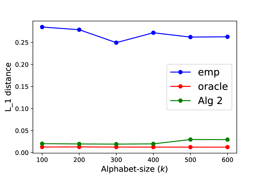
(a) Support size $k$

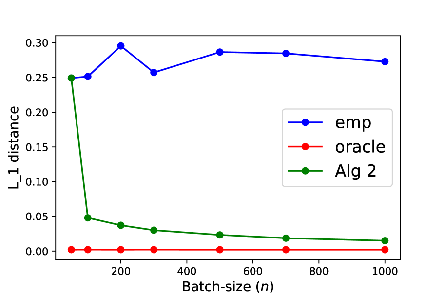
(b) Batch size $n$

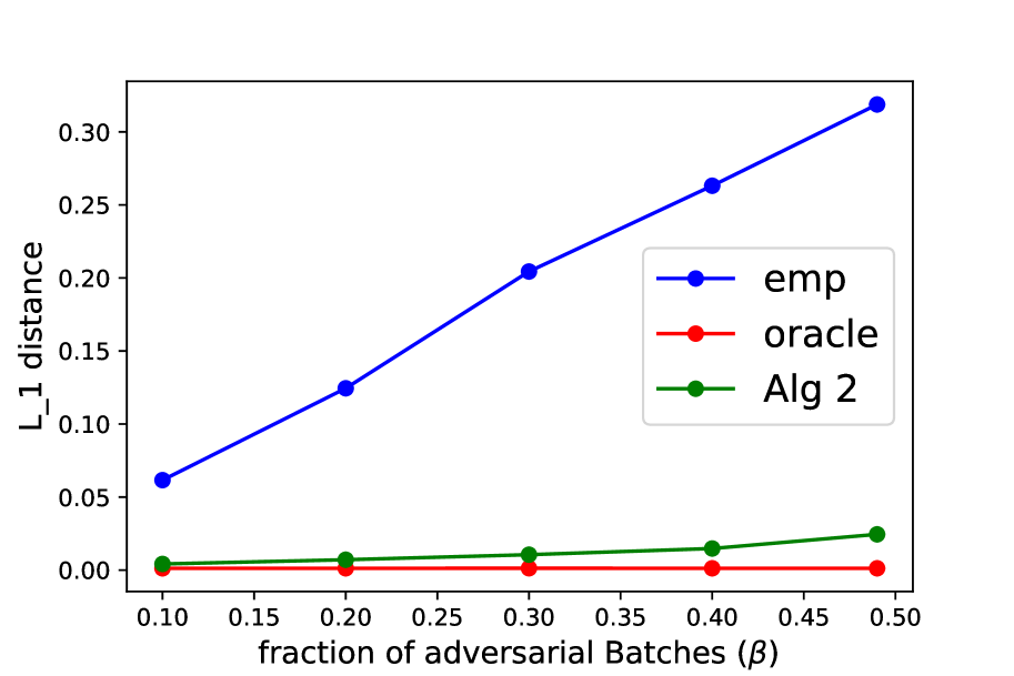
(c) Adversarial batches fraction $\beta$

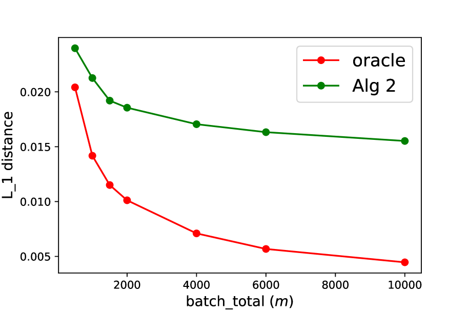
(d) Number of batches $m$

Figure 1: $L_{1}$ estimation error with different Parameters

All experiments were performed on a laptop with a configuration of 2.3 GHz Intel Core i7 CPU and 16 GB of RAM. We choose the parameters for the algorithm by using a small simulation. We provide all codes and implementation details in the supplementary material.

We show four plots here. In each plot we vary one parameter and plot the $L_{1}$ loss incurred by all three estimators. For each experiment, we ran ten trials and reported the average $L_{1}$ distance achieved by each estimator.

For the first plot we fix batch-size $n=1000$ and $\beta=0.4$ and vary alphabet size $k$. We generate $m=k/(0.4)^{2}$ batches for each $k$. Our algorithm’s performance show no significant change as the size of alphabet increases and its performance nearly matches the performance of the Oracle and outperforms the naive estimator by order of magnitudes.

In the the second plot we fix $\beta=0.4$ and $k=200$ and vary batch size $n$. We choose $m=40\times\frac{k}{\beta^{2}}\times\frac{1000}{n}$, this keeps the total number of samples $n\times m$, constant for different $n$. We see that the $L_{1}$ loss incurred by our estimator is much smaller than the naive empirical estimator and it diminishes as the batch size increases and comes very close to the performance of the oracle. Note that this roughly matches the decay $O(1/\sqrt{n})$ of $L_{1}$ error characterized in both the lower and the upper bounds.

For the next plot we fix batch size $n=1000$ and $k=200$. The number of good batches $(1-\beta)m=400k$ is kept same. We vary the adversarial noise level and plot the performance of all estimators. We tested our estimator for fraction of adversarial batches as high as $0.49$ and still our estimator recovered $p$ to a good accuracy and in fact at the lower noise level it is essentially similar to the oracle and it increases (near) linearly with the noise level $\beta$ as in Theorem 1,

In the last plot we fixed all other parameters $n=1000$, $k=200$, and $\beta=0.4$ and varied the number of batches. We see that the performance of oracle keep improving as number of bathes increases. But for our algorithm it decreases initially but later it saturates as predicted by adversarial batch lower bound.

Appendix A Proof of Lemma  3

In this section, we show that conditions 1-3 holds with high probability and prove Lemma 3. To prove the lemma we first prove three auxiliary lemmas; each of these three Lemma will lead to one of the three conditions in Lemma 3. These three lemmas characterizes the statistical properties of the collection of good batches ${B}_{G}$. We state and prove these lemmas in the next subsection.

A.1 Statistical Properties of the Good Batches

Recall that, for a good batch $b\in{B}_{G}$ and subset $S\subseteq[k]$, $\mathbf{1}_{S}(X_{i}^{b})$, for $i\in[n]$, are i.i.d. indicator random variables and ${\bar{\mu}_{b}(S)}$ is the mean of these $n$ indicator variables. Since the indicator random variables are sub-gaussian, namely $\mathbf{1}_{S}(X_{i}^{b})\sim\text{subG}(p(S),1/4)$, the mean ${\bar{\mu}_{b}(S)}$ satisfies ${\bar{\mu}_{b}(S)}\sim\text{subG}(p(S),1/4n)$. $\text{subG}(.)$ is used to denote a sub-gaussian distribution. This observation plays the key role in the proof of all three auxiliary lemmas in this section.

The first lemma among these three lemma show that for any fixed subset $S\subseteq[k]$, ${\bar{\mu}_{b}(S)}$ for most of the good batches is close to $p(S)$. This lemma is used to show Condition 1.

Lemma 10.

For any $\epsilon\in(0,1/4]$ and $|{{B}_{G}}|\geq 12k/\epsilon$, $\forall\,S\subseteq[k]$, with probability $\geq 1-e^{-k}$,

$$\big{|}\big{\{}b\in{B}_{G}:|{\bar{\mu}_{b}(S)}-p(S)|\geq\sqrt{\frac{\ln(1/\epsilon)}{n}}\big{\}}\big{|}\leq\epsilon|{{B}_{G}}|.$$

Proof.

From Hoeffding’s inequality, for $b\in{B}_{G}$ and $S\subseteq[k]$,

$$\Pr\Big{[}|{\bar{\mu}_{b}(S)}-p(S)|\geq{\sqrt{\frac{\ln(1/\epsilon)}{n}}}\Big{]}\leq 2e^{-2\ln(1/\epsilon)}\leq 2{\epsilon}^{2}\leq\epsilon/2.$$

Let $\mathbbm{1}_{b}(S)$ be the indicator random variable that takes the value 1 iff $|{\bar{\mu}_{b}(S)}-p(S)|\geq\sqrt{\ln(1/\epsilon)/n}$. Therefore, for $b\in{B}_{G}$, $E[\mathbbm{1}_{b}(S)]\leq\epsilon/2$. Using the Chernoff bound,

$$\Pr[\sum_{b\in{B}_{G}}\mathbbm{1}_{b}(S)\geq{\epsilon}|{{B}_{G}}|]\leq e^{-\frac{1}{3}\cdot\frac{\epsilon}{2}|{{B}_{G}}|}\leq e^{-2k}.$$

Taking the union bound over all $2^{k}$ subsets $S$ completes the proof. ∎

The next lemma show that even upon removal of any small fraction of good batches from ${B}_{G}$, the empirical mean and the variance of the remaining sub-collection of batches approximate the distribution mean and the variance well enough.

Lemma 11.

For any $\epsilon\in(0,1/4]$, and $|{{B}_{G}}|\geq\frac{k}{\epsilon^{2}\ln(e/\epsilon)}$. Then $\forall\,S\subseteq[k]$ and $\forall\,{B}^{\prime}_{G}\subseteq{B}_{G}$ of size $|{B}^{\prime}_{G}|\geq(1-\epsilon)|{{B}_{G}}|$, with probability $\geq 1-6e^{-k}$,

$$\Big{|}{\bar{p}_{{B}^{\prime}_{G}}(S)}-p(S)|\leq 3\epsilon\sqrt{\frac{\ln(e/\epsilon)}{n}}$$ (2)

and

$$\Big{|}\frac{1}{|{B}^{\prime}_{G}|}\sum_{b\in{B}^{\prime}_{G}}({\bar{\mu}_{b}(S)}-p(S))^{2}-\text{V}(p(S))\Big{|}\leq 32{\frac{\epsilon\ln(e/\epsilon)}{n}}.$$ (3)

Proof.

From Hoeffding’s inequality,

$$\Pr\Big{[}|{{B}_{G}}||\bar{p}_{{B}_{G}}(S)-p(S)|\geq|{{B}_{G}}|{\epsilon} \sqrt{\frac{\ln(e/\epsilon)}{n}}\Big{]}=\Pr\Big{[}\big{|}\sum_{b\in{B}_{G}}({\bar{\mu}_{b}(S)}-p(S))\big{|}\geq|{{B}_{G}}|{\epsilon}\sqrt{\frac{\ln(e/\epsilon)}{n}}\Big{]}$$

$$\leq 2e^{-\frac{|{{B}_{G}}|\epsilon^{2}}{2/(4n)}\cdot{\frac{\ln(e/\epsilon)}{n}}}=2e^{-{2|{{B}_{G}}|\epsilon^{2}}\ln(e/\epsilon)}\leq 2e^{-2k}.$$ (4)

Similarly, for a fix sub-collection $U_{G}\subseteq{B}_{G}$ of size $1\leq|U_{G}|\leq\epsilon|{{B}_{G}}|$,

$$\Pr\Big{[}|U_{G}|\cdot|\bar{p}_{U_{G}}(S)-p(S)|\geq{\epsilon|{{B}_{G}}|}\sqrt{\frac{\ln(e/\epsilon)}{n}}\Big{]} =\Pr\Big{[}\Big{|}\sum_{b\in U_{G}}({\bar{\mu}_{b}(S)}-p(S))\Big{|}\geq{\epsilon|{{B}_{G}}|}\sqrt{\frac{\ln(e/\epsilon)}{n}}\Big{]}$$

$$\leq 2e^{-2\ln(e/\epsilon)\frac{(\epsilon|{{B}_{G}}|)^{2}}{|U_{G}|}}\leq 2e^{-2\epsilon|{{B}_{G}}|\ln(e/\epsilon)},$$

where the last inequality used $|U_{G}|\leq\epsilon|{{B}_{G}}|$. Next, the number of sub-collections (non-empty) of ${B}_{G}$ with size $\leq\epsilon|{{B}_{G}}|$ is bounded by

$$\sum_{j=1}^{\lfloor\epsilon|{{B}_{G}}|\rfloor}{|{{B}_{G}}|\choose j}\leq\epsilon|{{B}_{G}}|{|{{B}_{G}}|\choose{\lfloor\epsilon|{{B}_{G}}|\rfloor}}\leq\epsilon|{{B}_{G}}|\Big{(}\frac{e|{{B}_{G}}|}{\epsilon|{{B}_{G}}|}\Big{)}^{\epsilon|{{B}_{G}}|}\leq e^{\epsilon|{{B}_{G}}|\ln(e/\epsilon)+\ln(\epsilon|{{B}_{G}}|)}<e^{\frac{3}{2}\epsilon|{{B}_{G}}|\ln(e/\epsilon)},$$ (5)

where last of the above inequality used ${\ln(\epsilon|{{B}_{G}}|)}<{\epsilon|{{B}_{G}}|}/2$ and $\ln(e/\epsilon)\geq 1$. Then, using the union bound, $\forall\ U_{G}\subseteq{B}_{G}$ such that $|U_{G}|\leq\epsilon|{{B}_{G}}|$, we get

$$\Pr\Big{[}|U_{G}|\cdot|\bar{p}_{U_{G}}(S)-p(S)|\geq{\epsilon|{{B}_{G}}|}\sqrt{\frac{\ln(e/\epsilon)}{n}}\Big{]}\leq 2e^{-\frac{1}{2}\epsilon|{{B}_{G}}|\ln(e/\epsilon)}<2e^{-\frac{k}{2\epsilon}}<2e^{-2k}.$$ (6)

For any sub-collection ${B}^{\prime}_{G}\subseteq{B}_{G}$ with $|{B}^{\prime}_{G}|\geq(1-\epsilon)|{{B}_{G}}|$,

$$|\sum_{b\in{B}^{\prime}_{G}}({\bar{\mu}_{b}(S)}-p(S))| =|\sum_{b\in{B}_{G}}({\bar{\mu}_{b}(S)}-p(S))-\sum_{b\in{B}_{G}/{B}^{\prime}_{G}}({\bar{\mu}_{b}(S)}-p(S))|$$

$$\leq\Big{|}\sum_{b\in{B}_{G}}({\bar{\mu}_{b}(S)}-p(S))\Big{|}+\Big{|}\sum_{b\in{B}_{G}/{B}^{\prime}_{G}}({\bar{\mu}_{b}(S)}-p(S))\Big{|}$$

$$\leq|{{B}_{G}}|\times|\bar{p}_{{B}_{G}}(S)-p(S)|+\max_{U_{G}:|U_{G}|\leq\epsilon|{{B}_{G}}|}|U_{G}|\times|\bar{p}_{U_{G}}(S)-p(S)|$$

$$\leq{2\epsilon|{{B}_{G}}|}\sqrt{\frac{\ln(e/\epsilon)}{n}},$$

with probability $\geq 1-2e^{-2k}-2e^{-2k}\geq 1-4e^{-2k}$. Then

$$|{\bar{p}_{{B}^{\prime}_{G}}(S)}-p(S)| =\frac{1}{|{B}^{\prime}_{G}|}\Big{|}\sum_{b\in{B}^{\prime}_{G}}({\bar{\mu}_{b}(S)}-p(S))\Big{|}\leq 2\frac{\epsilon|{{B}_{G}}|}{|{B}^{\prime}_{G}|}\sqrt{\frac{\ln(e/\epsilon)}{n}}$$

$$\leq\frac{2\epsilon}{(1-\epsilon)}\sqrt{\frac{\ln(e/\epsilon)}{n}}<{3\epsilon}\sqrt{\frac{\ln(e/\epsilon)}{n}},$$

with probability $\geq 1-4e^{-2k}$. The last step used $\epsilon\leq 1/4$. Since there are $2^{k}$ different choices for $S\subseteq[k]$, from the union bound we get,

$$\Pr\Big{[}\bigcup_{S\subseteq[k]}\Big{\{}|{\bar{p}_{{B}^{\prime}_{G}}(S)}-p(S)|>{4\epsilon}\sqrt{\frac{\ln(e/\epsilon)}{n}}\Big{\}}\Big{]}\leq 4e^{-2k}\times 2^{k}=4e^{-k}.$$

This completes the proof of (2).

Let $Y_{b}=({\bar{\mu}_{b}(S)}-p(S))^{2}-\text{V}(p(S))$. For $b\in{B}_{G}$, ${\bar{\mu}_{b}(S)}-p(S)\sim\text{subG}(1/4n)$, therefore

$$({\bar{\mu}_{b}(S)}-p(S))^{2}-E({\bar{\mu}_{b}(S)}-p(S))^{2}=Y_{b}\sim\text{subE}(\frac{16}{4n})=\text{subE}(\frac{4}{n}).$$

Here subE is sub exponential distribution [Phi15]. Then Bernstein’s inequality gives:

$$\Pr[\Big{|}\sum_{b\in{B}_{G}}Y_{b}\Big{|}\geq 8|{{B}_{G}}|\frac{\epsilon}{{n}}\ln(e/\epsilon)]\leq 2e^{-\frac{|{{B}_{G}}|}{2}\big{(}\frac{8\epsilon\ln(e/\epsilon)/n}{4/n}\big{)}^{2}}=2e^{-2{|{{B}_{G}}|}\epsilon^{2}\ln^{2}(e/\epsilon)}\leq 2e^{-2k}.$$

Next, for a fix sub-collection $U_{G}\subseteq{B}_{G}$ of size $1\leq|U_{G}|\leq\epsilon|{{B}_{G}}|$,

$$\Pr\Big{[}\Big{|}\sum_{b\in U_{G}}Y_{b}\Big{|}\geq 16{\epsilon|{{B}_{G}}|}{\frac{\ln(e/\epsilon)}{n}}\Big{]} \leq 2e^{-\frac{16{\epsilon|{{B}_{G}}|}{\frac{\ln(e/\epsilon)}{n}}}{2\times 4/n}}$$

$$\leq 2e^{-2\epsilon|{{B}_{G}}|\ln(e/\epsilon)}.$$

Then following the same steps as in the proof of (2) one can complete the proof of (3). ∎

To state the next lemma, we make use of the following definition. For a subset $S\subseteq[k]$, let

$${B}_{G}^{d}(S,\epsilon)\triangleq\big{\{}b\in{B}_{G}:|{\bar{\mu}_{b}(S)}-p(S)|\geq 2\sqrt{\frac{\ln(6e/\epsilon)}{n}})\big{\}}$$

be the sub-collection of batches for which empirical probabilities ${\bar{\mu}_{b}(S)}$ are far from $p(S)$ for a given set $S$.

The last lemma of the section upper bounds the total squared deviation of empirical probabilities ${\bar{\mu}_{b}(S)}$ from $p(S)$ for batches in sub-collection ${B}_{G}^{d}(S,\epsilon)$. It helps in upper bounding the corruption for good batches and show that Condition 3 holds with high probability.

Lemma 12.

For any $0<\epsilon<1/2$, and $|{{B}_{G}}|\geq\frac{120k}{\epsilon\ln(e/\epsilon)}$. Then $\forall\,S\subseteq[k]$, with probability $\geq 1-2e^{-k}$,

$$|{B}_{G}^{d}(S,\epsilon)|\leq\frac{\epsilon}{40}|{{B}_{G}}|,$$ (7)

and

$$\sum_{b\in{B}_{G}^{d}(S,\epsilon)}({\bar{\mu}_{b}(S)}-p(S))^{2}<\frac{\epsilon}{2}|{{B}_{G}}|{\frac{\ln(e/\epsilon)}{n}}.$$ (8)

Proof.

The proof of the first part is the same as (with different constants) Lemma 10 and we skip it to avoid repetition.

To prove the second part we bound the total squared deviation of any subset of size $\leq\frac{\epsilon}{40}|{{B}_{G}}|$.

Let $Y_{b}=({\bar{\mu}_{b}(S)}-p(S))^{2}-\text{V}(p(S))$. Similar to the previous lemma, for a fix sub-collection $U_{G}\subseteq{B}_{G}$ of size $1\leq|U_{G}|\leq\frac{\epsilon}{40}|{{B}_{G}}|$, Bernstein’s inequality gives:

$$\Pr\Big{[}\Big{|}\sum_{b\in U_{G}}Y_{b}\Big{|}\geq 8{\frac{\epsilon}{20}|{{B}_{G}}|}{\frac{\ln(e/\epsilon)}{n}}\Big{]} \leq 2e^{-\frac{8{\epsilon|{{B}_{G}}|}{\frac{\ln(e/\epsilon)}{n}}}{20\times 2\times 4/n}}$$

$$\leq 2e^{-\frac{\epsilon}{20}|{{B}_{G}}|\ln(e/\epsilon)}.$$

From (5), there are $e^{\frac{3}{80}\epsilon|{{B}_{G}}|\ln(e/\epsilon)}$ many sub-collections of size $\leq\frac{\epsilon}{40}|{{B}_{G}}|$. Then taking the union bound for all sub-collections of this size and all subsets $S\subseteq[k]$ we get,

$$\Big{|}\sum_{b\in U_{G}}\Big{(}({\bar{\mu}_{b}(S)}-p(S))^{2}-\text{V}(p(S))\Big{)}\Big{|}\leq{\frac{2\epsilon}{5}|{{B}_{G}}|}{\frac{\ln(e/\epsilon)}{n}},$$

for all $U_{G}$ of size $\leq\frac{\epsilon}{40}|{{B}_{G}}|$. Then using the fact that $\text{V}(.)$ is upper bounded by $\frac{1}{4n}$, and therefore $|U_{G}|\text{V}(p(S))\leq\frac{\epsilon}{4\times 40}|{{B}_{G}}|$, completes the proof. ∎

A.2 Completing the proof of Lemma 3

We first show condition 1 holds with high probability.

It is easy to verify that $|p(S)-\text{med}(\bar{\mu}(S))|\geq\sqrt{\ln 6/n}$, only if the sub-collection $T=\{b:|p(S)-{\bar{\mu}_{b}(S)}|\geq\sqrt{\ln 6/n}\}$ has at-least $0.5m$ batches. But

$$|T|=|T\cap{B}_{G}|+|T\cap{B}_{A}|\overset{\text{(a)}}{<}|{B}_{G}|/6+|{B}_{A}|=\frac{m}{6}+\frac{5}{6}|{B}_{A}|\overset{\text{(b)}}{\leq}\frac{m}{6}+\frac{2m}{6}=0.5m,$$

where inequality (a) follows from Lemma 10 by choosing $\epsilon=1/6$ and (b) follows since $|{{B}_{A}}|\leq\beta m\leq 0.4m$.

Using $\epsilon=\beta/6$ in Lemma 11 gives Condition 2.

Finally, we show the last condition. To show it we use $\epsilon=\beta$ in Lemma 12. From Condition 1, note that for $b\in{B}_{G}\setminus{B}_{G}^{d}(S,\beta)$

$$|{\bar{\mu}_{b}(S)}-\text{med}(\bar{\mu}(S))|\leq|{\bar{\mu}_{b}(S)}-p(S)|+|p(S)-\text{med}(\bar{\mu}(S))|\leq 2\sqrt{\frac{\ln(6e/\beta)}{n}}+\sqrt{\frac{\ln 6}{n}}\leq 3\sqrt{\frac{\ln(6e/\beta)}{n}},$$

Then, for $b\in{B}_{G}\setminus{B}_{G}^{d}(S,\beta)$, from the definition of corruption score it follows that $\psi_{b}(S)=0$. Next set of inequalities complete the proof of condition 3.

$$\psi({B}_{G}) =\sum_{b\in{B}_{G}}\psi_{b}(S)=\sum_{b\in{B}_{G}\setminus{B}_{G}^{d}(S,\beta)}\psi_{b}(S)+\sum_{b\in{B}_{G}^{d}(S,\beta)}\psi_{b}(S)$$

$$=\sum_{b\in{B}_{G}^{d}(S,\beta)}\psi_{b}(S)$$

$$\overset{\text{(a)}}{\leq}\sum_{b\in{B}_{G}^{d}(S,\beta)}({\bar{\mu}_{b}(S)}-\text{med}(\bar{\mu}(S)))^{2}$$

$$=\sum_{b\in{B}_{G}^{d}(S,\beta)}({\bar{\mu}_{b}(S)}-p(S)+p(S)-\text{med}(\bar{\mu}(S)))^{2}$$

$$\overset{\text{(b)}}{\leq}\sum_{b\in{B}_{G}^{d}(S,\beta)}({\bar{\mu}_{b}(S)}-p(S))^{2}+\sum_{b\in{B}_{G}^{d}(S,\beta)}(\text{med}(\bar{\mu}(S))-p(S))^{2}$$

$$+2\sqrt{\Bigg{(}\sum_{b\in{B}_{G}^{d}(S,\beta)}({\bar{\mu}_{b}(S)}-p(S))^{2}\Bigg{)}\Bigg{(}\sum_{b\in{B}_{G}^{d}(S,\beta)}(\text{med}(\bar{\mu}(S))-p(S))^{2}\Bigg{)}}$$

$$\overset{\text{(c)}}{\leq}\frac{\beta}{2}|{{B}_{G}}|{\frac{\ln(e/\beta)}{n}}+\frac{\beta}{40}|{{B}_{G}}|{\frac{\ln 6}{n}}+\sqrt{\frac{\beta}{2}|{{B}_{G}}|{\frac{\ln(e/\beta)}{n}}\times\frac{\beta}{40}|{{B}_{G}}|{\frac{\ln 6}{n}}}<{\beta}|{{B}_{G}}|{\frac{\ln(e/\beta)}{n}},$$

here (a) follows from the definition of the corruption score, (b) uses Cauchy-Schwarz inequality and (c) follows from Lemma 12 and Condition 1.

Appendix B Proof of the other Lemmas

We first prove an auxiliary Lemma that will be useful in other proofs. For a given sub-collection ${B}^{\prime}$ and subset $S$, the next lemma bounds the total squared distance of ${\bar{\mu}_{b}(S)}$ from $p(S)$ for adversarial batches in ${B}^{\prime}$ in terms of corruption score $\psi({B}^{\prime},S)$.

Lemma 13.

Suppose the conditions 1 and 3 holds. For subset $S$, let $\psi({B}^{\prime},S)=t\cdot\kappa_{G}$, for some $t\geq 0$, then

$$(t-3-2\sqrt{t})\kappa_{G}\leq\sum_{b\in{B}^{\prime}\cap{B}_{A}}({\bar{\mu}_{b}(S)}-p(S))^{2}\leq(t+17+2\sqrt{t})\kappa_{G}.$$

Proof.

For the purpose of this proof, let ${B}^{\prime}_{G}={B}^{\prime}\cap{B}_{G}$ and ${B}^{\prime}_{A}={B}^{\prime}\cap{B}_{A}$. Then

$$\sum_{b\in{B}^{\prime}_{A}}({\bar{\mu}_{b}(S)}-p(S))^{2}=\sum_{b\in{B}^{\prime}_{A}:\psi_{b}(S)>0}({\bar{\mu}_{b}(S)}-p(S))^{2}+\sum_{b\in{B}^{\prime}_{A}:\psi_{b}(S)=0}({\bar{\mu}_{b}(S)}-p(S))^{2}$$ (9)

From the definition of corruption score, for batch $b\in{B}^{\prime}$, with zero corruption score $\psi_{b}(S)$, we have $|{\bar{\mu}_{b}(S)}-\text{med}(\bar{\mu}(S))|\leq 3\sqrt{\frac{\ln(6e/\beta)}{n}}$. Then using Condition 1 and the triangle inequality, for such batches with zero corruption score, we get

$$|{\bar{\mu}_{b}(S)}-p(S)|\leq\sqrt{\ln(6)/n}+3\sqrt{\frac{\ln(6e/\beta)}{n}}<4\sqrt{\frac{\ln(6e/\beta)}{n}}.$$ (10)

Next,

$$\sum_{b\in{B}^{\prime}_{A}:\psi_{b}(S)>0}({\bar{\mu}_{b}(S)}-p(S))^{2}$$

$$=\sum_{b\in{B}^{\prime}_{A}:\psi_{b}(S)>0}({\bar{\mu}_{b}(S)}-\text{med}(\bar{\mu}(S))+\text{med}(\bar{\mu}(S))-p(S))^{2}$$

$$\overset{\text{(a)}}{\leq}\sum_{b\in{B}^{\prime}_{A}:\psi_{b}(S)>0}({\bar{\mu}_{b}(S)}-\text{med}(\bar{\mu}(S)))^{2}+\sum_{b\in{B}^{\prime}_{A}:\psi_{b}(S)>0}(\text{med}(\bar{\mu}(S))-p(S))^{2}$$

$$+2\sqrt{\Bigg{(}\sum_{b\in{B}^{\prime}_{A}:\psi_{b}(S)>0}({\bar{\mu}_{b}(S)}-\text{med}(\bar{\mu}(S)))^{2}\Bigg{)}\Bigg{(}\sum_{b\in{B}^{\prime}_{A}:\psi_{b}(S)>0}(\text{med}(\bar{\mu}(S))-p(S))^{2}\Bigg{)}}$$

$$\overset{\text{(b)}}{\leq}\sum_{b\in{B}^{\prime}_{A}}\psi_{b}(S)+\sum_{b\in{B}^{\prime}_{A}}\frac{\ln 6}{n}+2\sqrt{\Bigg{(}\sum_{b\in{B}^{\prime}_{A}}\psi_{b}(S)\Bigg{)}\Bigg{(}\sum_{b\in{B}^{\prime}_{A}}\frac{\ln 6}{n}\Bigg{)}}$$

$$\overset{\text{(c)}}{\leq}\psi({B}^{\prime}_{A},S)+\kappa_{G}+2\sqrt{\psi({B}^{\prime}_{A},S)\cdot\kappa_{G}},$$ (11)

here (a) uses Cauchy-Schwarz inequality, (b) follows from the definition of corruption score and Condition 1, and (c) uses $|{B}^{\prime}_{A}|\leq\beta m$ and $(\beta m\ln 6)/n\leq\kappa_{G}$.

A similar calculation as the above leads to the following

$$\sum_{b\in{B}^{\prime}_{A}:\psi_{b}(S)>0}({\bar{\mu}_{b}(S)}-p(S))^{2}\geq\psi({B}^{\prime}_{A},S)-2\sqrt{\psi({B}^{\prime}_{A},S)\cdot\kappa_{G}},$$ (12)

Next, we show the upper bound in the lemma. Combining equations (9), (10) and (11) gives

$$\sum_{b\in{B}^{\prime}_{A}}({\bar{\mu}_{b}(S)}-p(S))^{2} \leq\psi({B}^{\prime}_{A},S)+\kappa_{G}+2\sqrt{\psi({B}^{\prime}_{A},S)\cdot\kappa_{G}}+\sum_{b\in{B}^{\prime}_{A}:\psi_{b}(S)=0}4\sqrt{{\frac{\ln(6e/\beta)}{n}}}$$

$$\leq\psi({B}^{\prime},S)+\kappa_{G}+2\sqrt{\psi({B}^{\prime},S)\cdot\kappa_{G}}+16|{B}_{A}|{\frac{\ln(6e/\beta)}{n}}$$

$$\leq(t+17+2\sqrt{t})\kappa_{G},$$

here the second last inequality used ${B}^{\prime}_{A}\subseteq{B}^{\prime}$ and ${B}^{\prime}_{A}\subseteq{B}_{A}$. This completes the proof of the upper bound.

To prove the lower bound, we first note that

$$\psi({B}^{\prime},S)=\sum_{b\in{B}^{\prime}}\psi_{b}(S)=\sum_{b\in{B}^{\prime}_{G}}\psi_{b}(S)+\sum_{b\in{B}^{\prime}_{A}}\psi_{b}(S)$$

$$\leq\sum_{b\in{B}_{G}}\psi_{b}(S)+\psi({B}^{\prime}_{A},S)$$

$$\leq\psi({B}_{G})+\psi({B}^{\prime}_{A},S)\leq{\frac{\beta m\ln({6e}/\beta)}{n}}+\sum_{b\in{B}^{\prime}_{A}}\psi_{b}(S),$$

here the last inequality uses condition 3. The above equation implies that

$$\psi({B}^{\prime}_{A},S)\geq\psi({B}^{\prime},S)-\beta m{\frac{\ln(6e/\beta)}{n}}=(t-1)\kappa_{G}.$$ (13)

By combining, equations (9) (12) and (13), we get the lower bound

$$\sum_{b\in{B}^{\prime}_{A}}({\bar{\mu}_{b}(S)}-p(S))^{2} \geq(t-1)\kappa_{G}-2\sqrt{|t-1|\kappa_{G}\cdot\kappa_{G}}=(t-1-2\sqrt{|t-1|})\kappa_{G}\geq(t-3-2\sqrt{t})\kappa_{G}.$$

∎

B.1 Proof of Lemma 4

Proof.

For the purpose of this proof, let ${B}^{\prime}_{G}={B}^{\prime}\cap{B}_{G}$ and ${B}^{\prime}_{A}={B}^{\prime}\cap{B}_{A}$. Note that $|{B}^{\prime}|\geq|{B}^{\prime}_{G}|\geq(1-\beta/6){B}_{G}$.

Fix subset $S\subseteq[k]$. Next,

$${\bar{p}_{{B}^{\prime}}(S)}-p(S)=\frac{1}{|{B}^{\prime}|}\sum_{b\in{B}^{\prime}}{\bar{\mu}_{b}(S)}-p(S)=\frac{1}{|{B}^{\prime}|}\sum_{b\in{B}^{\prime}}({\bar{\mu}_{b}(S)}-p(S))$$

$$=\frac{1}{|{B}^{\prime}|}\sum_{b\in{B}^{\prime}_{G}}({\bar{\mu}_{b}(S)}-p(S))+\frac{1}{|{B}^{\prime}|}\sum_{b\in{B}^{\prime}_{A}}({\bar{\mu}_{b}(S)}-p(S))$$

$$=\frac{|{B}^{\prime}_{G}|}{|{B}^{\prime}|}({\bar{p}_{{B}^{\prime}_{G}}(S)}-p(S))+\frac{1}{|{B}^{\prime}|}\sum_{b\in{B}^{\prime}_{A}}({\bar{\mu}_{b}(S)}-p(S))$$

Therefore,

$$|{\bar{p}_{{B}^{\prime}}(S)}-p(S)| \leq\frac{|{B}^{\prime}_{G}|}{|{B}^{\prime}|}|{\bar{p}_{{B}^{\prime}_{G}}(S)}-p(S)|+\frac{1}{|{B}^{\prime}|}\sum_{b\in{B}^{\prime}_{A}}|{\bar{\mu}_{b}(S)}-p(S)|$$

$$\overset{\text{(a)}}{\leq}\frac{\beta}{2}\sqrt{\frac{\ln(6e/\beta)}{n}}+\frac{1}{|{B}^{\prime}|}\sum_{b\in{B}^{\prime}_{A}}|{\bar{\mu}_{b}(S)}-p(S)|$$

$$\overset{\text{(b)}}{\leq}\frac{\beta}{2}\sqrt{\frac{\ln(6e/\beta)}{n}}+\frac{1}{|{B}^{\prime}|}\sqrt{|{B}^{\prime}_{A}|\sum_{b\in{B}^{\prime}_{A}}({\bar{\mu}_{b}(S)}-p(S))^{2}}$$

$$\overset{\text{(c)}}{\leq}\frac{\beta}{2}\sqrt{\frac{\ln(6e/\beta)}{n}}+\frac{1}{|{B}^{\prime}|}\sqrt{|{B}^{\prime}_{A}|\cdot(t+17+2\sqrt{t})\kappa_{G}}$$

$$\overset{\text{(d)}}{\leq}\frac{\beta}{2}\sqrt{\frac{\ln(6e/\beta)}{n}}+\frac{1}{|{B}^{\prime}|}\sqrt{|{B}^{\prime}_{A}|\cdot(t+17+2\sqrt{t})\frac{\beta m\ln({6e}/\beta)}{n}}$$

$$\leq\frac{\beta}{2}\sqrt{\frac{\ln(6e/\beta)}{n}}+\sqrt{\frac{|{B}^{\prime}_{A}|\cdot m}{|{B}^{\prime}|^{2}}\cdot(t+17+2\sqrt{t})\frac{\beta\ln({6e}/\beta)}{n}},$$ (14)

here in (a) uses Condition 2 and $|{B}^{\prime}_{G}|\leq|{B}^{\prime}|$, inequality (b) follows from the Cauchy-Schwarz inequality, inequality (c) uses Lemma 13, and (d) uses the definition of $\kappa_{G}$. Let $|{B}^{\prime}_{A}|=|{B}_{A}|-\text{D}$, for some $\text{D}\in[0,|{B}_{A}|]$. Also from Lemma note that

$$|{B}^{\prime}_{G}|\geq(1-\beta/6)|{{B}_{G}}|=|{{B}_{G}}|-|{{B}_{G}}|\beta/6=|{{B}_{G}}|-m\beta(1-\beta)/6.$$

Therefore,

$$\frac{|{B}^{\prime}_{A}|\cdot m}{|{B}^{\prime}|^{2}}=\frac{|{B}^{\prime}_{A}|\cdot m}{(|{B}^{\prime}_{A}|+|{B}^{\prime}_{G}|)^{2}} \leq\frac{(|{B}_{A}|-\text{D})m}{(|{B}_{A}|-\text{D}+|{{B}_{G}}|-m\beta(1-\beta)/6)^{2}}$$

$$=\frac{(\beta m-\text{D})m}{(m-\text{D}-m\beta(1-\beta)/6)^{2}}$$

$$\overset{\text{(a)}}{\leq}\frac{(\beta m-\text{D})m}{(m-\text{D}-0.04m)^{2}}$$

$$\overset{\text{(b)}}{\leq}\frac{\beta m^{2}}{(0.96m)^{2}}\leq\frac{\beta}{0.96^{2}},$$

here (a) follows since $\beta(1-\beta)$ takes maximum value at $\beta=0.4$ in range $\beta\in(0,0.4]$, and (b) follows since the expression is maximized at $\text{D}=0$.

Then combining above equation with (14) gives

$$|{\bar{p}_{{B}^{\prime}}(S)}-p(S)| \leq\frac{\beta}{2}\sqrt{\frac{\ln(6e/\beta)}{n}}+\sqrt{(t+17+2\sqrt{t})\frac{\beta^{2}\ln({6e}/\beta)}{0.96^{2}n}}$$

$$\leq\Big{(}1/2+\frac{1}{0.96}\sqrt{(t+17+2\sqrt{t})}\Big{)}\beta\sqrt{\frac{\ln(6e/\beta)}{n}}$$ (15)

$$\overset{\text{(a)}}{\leq}\Big{(}5+\sqrt{2.1t}\Big{)}\beta\sqrt{\frac{\ln(6e/\beta)}{n}},$$ (16)

here inequality (a) uses the fact that $2t^{1/2}\leq t+1$ and $\sqrt{x^{2}+y^{2}}\leq|x|+|y|$. Finally, using the definition of $L_{1}$ distance between two distributions complete the proof of the Theorem. ∎

B.2 Proof of Lemma 6

Proof.

From the second statement in Lemma 5, each batch that gets removed is adversarial with probability $\geq 0.95$. Batch deletion deletes more than $0.1\beta m$ good batches in total over all runs iff it samples $0.1\beta m$ good batches in first $0.1\beta m+|{B}_{A}|$ batches removed as otherwise all adversarial batches would have been exhausted already and Batch deletion algorithm would not remove batches any further. But the expected number of good batches sampled is $\leq 0.05(\times 0.1\beta m+|{B}_{A}|)\leq 0.005\beta m+0.05\beta m<0.06\beta m$.

Then using the Chernoff-bound, probability of sampling (removing) more than $0.1\beta m$ good batches in $0.1\beta m+|{B}_{A}|$ deletions is $\leq e^{-O(\beta m)}\leq e^{-O(k)}$. Hence, with high probability the algorithm deletes less than $0.1\beta m=0.6\beta m/6\leq|{{B}_{G}}|\beta/6$ batches. ∎

B.3 Proof of Lemma 7

Proof.

For the purpose of this proof, let ${B}^{\prime}_{G}={B}^{\prime}\cap{B}_{G}$ and ${B}^{\prime}_{A}={B}^{\prime}\cap{B}_{A}$. For batches $b$ in a sub-collection ${B}^{\prime}$, the next equation relates the empirical variance of ${\bar{\mu}_{b}(S)}$ to sum of their squared deviation from $p(S)$.

$$|{B}^{\prime}|\overline{\text{V}}_{{B}^{\prime}}(S)=\sum_{b\in{B}^{\prime}}({\bar{\mu}_{b}(S)}-{\bar{p}_{{B}^{\prime}}(S)})^{2}=\sum_{b\in{B}^{\prime}}({\bar{\mu}_{b}(S)}-p(S)-({\bar{p}_{{B}^{\prime}}(S)}-p(S)))^{2}$$

$$=\sum_{b\in{B}^{\prime}}\Big{(}({\bar{\mu}_{b}(S)}-p(S))^{2}+({\bar{p}_{{B}^{\prime}}(S)}-p(S))^{2}-2({\bar{p}_{{B}^{\prime}}(S)}-p(S))({\bar{\mu}_{b}(S)}-p(S))\Big{)}$$

$$=\sum_{b\in{B}^{\prime}}({\bar{\mu}_{b}(S)}-p(S))^{2}+|{B}^{\prime}|({\bar{p}_{{B}^{\prime}}(S)}-p(S))^{2}-2({\bar{p}_{{B}^{\prime}}(S)}-p(S))\sum_{b\in{B}^{\prime}}({\bar{\mu}_{b}(S)}-p(S))$$

$$=\sum_{b\in{B}^{\prime}}({\bar{\mu}_{b}(S)}-p(S))^{2}+|{B}^{\prime}|({\bar{p}_{{B}^{\prime}}(S)}-p(S))^{2}-2({\bar{p}_{{B}^{\prime}}(S)}-p(S))(|{B}^{\prime}|{\bar{p}_{{B}^{\prime}}(S)}-|{B}^{\prime}|p(S))$$

$$=\sum_{b\in{B}^{\prime}}({\bar{\mu}_{b}(S)}-p(S))^{2}-|{B}^{\prime}|({\bar{p}_{{B}^{\prime}}(S)}-p(S))^{2}$$

$$=\sum_{b\in{B}^{\prime}_{A}}({\bar{\mu}_{b}(S)}-p(S))^{2}+\sum_{b\in{B}^{\prime}_{G}}({\bar{\mu}_{b}(S)}-p(S))^{2}-|{B}^{\prime}|(p(S)-{\bar{p}_{{B}^{\prime}}(S)})^{2}.$$ (17)

The next set of inequalities lead to the upper bound in the Lemma.

$$|{B}^{\prime}|(\overline{\text{V}}_{{B}^{\prime}}(S)-\text{V}({\bar{p}_{{B}^{\prime}}(S)}))$$

$$\overset{\text{(a)}}{=}\sum_{b\in{B}^{\prime}_{A}}({\bar{\mu}_{b}(S)}-p(S))^{2}+\sum_{b\in{B}^{\prime}_{G}}({\bar{\mu}_{b}(S)}-p(S))^{2}-|{B}^{\prime}|(p(S)-{\bar{p}_{{B}^{\prime}}(S)})^{2}-|{B}^{\prime}|\text{V}({\bar{p}_{{B}^{\prime}}(S)})$$

$$\overset{\text{(b)}}{\leq}(t+17+2\sqrt{t})\kappa_{G}+|{B}^{\prime}_{G}|\text{V}(p(S))+|{B}^{\prime}_{G}|\frac{6\beta\ln(\frac{6e}{\beta})}{n}-|{B}^{\prime}|\text{V}({\bar{p}_{{B}^{\prime}}(S)})$$

$$\overset{\text{(c)}}{\leq}(t+17+2\sqrt{t})\kappa_{G}+6\beta m{\frac{\ln(6e/\beta)}{n}}+|{B}^{\prime}|\text{V}(p(S))-|{B}^{\prime}|\text{V}({\bar{p}_{{B}^{\prime}}(S)})$$

$$\overset{\text{(d)}}{\leq}(t+23+2\sqrt{t})\kappa_{G}+m\frac{|p(S)-{\bar{p}_{{B}^{\prime}}(S)}|}{n},$$

here inequality (a) follows from (17), (b) follows from Lemma 13 and condition 2, and (c) follows since $|{B}^{\prime}_{G}|\leq|{B}^{\prime}|$ and $\text{V}(\cdot)\geq 0$, and inequality (d) uses (1) and $|{B}^{\prime}|\leq m$. Next, from equation (16) we have,

$$|{\bar{p}_{{B}^{\prime}}(S)}-p(S)|\leq(5+\sqrt{2.1t})\beta\sqrt{{\frac{\ln(6e/\beta)}{n}}}$$

$$=(5+\sqrt{2.1t})\beta\ln(6e/\beta)\sqrt{\frac{1}{n\ln(6e/\beta)}}$$

$$\leq(5+\sqrt{2.1t})\frac{n\kappa_{G}}{m}.$$ (18)

Combining the above two equations gives the upper bound in the Lemma.

Next showing the lower bound,

$$|{B}^{\prime}|(\overline{\text{V}}_{{B}^{\prime}}(S)-\text{V}({\bar{p}_{{B}^{\prime}}(S)}))$$

$$\overset{\text{(a)}}{=}\sum_{b\in{B}^{\prime}_{A}}({\bar{\mu}_{b}(S)}-p(S))^{2}+\sum_{b\in{B}^{\prime}_{G}}({\bar{\mu}_{b}(S)}-p(S))^{2}-|{B}^{\prime}|(p(S)-{\bar{p}_{{B}^{\prime}}(S)})^{2}-|{B}^{\prime}|\text{V}({\bar{p}_{{B}^{\prime}}(S)})$$

$$\overset{\text{(b)}}{\geq}(t-3-2\sqrt{t})\kappa_{G}+|{B}^{\prime}_{G}|\text{V}(p(S))-|{B}^{\prime}_{G}|\frac{6\beta\ln(\frac{6e}{\beta})}{n}-|{B}^{\prime}|(p(S)-{\bar{p}_{{B}^{\prime}}(S)})^{2}-|{B}^{\prime}|\text{V}({\bar{p}_{{B}^{\prime}}(S)})$$

$$\geq(t-9-2\sqrt{t})\kappa_{G}+|{B}^{\prime}_{G}|\text{V}(p(S))-|{B}^{\prime}|(p(S)-{\bar{p}_{{B}^{\prime}}(S)})^{2}-|{B}^{\prime}_{G}|\text{V}({\bar{p}_{{B}^{\prime}}(S)})-|{B}^{\prime}_{A}|\text{V}({\bar{p}_{{B}^{\prime}}(S)})$$

$$\geq(t-9-2\sqrt{t})\kappa_{G}-|{B}^{\prime}_{G}|(\text{V}({\bar{p}_{{B}^{\prime}}(S)})-\text{V}(p(S)))-|{B}^{\prime}|(p(S)-{\bar{p}_{{B}^{\prime}}(S)})^{2}-|{B}^{\prime}_{A}|\text{V}({\bar{p}_{{B}^{\prime}}(S)})$$

$$\overset{\text{(c)}}{\geq}(t-9-2\sqrt{t})\kappa_{G}-|{B}^{\prime}_{G}|\frac{|p(S)-{\bar{p}_{{B}^{\prime}}(S)}|}{n}-\frac{|{B}^{\prime}_{A}|}{4n}-|{B}^{\prime}|(p(S)-{\bar{p}_{{B}^{\prime}}(S)})^{2}$$

$$\geq(t-9-2\sqrt{t})\kappa_{G}-m\frac{|p(S)-{\bar{p}_{{B}^{\prime}}(S)}|}{n}-\frac{\beta m}{4n}-m(p(S)-{\bar{p}_{{B}^{\prime}}(S)})^{2}$$

$$\overset{\text{(d)}}{\geq}(t-15-2\sqrt{t}-\sqrt{2.1t})\kappa_{G}-m(p(S)-{\bar{p}_{{B}^{\prime}}(S)})^{2},$$

here inequality (a) follows from (17), (b) follows from Lemma 13 and condition 2, (c) follows from (1) and $\text{V}(\cdot)\leq\frac{1}{4n}$, and inequality (d) follows from (18).

Next, we bound the last tem in the above equation to complete the proof. From equation (15),

$$(p(S)-{\bar{p}_{{B}^{\prime}}(S)})^{2} \leq\Big{(}1/2+\frac{1}{0.96}\sqrt{(t+17+2\sqrt{t})}\Big{)}^{2}\beta^{2}{\frac{\ln(6e/\beta)}{n}}$$

$$\leq\Big{(}1/4+\frac{1}{0.96^{2}}{(t+17+2\sqrt{t})}+\frac{1}{0.96}\sqrt{(t+17+2\sqrt{t})}\Big{)}\beta\cdot\kappa_{G}$$

$$\overset{\text{(a)}}{\leq}\Big{(}1/4+1.1{(t+17+2\sqrt{t})}+5+\sqrt{2.1t}\Big{)}\beta\cdot\kappa_{G}$$

$$\leq\Big{(}24+1.1t+2.2\sqrt{t}+\sqrt{2.1t}\Big{)}\beta\cdot\kappa_{G}$$

$$\overset{\text{(b)}}{\leq}0.4\Big{(}24+1.1t+2.2\sqrt{t}+\sqrt{2.1t}\Big{)}\kappa_{G},$$

here inequality (a) uses the fact that $2t^{1/2}\leq t+1$ and $\sqrt{x^{2}+y^{2}}\leq|x|+|y|$ and inequality (b) uses $\beta\leq 0.4$. Combining above two equations give us the lower bound in the Lemma. ∎

Appendix C Proof of Theorem 9

First, we restate the statement of the main theorem.

Theorem 14.

Suppose the conditions 1- 3 holds. Then Algorithm 2 runs in polynomial time and with probability $\geq 1-O(e^{-k})$ return a sub-collection ${B}^{\prime}_{f}\subseteq{B}$ such that $|{B}^{\prime}_{f}\cap{B}_{G}|\geq(1-\frac{\beta}{6})|{{B}_{G}}|$ and for $p^{*}={\bar{p}_{{B}^{\prime}_{f}}}$,

$$||p^{*}-p||_{1}\leq 100\beta\sqrt{\frac{\ln(6e/\beta)}{n}}.$$

Proof.

Lemma 6 show that for the sub-collection ${B}^{\prime}_{i}$ at each iteration $i$, $|{B}^{\prime}_{i}\cap{B}_{G}|\geq(1-\frac{\beta}{6})|{{B}_{G}}|$, hence, for sub-collection ${B}^{\prime}_{f}$ returned by the algorithm $|{B}^{\prime}_{f}\cap{B}_{G}|\geq(1-\frac{\beta}{6})|{{B}_{G}}|$, with probability $\geq 1-O(e^{-k})$. This also implies that the total number of deleted batches are $<(1+1/6)\beta m$.

To complete the proof of the above Theorem, we state the following corollary, which is a direct consequence of Lemma 7.

Corollary 15.

Suppose the conditions 1- 3 holds. Then following hold for any ${B}^{\prime}\subseteq{B}$ such that $|{B}^{\prime}\cap{B}_{G}|\geq(1-\frac{\beta}{6})|{{B}_{G}}|$.

1. $|\overline{\text{V}}_{{B}^{\prime}}(S)-\text{V}({\bar{p}_{{B}^{\prime}}(S)})|\geq 75\kappa_{G}$ implies that $\psi({B}^{\prime},S)\geq 25\kappa_{G}$.

2. $|\overline{\text{V}}_{{B}^{\prime}}(S)-\text{V}({\bar{p}_{{B}^{\prime}}(S)})|\leq 150\kappa_{G}$ implies that $\psi({B}^{\prime},S)\leq 900\kappa_{G}$.

In each iteration of Algorithm 2, except the last, ${Detection-Algorithm}$ returns a subset for which the difference between two variance estimate is $\geq 75\kappa_{G}$. The first statement in the above corollary implies that corruption is high for this subset. Batch Deletion removes batches from the sub-collection to reduce the corruption for such subset. From Statement 3 of Lemma 5, in each iteration Batch Deletion removes $\geq 25\kappa_{G}-20\kappa_{G}$ batches. Since the total batches removed are $<7/6\beta m$, this implies that the algorithm runs for at-max $\frac{7\beta m}{6\times 5\kappa_{G}}<n$ iterations.

The algorithm terminates when ${Detection-Algorithm}$ returns a subset for which the difference between two variance estimate is $\leq 75\kappa_{G}$. Then Lemma 8 implies that the difference between two variance estimate is $\leq 150\kappa_{G}$ for all subsets. Then the above corollary shows that corruption for all subsets is $\leq 900\kappa_{G}$. Therefore, $\psi({B}^{\prime})\leq 900\kappa_{G}$. Then Lemma 4 bounds the $L_{1}$ distance. ∎

References

- [AN04] Noga Alon and Assaf Naor. Approximating the cut-norm via grothendieck’s inequality. In Proceedings of the thirty-sixth annual ACM symposium on Theory of computing, pages 72–80. ACM, 2004.
- [BS04] Dietrich Braess and Thomas Sauer. Bernstein polynomials and learning theory. Journal of Approximation Theory, 128(2):187–206, 2004.
- [CLM19] Sitan Chen, Jerry Li, and Ankur Moitra. Efficiently learning structured distributions from untrusted batches. arXiv preprint arXiv:1911.02035, 2019.
- [CSV17] Moses Charikar, Jacob Steinhardt, and Gregory Valiant. Learning from untrusted data. In Proceedings of the 49th Annual ACM SIGACT Symposium on Theory of Computing, pages 47–60. ACM, 2017.
- [DKK+16] Ilias Diakonikolas, Gautam Kamath, Daniel M Kane, Jerry Li, Ankur Moitra, and Alistair Stewart. Robust estimators in high dimensions without the computational intractability. In 2016 IEEE 57th Annual Symposium on Foundations of Computer Science (FOCS), pages 655–664. IEEE, 2016.
- [DKK+17] Ilias Diakonikolas, Gautam Kamath, Daniel M Kane, Jerry Li, Ankur Moitra, and Alistair Stewart. Being robust (in high dimensions) can be practical. In Proceedings of the 34th International Conference on Machine Learning-Volume 70, pages 999–1008. JMLR. org, 2017.
- [DKK+19] Ilias Diakonikolas, Gautam Kamath, Daniel Kane, Jerry Li, Ankur Moitra, and Alistair Stewart. Robust estimators in high-dimensions without the computational intractability. SIAM Journal on Computing, 48(2):742–864, 2019.
- [Hub92] Peter J Huber. Robust estimation of a location parameter. In Breakthroughs in statistics, pages 492–518. Springer, 1992.
- [KOPS15] Sudeep Kamath, Alon Orlitsky, Dheeraj Pichapati, and Ananda Theertha Suresh. On learning distributions from their samples. In Conference on Learning Theory, pages 1066–1100, 2015.
- [LRV16] Kevin A Lai, Anup B Rao, and Santosh Vempala. Agnostic estimation of mean and covariance. In 2016 IEEE 57th Annual Symposium on Foundations of Computer Science (FOCS), pages 665–674. IEEE, 2016.
- [MMR+16] H Brendan McMahan, Eider Moore, Daniel Ramage, Seth Hampson, et al. Communication-efficient learning of deep networks from decentralized data. arXiv preprint arXiv:1602.05629, 2016.
- [MR17] H Brendan McMahan and Daniel Ramage. https://research.google.com/pubs/pub44822.html. 2017.
- [Phi15] Rigollet Philippe. 18.s997 high-dimensional statistics. Massachusetts Institute of Technology: MIT OpenCourseWare, https://ocw.mit.edu. License: Creative Commons BY-NC-SA, 2015.
- [QV17] Mingda Qiao and Gregory Valiant. Learning discrete distributions from untrusted batches. arXiv preprint arXiv:1711.08113, 2017.
- [SCV17] Jacob Steinhardt, Moses Charikar, and Gregory Valiant. Resilience: A criterion for learning in the presence of arbitrary outliers. arXiv preprint arXiv:1703.04940, 2017.
- [Tuk60] John W Tukey. A survey of sampling from contaminated distributions. Contributions to probability and statistics, pages 448–485, 1960.