Modulational instability of dust-ion-acoustic mode and associated rogue waves in a non-extensive plasma medium

Abstract

The modulational instability of dust-ion-acoustic (DIA) mode and associated rogue waves in a three component dusty plasma system (containing inertial warm ion and negatively charged dust fluids along with inertialess $q$-distributed electrons) has been theoretically investigated. A nonlinear Schrödinger equation (NLSE) has been derived by employing the reductive perturbation method. It is observed that the dusty plasma system under consideration supports the fast and slow DIA modes, and that the dispersion and nonlinear coefficients of the NLSE determine the parametric regimes not only for the modulationally stable and unstable fast DIA mode, but also for the formation of the DIA rogue waves. The parametric regimes for the modulational instability of the fast DIA mode, and the criterion for the formation of the DIA rogue waves have been found to be significantly modified by the effects of the relevant plasma parameters, particularly, mass and charge state of ion and dust species, number density of the plasma species, and non-extensive parameter $q$, etc. It is found that the modulationally stable parametric regime decreases (increases) with the increase in the value of positive (negative) $q$. The numerical analysis has also shown that the nonlinearity as well as the amplitude and width of the rogue waves increases (decreases) with the mass of positive ion (negative dust grains) while decreases (increases) with the charge state of the positive ion (negative dust). The applications of our present work in space (viz., Earth ionosphere, magnetosphere, molecular clouds, interstellar medium, cometary tails, and planetary rings, etc.) and laboratory plasmas have been pinpointed.

1 Introduction

The presence of highly charged massive dust grains in a three component dusty plasma medium (DPM) along with electron and ion in space plasmas (viz., Earth ionosphere [1], asteroid zones [2], magnetosphere [1], protostellar disks [2], molecular clouds [2], interstellar medium [1], cometary tails [2], and planetary rings [1], etc.) as well as laboratory plasmas [3, 4, 5] not only change the dynamics of the plasma medium but also change the characteristic of the various kinds of nonlinear electrostatic disturbance, viz., dust-acoustic (DA) waves (DAWs) [6, 7, 8], DA solitary waves (DASWs) [6], DA shock waves (DASHWs) [6, 7], DA double layers (DADLs) [8], dust-ion-acoustic (DIA) waves (DIAWs) [1, 2], DIA solitary waves (DIASWs) [1, 2], DIA shock waves (DIASHWs), DIA double layers (DIADLs), DIA cnoidal waves (DIACWs), and has also mesmerized many plasma physicists to examine the propagation of nonlinear electrostatic perturbation.

A number of authors have considered non-extensive $q$-distribution in describing non-equilibrium plasma species (due to the existence of long range interactions like gravitational and coulomb interactions) in the long tail space environments such as asteroid zones [9, 10, 11, 12, 13, 14, 15, 16], Earth ionosphere [14, 15, 16], and interstellar medium [14, 15, 16], etc. In the $q$-distribution, the parameter $q$ describes the non-extensivity of the species, and the species are to be considered super-extensive species for the limit $q<1$ while the species are to be considered sub-extensive species for the limit $q>1$ [14, 15, 16, 17]. El-Labany et al. [1] examined DIA multi-solitons in three components DPM. Sahu and Tribeche [6] investigated the nonlinear properties of the DASWs and DASHWs in presence of the non-extensive plasma species. Akter et al. [15] theoretically and numerically analyzed the nonlinear propagation of the ion-acoustic waves in a plasma having non-extensive plasma species, and reported that the saturation of the curve for the low and high frequency is totally depend on the non-extensive parameter of the plasma species. Bacha et al. [16] considered inertial ions, inertialess electrons, and immobile dust grains to study DIASWs in a three components DPM, and found that the profile becomes narrower with $q$ for sub-extensive limit of $q$ while wider with $q$ for super-extensive limit of $q$.

The nonlinear Schrödinger equation (NLSE) [18, 19, 20, 21, 22, 23], which can solve the puzzle of nature, and associated rogue waves (RWs) are the most interesting theory in plasma physics, and are employed by a number of authors to investigate the modulational instability (MI) of the DAWs [24, 25, 26] and DIAWs [27, 28] in nonlinear and dispersive plasma medium. Moslem et al. [25] considered inertial massive dust grains and inertialess non-extensive electrons and ions to analyze numerically the condition of the MI of DAWs in presence of non-extensive plasma species, and observed that the critical wave number $k_{c}$ increases or decreases according to the sign and magnitude of the $q$. Bains et al. [26] demonstrated the MI of the DAWs in a plasma having non-extensive electrons and ions. Pakzad et al. [28] studied the stability criterion of the DIAWs in a three component DPM by considering inertial ions, inertialess electrons and immobile massive dust grains.

In DAWs, the moment of inertia is provided by the dust grains and restoring force is provided by the thermal pressure of the ions and electrons. On the other hand in DIAWs, the moment of inertia is provided by the ions and restoring force is provided by the thermal pressure of the electrons in presence of immobile dust grains. The mass and charge of the dust grains are considerably larger than the ions while the mass and charge of the ion are considerably larger than the electron. It may be noted here that in the DIAWs, if anyone consider the pressure term of the ions then it is important to be considered the moment of inertia of the ions along with the dust grains in presence of inertialess electrons. This means that the consideration of the pressure term of the ions highly contributes to the moment of inertia along with inertial dust grains to generate DIAWs in a DPM having inertialess electrons. In the present work, we are interested to investigate the nonlinear propagation of DIA RWs (DIARWs) in which the moment of inertia is provided by the inertial warm ions and negatively charged dust grains and the restoring force is provided by the thermal pressure of the inertialess electrons in a three component DPM by using the standard NLSE.

2 Model Equations

We consider a three component DPM comprising of inertial positively charged warm ion (charge $q_{i}=Z_{i}e$ and mass $m_{i}$) and inertial negatively charged dust grains (charge $q_{d}=-Z_{d}e$ and mass $m_{d}$) as well as inertialess non-extensive electron (charge $q_{e}=-e$; mass $m_{e}$); where $Z_{i}$ ($Z_{d}$) is the number of protons (electrons) residing onto the ion (dust grains) surface, and $e$ is the magnitude of the charge of an electron. Overall, the charge neutrality condition for our plasma model can be written as $Z_{i}n_{i0}=Z_{d}n_{d0}+n_{e0}$. Now, the normalized governing equations of the DIAWs can be written as

$$\frac{\partial n_{d}}{\partial t}+\frac{\partial}{\partial x}(n_{d}u_{d})=0,$$ (1)

$$\frac{\partial u_{d}}{\partial t}+u_{d}\frac{\partial u_{d}}{\partial x}=\alpha_{1}\frac{\partial\phi}{\partial x},$$ (2)

$$\frac{\partial n_{i}}{\partial t}+\frac{\partial}{\partial x}(n_{i}u_{i})=0,$$ (3)

$$\frac{\partial u_{i}}{\partial t}+u_{i}\frac{\partial u_{i}}{\partial x}+\alpha_{2}n_{i}\frac{\partial n_{i}}{\partial x}=-\frac{\partial\phi}{\partial x},$$ (4)

$$\frac{\partial^{2}\phi}{\partial x^{2}}+n_{i}=\alpha_{3}n_{e}+(1-\alpha_{3})n_{d},$$ (5)

where $n_{d}$ $(n_{i})$ is the dust (ion) number density normalized by its equilibrium value $n_{d0}$ $(n_{i0})$; $u_{d}$ $(u_{i})$ is the dust (ion) fluid speed normalized by the ion-acoustic wave speed $C_{i}=(Z_{i}k_{B}T_{e}/m_{i})^{1/2}$ with $T_{e}$ being the non-extensive electron temperature, and $k_{B}$ being the Boltzmann constant; $\phi$ is the electrostatic wave potential normalized by $k_{B}T_{e}/e$; the time and space variables are normalized by ${\omega^{-1}_{pi}}=(m_{i}/4\pi{Z_{i}}^{2}e^{2}n_{i0})^{1/2}$ and $\lambda_{Di}=(k_{B}T_{e}/4\pi Z_{i}e^{2}n_{i0})^{1/2}$, respectively. The pressure term of the ion is recognized as $P_{i}=P_{i0}(N_{i}/n_{i0})^{\gamma}$ with $P_{i0}=n_{i0}k_{B}T_{i}$ being the equilibrium pressure of the ion, and $T_{i}$ being the temperature of warm ion, and $\gamma=(N+2)/N$ (where $N$ is the degree of freedom and for one-dimensional case $N=1$, then $\gamma=3$). Other plasma parameters are $\alpha_{1}=\mu\nu$, $\mu=m_{i}/m_{d}$, $\nu=Z_{d}/Z_{i}$, $\alpha_{2}=3T_{i}/Z_{i}T_{e}$, and $\alpha_{3}=n_{e0}/Z_{i}n_{i0}$, etc. Now, the expression for the number density of non-extensive electrons following the non-extensive distribution [15, 16] can be written as

$$n_{e}=\left[1+(q-1)\phi\right]^{\frac{(q+1)}{2(q-1)}},\$$ (6)

where the parameter $q$ (known as entropic index) quantifies the degree of non-extensivity. Now, by substituting Eq. (6) into Eq. (5), and expanding up to third order of $\phi$, we get

$$\frac{\partial^{2}\phi}{\partial x^{2}}+n_{i}=\alpha_{3}+(1-\alpha_{3})n_{d}+M_{1}\phi+M_{2}\phi^{2}+M_{3}\phi^{3}+\cdot\cdot\cdot,$$ (7)

where

$$M_{1}=\alpha_{3}(1+q)/2,$$

$$M_{2}=\alpha_{3}(1+q)(3-q)/8,$$

$$M_{3}=\alpha_{3}(1+q)(q-3)(3q-5)/48.\$$

It may be noted here that the terms containing $M_{1}$, $M_{2}$, and $M_{3}$ in the right hand side of Eq. (7) are the contribution of $q$-distributed electrons.

3 Derivation of NLSE

To study the MI of the DIAWs, we want to derive the NLSE by employing the reductive perturbation method, and for that case, first we can write the stretched co-ordinates in the following form [24, 25, 26, 27, 28]

$$\xi={\epsilon}(x-v_{g}t),$$ (8)

$$\tau={\epsilon}^{2}t,$$ (9)

where $v_{g}$ is the group speed and $\epsilon$ is a small parameter. Then we can write the dependent variables [24, 25, 26, 27, 28] as

$$n_{d}=1+\sum_{m=1}^{\infty}\epsilon^{m}\sum_{l=-\infty}^{\infty}n_{dl}^{(m)}(\xi,\tau)~{}\mbox{exp}[il(kx-\omega t)],$$ (10)

$$u_{d}=\sum_{m=1}^{\infty}\epsilon^{m}\sum_{l=-\infty}^{\infty}u_{dl}^{(m)}(\xi,\tau)~{}\mbox{exp}[il(kx-\omega t)],$$ (11)

$$n_{i}=1+\sum_{m=1}^{\infty}\epsilon^{m}\sum_{l=-\infty}^{\infty}n_{il}^{(m)}(\xi,\tau)~{}\mbox{exp}[il(kx-\omega t)],$$ (12)

$$u_{i}=\sum_{m=1}^{\infty}\epsilon^{m}\sum_{l=-\infty}^{\infty}u_{il}^{(m)}(\xi,\tau)~{}\mbox{exp}[il(kx-\omega t)],$$ (13)

$$\phi=\sum_{m=1}^{\infty}\epsilon^{m}\sum_{l=-\infty}^{\infty}\phi_{l}^{(m)}(\xi,\tau)~{}\mbox{exp}[il(kx-\omega t)],$$ (14)

where $k$ and $\omega$ are real variables representing the carrier wave number and frequency, respectively. The derivative operators in the above equations are treated as follows:

$$\frac{\partial}{\partial x}\rightarrow\frac{\partial}{\partial x}+\epsilon\frac{\partial}{\partial\xi},$$ (15)

$$\frac{\partial}{\partial t}\rightarrow\frac{\partial}{\partial t}-\epsilon v_{g}\frac{\partial}{\partial\xi}+\epsilon^{2}\frac{\partial}{\partial\tau}.$$ (16)

Now, by substituting Eqs. (8)-(16) into Eqs. (1)-(4), and (7), and collecting the terms containing $\epsilon$, the first order ($m=1$ with $l=1$) reduced equations can be written as

$$n_{d1}^{(1)}=-\frac{k^{2}\alpha_{1}}{\omega^{2}}\phi_{1}^{(1)},$$ (17)

$$u_{d1}^{(1)}=-\frac{k\alpha_{1}}{\omega}\phi_{1}^{(1)},$$ (18)

$$n_{i1}^{(1)}=\frac{k^{2}}{\omega^{2}-\alpha_{2}k^{2}}\phi_{1}^{(1)},$$ (19)

$$u_{i1}^{(1)}=\frac{\omega k}{\omega^{2}-\alpha_{2}k^{2}}\phi_{1}^{(1)},$$ (20)

$$n_{i1}^{(1)}=k^{2}\phi_{1}^{(1)}+M_{1}\phi_{1}^{(1)}+(1-\alpha_{3})n_{d1}^{(1)},\$$ (21)

these relations provide the dispersion relation of DIAWs

$$\omega^{2}=\frac{k^{2}D_{1}\pm k^{2}\sqrt{D_{1}^{2}-4D_{2}D_{3}}}{2D_{2}},\$$ (22)

where $D_{1}=1+\alpha_{1}-\alpha_{1}\alpha_{3}+\alpha_{2}k^{2}+\alpha_{2}M_{1}$, $D_{2}=k^{2}+M_{1}$, and $D_{3}=\alpha_{1}\alpha_{2}-\alpha_{1}\alpha_{2}\alpha_{3}$. In Eq. (22), to get real and positive values of $\omega$, the condition $D_{1}^{2}>4D_{2}D_{3}$ should be satisfied. The positive and negative signs in Eq. (22) corresponds to the fast ($\omega_{f}$) and slow ($\omega_{s}$) DIA modes. The fast DIA mode corresponds to the case in which both inertial dust and ion components oscillate in phase with the inertialess electrons. On the other hand, the slow DIA mode corresponds to the case in which only one of the inertial components oscillates in phase with inertialess electrons, but the other inertial component oscillates in anti-phase with them [34]. The second-order ($m=2$ with $l=1$) equations are given by

$$n_{d1}^{(2)}=-\frac{k^{2}\alpha_{1}}{\omega^{2}}\phi_{1}^{(2)}-\frac{2ik\alpha_{1}(v_{g}k-\omega)}{\omega^{3}}\frac{\partial\phi_{1}^{(1)}}{\partial\xi},$$ (23)

$$u_{d1}^{(2)}=-\frac{k\alpha_{1}}{\omega}\phi_{1}^{(2)}-\frac{i\alpha_{1}(v_{g}k-\omega)}{\omega^{2}}\frac{\partial\phi_{1}^{(1)}}{\partial\xi},$$ (24)

$$n_{i1}^{(2)}=\frac{k^{2}}{\omega^{2}-\alpha_{2}k^{2}}\phi_{1}^{(2)}+\frac{2i\omega k(v_{g}k-\omega)}{(\omega^{2}-\alpha_{2}k^{2})^{2}}\frac{\partial\phi_{1}^{(1)}}{\partial\xi},$$ (25)

$$u_{i1}^{(2)}=\frac{\omega k}{\omega^{2}-\alpha_{2}k^{2}}\phi_{1}^{(2)}+\frac{i(v_{g}k-\omega)(\omega^{2}+\alpha_{2}k^{2})}{i(\omega^{2}-\alpha_{2}k^{2})^{2}}\frac{\partial\phi_{1}^{(1)}}{\partial\xi},\$$ (26)

with the compatibility condition

$$v_{g}=\frac{\alpha_{1}\alpha_{3}\omega^{5}-\alpha_{1}\omega^{5}+2\alpha_{1}\alpha_{2}\omega^{3}k^{2}-D_{4}}{\alpha_{1}\alpha_{3}\omega^{4}k-\alpha_{1}\omega^{4}k+2\alpha_{1}\alpha_{2}\omega^{2}k^{3}-D_{5}},$$ (27)

where

$$D_{4}=\alpha_{1}\alpha_{2}^{2}k^{4}\omega-\alpha_{1}\alpha_{2}^{2}\alpha_{3}k^{4}\omega-\alpha_{2}^{2}\omega^{3}k^{4}$$

$$-\omega^{7}+2\alpha_{2}\omega^{5}k^{2}+\omega^{5}+2\alpha_{1}\alpha_{2}\alpha_{3}\omega^{3}k^{2},$$

$$D_{5}=2\alpha_{1}\alpha_{2}\alpha_{3}\omega^{2}k^{3}+\alpha_{1}\alpha_{2}^{2}k^{5}-\alpha_{1}\alpha_{2}^{2}\alpha_{3}k^{5}+\omega^{4}k.\$$

The coefficients of $\epsilon$ for $m=2$ with $l=2$ provide the second order harmonic amplitudes which are found to be proportional to $|\phi_{1}^{(1)}|^{2}$

$$n_{d2}^{(2)}=M_{4}|\phi_{1}^{(1)}|^{2},$$ (28)

$$u_{d2}^{(2)}=M_{5}|\phi_{1}^{(1)}|^{2},$$ (29)

$$n_{i2}^{(2)}=M_{6}|\phi_{1}^{(1)}|^{2},$$ (30)

$$u_{i2}^{(2)}=M_{7}|\phi_{1}^{(1)}|^{2},$$ (31)

$$\phi_{2}^{(2)}=M_{8}|\phi_{1}^{(1)}|^{2},\$$ (32)

where

$$M_{4}=\frac{3k^{4}\alpha_{1}^{2}-2k^{2}\alpha_{1}\omega^{2}M_{8}}{2\omega^{4}},$$

$$M_{5}=\frac{k^{3}\alpha_{1}^{2}-2k\omega^{2}\alpha_{1}M_{8}}{2\omega^{3}},$$

$$M_{6}=\frac{2k^{2}M_{8}(\omega^{2}-\alpha_{2}k^{2})^{2}+k^{4}(\alpha_{2}k^{2}+3\omega^{2})}{2(\omega^{2}-\alpha_{2}k^{2})^{3}},$$

$$M_{7}=\frac{\omega^{3}M_{6}-\alpha_{2}\omega k^{2}M_{6}-\omega k^{4}}{k(\omega^{2}-\alpha_{2}k^{2})^{2}},$$

$$M_{8}=\frac{D_{6}-2\omega^{4}M_{2}(\omega^{2}-\alpha_{2}k^{2})^{3}}{6k^{2}\omega^{4}(\omega^{2}-\alpha_{2}k^{2})^{3}},\$$

where $D_{6}=k^{4}\omega^{4}(3\omega^{2}+\alpha_{2}k^{2})-3\alpha_{1}^{2}k^{4}(\omega^{2}-\alpha_{2}k^{2})^{3}$. Now, we consider the expression for ($m=3$ with $l=0$) and ($m=2$ with $l=0$), which leads the zeroth harmonic modes. Thus, we obtain

$$n_{d0}^{(2)}=M_{9}|\phi_{1}^{(1)}|^{2},$$ (33)

$$u_{d0}^{(2)}=M_{10}|\phi_{1}^{(1)}|^{2},$$ (34)

$$n_{i0}^{(2)}=M_{11}|\phi_{1}^{(1)}|^{2},$$ (35)

$$u_{i0}^{(2)}=M_{12}|\phi_{1}^{(1)}|^{2},$$ (36)

$$\phi_{0}^{(2)}=M_{13}|\phi_{1}^{(1)}|^{2},\$$ (37)

where

$$M_{9}=\frac{2v_{g}\alpha_{1}^{2}k^{3}+\alpha_{1}^{2}k^{2}\omega-\alpha_{1}\omega^{3}M_{13}}{v_{g}^{2}\omega^{3}},$$

$$M_{10}=\frac{\alpha_{1}^{2}k^{2}-\alpha_{1}\omega^{2}M_{13}}{v_{g}\omega^{2}},$$

$$M_{11}=-\frac{M_{13}(\omega^{2}-\alpha_{2}k^{2})^{2}+k^{2}(\alpha_{2}k^{2}+\omega^{2}+2\omega v_{g}k)}{(\alpha_{2}-v_{g}^{2})(\omega^{2}-\alpha_{2}k^{2})^{2}},$$

$$M_{12}=\frac{v_{g}M_{11}(\omega^{2}-\alpha_{2}k^{2})^{2}-2\omega k^{3}}{(\omega^{2}-\alpha_{2}k^{2})^{2}},$$

$$M_{13}=\frac{2M_{2}v_{g}^{2}\omega^{3}(\alpha_{2}-v_{g}^{2})(\omega^{2}-\alpha_{2}k^{2})^{2}+D_{7}}{\omega^{3}\times D_{8}\times(\omega^{2}-\alpha_{2}k^{2})^{2}},\$$

where

$$D_{7}=(1-\alpha_{3})(\alpha_{2}-v_{g}^{2})(\omega^{2}-\alpha_{2}k^{2})(\alpha_{1}^{2}k^{2}\omega+2v_{g}\alpha_{1}^{2}k^{3})$$

$$+k^{2}v_{g}^{2}\omega^{3}(\alpha_{2}k^{2}+\omega^{2}+2\omega v_{g}k),$$

$$D_{8}=[\alpha_{1}(1-\alpha_{3})(\alpha_{2}-v_{g}^{2})-v_{g}^{2}-v_{g}^{2}M_{1}(\alpha_{2}-v_{g}^{2})].\$$

Finally, the third harmonic modes ($m=3$) and ($l=1$) with the help of Eqs. (17)$-$(37), give a set of equations, which can be reduced to the following NLSE:

$$i\frac{\partial\Phi}{\partial\tau}+P\frac{\partial^{2}\Phi}{\partial\xi^{2}}+Q|\Phi|^{2}\Phi=0,$$ (38)

where $\Phi=\phi_{1}^{(1)}$ for simplicity. In Eq. (38), $P$ is the dispersive coefficient which can be written as

$$P=\frac{\omega^{4}(\omega-v_{g}k)^{2}(\omega^{2}+\alpha_{2}k^{2})-D_{9}}{\omega(\omega^{2}-\alpha_{2}k^{2})[2\omega^{4}k^{2}+2\alpha_{1}k^{2}(1-\alpha_{3})(\omega^{2}-\alpha_{2}k^{2})^{2}]},\$$

where

$$D_{9}=2\omega^{5}kv_{g}(\omega-v_{g}k)(\omega v_{g}-\alpha_{2}k)+\omega^{4}(\omega^{2}-\alpha_{2}k^{2})^{3}$$

$$+\alpha_{1}(1-\alpha_{3})(\omega-v_{g}k)(3v_{g}k-\omega)(\omega^{2}-\alpha_{2}k^{2})^{3},\$$

and also $Q$ is the nonlinear coefficient which can be written as

$$Q=\frac{\omega^{3}(\omega^{2}-\alpha_{2}k^{2})^{2}[3M_{3}+2M_{2}(M_{8}+M_{13})]-D_{10}}{2\omega^{4}k^{2}+2\alpha_{1}k^{2}(1-\alpha_{3})(\omega^{2}-\alpha_{2}k^{2})^{2}},\$$

where

$$D_{10}=\alpha_{1}\omega k^{2}(1-\alpha_{3})(\omega^{2}-\alpha_{2}k^{2})^{2}(M_{4}+M_{9})$$

$$+2\alpha_{1}k^{3}(1-\alpha_{3})(\omega^{2}-\alpha_{2}k^{2})^{2}(M_{5}+M_{10})$$

$$+\omega^{3}(\omega^{2}k^{2}+\alpha_{2}k^{4})(M_{6}+M_{11})+2\omega^{4}k^{3}(M_{7}+M_{12}).\$$

The space and time evolution of the DIAWs in DPM are directly governed by the coefficients $P$ and $Q$, and indirectly governed by different plasma parameters such as $\mu$, $\nu$, $\alpha_{2}$, $\alpha_{3}$, $q$, and $k$. Thus, these plasma parameters significantly affect the stability conditions of the DIAWs.

4 Modulational instability and Rogue waves

The stable and unstable parametric regimes of the DIAWs are organized by the sign of $P$ and $Q$ of the standard NLSE (38) [24, 25, 26, 27, 28, 29, 30, 31, 32]. When $P$ and $Q$ have same sign (i.e., $P/Q>0$), the evolution of the DIAWs amplitude is modulationally unstable in presence of the external perturbations. On the other hand, when $P$ and $Q$ have opposite sign (i.e., $P/Q<0$), the DIAWs are modulationally stable in presence of the external perturbations. The plot of $P/Q$ against $k$ yields stable and unstable parametric regimes of the DIAWs. The point, at which transition of $P/Q$ curve intersect with $k$-axis, is known as threshold or critical wave number $k$ ($=k_{c}$). The governing equation of the highly energetic DIARWs in the unstable parametric regime (i.e., $P/Q>0$) can be written as [33]

$$\Phi(\xi,\tau)=\sqrt{\frac{2P}{Q}}\Big{[}\frac{4+16i\tau P}{1+4\xi^{2}+16\tau^{2}P^{2}}-1\Big{]}\mbox{exp}(2i\tau P),$$ (39)

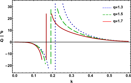
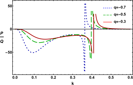
Figure 1: Plot of $P/Q$ vs $k$ for different values of positive $q$ when other plasma parameters are $\mu=2\times 10^{-6}$, $\nu=3\times 10^{5}$, $\alpha_{2}=0.5$, $\alpha_{3}=0.2$, and $\omega_{f}$.

Figure 2: Plot of $P/Q$ vs $k$ for different values of negative $q$ when other plasma parameters are $\mu=2\times 10^{-6}$, $\nu=3\times 10^{5}$, $\alpha_{2}=0.5$, $\alpha_{3}=0.2$, and $\omega_{f}$.

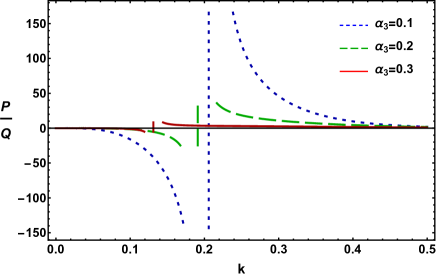
Figure 3: Plot of $P/Q$ vs $k$ for different values of positive $\alpha_{3}$ when other plasma parameters are $q=1.5$ $\mu=2\times 10^{-6}$, $\nu=3\times 10^{5}$, $\alpha_{2}=0.5$, and $\omega_{f}$.

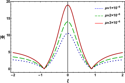
Figure 4: Plot of $Re(\Phi)$ vs $\xi$ for different values of $\mu$ when $k=0.3$, $\tau=0.0$, $q=1.5$, $\nu=3\times 10^{5}$, $\alpha_{2}=0.5$, $\alpha_{3}=0.2$, and $\omega_{f}$.

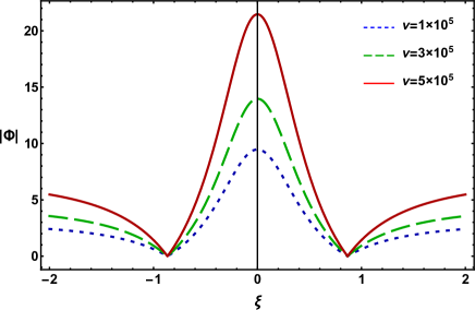
Figure 5: Plot of $Re(\Phi)$ vs $\xi$ for different values of $\nu$ when $k=0.3$, $\tau=0.0$, $q=1.5$, $\mu=2\times 10^{-6}$, $\alpha_{2}=0.5$, $\alpha_{3}=0.2$, and $\omega_{f}$.

Equation (39) describes that a large amount of wave energy, which causes due to the nonlinear characteristics of the medium, is localized into a comparatively small area in space.

5 Results and discussion

Now, we would like to numerically analyze the stability conditions of the DIAWs in presence of the non-extensive electrons. The mass and charge state of the plasma species even their number density are important factors in recognizing the stability conditions of the DIAWs in DPM [34, 35, 36, 37, 38, 39]. The mass of the dust grains is comparable to the mass of proton. In general picture of the DPM, dust grains are massive (millions to billions times heavier than the protons) and their sizes range from nanometres to millimetres. Dust grains may be metallic, conducting, or made of ice particulate. The size and shape of dust grains will be different, unless they are man-made. The dust grains are millions to billions times heavier than the protons, and typically, a dust grain acquires one thousand to several hundred thousand elementary charges [34, 35, 36, 37, 38, 39]. In this article, we consider three components dusty plasma model having inertial warm positive ions and negative dust grains, and interialess non-thermal non-extensive electrons. It may be noted here that in the DIAWs, if anyone consider the pressure term of the ions then it is important to be considered the moment of inertia of the ions along with the dust grains in presence of inertialess electrons. This means that the consideration of the pressure term of the ions highly contributes to the moment of inertia along with inertial dust grains to generate DIAWs in a DPM having inertialess electrons. In our present analysis, we have considered that $m_{d}=10^{6}m_{i}$, $Z_{d}=(10^{3}\thicksim 10^{5})Z_{i}$, and $T_{e}=10T_{i}$.

The detail picture of the non-extensive parameter (for both sub-extensive and super-extensive limits) in recognizing stable and unstable parametric regimes of the DIAWs can be observed in Figs. 2 and 2 for $\omega_{f}$ only, and it is obvious from this two figures that (a) both modulationally stable (i.e., $P/Q<0$) and unstable (i.e., $P/Q>0$) parametric regimes of the DIAWs can be obtained for sub-extensive (i.e., $q>1$) and super-extensive (i.e., $q<1$) limits of $q$; (b) the $k_{c}$ decreases with the increase in the value of $q$ within the limit of sub-extensive (i.e., $q>1$) but the $k_{c}$ increases with the increase in the value of $q$ within the limit of super-extensive (i.e., $q<1$); (c) so, the direction of the variation of $k_{c}$ totally depends on the sign of the $q$.

The influence of the charge state of positive ion, and the number density of the warm ions and electrons on the possible unstable and stable parametric regimes of DIAWs can be seen from Fig. 3 in which the variation of the $P/Q$ with $k$ for different values of $\alpha_{3}$ is shown when other plasma parameters are remain constant. It is clear from this figure that (a) when the parameter $\alpha_{3}$ is $0.1$, $0.2$, and $0.3$, then the corresponding $k_{c}$ is almost $0.21$, $0.20$, and $0.13$; (b) so, the stable window as well as the $k_{c}$ decreases with increasing $\alpha_{3}$; (c) the presence of excess number of non-extensive electrons dictates the DIAWs to be unstable as well allows to generate DIARWs for small wave number while the presence of excess number of warm ions dictates the DIAWs to be unstable as well allows to generate DIARWs for large wave number for a constant value of ion charge state (via $\alpha_{3}$).

The effects of inertial warm positive ion mass to inertial negatively charged massive dust grains mass (via $\mu$) on the formation of the DIARWs can be observed from Fig. 4, and it can be highlighted from this figure that (a) the increase in the value of $\mu$ does not only cause to change the nonlinearity of the plasma medium but also causes to increase the amplitude and width of the DIARWs; (b) physically, the nonlinearity of the plasma medium as well as the amplitude and width of the DIARWs increases (decreases) with the increase of positive ion mass (negative dust mass). Figure 5 demonstrates the influence of the ratio of the charge state of negative dust grains to the charge state of positive ion in recognizing the shape of the DIARWs in a nonlinear and dispersive plasma medium (via $\nu$). The amplitude and width of the DIARWs associated with modulationally unstable parametric regime decreases (due to the decrease of the nonlinearity of plasma medium) with positive ion charge state while increases (due to the increase of the nonlinearity of plasma medium) with negative dust grains charge state (via $\nu$).

6 Conclusion

In this paper, we have considered a dusty plasma model having inertial warm positive ions and negative dust grains, and inertialess non-extensive electrons to investigate the stability criteria, which determines by the sign of $P$ and $Q$ of NLSE, of the DIAWs according to the variation of plasma parameters, and have also observed the formation of DIARWs in the modulationally unstable parametric regime. The variation of the mass and charge state of the positive ion and negative dust grains has dictated a rigourous change in the configuration of DIARWs associated with DIAWs in the modulationally unstable parametric regime. The results from this brief study are to be applicable in explaining the formation of nonlinear electrostatic DIARWs in space (viz., Earth ionosphere [1], asteroid zones [2], magnetosphere [1], protostellar disks [2], molecular clouds [2], interstellar medium [1], cometary tails [2], and planetary rings [1], etc.) and laboratory plasmas.

References

• [1] S. K. El-Labany, et al., Phys. Plasmas 25, 013701 (2018).
• [2] P. Eslami, et al., IEEE Trans. Plasma Sci. 41, 3589 (2013).
• [3] P. Bandyopadhyay, et al., Phys. Rev. Lett. 101, 065006 (2008).
• [4] J. Heinrich, et al., Phys. Rev. Lett. 103, 115002 (2009).
• [5] S. I. Popel, et al., JETP Lett. 74, 362 (2001).
• [6] B. Sahu and M. Tribeche, Astrophys. Space Sci. 338, 259 (2012).
• [7] M. Ferdousi, et al., Eur. Phys. J. D 71, 102 (2017).
• [8] B. Sahu and M. Tribeche, Astrophys. Space Sci. 341, 573 (2012).
• [9] N. A. Chowdhury, et al., Chaos 27, 093105 (2017).
• [10] N. A. Chowdhury, et al., Phys. plasmas 24, 113701 (2017).
• [11] M. H. Rahman, et al., Chinese J. Phys. 56, 2061 (2018).
• [12] M. H. Rahman, et al., Phys. Plasmas 25, 102118 (2018).
• [13] N. A. Chowdhury, et al., Vacuum 147, 31 (2018).
• [14] C. Tsallis, J. Stat. Phys. 52, 479 (1988).
• [15] N. Akter, et al., J. Plasma Phys. 81, 905810518 (2015).
• [16] M. Bacha, et al., Phys. Rev. E 85, 056413 (2012).
• [17] A. Renyi, Acta Math. Acad. Sci. Hung. 6, 285 (1955).
• [18] N. A. Chowdhury, et al., Contrib. Plasma Phys. 58, 870 (2018).
• [19] N. Ahmed, et al., Chaos 28, 123107 (2018).
• [20] R. K. Shikha, et al., Eur. Phys. J. D 73, 177 (2019).
• [21] S. Jahan, et al., Commun. Theor. Phys. 71, 327 (2019).
• [22] M. Hassan, et al., Commun. Theor. Phys. 71, 1017 (2019).
• [23] N. A. Chowdhury, et al., Plasma Phys. Rep. 45, 459 (2019).
• [24] I. Kourakis and P.K. Shukla, Phys. Plasmas. 10, 3459 (2003).
• [25] W. M. Moslem, et al., Phys. Rev. E 84, 066402 (2011).
• [26] A. S. Bains, et al., Astrophys. Space Sci. 343, 621 (2013).
• [27] X. Jukui and L. He, Phys. Plasmas 10, (2003) 339.
• [28] H. R. Pakzad, et al., Astrophys. Space Sci. 353, 543 (2014).
• [29] C. Li, et al., Smart Mater. Struct. 20, 0152023 (2011).
• [30] C. Li, et al., Compos. Part B-Eng. 116, 153 (2017).
• [31] J. J. Liu, et al., J. Vib. Control 23, 3327 (2016).
• [32] J. J. Liu, et al., Appl. Math. Model 45, 65 (2017).
• [33] A. Ankiewicz, et al., Phys. Lett. A 373, 3997 (2009).
• [34] E. Saberiana, et al., Plasma Phys. Rep. 43, 83 (2017).
• [35] R. L. Merlino, J. Plasma Phys. 80, 773 (2014).
• [36] P. K. Shukla and B. Eliasson, Phys. Rev. E 86, 046402 (2012).
• [37] A. A. Mamun and P.K. Shukla, Phys. Scripta T98, 107 (2002).
• [38] M. Shalaby, et al., Phys. Plasmas 16, 123706 (2009).
• [39] P. K. Shukla and A.A. Mamun, Introduction to Dusty Plasma Physics (IOP, London, 2002).