Hierarchical Multiple-Instance Data
Classification with Costly Features

Abstract

We motivate our research with a real-world problem of classifying malicious web domains using a remote service that provides various information. Crucially, some of the information can be further analyzed into a certain depth and this process sequentially creates a tree of hierarchically structured multiple-instance data. Each request sent to the remote service is associated with a cost (e.g., time or another cost per request) and the objective is to maximize the accuracy, constrained with a budget. We present a generic framework able to work with a class of similar problems. Our method is based on Classification with Costly Features (CwCF), Hierarchical Multiple-Instance Learning (HMIL) and hierarchical decomposition of the action space. It works with samples described as partially-observed trees of features of various types (similar to a JSON/XML file), which allows to model data with complex structure. The process is modeled as a Markov Decision Process (MDP), where a state represents acquired features, and actions select yet unknown ones. The policy is trained with deep reinforcement learning and we demonstrate our method with both real-world and synthetic data.

I Introduction

Our work is motivated by a real-world problem of classifying whether a specific internet domain (e.g., google.com) is malicious. For this purpose, we use ThreatCrowd – a service providing rich security-oriented information about domains, such as known malware binaries communicating with the domain (identified by their hashes), WHOIS information, DNS resolutions, subdomains, associated email addresses, and, in some cases, a flag that the domain is known to be malicious (see an example of its interface in Figure 1). This information is stored in a graph structure, but only a part around a current pivot is visible to the user. However, the user can easily change the pivot and request more information about the connected objects. For example, after probing the main domain google.com, the user can focus on one of its multiple IP addresses to analyze its reverse DNS lookups, or which other domains are involved with a particular malware.

Figure 1: Threatcrowd’s interface. Various information is available for each node and the right side displays the information about the currently focused pivot. The left side shows a fraction of information graph around the pivot, unfolded to a limited depth.

ThreatCrowd provides an application programming interface (API) with a limited number of requests per unit of time. This makes the API a scarce resource which we have to account for. We also assume that the complete information graph is not available upfront, hence only the specifically requested information can be used. Some domains are unclassified, i.e., it is unknown whether they are malicious or not. We are interested in the following task:

Given a certain number of API requests, classify a specified domain using the available information, potentially changing the pivot to learn more information about the connected objects (malware hashes, emails, DNS information, etc.).

This is a classification task, restricted with a budget, and with information sequentially added over time (the complete information is not known in the beginning). The optimal solution requires sequential decision making, i.e., based on the information gathered so far, the algorithm decides the next step – either it acquires a new piece of information (until the budget is met), or it can end this process and return a classification decision. Moreover, the information gathered so far cannot be represented as a vector of a fixed size, mainly because the total number of all objects is variable and a-priori unknown (e.g., a single domain can be resolved to an arbitrary number of IP addresses, associated with multiple emails, etc.–).

While we started our motivation with ThreadCrowd, the described task is not exclusive to it and can be found in many other domains. For example, in targeted advertising in social networks, the goal is to show users an interesting advertisement. Each user can be described by a set of friends, posts or messages, where each object can contain rich features (and possibly nested sets, e.g., friends of friends). While analyzing a single user may be trivial, the cost of the used resources quickly becomes an important issue when scaling up. In medicine, the patients’ features consist of their medical history, tests results, or specialist examinations – all of which can vary in depth and breadth. Apart from the accuracy, there are other resources that we need to account for. In ThreatCrowd case it was the number of API requests. Frequently, an access to online APIs is monetized. In other domains, the valuable resources can be not only money but also time, patient’s discomfort, etc. Recently, we see that sustainability and ecology starts to play increasingly larger role and hence resources like electricity consumption or CO₂ production will gain importance. Therefore, we argue that algorithms taking these resources into account are needed.

I-A HMIL-CwCF Framework

In this manuscript, we present a generic framework to solve a class of classification problems similar to the described ThreatCrowd case. For demonstration purposes and to facilitate experimentation, we work with offline datasets, which represent the complete information graph and we simulate the sequential information retrieval, given a specific starting point. For example, to create the ThreatCrowd dataset, we used the API to extract all information about 1 171 domains within a depth of three requests (depth of 1 would be only the domains’ immediate features) and saved all this information in an offline dataset. In real deployments, we expect that an offline dataset with complete features can be acquired and used only for model training. During inference, only the requested features are available, and so a real interface has to be used, with all its limitations.

Our problem is an instance of Classification with Costly Features (CwCF) [1]. The task in this framework is, individually for each sample, to sequentially acquire features to maximize expected classification accuracy while minimizing the cost spent per sample. This cost can be designed to target a specific budget either on average or that the cost has to fit within the budget strictly for every sample. In this manuscript, we focus only the average budget case, but the modification to a strict budget is already studied in the prior work. We build our method upon the recent work of [2, 3] who used neural networks and deep reinforcement learning (RL). However, their framework is limited to samples described by feature vectors of a fixed size.

In this manuscript, we lift this limitation and develop a method that is capable of working with samples with hierarchical multiple-instance feature structure. That is, for a specific data (e.g., the ThreatCrowd data), a common schema exists that describes its structure and types (see Fig. 2b). Moreover, some parts of the hierarchy can be missing in a particular data instance and the data typically contains set objects – these objects contain arbitrary number of children (e.g., IP addresses for a particular domain). This is similar to JSON or XML data formats with a specified schema. To process this kind of data, we adopt Hierarchical Multiple-Instance Learning (HMIL) [4], which is a modular neural network architecture able to work with hierarchical data.

While HMIL is used to process the data at input, it is only one part of the solution. The CwCF algorithm is sequential in nature and uses deep reinforcement learning to find a policy to select and observe unknown features. However, the original CwCF algorithm assumes that there is a fixed number of features to select from and that the action space is static. In our case, these asssumptions are broken. First, the data contains set objects (possibly nested), which can contain different number of children per sample. Second, only a part of the complete data-point is visible at any moment (only the features requested by the algorithm up to the moment). Both of these facts mean that there are different number of actions available to the algorithm at any moment, since we map the visible features with unknown values to actions. Moreover, there is no a-priori known upper bound for the number of actions. To solve this problem, we take advantage of the hierarchical composition of the features and propose to decompose the policy analogically to their structure with hierarchical softmax [5]. We adopt this technique from from natural language processing and it was not used in the deep RL context before.

I-B Demonstration

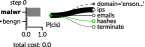
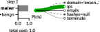
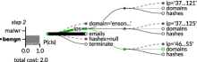
(b) dataset schema

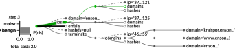
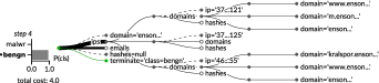
(a) steps of the sequential feature selection

Figure 2: (a) Classification of a potentially malicious domain (threatcrowd dataset). At each step, acquired features (full circles) and possible actions (empty circles) are shown. The method sequentially requests features (the policy is visualized as line thickness and the selection with a green line) – first, it retrieves (step 0) a list of known malware hashes communicating with the domain, (1) a list of associated IP addresses, (2, 3) and performs reverse IP lookups. The correct class is highlighted with a dot. Note that the number of actions differs at each step and the size of sets (IPs, hashes, and emails) differs between samples. The common schema for this dataset is shown in (b) with feature:type(cost) format. In this dataset, the costs represent API requests.

To better introduce the solved problem, we visualize how a trained algorithm works with a single sample from the threatcrowd dataset in Figure 2. A previously unseen sample is processed by the trained model and we visualize which features it requests and how the prediction changes. The algorithm starts with knowledge of the domain name only and can request various features, such as a list of associated IP addresses, emails, and hashes of known malware that communicates with the domain. Initially, only the domain name itself is known, without any additional details and the algorithm assigns the sample to the malware class (based on the distribution in the dataset). Next, the algorithm requests a list of malware hashes (there are not any) and a list of IP addresses (steps 0, 1). The prediction changes to benign, likely because there is no malware communicating with the domain and no malicious IP address is in the list. Still, the algorithm requests a reverse DNS lookup for two of the IP addresses, to confirm the prediction (steps 2, 3). Finally, the algorithm decides to finish with a correct classification benign. With four requests, the method was able to probe and classify an unknown domain. The balance between the number of requests and the expected accuracy is set with a budget during the training.

I-C Related Work

There is a number of existing algorithms working with costly features. Some employ decision trees [6, 7, 8, 9, 10, 11, 12], recurrent neural networks [13] or linear programming [14, 15]. [16] provide an analytical solution to optimally select features with a fixed order. There are multiple RL methods based on [1], e.g., by [2, 3, 17]. [18] uses RL with generative surrogate model that provides intermediary rewards by assessing the information gain of newly acquired features and other side information. Crucially, all of the mentioned techniques focus only on samples described by vectors of fixed dimensions (except for [17], who use a set of fixed-length vectors), and do not involve hierarchical features.

In Deep RL, the action space is usually formed with orthogonal dimensions and can be factorized in some way [19, 20, 21]. In our method, we factorize the complex action space with hierarchical softmax [5, 22], which was not used previously.

The problem is distantly related to graph classification algorithms (e.g., [23, 24, 25, 26]). These algorithms either aim to classify graph nodes or the graph itself as a whole. In our case, we assume that the hierarchical structure is a tree, constructed around a pivot of interest (e.g., a particular web domain). For this kind of data, the HMIL algorithm is better suited and less expensive than a general message-passing. Moreover, the graph classification algorithms do not involve sequential feature acquisition nor they account for costs of features.

II Background

This section describes the methods we build upon in this work. Our method is based on the Classification with Costly Features (CwCF) [3, 2] framework to set the objective and reformulate the problem as an MDP. However, structured data pose non-trivial challenges due to their variable input size and the variable number of actions. To create an embedding of the hierarchical input, we use Hierarchical Multiple-Instance Learning (HMIL) [4]. To select the performed actions, we use hierarchical softmax [5, 22]. To train our agent, we use Advantage Actor Critic (A2C) [27], a reinforcement learning algorithm from the policy gradient family.

II-A Classification with Costly Features

CwCF [2, 3] is a problem of maximizing accuracy, while minimizing the cost of features used in the process. Let $(y_{\theta},k_{\theta})$ be a model where $y_{\theta}$ returns the label and $k_{\theta}$ returns the features used. The objective is:

$$\min_{\theta}\mathop{\mathbb{E}}_{(x,y)\in\mathcal{D}}\big{[}\ell_{rl}(y_{\theta}(x),y)+\lambda c(k_{\theta}(x))\big{]}$$ (1)

Here, $(x,y)$ is a data point with its label, drawn from dataset $\mathcal{D}$, $\ell_{rl}$ is a classification loss, $c$ is the cost of the given features, and $\lambda$ is a trade-off factor between the accuracy and the cost. Minimizing this objective means minimizing the expected classification loss together with the $\lambda$-scaled per-sample cost. In the original framework, each data point $x\in\mathbf{R}^{n}$ is a vector of $n$ features, each of which has a defined cost. Note that one of the differences to this paper is that in our case, each data point can be composed of an arbitrary number of features of different sizes, structured in a tree.

Eq. (1) allows constructing an MDP with an equivalent solution to the original goal, and so standard reinforcement learning (RL) techniques can be used [1, 2]. In this MDP, an agent classifies one data point $(x,y)$ per episode. The state $s$ represents the currently observed features. At each step, the algorithm can either choose to reveal a single feature $k$ (and receive a reward of $-\lambda c(k)$) or to classify with a label $y_{\theta}(x)$, in which case the episode terminates, and the agent receives a reward of $-\ell_{rl}(y_{\theta}(x),y)$. We use a binary loss for $\ell_{rl}$ (0 in case of mismatch, -1 otherwise). Note that [2] define the classifier $y_{\theta}$ as an integral part of the MDP (i.e., special actions are mapped to different classes) and as such, it is directly optimized by the RL algorithm. To improve sample efficiency, we adopt a technique from [17] and use a separately trained classifier, that is simultaneously optimized along with the RL model. Modifications to the CwCF framework that allow an average or strict budget are available [1, 3].

II-B Hierarchical Multiple-Instance Learning

[28] introduce Multiple-Instance Learning (MIL); alternatively, [29] introduce Deep Sets, a neural network architecture to learn an embedding of an unordered set $\mathcal{B}$, composed of $m$ items $v_{\{1..m\}}\in\mathbf{R}^{n}$. The items are simultaneously processed into their embeddings $z_{i}=f_{\theta_{\mathcal{B}}}(v_{i})$, where $f_{\theta_{\mathcal{B}}}$ is a non-linear function with parameters $\theta_{\mathcal{B}}$, shared for the set $\mathcal{B}$. All embeddings are processed by an aggregation function $g$, commonly defined as a mean or max operator (in this work, we use the mean). The whole process creates an embedding $z_{\mathcal{B}}$ of the set and is differentiable. Hierarchical MIL [4] works with hierarchies of sets, corresponding to variable-sized trees. In this case, the nested sets (where different types of sets have different parameters $\theta_{\mathcal{B}}$) are recursively evaluated as in MIL, and their embeddings are used as feature values (see Figure 3a). The soundness of the hierarchical approach is theoretically studied by [30].

II-C Hierarchical Softmax

This technique is adapted from natural language processing [5, 22], where it was used to factorize a probability distribution $p(y\mid x)$ of a fixed number of tokens $y$ into a tree. Each node represents a decision point, itself being a proper probability distribution. Sampling from $p$ can be seen as a sequence of stochastic decisions at each node, starting from the root and continuing down the tree. If we label the probabilities encountered on the path from a root node to $y$ with $p_{1},\dots,p_{n}$, then $p(y\mid x)=\prod_{i=1}^{n}p_{i}$. In our work, we adapt this technique to work with an a priori unknown number of actions. In our case, the approach brings computational savings (only the probabilities on the selected path have to be computed) and semantical factorization of the probability space – i.e., the probability of selecting a feature down in the tree is dependent on probabilities of its parent objects.

II-D A2C Algorithm

To optimize our model, we use a synchronous implementation of Advantage Actor Critic algorithm (A2C) [27], an on-policy policy-gradient algorithm. A noteworthy fact is that the A2C method requires to compute the policy entropy, which is computationally expensive in our case. All feature probabilities would have to be computed, which also undermines one of the advantages of the hierarchical softmax. Inspired by [31], we estimate the gradient of the entropy $\nabla_{\theta}H_{\pi_{\theta}}(s)$ of a policy $\pi_{\theta}$ in a state $s$ as:

$$\nabla_{\theta}H_{\pi_{\theta}}(s)=-\mathop{\mathbb{E}}_{a\sim\pi_{\theta}(s)}\Big{[}\log\pi_{\theta}(a\mid s)\cdot\nabla_{\theta}\log\pi_{\theta}(a\mid s)\Big{]}$$ (2)

Provided we only know the probability of the actually selected action, we can use it to sample the expectation and use larger batches to reduce the variance. The detailed description of A2C and derivation of eq. (2) is in Supplementary Material A.

III Method

III-A Dataset Schema

Let us begin with a dataset schema, which describes the structure, features, their types and costs. E.g., in Figure 2b, the schema specifies that each sample contains a free feature domain with type string and sets of ips, emails and hashes. Objects in these sets have their own features (e.g., each ip address has a set of reversely translated domains). Note that in a particular instance, the set can hold an arbitrary number of items. The schema also defines a cost for each feature and set, which assumes that the cost of a particular feature across all samples is constant. While this assumption decreases the flexibility of the framework, we argue that it is reasonable for real-world data, where the cost of features can be usually precisely quantified upfront (e.g., the costs of medical examinations). When processing a sample, the cost needs to be paid to reveal the feature value or objects in a set (however, the features of these objects are not automatically visible).

To put it formally, let $\mathcal{D}=\{(x_{i},y_{i})\}_{i=1..n}$ be a dataset of samples $(x,y)$, where $x$ is a complete sample with all features and $y$ is a label. Let an object schema be a tree where the root children describe features with a tuple (name, type, cost), i.e., their name, data-type, and non-negative real-valued cost. Each node with a special type set is itself an object schema, and only these nodes can contain further children. A dataset schema $S$ is an object schema corresponding to the main object in the dataset (e.g., a user).

III-B Data Samples

The samples $x$ are an instantiation of the schema $S$. They are trees where nodes contain feature values of the specified types. Set nodes contain zero or more children, one for each existing object. These child nodes follow the structure specified in the schema for the set node.

When processing a sample, the agent does not see the complete feature tree of $x$, but only its fraction. Let $\bar{x}$ be an observation, a pruned version of full $x$. The nodes in $\bar{x}$ can be observed, meaning that we know their true value, or unobserved, in which case their value is unknown. For features, this means that their value from $x$ is included. For set nodes, being unobserved means that the node is truncated and without children. If it is observed, all children specified in $x$ are included. However, these children’s features follow the same principles and can also be observed or not. In other words, an observed set node can possibly contain only children without any further information (only their number is known), or with only some information about some of the children.

In each episode, the algorithm analyzes and classifies one sample $x$. The initial observation $\bar{x}_{0}$ contains only the root and its children, all unobserved. That is, the feature nodes do not contain their value, and set nodes are truncated. As an exception, the nodes with zero cost are automatically observed (for sets, this rule is applied recursively).

The algorithm starts with $\bar{x}_{0}$ and sequentially selects unobserved nodes to retrieve their values until it decides to terminate. We model the problem as an MDP, where a state is the current observation $\bar{x}$, and the set of actions contain one action for each unobserved node in $\bar{x}$, and a single terminal action $a_{t}$. Let $\bar{x}^{\prime}=o(x,\bar{x},a)$ be a new observation, created with the complete sample $x$, current observation $\bar{x}$ and an action $a$, that selects an unobserved node in $\bar{x}$. The function $o$ makes the selection $a$ in $\bar{x}$ observed (with the true value from $x$) and returns it as $\bar{x}^{\prime}$. The transition dynamics $t$ of the MDP is defined as:

$$t(\bar{x},a)=\begin{dcases*}\mathcal{T}&if $a=a_{t}$\\ o(x,\bar{x},a)&otherwise\end{dcases*}$$

where $\mathcal{T}$ is the terminal state. Let $\hat{y}$ be a classifier, $\ell_{rl}$ the binary loss function, $c(a)$ a cost of the feature selected by an action $a$ and $\lambda$ a cost-accuracy trade-off parameter. The reward function $r$ is:

$$r(\bar{x},a)=\begin{dcases*}-\ell_{rl}(\hat{y}(\bar{x}),y)&if $a=a_{t}$\\ -\lambda c(a)&otherwise\\ \end{dcases*}$$

The objective is to maximize the total expected reward over the distribution of samples in $\mathcal{D}$, which corresponds to the eq. (1). Moreover, we want a model that generalizes well to unseen data.

III-C Model

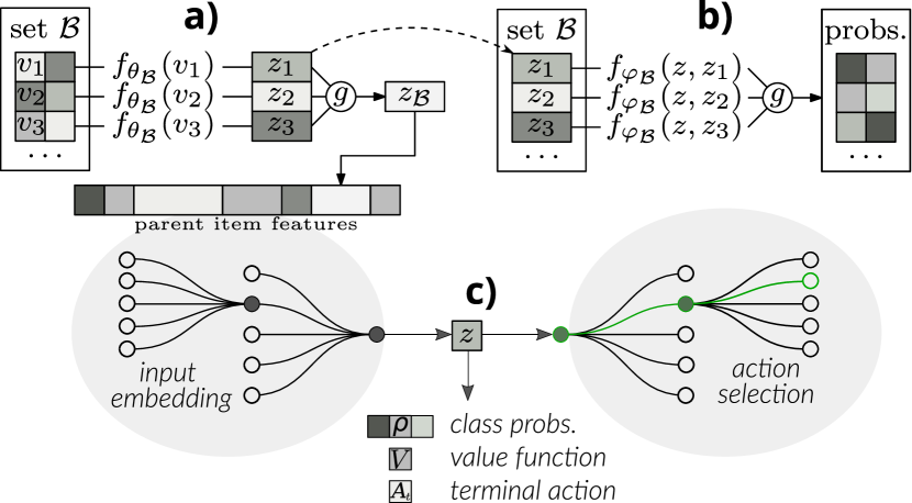
Figure 3: The input $\bar{x}$ is recursively processed to create embeddings $z_{i}$ for each object in the tree and the sample-level embedding $z$ (a, c left). The embedding $z$ is used to compute class probabilities $\rho$, value estimate $V$, and the terminal action potential $A_{t}$ (c middle). Then, an unobserved leaf node is chosen with a sequence of stochastic decisions (c right), with probabilities determined by the type of the set $\mathcal{B}$, and the previously computed embeddings (b).

The model is composed of several parts, displayed in Figure 3. First, the input $\bar{x}$ is processed with HMIL to create item-level and sample-level embeddings. Second, the sample-level embedding is used to return class probabilities, the value function estimate, and the terminal action value. Third, the probability distribution over actions is created with hierarchical softmax. Let us describe these parts in more detail.

III-C1 Input pre-processing

The features in $\bar{x}$ can be of different data types, and before the processing with a neural network, they have to be converted into real vectors. For strings, we observed good performance with character tri-gram histograms [32]. This hashing mechanism is simple, fast, and conserves similarities between strings. We used it for its simplicity and acknowledge that any other string processing mechanism is possible. One-hot encoding is used with categorical features. If the feature is unobserved, a zero vector of the appropriate size is used. To help the model differentiate between observed and unobserved features, each feature in $\bar{x}$ is augmented with a mask. It is a single real value, either $1$ if the feature is observed or $0$ if not. In sets, the mask is the fraction of the corresponding branch that is observed, computed recursively.

III-C2 Input embedding

(Figure 3ac) A neural network is created according to the schema $S$ and the HMIL algorithm. Let $\mathfrak{B}$ be a set of all sets present in the schema. For each $\mathcal{B}\in\mathfrak{B}$, parameters $\theta_{\mathcal{B}}$ are randomly initialized. The embedding functions $f_{\theta_{\mathcal{B}}}$ are implemented as one fully connected layer with LeakyReLU activation. Let $\Theta=\{\theta_{\mathcal{B}}:\mathcal{B}\in\mathfrak{B}\}$ denote all sets’ parameters and let $h_{\Theta}$ be the network’s HMIL part. The input $\bar{x}$ is recursively processed with $h_{\Theta}$ (see Background for more details), creating embeddings $f_{\theta_{\mathcal{B}}}(v)$ for each object $v$ in each set $\mathcal{B}$ and a sample-level embedding $z=h_{\Theta}(\bar{x})$.

III-C3 Classifier

(Figure 3c) The sample-level embedding $z$ encodes necessary information about the whole sample $\bar{x}$ that is enough to provide a class probability distribution $\rho(z)$ and the final decision $\hat{y}(\bar{x})=\mathop{\mathrm{argmax}}\rho(z)$. Since the classification is required only in terminal states, the unbiased loss respects their reach probabilities. Recalling that the observations $\bar{x}$ are states of the MDP, let $\mathcal{S}_{T}$ be a set of terminal states and $P_{\pi}(s)$ a reach probability of a state $s$ under a policy $\pi$, then the unbiased classification loss is:

$$L_{cls}=\mathop{\mathbb{E}}_{P_{\pi}(s)}[\ell_{cls}(\rho(s),y)]\;\mid\;s\in\mathcal{S}_{T}$$ (3)

To get an unbiased estimate, we can either train the classifier only in the encountered terminal states, or in every reached non-terminal state weighted by the terminal action probability. Since the latter provides a lower variance estimate, we use that. For $\ell_{cls}$, we use cross-entropy loss and we implement $\rho$ as a single linear layer followed by softmax.

III-C4 Value function and terminal action

The embedding $z$ is also used to compute the value function estimate $V(z)$ (required by the A2C algorithm) and pre-softmax value of the terminal action $A_{t}(z)$. Both functions are implemented as a single linear layer.

III-C5 Action selection

(Figure 3bc) Oppositely to the input embedding procedure, the action selection starts at the root of $\bar{x}$ and a series of stochastic decisions are made at each node, continuing down the tree. The root node is regarded as a set with a single object. For a specific observation $\bar{x}$ and set $\mathcal{B}\in\mathfrak{B}$, let $v_{1},...,v_{m}$ be the objects in the set, $z_{i}=f_{\theta_{\mathcal{B}}}(v_{i})$ their embeddings, and $z$ the sample-level embedding of $\bar{x}$, computed in the previous step. Also, let $K_{\mathcal{B}}$ be the number of immediate features at the level of $\mathcal{B}$ (as defined in the schema $S$) and $f_{\varphi_{\mathcal{B}}}(z,z_{i})\in\mathbf{R}^{K_{\mathcal{B}}}$ a function that transforms the global embedding $z$ and object-specific embedding $z_{i}$ into a vector (single scalar for each feature). The probability of selecting a feature $k$ in an object $v_{i}$ is then determined as $\mathop{\mathrm{softmax}}_{i,k}\big{(}f_{\varphi_{\mathcal{B}}}(z,z_{1}),...,f_{\varphi_{\mathcal{B}}}(z,z_{m})\big{)}$. The parameters $\varphi_{\mathcal{B}}$ are set-specific and different from $\theta_{\mathcal{B}}$, and the function $f_{\varphi_{\mathcal{B}}}$ is implemented as a single fully connected layer with no activation function. Observed features and fully expanded sets are excluded from the softmax. At the root level, the terminal action potential $A_{t}(z)$ is added to the softmax.

III-C6 Policy

Let $\pi_{\Omega}$ be the probability distribution over actions, where $\Omega=\{A_{t},\rho,V,\Theta,\varphi_{\mathcal{B}}:\mathcal{B}\in\mathfrak{B}\}$ is the set of all parameters in the model. The probability of selecting an action $a$ in the context of $\bar{x}$ is $\pi_{\Omega}(a\mid\bar{x})=\prod_{i=1}^{n}p_{i}$, where $p_{1},...,p_{n}$ are the probabilities in the selected path. We use the A2C algorithm that returns a policy gradient loss $L_{pg}$ at each step. The selection leading to an action makes the model interpretable because it reveals which objects and features contributed to the decision. It also saves computational resources because the whole distribution does not have to be computed, and it enables effective learning [19].

III-C7 Training

A batch of samples is processed parallelly, the policy gradient loss $L_{pg}$ and classification loss $L_{cls}$ are computed and the model is updated in a direction of $\nabla_{\Omega}(L_{pg}+\alpha_{cls}L_{cls})$, where $\alpha_{cls}$ is a training weight for the classifier. We use the A2C algorithm to demonstrate the method without the ambition to achieve the best performance possible – any recent RL improvement is likely to improve the performance. The exact implementation with hyperparameter settings is in Supplementary Material C.

III-C8 Pre-training classifier

The RL algorithm optimizes eq. (1), which assumes a trained classifier. However, the classifier is trained simultaneously by minimizing eq. (3). As the classifier output appears as a term in (1) and eq. (3) is based on terminal states probability $P_{\pi}$, this introduces nonstationarity in both problems. To mitigate the issue and speed up convergence, we pretrain the classifier $\rho$ with random states (pruned samples). We cannot target a specific budget, since it is unknown before the training (only a tradeoff parameter $\lambda$ is specified). Hence we cover the whole state space by generating partially constructed samples $\bar{x}$ ranging from almost-empty to complete. The exact details are in Supplementary Material C.

III-C9 Pre-training value function

Parallelly, we pretrain the value $V$ with the target $-\ell_{rl}(\hat{y}(\bar{x}),y)$, using the same random samples $\bar{x}$. This gives a lower bound for the optimal $V$ function since it assumes that the algorithm terminates and classifies at that point (either it is the best action, or not and then the value is higher).

IV Experiments

In this section, we describe several experiments that show the behavior of our algorithm and its ablations. We shared the complete code for all described algorithms and all datasets publicly at https://github.com/jaromiru/rcwcf.

IV-A Tested Algorithms

To our knowledge, there is not any other method dealing specifically with costly hierarchical data. For this reason, we created three ablations of the complete algorithm for comparison.

HMIL: Assuming that the complete information is available, we use directly the HMIL algorithm and train it in supervised manner. In theory, this approach should result in an upper bound estimate of the accuracy, but also with the highest cost. In practice, using all features at once makes the algorithm prone to overfitting, which we mitigated by using aggressive weight decay regularization [33].

Random: To see the influence of how the features are selected, we replace the policy part of the complete algorithm with a random sampling. This algorithm acquires features randomly until a specified budget is exceeded. All other parts of the algorithm are kept the same. Since this algorithm is uninformed, we expect it to underperform the complete algorithm and give a lower bound estimate for accuracy.

Flat-CwCF: With this ablation, we aim to demonstrate how the situation would change if the data was flattened – i.e., the root-level set features are considered as a single feature and the algorithm observes the complete sub-tree whenever such a feature is selected. This ablation behaves the same as the full algorithm on the root level, but it lacks the fine control over which features it requests deeper in the structure. Because of that, we expect the method to underperform the full algorithm with lower budgets, but to gradually reach the performance of HMIL.

Finally, we refer to the full method described in this paper as HMIL-CwCF. We searched for the optimal set of hyperparameters for each algorithm and dataset using validation data, and the complete table with all settings is in Supplementary Material C.

IV-B Experiment Setup

For each dataset, we ran HMIL with ten different seeds, Random with 30 different budgets linearly covering either $[0,10]$, $[0,20]$ or $[0,40]$ range (depending on the dataset) and Flat-CwCF and HMIL-CwCF with 30 different values of $\lambda$, logarithmically spaced in $[10^{-4},1.0]$ range. For each run, we selected the best epoch based on the validation data (for more details, see convergence graphs in Supplementary Material E). We plot the results of each run as a scatter plot with the average cost on the x-axis and accuracy on the y-axis. For better visualization, we interpolate the results using the LOWESS method [34] and show the mean performance (± one standard deviation) of HMIL across the whole x-axis.

IV-C Experiment A: Synthetic Dataset

In this experiment, we aim to demonstrate the behavior of our method and other tested algorithms on a purposefully crafted data. Note that this synthetic dataset is designed to demonstrate the differences between the algorithms and therefore our method (HMIL-CwCF) performs the best.

Figure 4: The schema of the synthetic dataset. The numbers in parentheses denote the costs of the corresponding features.

Let’s first explain the dataset’s structure (follow its schema in Figure 4). A sample contains two sets (set_a and set_b), each with ten items. Each item has two features – free feature item_key with a value 0 and item_value containing a random label. Randomly, a single item in one of the sets is chosen and its item_key is changed to 1 and the item_value to the correct sample label. Further, the feature which_set contains the information about which set contains the indicative item. The idea is that the algorithm is able to learn a correct label by retrieving the which_set feature, opening the correct set, and retrieving the value for item with item_key=1. Uniquely for this dataset, we test the algorithms directly on the training data.

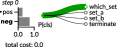
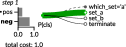
Figure 5: Results in the synthetic dataset. Left: The process of feature selection. In this example, the algorithm optimally requests the which_set feature, opens set_a and learns the label in the indicative item. Right: Performance of all algorithms across different budget settings (x-axis). We show our method (HMIL-CwCF), its ablation with a random policy (Random), ablation with flattened data (Flat-CwCF) and the HMIL algorithm trained with complete information. We train 30 instances per each algorithm (HMIL-CwCF, Random and Flat-CwCF), each targetting a different budget and plot each result with a point, along with a smoothed interpolation.

The Figure 5-right shows the performance of the tested algorithms in this dataset. For more details about how these experiments were executed, see Experiment Setup. HMIL (the ablation with complete data) reaches 100% accuracy with the total cost of 31 (cost of all features). The Flat-HMIL is able to reduce the cost by acquiring only the correct set, but has to retrieve it completely. Hence, it also reaches 100% accuracy, but with the cost of 16 (1 for which_set feature, 5 for one of the sets, and 10 for all values inside). Contrarily, the complete HMIL-CwCF method reaches 100% accuracy with only the cost of 7, since it can retrieve only the single indicative value from the correct set. Moreover, it is able to reduce the cost even further by sacrificing accuracy, as seen in the clustering around the cost of 6 and 0.75 accuracy, something that Flat-HMIL cannot do. This is one of the strengths of the proposed method – because it has greater control over which features it acquires, the user can choose to sacrifice the accuracy for a lower cost. Lastly, the Random method selects the features randomly, and hence its accuracy is well below HMIL-CwCF for corresponding budgets. The accuracy is influenced by the probability of getting the indicative item, which raises with the allocated budget and would reach 100% with the cost of 31 (we run the method with budgets from $[0,20]$).

We selected one of the models that was trained to reach 100% accuracy and examined how it behaves (see Figure 5-left). We see that it indeed learned to acquire which_set feature, open the corresponding set_a or set_b and select the item_value of the item with item_key=1 to learn the right label.

This experiment validates the correct behavior of our method and demonstrates the need for all its parts. Compared to HMIL and Flat-CwCF, the complete method reaches comparable accuracy with lower cost. Moreover, compared to Flat-CwCF, it has better control over which features it requests, achieving better accuracy even in the low-cost region. Finally, the order in which the features are acquired matter, as shown in comparison with Random.

IV-D Experiment B: ThreatCrowd

Let us focus on the real-world case which motivated this work. We sourced an offline dataset directly from the ThreatCrowd service through their API (with their permission). Programmatically, we gathered information about 1 171 domains within a depth of three API requests (including one request for the domain itself) around the original domain and split them to traning, validation and test sets. Each domain contains its URL as a free feature and a list of associated IP addresses, emails, and malware hashes. These objects can be further reverse-looked up for other domains. The ThreatCrowd interface, dataset schema, and the analysis of the algorithm’s behavior are shown in Introduction in Figures 1 and 2.

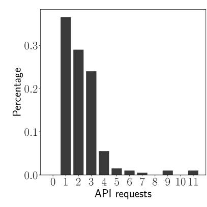
(a) results	(b) histogram of used API requests

Figure 6: (a) Results in threatcrowd dataset. The shaded area shows ± one standard deviation around the mean performance of HMIL (10 runs), across the whole x-axis for comparison. (b) Histogram of used API requests for a trained model that uses two requests on average.

The results of the experiment are shown in Figure 6a. The HMIL reaches the mean accuracy of $0.83$ with a cost of $15$. The other algorithms reach the same accuracy with lower mean cost, Flat-CwCF with $11$, Random with $5$ and HMIL-CwCF with only $2$ (results are rounded). That means that our method needs only two API requests on average to reach the same accuracy as HMIL (which uses complete information), resulting in $7.5\times$ savings. To give a better insight about what these two requests on average mean, we analyzed a single trained model and plot a histogram of API requests accross the whole test set in Figure 6b. With a single request, the algorithm can learn, for example, a list of all IP addresses (without further details) or a list of associated malware hashes. The histogram shows that in about 36% of samples, a single request is enough for classification, 29% requires two, 23% three and 12% four requests or more.

The results indicate that only a fraction of the available information is required to correctly classify a domain. The Flat-CwCF algorithm always acquires a complete sub-tree for a specific feature (e.g., a complete list of IP addresses with their reverse lookups, up to the defined depth), resulting in unnecessarily high cost. The results of Random show that only fraction of this information is required, even if randomly sampled. Finally, the complete method HMIL-CwCF shows that informed feature selection outperforms random sampling.

To conclude, this experiment verifies that all parts of the algorithm are required in a real-world scenario. To utilize a trained model in practice, one only requires an interface connecting the model’s input and decisions with the ThreatCrowd API.

IV-E Experiment C: Other Datasets

To further evaluate our method, how it scales with small and large datasets and how it performs in binary and multi-class settings, we sourced five more datasets from various domains. Because our method targets a novel problem, we did not find datasets in appropriate format – i.e., datasets with hierarchical structure and cost information. Therefore we transformed existing public relational datasets into hierarchical forms by fixing a pivot object (different for each sample) and expanding its neighborhood into a defined depth. We also manually added costs to the features in a non-uniform way, respecting that in reality, some features are more costly than others (e.g., getting a patient’s age is easier than doing a blood test). In practice, the costs would be assigned to the real value of the required resources. The depth of the datasets was chosen so that they completely fit into the memory.

IV-E1 Dataset descriptions

We provide brief descriptions of the used datasets below. The statistics are summarized in Table I. For reproducibility, we published the processed versions, along with a library to load them with the code. More details on how we obtained and processed the datasets, their splits, structure and feature costs are in Supplementary Material B.

TABLE I: Statistics of the used datasets. The features column shows the number of features (tree leaves) across all completely observed samples in the corresponding dataset.

dataset	samples	classes	class distribution	features	depth
	(all splits)			(min/mean/max)
synthetic	12	2	0.5 / 0.5	41 / 41.0 / 41	2
threatcrowd	1 171	2	0.27 / 0.73	4 / 118.7 / 1062	3
hepagenesis	500	2	0.41 / 0.59	158 / 305.2 / 47	2
mutagenesis	188	2	0.34 / 0.66	1 / 10.8 / 65	3
ingredients	39 774	20	0.01$\sim$0.20	15 / 30.8 / 51	2
sap	35 602	2	0.5 / 0.5	7 / 44.1 / 18537	2
stats	8 318	3	0.49 / 0.38 / 0.12	1 / 679.6 / 3604	3

Hepatitis: A relatively small medical dataset containing patients infected with hepatitis, types B or C. Each patient has various features (e.g., sex, age, etc.) and three sets of indications. The task is to determine the type of disease.

Mutagenesis: Extremely small dataset (188 samples) consisting of molecules that are tested on a particular bacteria for mutagenicity. The molecules themselves have several features and consist of atoms with features and bonds.

Ingredients: Large dataset containing recipes that have a single list of ingredients. The task is to determine the type of cuisine of the recipe. The main challenge is to optimally decide when to stop analyzing the ingredients.

SAP: In this large artificial dataset, the task is to determine whether a particular customer will buy a new product based on a list of past sales. A customer is defined by various features and the list of sales.

Stats: An anonymized content dump from a real website Stats StackExchange. We extracted a list of users to become samples and set an artificial goal of predicting their age category. Each user has several features, a list of posts, and a list of achievements. The posts also contain their own features and a list of tags and comments.

IV-E2 Results

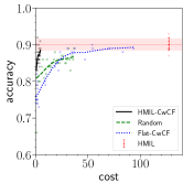
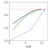
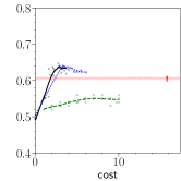
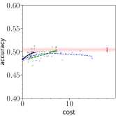
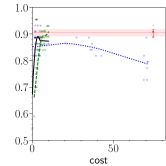
(a) hepatitis	(b) ingredients	(c) sap	(d) stats	(e) mutagenesis

Figure 7: The performance of the algorithms in five datasets, shown in the cost vs. accuracy plane. We show our method (HMIL-CwCF), its ablation with a random policy (Random), ablation with flattened data (Flat-CwCF) and the HMIL algorithm trained with complete information. We train 30 instances per each algorithm (HMIL-CwCF, Random and Flat-CwCF), each targetting a different budget and plot each result with a point, along with a smoothed interpolation. The HMIL is run 10 times and we plot the mean ± one standard deviation (the bar visualizes the metrics across the whole range of budgets for comparison).

The results are shown in Figure 7. Since the HMIL algorithm can access all features at once, it creates the top baseline. The variance of the results is high in hepatitis and mutagenesis datasets (Fig. 7ae), which is given by their small size, and this fact translates into the other methods as well.

The results in sap (Fig. 7c) are noteworthy. Here, the top accuracy of HMIL is exceeded by HMIL-CwCF and Flat-CwCF. We investigated what is happening and concluded that HMIL overfits the training data, despite aggressive regularization. In this case, there is a large gap between the training and validation accuracy, which narrowed with increased weight decay, but the validation accuracy was worse. Surprisingly, HMIL-CwCF and Flat-CwCF do not suffer from this issue, with less features. We hypothesize that the sap dataset contains some features that are very informative on the training set, but do not translate well to the test set. The well-performing methods are able to circumvent the issue by selecting fewer features, which results in less overfitting.

Generally, the HMIL-CwCF performs the best on all datasets, i.e., it reaches the same accuracy with lower cost. Compared to HMIL, the cost is reduced about $26\times$ in hepatitis, $1.2\times$ in ingredients, $8\times$ in sap, $6\times$ in stats and $15\times$ in mutagenesis, which are significant savings.

Flat-CwCF generally exhibits low performance in the low-cost region, due to its limited control over which features it gathers. The effect is exemplary in ingredients (Fig. 7b), where it is almost all-or-nothing – the results are clustered either in the no-feature range or in (almost) all-features range. In mutagenesis, Flat-CwCF largely underperforms HMIL in the high-cost region, although we extensively tried to optimize its parameters. We attribute the issue to the fact that mutageneis is extremely small (188 samples) and there is a significant distribution shift between the data splits. HMIL may be resilient to this effect, while HMIL-CwCF and Random do not display the behavior because they operate only in the low-cost region.

Lastly, let us point out the result of HMIL-CwCF compared to Random in ingredients (Fig. 7b). This dataset contains a single set of ingredients, which are objects with single feature. Hence, the dataset allows only random sampling, which intuitively makes HMIL-CwCF and Random the same method. However, while Random always uses the whole budget, HMIL-CwCF can select a different number of features for each sample. Hence it can classify early, if it randomly samples informative features, reaching a higher accuracy with the same average cost as Random.

IV-F Remarks

IV-F1 Explainability

Unlike the standard classification algorithms (e.g., HMIL), the sequential nature of HMIL-CwCF enables easier analysis of its behavior. Figures 2 and 5 present two examples of the feature acquisition process and give insight into the agent’s decisions. The weights the model assigns to different features in different samples and steps can be used to assess the agent’s rationality or learn more about the dataset. We present more visualizations in Supplementary Material D.

IV-F2 Computational requirements

We measured the training times using single core of Intel Xeon Gold 6146 3.2GHz and 4GB of memory (no GPU). On the synthetic dataset, the methods took 1 hr. / 1 min. / 30 min. / 1 hr. for HMIL-CwCF / HMIL / Random / Flat-CwCF respectively. The training times in other datasets were comparable, hence we present their average: 19 hrs. / 1 hr. / 14 hrs. / 9 hrs. for HMIL-CwCF / HMIL / Random / Flat-CwCF respectively. Note that the training times are for a single run (i.e., a single point in the Fig. 7), but the runs are independent and are easily parallelized. After training, the inference time is negligible for all methods.

Note that while the training time of HMIL-CwCF is much longer than in the case of HMIL, it is easily compensated by the fact that our method has the potential to save large amount of resources if correctly deployed. Moreover, computational power raises exponentially every year (resulting in faster training), while resources like CO₂ production, patients’ discomfort or response time of antivirus software only gains importance.

V Discussion

Comparison with Graph Neural Networks (GNNs).

Instead of HMIL, we could use a GNN to perform the input embedding. However, note that the datapoints we work with are constructed around a central pivot and all other information is hierarchically structured around it. Hence it makes sense to model the data as trees, not as general graphs, and use a method tailored to work with trees. In our case, generic message passing is not necessary and a single pass from leaves to the root of the tree is sufficient to correctly embed all information. [35] provides a deeper discussion about using HMIL and GNNs in sample-centric applications.

In some special cases, there could be a shared object within the hierarchy, located in multiple places (e.g., the same IP address accessible by multiple paths). In our method, we still handle the sample as a tree and these shared objects as if they were different. We argue that due to rather rare occurrences and the limited depth of our datasets, these cases do not influence the results and can be neglected.

Is the depth of the tested datasets sufficient?

We argue that most of the relevant information is within a near neighborhood of the central object of interest. Increasing the depth also results in exponential increase of the available feature space, potentially slowing training and involving increased space requirements. The experiments also showed that there are substantial differences between the tested methods, hence we conclude that the tested depth is sufficient.

How to obtain credible cost assignment?

For real-world usage, we assume that the costs can be measured upfront (e.g., time required, electricity consumed) or at least approximated, and that this cost is fixed. Datasets with this information are scarce and usually private. In Experiment C, we selected only datasets that can be made public and these come without the cost information. Hence we assigned them based on our opinion.

VI Conclusion

Motivated by a real-world problem of malicious domain classification, where the data is composed of hierarchically structured features with costs, we combine three distinct methods (Classification with Costly Features, Hierarchical Multiple-Instance Learning and Hierarchical Softmax) into a Deep RL-based algorithm that accepts incomplete tree-structured input and sequentially selects more features from the hierarchy to maximize accuracy and minimize the cost. Crucially, the method differs from previous approaches (which targeted fixed-length vector samples) with its ability to directly work with the tree-structured input. We demonstrate the algorithm with ThreatCrowd, a real-world domain classification service, and perform experiments in six more publicly available datasets from various domains. We compare its performance to three different ablations and show that it achieves comparable accuracy with better cost savings. Moreover, we visualize the algorithm’s decision on selected samples and demonstrate its explainability.

Supplementary Material

Hierarchical Multiple-Instance Data Classification with Costly Features

Part A A2C Algorithm

Advantage Actor Critic algorithm (A2C), a synchronous version of A3C [27], is an on-policy policy-gradient algorithm. It iteratively optimizes a policy $\pi_{\theta}$ and a value estimate $V_{\theta}$ with model parameters $\theta$ to achieve the best cumulative reward in a Markov Decision Process (MDP) $(\mathcal{S},\mathcal{A},r,t)$, where $\mathcal{S},\mathcal{A}$ represent the state and action spaces, and $r$, $t$ are reward and transition functions. Let’s define a state-action value function $Q(s,a)=\mathop{\mathbb{E}}_{s^{\prime}\sim t(s,a)}[r(s,a,s^{\prime})+\gamma V_{\theta}(s^{\prime})]$ and an advantage function $A(s,a)=Q(s,a)-V_{\theta}(s)$. Then, the policy gradient $\nabla_{\theta}J$ and the value function loss $L_{V}$ are:

$$\nabla_{\theta}J=\mathop{\mathbb{E}}_{s,a\sim\pi_{\theta},t}\Big{[}A(s,a)\cdot\nabla_{\theta}\log\pi_{\theta}(a\mid s)\Big{]}$$

$$L_{V}=\mathop{\mathbb{E}}_{s,a,s^{\prime}\sim\pi_{\theta},t}\Big{[}q(s,a,s^{\prime})-V_{\theta}(s)\Big{]}^{2}$$

$$q(s,a,s^{\prime})=\text{clip}(r(s,a,s^{\prime})+\gamma V_{\theta^{\prime}}(s^{\prime}),-\infty,1.)$$

where in $\theta^{\prime}$ is a fixed copy of parameters $\theta$. To stabilize training, we clip the target $q$ into $(-\infty,1.0)$, using the fact that the maximal $Q$ value is $1.0$ (the reward for correct prediction is $1.0$ and every other step has negative reward).

To prevent premature convergence, a regularization term $L_{H}$ in the form of the average policy entropy is used:

$$L_{H}=\mathop{\mathbb{E}}_{s\sim\pi_{\theta},t}\Big{[}H_{\pi_{\theta}}(s)\Big{]}\;;\;H_{\pi}(s)=-\mathop{\mathbb{E}}_{a\sim\pi(s)}\Big{[}\log\pi(a\mid s)\Big{]}$$

The computation of the policy entropy requires knowledge of all action probabilities, which is very expensive to compute in our case. Hence, we propose to estimate the gradient of the entropy directly as [31]:

$$\nabla_{\theta}H_{\pi_{\theta}}(s)=-\mathop{\mathbb{E}}_{a\sim\pi_{\theta}(s)}\Big{[}\log\pi_{\theta}(a\mid s)\cdot\nabla_{\theta}\log\pi_{\theta}(a\mid s)\Big{]}$$ (2 revisited)

and use only the performed action to sample the expectation with zero bias; the variance can be lowered with larger batches.

The total loss is computed as $L_{pg}=-J+\alpha_{v}L_{V}-\alpha_{h}L_{H}$, with $\alpha_{v},\alpha_{h}$ learning coefficients. The algorithm iteratively gathers sample runs according to a current policy $\pi_{\theta}$, and the traces are used as samples for the above expectations. Then, an arbitrary gradient descent method is used with the gradient $\nabla_{\theta}L_{pg}$. We run multiple environments in parallel to get a better gradient estimate. Note that while [27] used asynchronous gradient updates, we make the updates synchronously.

For reference, we include a derivation of eq. (2) below. For readability, we omit $\theta$ in $\nabla_{\theta}$ and $\pi_{\theta}$:

Derivation of eq. (2).

$$\nabla H_{\pi}(s) =-\nabla\sum_{a}\pi(a\mid s)\cdot\log\pi(a\mid s)$$

$$=-\sum_{a}\nabla\pi(a\mid s)\cdot\log\pi(a\mid s)-\sum_{a}\pi(a\mid s)\cdot\nabla\log\pi(a\mid s)$$

Using the fact $x\cdot\nabla\log x=\nabla x$, we show that the second term is zero:

$$\sum_{a}\pi(a\mid s)\cdot\nabla\log\pi(a\mid s)=\sum_{a}\nabla\pi(a\mid s)=\nabla\sum_{a}\pi(a\mid s)=\nabla 1=0$$

Let’s continue with the remaining term and use the fact $\nabla x=x\cdot\nabla\log x$ again:

$$\nabla H_{\pi}(s) =-\sum_{a}\nabla\pi(a\mid s)\cdot\log\pi(a\mid s)$$

$$=-\sum_{a}\pi(a\mid s)\cdot\nabla\log\pi(a\mid s)\cdot\log\pi(a\mid s)$$

$$=-\mathop{\mathbb{E}}_{a\sim\pi(s)}\Big{[}\nabla\log\pi(a\mid s)\cdot\log\pi(a\mid s)\Big{]}$$

∎

Part B Dataset Details

Hepatitis, mutagenesis, SAP and stats datasets were retrieved from [36] and processed into trees by fixing the root and unfolding the graph into a defined depth, if required. The threatcrowd dataset was sourced from the ThreatCrowd service, with permission to share. Ingredients dataset was retrieved from Kaggle.

Float values in all datasets are normalized. Strings were processed with the tri-gram histogram method [32], with modulo 13 index hashing. The datasets were split into training, validation, and testing sets as shown in Table II. The dataset schemas, including the feature costs, are in Figure 8.

TABLE II: Dataset statistics.

dataset	total samples	#train	#validation	#test	class distribution
synthetic	12	4	4	4	0.5 / 0.5
threatcrowd	1 171	771	200	200	0.27 / 0.73
hepatitis	500	300	100	100	0.41 / 0.59
mutagenesis	188	100	44	44	0.34 / 0.66
ingredients	39 774	29774	5000	5000	0.01$\sim$0.20
sap	35 602	15602	10000	10000	0.5 / 0.5
stats	8 318	4318	2000	2000	0.49 / 0.38 / 0.12

.1 domain. .2 domain:string(0). .2 ips[]:set(1.0). .3 ip:ip_address(0). .3 domains[]:set(1.0). .4 domain:string(0). .2 emails[]:set(1.0). .3 email:string(0). .3 domains[]:set(1.0). .4 domain:string(0). .2 hashes[]:set(1.0). .3 scans[]:set(1.0). .4 scan:string(0). .3 domains[]:set(1.0). .4 domain:string(0). .3 ips[]:set(1.0). .4 ip:ip_address(0). (a) threatcrowd

.1 user. .2 views:real(0.5). .2 reputation:real(0.5). .2 profile_img:real(0.5). .2 up_votes:real(0.5). .2 down_votes:real(0.5). .2 website:real(0.5). .2 about_me:string(1.0). .2 badges[]:set(1.0). .3 badge:string(0.1). .2 posts[]:set(1.0). .3 title:string(0.2). .3 body:string(0.5). .3 score:real(0.1). .3 views:real(0.1). .3 answers:real(0.1). .3 favorites:real(0.1). .3 tags[]:set(0.5). .4 tag:string(0.1). .3 comments[]:set(0.5). .4 score:real(0.1). .4 text:string(0.2). (b) stats

.1 patient. .2 sex:binary(0). .2 age:category(0). .2 bio[]:set(0.0). .3 fibros:category(1.0). .3 activity:category(1.0). .2 indis[]:set(0.0). .3 got:category(1.0). .3 gpt:category(1.0). .3 alb:binary(1.0). .3 tbil:binary(1.0). .3 dbil:binary(1.0). .3 che:category(1.0). .3 ttt:category(1.0). .3 ztt:category(1.0). .3 tcho:category(1.0). .3 tp:category(1.0). .2 inf[]:set(0.0). .3 dur:category(1.0). (c) hepatitis

.1 recipe. .2 f0[]:set(0). .3 igd:string(1.0). (d) ingredients

.1 object. .2 which_set:category(1.0). .2 set_a[]:set(5.0). .3 item_key:category(0.0). .3 item_value:category(1.0). .2 set_b[]:set(5.0). .3 item_key:category(0.0). .3 item_value:category(1.0). (e) synthetic

.1 customer. .2 sex:real(1.0). .2 marital_status:category(1.0). .2 educationnum:category(1.0). .2 occupation:category(1.0). .2 data1:real(1.0). .2 data2:real(1.0). .2 data3:real(1.0). .2 nom1:category(1.0). .2 nom2:category(1.0). .2 nom3:category(1.0). .2 age:real(1.0). .2 geo_inhabitants:real(1.0). .2 geo_income:real(1.0). .2 sales[]:set(1.0). .3 date:real(0.1). .3 amount:real(0.1). (f) sap

.1 molecule. .2 ind1:binary(1.0). .2 inda:binary(1.0). .2 logp:real(1.0). .2 lumo:real(1.0). .2 atoms[]:set(0.0). .3 element:category(0.5). .3 atom_type:category(0.5). .3 charge:real(0.5). .3 bonds[]:set(0.5). .4 bond_type:category(0.1). .4 element:category(0.1). .4 atom_type:category(0.1). .4 charge:real(0.1). (g) mutagenesis

Figure 8: Datasets schemas used in this work. The trees show the feature names, their types, and their cost in parentheses. Features with a set type contain an arbitrary number of same-typed items.

Part C Implementation and Hyperparameters

The hyperparameters for each method are summarized in Table III. For each model, we searched for an optimal set of hyperparameters – batch size in $\{128,256\}$, learning rate in $[3\times 10^{-4},1\times 10^{-3},3\times 10^{-3},1\times 10^{-2}]$, embedding size in $\{64,128\}$, weight decay in range $[1\times 10^{-4},3.0]$ and $\alpha_{h}$ in $\{0.0025,0.025,0.5,0.1\}$. We report that properly tuned weight decay and $\alpha_{h}$ is crucial for good performance.

The model’s architecture and parameters are initialized according to the provided dataset schema, and parameters $\theta_{\mathcal{B}},\varphi_{\mathcal{B}}$ are created for each set $\mathcal{B}$. LeakyReLu is used as the activation function. The aggregation function $g$ is mean with layer normalization [37]. The policy entropy controlling weight ($\alpha_{h}$) decays with $\frac{1}{T}$ schedule every 10 epochs. We use AdamW optimizer [33] with weight decay regularization. The learning rate of the main training in annealed exponentially by a factor of $0.5$ every 10 epochs. The gradients are clipped to a norm of $1.0$. For each dataset, we select the best performing iteration based on its validation reward.

C-A Pretraining

Before the main training, the classifier $\rho$ and the value output $V$ are initialized by pretraining. The classifier is pretrained with randomly generated partial samples from the dataset, with cross-entropy loss, $\alpha_{\rho}$ weight and the initial learning rate. To cover the whole state space, the partial samples are constructed as follows: A probability $p\sim\mathcal{U}_{[0,1]}$ is chosen and, starting from the root of the sample, features are included with probability $p$. All items in the sets are recursively processed in the same manner and the same probability $p$. The pretraining proceeds for a whole epoch (with the same batch size as in the main training) and subsequently the validation loss is estimated using the complete samples every $\frac{1}{10}$ of an epoch. Early stopping is used to terminate the pretraining. Simultaneously, with the same generated samples, the $V$ output is pretrained using L2 loss and $-\ell_{rl}(\hat{y}(\bar{x}),y)$ target, using the current $\rho$: $\hat{y}(x)=\mathop{\mathrm{argmax}}\rho(\bar{x})$, with $\alpha_{v}$ weight.

TABLE III: Hyper-parameters. If a hyper-parameter is not specified, it is the same as in HMIL-CWCF.

parameter	shared	synthetic	hepatitis	mutagenesis	ingredients	sap	stats	threatcrowd
HMIL-CwCF
steps in epoch	1000	100
train time (epochs)	200				300
batch size	256
embedding size ($f_{\theta_{\mathcal{B}}}$)	128
learning rate (initial)	1.0e-3
learning rate (final)	1.0e-3 / 30
learning rate decay factor	0.5 (every 10 epochs)
gradient max norm	1.0
$\gamma$ - discount factor	0.99
$\alpha_{\rho}$ - class. training weight	1.0
$\alpha_{v}$	0.5
$\alpha_{h}$ (initial)		0.025	0.1	0.025	0.05	0.1	0.05	0.05
$\alpha_{h}$ (final)		0.00025	0.005	0.00025	0.0025	0.005	0.0025	0.0025
weight decay		1e-4	1e-4	1e-4	0.3	1e-4	1e-4	3.0
HMIL
steps in epoch	100
train time (epochs)	50				200
learning rate (initial)	3.0e-3
learning rate (final)	3.0e-3 / 30
weight decay		1e-4	1.0	1.0	1.0	0.1	3.0	3.0
Flat-CwCF
steps in epoch	1000	100
train time (epochs)	200
$\alpha_{h}$ (initial)	0.05
$\alpha_{h}$ (final)	0.0025
weight decay		1e-4	1.0	1.0	1.0	0.1	1.0	3.0
Random
steps in epoch	1000	100
train time (epochs)		20	20	20	100	40	40	20
learning rate (initial)	3.0e-3
learning rate (final)	3.0e-3 / 30
weight decay		1e-4	1e-4	1.0	1.0	0.1	3.0	3.0

Part D Sample Runs

Below we show one selected sample from each dataset as processed by the proposed algorithm (we omit hepatitis and mutagenesis, as the samples are too large to visualize). Read left-to-right, top-to-down. At each step, the current observation is shown, the line thickness visualizes the action probabilities and the green line marks the selected action. On the left, there is a visualization of the current state value and class probabilities. The correct class is visualized with a dot, and the current prediction is in bold. All displayed models were trained with $\lambda=0.00108264$.

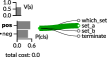
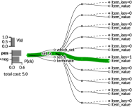
0:  1:  2: 

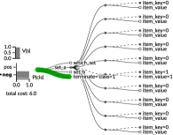
Figure 9: Sample from dataset synthetic

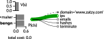
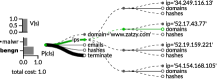
0:  1:  2: 

Figure 10: Sample from dataset threatcrowd

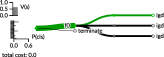
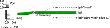
0:  1: 
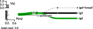
2:  3: 

Figure 11: Sample from dataset ingredients

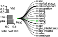
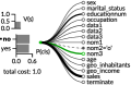
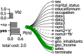
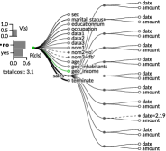
0:  1:  2:  3: 
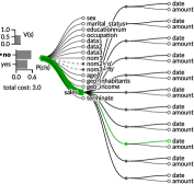
4:  5: 

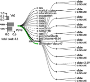
Figure 12: Sample from dataset sap

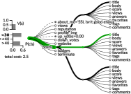
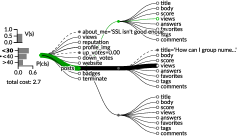
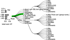
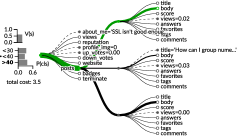
0:  1:  2: 
3:  4:  5: 
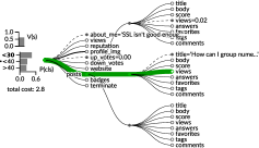
6:  7: 
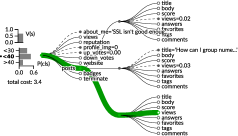
8:  9: 

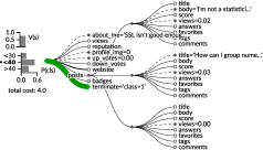
Figure 13: Sample from dataset stats

Part E Convergence Graphs

For each dataset, we present four different runs with different $\lambda$ in the following figures. Each subfigure, corresponding to a single run, is divided into three diagrams, showing the progression of average reward, cost and accuracy during the training. The reader can use the plots to examine behavior of the algorithm (mainly the importance of cost vs. accuracy) when run with different parameters $\lambda$. Evaluation on training, validation and testing sets is shown. The best iteration (based on the validation reward) is displayed by the dashed vertical line.

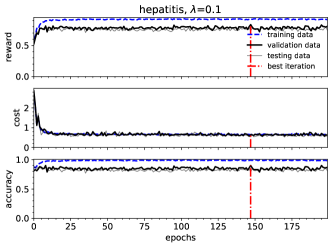
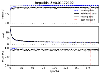
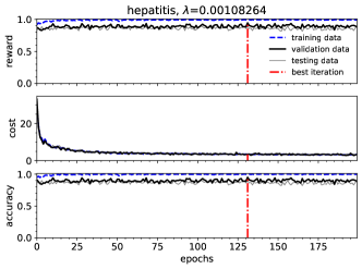
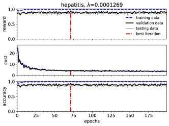
Figure 14: Convergence graphs for hepatitis dataset.

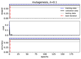
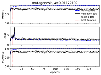
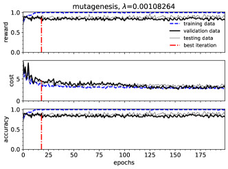
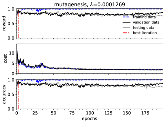
Figure 15: Convergence graphs for mutagenesis dataset.

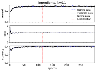
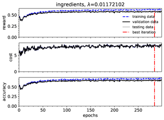
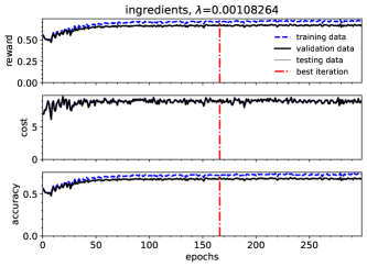
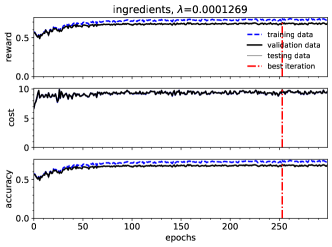
Figure 16: Convergence graphs for ingredients dataset.

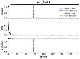
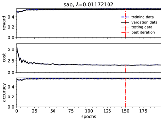
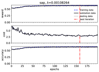
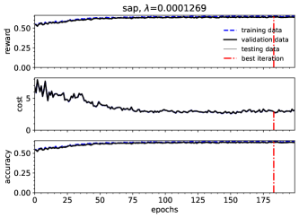
Figure 17: Convergence graphs for sap dataset.

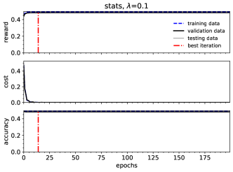
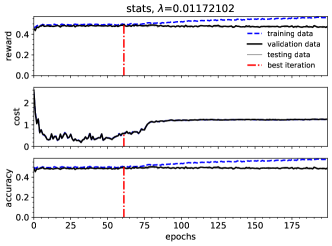
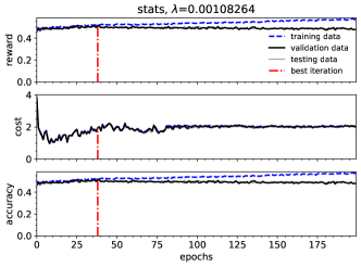
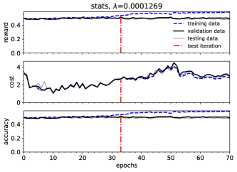
Figure 18: Convergence graphs for stats dataset.

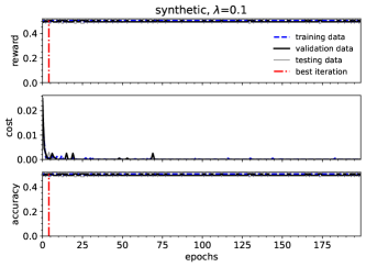
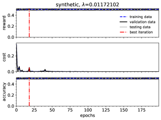
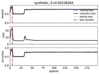
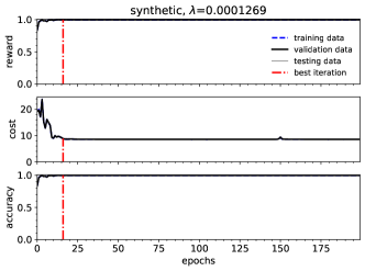
Figure 19: Convergence graphs for synthetic dataset.

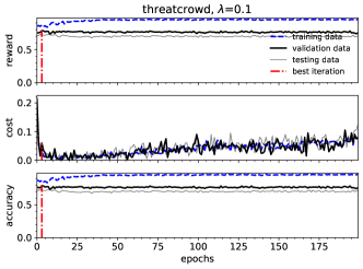
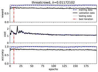
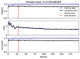
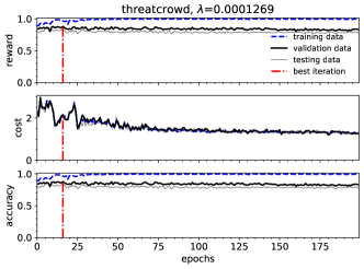
Figure 20: Convergence graphs for threatcrowd dataset.

References

- [1] G. Dulac-Arnold, L. Denoyer, P. Preux, and P. Gallinari, “Sequential approaches for learning datum-wise sparse representations,” Machine learning, vol. 89, no. 1-2, pp. 87–122, 2012.
- [2] J. Janisch, T. Pevný, and V. Lisý, “Classification with costly features using deep reinforcement learning,” in Proceedings of 33rd AAAI Conference on Artificial Intelligence, 2019.
- [3] ——, “Classification with costly features as a sequential decision-making problem,” Machine Learning, vol. 109, no. 8, pp. 1587–1615, 2020.
- [4] T. Pevný and P. Somol, “Discriminative models for multi-instance problems with tree structure,” in Proceedings of the 2016 ACM Workshop on Artificial Intelligence and Security. ACM, 2016, pp. 83–91.
- [5] F. Morin and Y. Bengio, “Hierarchical probabilistic neural network language model.” in Aistats, vol. 5. Citeseer, 2005, pp. 246–252.
- [6] Z. Xu, K. Weinberger, and O. Chapelle, “The greedy miser: learning under test-time budgets,” in Proceedings of the 29th International Coference on International Conference on Machine Learning. Omnipress, 2012, pp. 1299–1306.
- [7] M. Kusner, W. Chen, Q. Zhou, Z. Xu, K. Weinberger, and Y. Chen, “Feature-cost sensitive learning with submodular trees of classifiers,” in AAAI Conference on Artificial Intelligence, 2014, pp. 1939–1945.
- [8] Z. Xu, M. Kusner, K. Weinberger, and M. Chen, “Cost-sensitive tree of classifiers,” in International Conference on Machine Learning, 2013, pp. 133–141.
- [9] Z. Xu, M. Kusner, K. Weinberger, M. Chen, and O. Chapelle, “Classifier cascades and trees for minimizing feature evaluation cost,” Journal of Machine Learning Research, vol. 15, no. 1, pp. 2113–2144, 2014.
- [10] F. Nan, J. Wang, and V. Saligrama, “Feature-budgeted random forest,” in International Conference on Machine Learning, 2015, pp. 1983–1991.
- [11] ——, “Pruning random forests for prediction on a budget,” in Advances in Neural Information Processing Systems, 2016, pp. 2334–2342.
- [12] F. Nan and V. Saligrama, “Adaptive classification for prediction under a budget,” in Advances in Neural Information Processing Systems, 2017, pp. 4730–4740.
- [13] G. Contardo, L. Denoyer, and T. Artieres, “Recurrent neural networks for adaptive feature acquisition,” in International Conference on Neural Information Processing. Springer, 2016, pp. 591–599.
- [14] J. Wang, K. Trapeznikov, and V. Saligrama, “An lp for sequential learning under budgets,” in Artificial Intelligence and Statistics, 2014, pp. 987–995.
- [15] J. Wang, T. Bolukbasi, K. Trapeznikov, and V. Saligrama, “Model selection by linear programming,” in European Conference on Computer Vision. Springer, 2014, pp. 647–662.
- [16] Y. W. Liyanage, D.-S. Zois, and C. Chelmis, “Dynamic instance-wise joint feature selection and classification,” IEEE Transactions on Artificial Intelligence, 2021.
- [17] H. Shim, S. J. Hwang, and E. Yang, “Joint active feature acquisition and classification with variable-size set encoding,” in Advances in Neural Information Processing Systems, 2018, pp. 1375–1385.
- [18] Y. Li and J. Oliva, “Active feature acquisition with generative surrogate models,” in International Conference on Machine Learning. PMLR, 2021, pp. 6450–6459.
- [19] Y. Tang and S. Agrawal, “Discretizing continuous action space for on-policy optimization,” in Proceedings of the AAAI Conference on Artificial Intelligence, vol. 34, 2020, pp. 5981–5988.
- [20] Y.-E. Chen, K.-F. Tang, Y.-S. Peng, and E. Y. Chang, “Effective medical test suggestions using deep reinforcement learning,” arXiv preprint arXiv:1905.12916, 2019.
- [21] L. Metz, J. Ibarz, N. Jaitly, and J. Davidson, “Discrete sequential prediction of continuous actions for deep rl,” arXiv preprint arXiv:1705.05035, 2017.
- [22] J. Goodman, “Classes for fast maximum entropy training,” in 2001 IEEE International Conference on Acoustics, Speech, and Signal Processing. Proceedings (Cat. No. 01CH37221), vol. 1. IEEE, 2001, pp. 561–564.
- [23] J. Zhou, G. Cui, Z. Zhang, C. Yang, Z. Liu, and M. Sun, “Graph neural networks: A review of methods and applications,” arXiv preprint arXiv:1812.08434, 2018.
- [24] W. Hamilton, Z. Ying, and J. Leskovec, “Inductive representation learning on large graphs,” in Advances in Neural Information Processing Systems, 2017, pp. 1024–1034.
- [25] B. Perozzi, R. Al-Rfou, and S. Skiena, “Deepwalk: Online learning of social representations,” in Proceedings of the 20th ACM SIGKDD international conference on Knowledge discovery and data mining. ACM, 2014, pp. 701–710.
- [26] T. N. Kipf and M. Welling, “Semi-supervised classification with graph convolutional networks,” arXiv preprint arXiv:1609.02907, 2016.
- [27] V. Mnih, A. P. Badia, M. Mirza, A. Graves, T. Lillicrap, T. Harley, D. Silver, and K. Kavukcuoglu, “Asynchronous methods for deep reinforcement learning,” in International Conference on Machine Learning, 2016, pp. 1928–1937.
- [28] T. Pevný and P. Somol, “Using neural network formalism to solve multiple-instance problems,” in International Symposium on Neural Networks. Springer, 2017, pp. 135–142.
- [29] M. Zaheer, S. Kottur, S. Ravanbakhsh, B. Poczos, R. R. Salakhutdinov, and A. J. Smola, “Deep sets,” in Advances in neural information processing systems, 2017, pp. 3391–3401.
- [30] T. Pevný and V. Kovařík, “Approximation capability of neural networks on spaces of probability measures and tree-structured domains,” arXiv preprint arXiv:1906.00764, 2019.
- [31] Y. Zhang, Q. H. Vuong, K. Song, X.-Y. Gong, and K. W. Ross, “Efficient entropy for policy gradient with multidimensional action space,” arXiv preprint arXiv:1806.00589, 2018.
- [32] M. Damashek, “Gauging similarity with n-grams: Language-independent categorization of text,” Science, vol. 267, no. 5199, pp. 843–848, 1995.
- [33] I. Loshchilov and F. Hutter, “Decoupled weight decay regularization,” in International Conference on Learning Representations, 2018.
- [34] W. S. Cleveland, “Lowess: A program for smoothing scatterplots by robust locally weighted regression,” American Statistician, vol. 35, no. 1, p. 54, 1981.
- [35] Š. Mandlík, “Mapping the internet — modelling entity interactions in complex heterogeneous networks,” Master’s thesis, Czech technical university in Prague, 2020.
- [36] J. Motl and O. Schulte, “The CTU Prague relational learning repository,” arXiv preprint arXiv:1511.03086, 2015. [Online]. Available: https://relational.fit.cvut.cz/
- [37] J. L. Ba, J. R. Kiros, and G. E. Hinton, “Layer normalization,” arXiv preprint arXiv:1607.06450, 2016.