Enantiomeric excess determination based on nonreciprocal transition induced spectral line elimination

Abstract

The spontaneous emission spectrum of a multi-level atom or molecule with nonreciprocal transition is investigated. It is shown that the nonreciprocal transition can lead to the elimination of a spectral line in the spontaneous emission spectrum. As an application, we show that nonreciprocal transition arises from the phase-related driving fields in chiral molecules with cyclic three-level transitions, and the elimination of a spectral line induced by nonreciprocal transition provides us a method to determine the enantiomeric excess for the chiral molecules without requiring the enantio-pure samples.

I Introduction

Nonreciprocity is a very general concept that arises in many branches of physics, such as electronics, optics JalasNPT13 ; CalozPRAPP18 , acoustics MaznevaWM13 ; FleurySci14 , and condensed-matter physics AtalaNPy14 . Nonreciprocity means that some particles or waves exhibit different transmission properties when their sources and detectors are exchanged, such as the one-way electric conduction in the semiconductor p-n junctions. In a recent paper XWXuArx19 , some of us introduced the concept of nonreciprocity to investigate the transitions between different energy levels, and proposed a generic method to realize significant difference between the stimulated emission and absorption coefficients of two nondegenerate energy levels, which we refer to as nonreciprocal transition XWXuArx19 . The nonreciprocal transition can be used for many applications, such as single-photon nonreciprocal transporter XWXuArx19 , nonreciprocal phonon devices JZhangPRB15 ; YJiangPRAPP18 , and the echo cancellation in quantum memory LvovskyNPo09 and quantum measurements ClerkRMP10 .

In this paper, we will study the spontaneous emission of a multi-level atom or molecule with nonreciprocal transition. The spontaneous emission spectrum emitted from an atom or molecule shows a valuable insight into the behaviour of transitions between different energy levels SYZhuPRA95 ; SYZhuPRL96 . We find that the nonreciprocal transition can be reflected with spectral line elimination in the spontaneous emission spectra, which provides us a very simple way to test nonreciprocal transition in experiment.

On the other hand, chirality is important in chemistry and biology for many chemical and biological processes are chirality-dependent BuschEls06 . But the chiral discrimination and separation remain challenging works under the existing experimental technical conditions. Some spectroscopic methods have been developed to determine enantiomeric excess, such as circular dichroism StephensJPC85 ; FanoodNC15 , Raman optical activity YHeAS11 ; BegzjavOE19 , and spectroscopy for a cyclic three-level model AnsariPRA90 ; YXLiuPRL05 ; CYePRA18 based on quantum interference effects WZJiaPRA11 , three-wave mixing  HirotaPJASB12 ; PattersonNat13 ; PattersonPRL13 ; PattersonPCCP14 ; ShubertACIE14 ; LobsigerJPCL15 ; ShubertJPCL15 ; ShubertJCP15 ; EibenbergerPRL17 ; PerezACIE17 ; LeibscherJCP19 ; KochRMP19 , ac Stark effect CYePRA19 , or deflection effect YYChenArx19 . In addition, many methods were proposed to achieve inner-state separating KralPRL01 ; YLiPRA08 ; WZJiaJPB10 ; LehmannJCP18 ; VitanovPRL19 ; CYePRA19 ; CYearX19 ; JLWuarX19 or spatially separating YLiPRL07 ; XLiJCP10 ; JacobJCP12 ; BrandPRL18 ; MilnerPRL19 ; SuzukiPRA19 molecules of different chiralities, and enantioconversion of chiral mixtures ShapiroPRL00 ; BrumerPRA01 ; GerbasiJCP01 ; KralPRL03 ; FrishmanJPB04 ; CYeArx19 .

In the latter part of this paper, we apply the general theory of the spontaneous emission of multi-level systems to the chiral molecules. We show that nonreciprocal transition arises from the phase-related driving fields in chiral molecules with cyclic three-level transitions and the appearance of spectral line elimination in the spontaneous emission spectra around some resonant frequencies is chirality-dependent. Therefore, the enantiomeric excess can be determined by measuring the spontaneous emission spectra of chiral molecules. Different from the traditional methods of enantiomeric excess determination StephensJPC85 ; FanoodNC15 ; YHeAS11 , the spectral line elimination in the spontaneous emission spectrum induced by nonreciprocal transition provides us another method to determine the enantiomeric excess for chiral molecules without requiring the enantio-pure samples.

The remainder of this paper is organized as follows. In Sec. II, the basic theory for spontaneous emission spectrum of a general multi-level system with nonreciprocal transition is introduced. The time evolution of the populations and the corresponding spontaneous emission spectra of the multi-level system with nonreciprocal transition are investigated in detail in Sec. III. The application of the spontaneous emission spectra in determining the enantiomeric excess for chiral molecules are discussed in Sec. IV. Finally, a summary is given in Sec. V.

II Basic theory for spontaneous emission spectrum

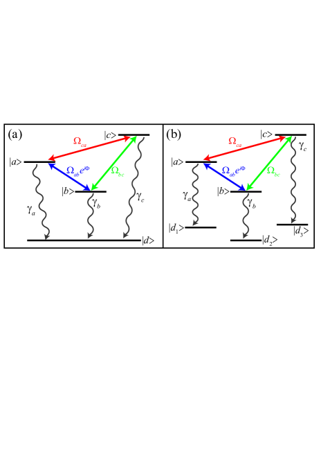
Figure 1: (Color online) Level diagram of an atom or molecule with cyclic transitions for the three upper levels ($|a\rangle$, $|b\rangle$ and $|c\rangle$), and they are coupled by the same vacuum modes to (a) the common lower level ($|d\rangle$), or (b) different lower levels ($|d_{1}\rangle$, $|d_{2}\rangle$ and $|d_{3}\rangle$).

We study the spontaneous emission of an atom or molecule with three upper levels ($|a\rangle$, $|b\rangle$, and $|c\rangle$), which are coupled to each other by three strong fields with frequencies ($\nu_{ab}$, $\nu_{cb}$, and $\nu_{ca}$), Rabi frequencies ($\Omega_{ab}$, $\Omega_{cb}$, and $\Omega_{ca}$) and phases ($\phi_{ab}$, $\phi_{cb}$, and $\phi_{ca}$). The spontaneous emission spectrum for the system will be derived for two different cases: (A) the three upper levels are coupled to one common lower level ($|d\rangle$) with the same vacuum modes, as shown in Fig. 1(a), or (B) the three upper levels are coupled to three different lower levels ($|d_{1}\rangle$, $|d_{2}\rangle$, and $|d_{3}\rangle$) respectively with the same vacuum modes, as shown in Fig. 1(b).

II.1 With one common lower level

Consider the three upper levels ($|a\rangle$, $|b\rangle$, and $|c\rangle$) coupled with one common lower level ($|d\rangle$) by the same vacuum modes. The interaction Hamiltonian of the system in the interaction picture can be written as ($\hbar=1$)

$$V = \Omega_{ab}e^{i\Phi}e^{i\Delta_{ab}t}\left|a\right\rangle\left\langle b\right|+\Omega_{cb}e^{i\Delta_{cb}t}\left|c\right\rangle\left\langle b\right|+\Omega_{ca}e^{i\Delta_{ca}t}\left|c\right\rangle\left\langle a\right|$$ (1)

$$+\sum_{k}\left[g_{k}^{ad}e^{i\left(\omega_{ad}-\omega_{k}\right)t}v_{k}\left|a\right\rangle\left\langle d\right|+g_{k}^{bd}e^{i\left(\omega_{bd}-\omega_{k}\right)t}v_{k}\left|b\right\rangle\left\langle d\right|+g_{k}^{cd}e^{i\left(\omega_{cd}-\omega_{k}\right)t}v_{k}\left|c\right\rangle\left\langle d\right|\right.$$

$$+\mathrm{H.c.},$$

where $\omega_{\sigma\sigma^{\prime}}$ $\left(\sigma,\sigma^{\prime}=a,b,c,d\right)$ are the frequency differences between levels $|\sigma\rangle$ and $|\sigma^{\prime}\rangle$, $\Delta_{\sigma\sigma^{\prime}}=\omega_{\sigma\sigma^{\prime}}-\nu_{\sigma\sigma^{\prime}}$ is the detuning of the driving fields, $v_{k}$ ($v_{k}^{\dagger}$) is the annihilation (creation) operator for the $k$th vacuum mode with frequency $\omega_{k}$, and $g_{k}^{\sigma d}$ is the coupling constant between the $k$th vacuum mode and the atomic transition from $|\sigma\rangle$ to $|d\rangle$. Here real $g_{k}^{\sigma d}$ is assumed, $k$ denotes both the momentum and polarization of the vacuum modes, and the total phase $\Phi=\phi_{ab}-\phi_{cb}+\phi_{ca}$ is obtained by redefining $e^{-i\phi_{cb}}|b\rangle\rightarrow|b\rangle$ and $e^{-i\phi_{ca}}|a\rangle\rightarrow|a\rangle$.

We assume the system is initially prepared in one of the upper levels, i.e., $|\psi(0)\rangle=|b\rangle|0\rangle$, where $|0\rangle$ denotes the vacuum state. The state vector at time $t$ can be written as

$$\left|\psi\left(t\right)\right\rangle=\left[A\left(t\right)\left|a\right\rangle+B\left(t\right)\left|b\right\rangle+C\left(t\right)\left|c\right\rangle+\sum_{k}D_{k}\left(t\right)v^{\dagger}_{k}\left|d\right\rangle\right]\left|0\right\rangle,$$ (2)

where the modulus squares of the coefficients $A(t)$, $B(t)$, $C(t)$ and $D_{k}(t)$ are the occupation probabilities in the corresponding state at time $t$. By using the Weisskopf-Wigner approximation, the dynamical behaviors for the coefficients are given by

$$\frac{d}{dt}A\left(t\right) = -\frac{\gamma_{a}}{2}A\left(t\right)-p_{ab}\frac{\sqrt{\gamma_{a}\gamma_{b}}}{2}e^{i\omega_{ab}t}B\left(t\right)-p_{ca}\frac{\sqrt{\gamma_{a}\gamma_{c}}}{2}e^{-i\omega_{ca}t}C\left(t\right)$$ (3)

$$-i\Omega_{ab}e^{i\Phi}e^{i\Delta_{ab}t}B\left(t\right)-i\Omega_{ca}e^{-i\Delta_{ca}t}C\left(t\right),$$

$$\frac{d}{dt}B\left(t\right) = -\frac{\gamma_{b}}{2}B\left(t\right)-p_{ab}\frac{\sqrt{\gamma_{a}\gamma_{b}}}{2}e^{-i\omega_{ab}t}A\left(t\right)-p_{cb}\frac{\sqrt{\gamma_{b}\gamma_{c}}}{2}e^{-i\omega_{cb}t}C\left(t\right)$$ (4)

$$-i\Omega_{bc}e^{-i\Delta_{cb}t}C\left(t\right)-i\Omega_{ab}e^{-i\Phi}e^{-i\Delta_{ab}t}A\left(t\right),$$

$$\frac{d}{dt}C\left(t\right) = -\frac{\gamma_{c}}{2}C\left(t\right)-p_{ca}\frac{\sqrt{\gamma_{a}\gamma_{c}}}{2}e^{i\omega_{ca}t}A\left(t\right)-p_{cb}\frac{\sqrt{\gamma_{c}\gamma_{b}}}{2}e^{i\omega_{cb}t}B\left(t\right)$$ (5)

$$-i\Omega_{ca}e^{i\Delta_{ca}t}A\left(t\right)-i\Omega_{bc}e^{i\Delta_{cb}t}B\left(t\right),$$

$$\frac{d}{dt}D_{k}\left(t\right)=-ig_{k}^{ad}e^{-i\left(\omega_{ad}-\omega_{k}\right)t}A\left(t\right)-ig_{k}^{bd}e^{-i\left(\omega_{bd}-\omega_{k}\right)t}B\left(t\right)-ig_{k}^{cd}e^{-i\left(\omega_{cd}-\omega_{k}\right)t}C\left(t\right),$$ (6)

where $\gamma_{a}=[2\pi(g^{ad}_{k})^{2}\rho(\omega_{k})]_{\omega_{k}=\omega_{ad}}$, $\gamma_{b}=[2\pi(g_{k}^{bd})^{2}\rho(\omega_{k})]_{\omega_{k}=\omega_{bd}}$ and $\gamma_{c}=[2\pi(g_{k}^{cd})^{2}\rho(\omega_{k})]_{\omega_{k}=\omega_{cd}}$ are the decay rates, $\rho(\omega_{k})$ is the mode density, $p_{\sigma\sigma^{\prime}}=\vec{\mu}_{\sigma}\cdot\vec{\mu}_{\sigma^{\prime}}/(|\vec{\mu}_{\sigma}|\cdot|\vec{\mu}_{\sigma^{\prime}}|)$ and $\vec{\mu}_{\sigma}$ ($\vec{\mu}_{\sigma^{\prime}}$) is the the dipole moment of the transition from $|\sigma\rangle$ ($|\sigma^{\prime}\rangle$) to $|d\rangle$ ($\sigma,\sigma^{\prime}=a,b,c$). The coupling terms with $p_{\sigma\sigma^{\prime}}$ is induced by the decays from different upper levels ($|\sigma\rangle$ and $|\sigma^{\prime}\rangle$) to the common lower level $|d\rangle$, which can result in spontaneous emission cancellation and spectral line elimination SYZhuPRA95 ; SYZhuPRL96 . However, here $\{\omega_{ab},\omega_{ca},\omega_{cb}\}\gg\{\gamma_{a},\gamma_{b},\gamma_{c},\Delta_{ab},\Delta_{ca},\Delta_{cb}\}$ are assumed so that the high-frequency oscillating terms (i.e., the decay induced coupling terms with $p_{\sigma\sigma^{\prime}}\frac{\sqrt{\gamma_{\sigma}\gamma_{\sigma^{\prime}}}}{2}e^{\pm i\omega_{\sigma\sigma^{\prime}}t}$) in Eqs. (3)-(5) can be neglected, and the dynamical equations are simplified as

$$\frac{d}{dt}A\left(t\right)=-\frac{\gamma_{a}}{2}A\left(t\right)-i\Omega_{ab}e^{i\Phi}e^{i\Delta_{ab}t}B\left(t\right)-i\Omega_{ca}e^{-i\Delta_{ca}t}C\left(t\right),$$ (7)

$$\frac{d}{dt}B\left(t\right)=-\frac{\gamma_{b}}{2}B\left(t\right)-i\Omega_{bc}e^{-i\Delta_{cb}t}C\left(t\right)-i\Omega_{ab}e^{-i\Phi}e^{-i\Delta_{ab}t}A\left(t\right),$$ (8)

$$\frac{d}{dt}C\left(t\right)=-\frac{\gamma_{c}}{2}C\left(t\right)-i\Omega_{ca}e^{i\Delta_{ca}t}A\left(t\right)-i\Omega_{bc}e^{i\Delta_{cb}t}B\left(t\right).$$ (9)

For convenience of calculations, let us define $\widetilde{B}\left(t\right)\equiv e^{i\Delta_{ab}t}B\left(t\right)$ and $\widetilde{C}\left(t\right)\equiv e^{-i\Delta_{ca}t}C\left(t\right)$ and make the assumption of three-photon resonance $\Delta_{ca}+\Delta_{ab}=\Delta_{cb}$, then we get a dynamical equations with constant coefficients as

$$\frac{dA\left(t\right)}{dt}=-\frac{\gamma_{a}}{2}A\left(t\right)-i\Omega_{ab}e^{i\Phi}\widetilde{B}\left(t\right)-i\Omega_{ca}\widetilde{C}\left(t\right),$$ (10)

$$\frac{d\widetilde{B}\left(t\right)}{dt}=-\left(\frac{\gamma_{b}}{2}-i\Delta_{ab}\right)\widetilde{B}\left(t\right)-i\Omega_{bc}\widetilde{C}\left(t\right)-i\Omega_{ab}e^{-i\Phi}A\left(t\right),$$ (11)

$$\frac{d\widetilde{C}\left(t\right)}{dt}=-\left(\frac{\gamma_{c}}{2}+i\Delta_{ca}\right)\widetilde{C}\left(t\right)-i\Omega_{ca}A\left(t\right)-i\Omega_{bc}\widetilde{B}\left(t\right).$$ (12)

All the following calculations and discussions on the occupation probabilities are based on Eqs. (10)-(12).

In the following, we will use the Laplace transform method to solve the dynamic equations. By taking the Laplace transform, i.e., $\overline{O}\left(s\right)=\int_{0}^{+\infty}O\left(t\right)e^{-st}dt$, of Eqs. (10)-(12), with the initial condition $\Psi_{0}=\left[A\left(0\right),\widetilde{B}\left(0\right),\widetilde{C}\left(0\right)\right]^{T}$, we get

$$\overline{\Psi}=M^{-1}\Psi_{0}$$ (13)

with $\overline{\Psi}=\left[\overline{A}\left(s\right),\overline{\widetilde{B}}\left(s\right),\overline{\widetilde{C}}\left(s\right)\right]^{T}$, and

$$M=\left(\begin{array}[]{ccc}s+\frac{\gamma_{a}}{2}&i\Omega_{ab}e^{i\Phi}&i\Omega_{ca}\\ i\Omega_{ab}e^{-i\Phi}&s+\frac{\gamma_{b}}{2}-i\Delta_{ab}&i\Omega_{bc}\\ i\Omega_{ca}&i\Omega_{bc}&s+\frac{\gamma_{c}}{2}+i\Delta_{ca}\end{array}\right).$$ (14)

The spontaneous emission spectrum of the system, $S\left(\omega\right)$, is the Fourier transform of

$$\left\langle E^{-}\left(t+\tau\right)E^{+}\left(t\right)\right\rangle_{t\rightarrow+\infty} \equiv \left\langle\psi\right|\sum_{k,k^{\prime}}v_{k}^{{\dagger}}e^{i\omega_{k}\left(t+\tau\right)}v_{k^{\prime}}e^{-i\omega_{k^{\prime}}t}\left|\psi\right\rangle_{t\rightarrow+\infty}$$ (15)

$$= \int_{-\infty}^{+\infty}\left|D_{k}\left(+\infty\right)\right|^{2}\rho\left(\omega_{k}\right)e^{i\omega_{k}\tau}d\omega_{k},$$

then we have $S\left(\omega_{k}\right)=\left|D_{k}\left(+\infty\right)\right|^{2}\rho\left(\omega_{k}\right)$, where $D_{k}\left(+\infty\right)$ is the long time behavior ($t\rightarrow+\infty$) of $D_{k}\left(t\right)$ and can be obtained by integrating time $t^{\prime}$ in Eq. (6) as

$$D_{k}\left(+\infty\right) = \int_{0}^{+\infty}\left[-ig_{k}^{ad}e^{-i\left(\omega_{ad}-\omega_{k}\right)t^{\prime}}A\left(t^{\prime}\right)-ig_{k}^{bd}e^{-i\left(\omega_{bd}-\omega_{k}+\Delta_{ab}\right)t^{\prime}}\widetilde{B}\left(t^{\prime}\right)-ig_{k}^{cd}e^{-i\left(\omega_{cd}-\omega_{k}-\Delta_{ca}\right)t^{\prime}}\widetilde{C}\left(t^{\prime}\right)\right]dt^{\prime}$$ (16)

$$= -ig_{k}^{ad}\overline{A}\left(-i\delta_{k}\right)-ig_{k}^{bd}\overline{\widetilde{B}}\left(-i\delta^{b}_{k}\right)-ig_{k}^{cd}\overline{\widetilde{C}}\left(-i\delta^{c}_{k}\right)$$

with the detunings $\delta_{k}\equiv\omega_{k}-\omega_{ad}$, $\delta^{b}_{k}\equiv\delta_{k}+\omega_{ab}-\Delta_{ab}$, $\delta^{c}_{k}\equiv\delta_{k}-\omega_{ca}+\Delta_{ca}$. Finally, the spontaneous emission spectrum is given by

$$S\left(\omega_{k}\right)=\frac{1}{2\pi}\left|\sqrt{\gamma_{a}}\overline{A}\left(-i\delta_{k}\right)+\sqrt{\gamma_{b}}\overline{\widetilde{B}}\left(-i\delta^{b}_{k}\right)+\sqrt{\gamma_{c}}\overline{\widetilde{C}}\left(-i\delta^{c}_{k}\right)\right|^{2},$$ (17)

with $\overline{A}\left(s\right)$, $\overline{\widetilde{B}}\left(s\right)$, and $\overline{\widetilde{C}}\left(s\right)$ given by Eq. (13).

II.2 With three different lower levels

In the case with three different lower levels, the interaction Hamiltonian of the system is given in the interaction picture by

$$V^{\prime} = \Omega_{ab}e^{i\Phi}e^{i\Delta_{ab}t}\left|a\right\rangle\left\langle b\right|+\Omega_{bc}e^{i\Delta_{cb}t}\left|c\right\rangle\left\langle b\right|+\Omega_{ca}e^{i\Delta_{ca}t}\left|c\right\rangle\left\langle a\right|$$ (18)

$$+\sum_{k}\left[g_{k}^{ad_{1}}e^{i\left(\omega_{ad_{1}}-\omega_{k}\right)t}v_{k}\left|a\right\rangle\left\langle d_{1}\right|+g_{k}^{bd_{2}}e^{i\left(\omega_{bd_{2}}-\omega_{k}\right)t}v_{k}\left|b\right\rangle\left\langle d_{2}\right|+g_{k}^{cd_{3}}e^{i\left(\omega_{cd_{3}}-\omega_{k}\right)t}v_{k}\left|c\right\rangle\left\langle d_{3}\right|\right]$$

$$+\mathrm{H.c.},$$

where $\omega_{\sigma d_{j}}$ denote the frequency differences between levels $|\sigma\rangle$ $\left(\sigma=a,b,c\right)$ and $|d_{j}\rangle$ ($j=1,2,3$), and $g_{k}^{\sigma d_{j}}$ is the coupling constant between the $k$th vacuum mode and the atomic transition from $|\sigma\rangle$ to $|d_{j}\rangle$. The state vector for the system at time $t$ can be written as

$$\left|\psi^{\prime}\left(t\right)\right\rangle=\left[A\left(t\right)\left|a\right\rangle+B\left(t\right)\left|b\right\rangle+C\left(t\right)\left|c\right\rangle\right]\left|0\right\rangle+\sum_{j=1,2,3}\sum_{k}D_{j,k}\left(t\right)\left|d_{j}\right\rangle\left|1\right\rangle_{k}.$$ (19)

By substituting the Hamiltonian and state vector into the Schrödinger equation and using the Weisskopf-Wigner approximation, the dynamic equations of the coefficients [$A(t)$, $B(t)$, and $C(t)$] are obtained and they have the same forms as those given by Eqs. (7)-(9), with the decay rates replaced by $\gamma^{\prime}_{a}=[2\pi(g^{ad_{1}}_{k})^{2}\rho(\omega_{k})]_{\omega_{k}=\omega_{ad_{1}}}$, $\gamma^{\prime}_{b}=[2\pi(g_{k}^{bd_{2}})^{2}\rho(\omega_{k})]_{\omega_{k}=\omega_{bd_{2}}}$, and $\gamma^{\prime}_{c}=[2\pi(g_{k}^{cd_{3}})^{2}\rho(\omega_{k})]_{\omega_{k}=\omega_{cd_{3}}}$. The spontaneous emission spectrum is obtained as $S\left(\omega_{k}\right)=\sum_{j=1,2,3}\left|D_{j,k}\left(+\infty\right)\right|^{2}\rho\left(\omega_{k}\right)$, where

$$D_{1,k}\left(+\infty\right)=-ig_{k}^{ad_{1}}\overline{A}\left(-i\delta_{k}^{\prime}\right),$$ (20)

$$D_{2,k}\left(+\infty\right)=-ig_{k}^{bd_{2}}\overline{\widetilde{B}}\left(-i\delta_{k}^{b\prime}\right),$$ (21)

$$D_{3,k}\left(+\infty\right)=-ig_{k}^{cd_{3}}\overline{\widetilde{C}}\left(-i\delta_{k}^{c\prime}\right),$$ (22)

the coefficients [$\overline{A}\left(s\right)$, $\overline{\widetilde{B}}\left(s\right)$, and $\overline{\widetilde{C}}\left(s\right)$] are given by Eq. (13), and the detunings are defined by $\delta_{k}^{\prime}\equiv\omega_{k}-\omega_{ad_{1}}$, $\delta_{k}^{b\prime}\equiv\omega_{k}-\omega_{bd_{2}}-\Delta_{ab}=\delta_{k}^{\prime}+\omega_{ab}^{\prime}-\Delta_{ab}$, $\delta_{k}^{c\prime}\equiv\omega_{k}-\omega_{cd_{3}}+\Delta_{ca}=\delta_{k}^{\prime}-\omega_{ca}^{\prime}+\Delta_{ca}$, with $\omega_{ab}^{\prime}\equiv\omega_{ad_{1}}-\omega_{bd_{2}}$, $\omega_{ca}^{\prime}\equiv\omega_{cd_{3}}-\omega_{ad_{1}}$. Thus, the spontaneous emission spectrum for the case with three different lower levels can be specifically expressed as

$$S\left(\omega_{k}\right)=\frac{1}{2\pi}\left\{\gamma_{a}\left|\overline{A}\left(-i\delta_{k}^{\prime}\right)\right|^{2}+\gamma_{b}\left|\overline{\widetilde{B}}\left(-i\delta_{k}^{b\prime}\right)\right|^{2}+\gamma_{c}\left|\overline{\widetilde{C}}\left(-i\delta_{k}^{c\prime}\right)\right|^{2}\right\}.$$ (23)

For comparison with the case of one common lower level given by Eq. (17) in the following, we assume that $\omega_{ad_{1}}=\omega_{ad}$, $\omega_{bd_{2}}=\omega_{bd}$ and $\omega_{cd_{3}}=\omega_{cd}$, i.e., the three lower levels $|d_{j}\rangle$ ($j=1,2,3$) are degenerate, so that we have $\delta_{k}^{\prime}=\delta_{k}$, $\omega_{ab}^{\prime}=\omega_{ab}$, $\omega_{ca}^{\prime}=\omega_{ca}$, $\delta_{k}^{b\prime}=\delta^{b}_{k}$, $\delta_{k}^{c\prime}=\delta^{c}_{k}$, $\gamma^{\prime}_{a}=\gamma_{a}$, $\gamma^{\prime}_{b}=\gamma_{b}$, and $\gamma^{\prime}_{c}=\gamma_{c}$. However, we should point out that this assumption does not bring significant differences in physical appearance except the positions of resonance peaks in the spectra.

III Nonreciprocal transition and the spontaneous emission spectra

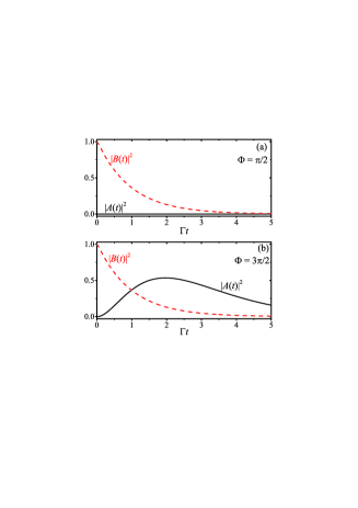
Figure 2: (Color online) The populations $|A\left(t\right)|^{2}$ (black solid curve) and $|B\left(t\right)|^{2}$ (red dashed curve) are plotted as functions of the time $\Gamma t$ for: (a) $\Phi=\pi/2$ and (b) $\Phi=3\pi/2$. The initial conditions are $A\left(0\right)=C\left(0\right)=0$ and $B\left(0\right)=1$. The other parameters are $\gamma_{a}=\gamma_{b}=\Gamma/100$, $\gamma_{c}=100\Gamma$, $\Omega_{ab}=\Gamma/2$, $\Omega_{ca}=\Omega_{bc}=5\Gamma$, $\Delta_{cb}=\Delta_{ca}=\Delta_{ab}=0$.

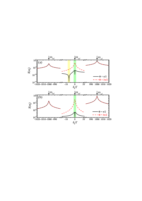
Figure 3: (Color online) The spontaneous emission spectra for the three upper levels ($|a\rangle$, $|b\rangle$, and $|c\rangle$) coupled by the same vacuum modes to (a) the common lower level ($|d\rangle$), or (b) different lower levels ($|d_{1}\rangle$, $|d_{2}\rangle$, and $|d_{3}\rangle$). The system is initially in level $|b\rangle$. The black solid curves are for phase $\Phi=\pi/2$ and the red dashed curves for $\Phi=3\pi/2$. The other parameters are $\gamma_{a}=\gamma_{b}=\Gamma/100$, $\gamma_{c}=100\Gamma$, $\Omega_{ab}=\Gamma/2$, $\Omega_{ca}=\Omega_{bc}=5\Gamma$, $\Delta_{cb}=\Delta_{ca}=\Delta_{ab}=0$, and $\omega_{ab}=\omega_{ca}=10^{3}\Gamma$.

First, let us investigate the time evolution of the upper-level populations with the system initially in level $|b\rangle$. The populations $|A\left(t\right)|^{2}$ (black solid curve) and $|B\left(t\right)|^{2}$ (red dashed curve) obtained from Eqs. (10)-(12) are plotted as functions of the time $t$ in Fig. 2. The population can transfer from the level $|b\rangle$ to level $|a\rangle$ for $\Phi=3\pi/2$, but almost no population will transfer from the level $|b\rangle$ to level $|a\rangle$ when $\Phi=\pi/2$, which agrees with the result given in Ref. XWXuArx19 . It has been shown in Ref. XWXuArx19 that the transition probability for $|b\rangle\rightarrow|a\rangle$ is different from the one for $|a\rangle\rightarrow|b\rangle$ when $\Phi\neq n\pi$ ($n$ is an integer), i.e., the transitions between levels $|b\rangle$ and $|a\rangle$ are nonreciprocal. As the decay induced coupling terms with $p_{\sigma\sigma^{\prime}}\frac{\sqrt{\gamma_{\sigma}\gamma_{\sigma^{\prime}}}}{2}e^{\pm i\omega_{\sigma\sigma^{\prime}}t}$) in Eqs. (3)-(5) are high-frequency oscillating terms and neglected safely under the assumption $\{\omega_{ab},\omega_{ca},\omega_{cb}\}\gg\{\gamma_{a},\gamma_{b},\gamma_{c},\Delta_{ab},\Delta_{ca},\Delta_{cb}\}$, the time evolutions of the upper-level populations are the same for both the two cases with one common or three different lower levels.

The nonreciprocal transitions can be observed by measuring the spontaneous emission spectra of the system. When $\Phi=3\pi/2$, as the population can transfer from the level $|b\rangle$ to level $|a\rangle$, there should be a peak around the resonant frequency $\omega_{ad}$. Instead, there is almost no population transferring from the level $|b\rangle$ to level $|a\rangle$ when $\Phi=\pi/2$, so that the peak around the frequency $\omega_{ad}$ will be eliminated (i.e., a dip should appear at there). In Fig. 3, the spontaneous emission spectra of the system are plotted for the three upper levels ($|a\rangle$, $|b\rangle$, and $|c\rangle$) coupled by the same vacuum modes to (a) the common lower level ($|d\rangle$), or (b) different lower levels ($|d_{1}\rangle$, $|d_{2}\rangle$, and $|d_{3}\rangle$). The black solid curves are for phase $\Phi=\pi/2$ and the red dashed curves for $\Phi=3\pi/2$. As expected for the spectra in both Figs. 3(a) and 3(b), there is a peak at the transition frequency $\omega_{ad}$ when $\Phi=3\pi/2$ or a dip when $\Phi=\pi/2$. Comparing the curves of Fig. 3(a) and Fig. 3(b), we find that there is another dip around $\delta_{k}/\Gamma=-6.7$ in the spectrum of the system with one common lower level when $\Phi=\pi/2$, which is induced by destructive interference between different decay paths to one common lower level SYZhuPRA95 ; SYZhuPRL96 .

IV Spontaneous emission spectra of chiral molecules

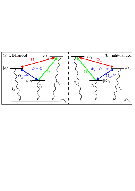
Figure 4: (Color online) Level diagram of a chiral molecule with cyclic transitions for the three upper levels ($|a\rangle_{Q}$, $|b\rangle_{Q}$ and $|c\rangle_{Q}$), and they are coupled by the same vacuum modes to the common lower level ($|d\rangle_{Q}$): (a) $Q=L$ for left-handed chiral states and (b) $Q=R$ for right-handed chiral states.

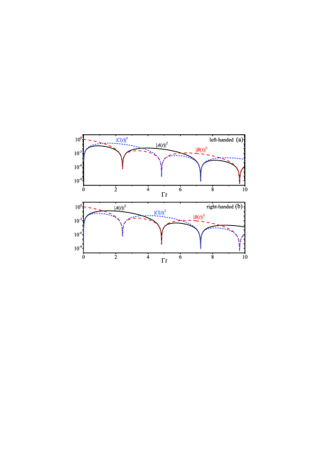
Figure 5: (Color online) The populations $|A\left(t\right)|^{2}$ (black solid curve), $|B\left(t\right)|^{2}$ (red dashed curve) and $|C\left(t\right)|^{2}$ (blue dot curve) are plotted as functions of the time $\Gamma t$ for: (a) left-handed molecules and (b) right-handed molecules. The initial conditions are $A\left(0\right)=C\left(0\right)=0$ and $B\left(0\right)=1$. The other parameters are $\gamma_{a}=\gamma_{b}=\gamma_{c}=\Gamma$, $\Omega_{ab}=\Omega_{ca}=\Omega_{bc}=\Gamma/2$, $\Delta_{cb}=\Delta_{ca}=\Delta_{ab}=0$, and $\Phi=\pi/2$.

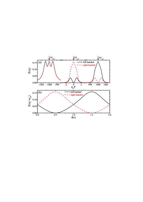
Figure 6: (Color online) The spontaneous emission spectra for a (left-handed or right-handed) chiral molecule with three upper levels ($|a\rangle_{Q}$, $|b\rangle_{Q}$ and $|c\rangle_{Q}$) coupled by the same vacuum modes to a common lower level ($|d\rangle_{Q}$). The molecule is initially in level $|b\rangle_{Q}$. The black solid curves are for the ($Q=L$) left-handed molecule and the red dashed curves for the ($Q=R$) right-handed molecule. (a) The spontaneous emission spectra versus $\delta_{k}$ for $\Phi=\pi/2$; (b) the spontaneous emission spectra versus $\Phi$ for $\omega_{k}=\omega_{ad}$. The other parameters are $\gamma_{a}=\gamma_{b}=\gamma_{c}=\Gamma$, $\Omega_{ab}=\Omega_{ca}=\Omega_{bc}=\Gamma/2$, $\Delta_{cb}=\Delta_{ca}=\Delta_{ab}=0$, and $\omega_{ab}=\omega_{ca}=10^{3}\Gamma$.

As an important application, we will discuss how to realize the determination of enantiomeric excess based on the spectral line elimination in the spontaneous emission spectra of chiral molecules. Our method is based on the model of chiral molecules with cyclic-transition three upper levels coupled with one common lower level by the same vacuum modes, as shown in Fig. 4, where $|a\rangle_{Q}$, $|b\rangle_{Q}$, $|c\rangle_{Q}$, and $|d\rangle_{Q}$ ($Q=L,R$) are the inner states of the left- and right-handed molecules. Both the models of left- and right-handed molecules can be described by the Hamiltonian given in Eq. (1) with $\Phi=\Phi_{L}$ for left-handed molecules and $\Phi=\Phi_{R}-\pi$ for right-handed molecules.

Let the chiral molecule initially be in level $|b\rangle_{Q}$. The time evolution of the populations in the three upper levels is shown in Fig. 5. For the left-handed molecule, the population is transferred from $|b\rangle_{L}$ to $|c\rangle_{L}$ first, then to $|a\rangle_{L}$, and last back to $|b\rangle_{L}$, with the maximum population decaying exponentially. Conversely, the population of the right-handed molecule is transferred from $|b\rangle_{L}$ to $|a\rangle_{L}$ first, then to $|c\rangle_{L}$, and last back to $|b\rangle_{L}$, with the maximum population decaying exponentially also. The chirality-dependent population transferring can be used for inner-state enantio-separation KralPRL01 ; KralPRL03 ; YLiPRA08 ; WZJiaJPB10 ; LehmannJCP18 ; VitanovPRL19 ; CYePRA19 ; CYearX19 ; JLWuarX19 . We note that the similar cyclic transitions between three levels have been observed in a ring with three transmon superconducting qubits RoushanNPy17 and a single spin under closed-contour interaction BarfussNPy18 . Nevertheless, the exponential decay of the maximum population is one ingredient for nonreciprocal transition between the three upper levels, and the direction of the transition is chirality-dependent. In Fig. 5, there is much more population transferred from $|b\rangle_{L}$ to $|c\rangle_{L}$ than that from $|b\rangle_{L}$ to $|a\rangle_{L}$ for left-handed molecules, and much more population transferred from $|b\rangle_{L}$ to $|a\rangle_{L}$ than that from $|b\rangle_{L}$ to $|c\rangle_{L}$ for right-handed molecules.

The nonreciprocal transition in the chiral molecules can be reflected in the spontaneous emission spectra. The spontaneous emission spectra for chiral molecules are plotted as a function of detuning $\delta_{k}$ in Fig. 6(a) with the black solid curves for left-handed molecules and the red dashed curves for right-handed molecules when $\Phi=\pi/2$. The most obvious difference between the two curves is there is one peak (with value $S_{L}$) at transition frequency $\omega_{cd}$ for left-handed molecules, but the peak is eliminated and a dip appears for right-handed molecules. By contrast, there is one peak (with value $S_{R}$) at transition frequency $\omega_{ad}$ for right-handed molecules, but the peak is eliminated for left-handed molecules. Then, the strengths of the spontaneous emission spectra of a chiral mixture, $S_{M}(\omega)$, at frequencies $\omega_{cd}$ and $\omega_{ad}$ are proportional to the molecule numbers of the two enantiomers, respectively,

$$S_{M}(\omega_{cd})\approx N_{L}S_{L},$$ (24)

$$S_{M}(\omega_{ad})\approx N_{R}S_{R},$$ (25)

where $N_{L}$ ($N_{R}$) is the number of left-handed (right-handed) molecules. For the enantiomeric excess of a chiral mixture defined by $\varepsilon\equiv(N_{L}-N_{R})/(N_{L}+N_{R})$, the enantiomeric excess can be determined by

$$\varepsilon=\frac{S_{M}(\omega_{cd})-\eta S_{M}(\omega_{ad})}{S_{M}(\omega_{cd})+\eta S_{M}(\omega_{ad})}$$ (26)

with the coefficient $\eta\equiv S_{L}/S_{R}$. Here, we have $\eta\approx 1$ with the parameters used in Figs. 5 and 6. In addition, the spontaneous emission spectra for chiral molecules show a sinusoidal dependence on the phase $\Phi$, as shown in Fig. 6(b). $\Phi=\pi/2$ and $\Phi=3\pi/2$ are two optimal phases to make the determination of enantiomeric excess mostly efficiently.

V Conclusions

In conclusion, we have studied the spontaneous emission spectrum of a multi-level system with nonreciprocal transition. Spectral line elimination appears in the spectra when there is almost no population transferring in one of the transition directions for nonreciprocal transition. The spectral line elimination induced by nonreciprocal transition provides us a method to determine the enantiomeric excess for the chiral molecules without requiring the enantio-pure samples. When the spectral line elimination appears at some resonant frequencies for molecules with one chirality, the strengths of the spontaneous emission spectra at that frequencies are proportional to the numbers of the molecules with the opposite chirality, so the enantiomeric excess can be determined by measuring the strengths of the spontaneous emission spectra at these frequencies.

Acknowledgement

X.-W.X. is supported by the National Natural Science Foundation of China (NSFC) under Grant No. 11604096, and the Key Program of Natural Science Foundation of Jiangxi Province, China under Grant No. 20192ACB21002. Y.L. is supported by National Key R&D Program of China under Grant No. 2016YFA0301200, and NSFC under Grants No. 11774024, No. U1930402, and No. U1730449. A.-X.C. is supported by NSFC under Grant No. 11775190.

References

• (1) D. Jalas, A. Petrov, M. Eich, W. Freude, S. Fan, Z. Yu, R. Baets, M. Popović, A. Melloni, J. D. Joannopoulos, M. Vanwolleghem, C. R. Doerr, and H. Renner, What is - and what is not - an optical isolator, Nat. Photon. 7, 579 (2013).
• (2) C. Caloz, A. Alù, S. Tretyakov, D. Sounas, K. Achouri, and Z.-L. Deck-Léger, Electromagnetic Nonreciprocity, Phys. Rev. Applied 10, 047001 (2018).
• (3) A. A. Mazneva, A. G. Every, and O. B. Wright, Reciprocity in reflection and transmission: What is a ‘phonon diode’?, Wave Motion 50, 776 (2013).
• (4) R. Fleury, D. L. Sounas, C. F. Sieck, M. R. Haberman, and A. Alù, Sound Isolation and Giant Linear Nonreciprocity in a Compact Acoustic Circulator, Science 343, 516 (2014).
• (5) M. Atala, M. Aidelsburger, M. Lohse, J. T. Barreiro, B. Paredes, and I. Bloch, Observation of chiral currents with ultracold atoms in bosonic ladders, Nat. Phys. 10, 588 (2014).
• (6) X. W. Xu, Y. J. Zhao, H. Wang, A. X. Chen, and Y. X. Liu, Nonreciprocal transition between two nondegenerate energy levels, arXiv:1908.08323 [quant-ph].
• (7) J. Zhang, B. Peng, S. K. Özdemir, Y. X. Liu, H. Jing, X. Y. Lü, Y. L. Liu, L. Yang, and F. Nori, Giant nonlinearity via breaking parity-time symmetry: A route to low-threshold phonon diodes, Phys. Rev. B 92, 115407 (2015).
• (8) Y. Jiang, S. Maayani, T. Carmon, F. Nori, and H. Jing, Nonreciprocal phonon laser, Phys. Rev. Appl. 10, 064037 (2018).
• (9) A. I. Lvovsky, B. C. Sanders, and W. Tittel, Optical quantum memory, Nat. Photonics 3, 706 (2009).
• (10) A. A. Clerk, M. H. Devoret, S. M. Girvin, F. Marquardt, and R. J. Schoelkopf, Introduction to quantum noise, measurement, and amplification, Rev. Mod. Phys. 82, 1155 (2010).
• (11) S. Y. Zhu, R. C. F. Chan, and C. P. Lee, Spontaneous emission from a three-level atom, Phys. Rev. A 52, 710 (1995).
• (12) S. Y. Zhu and M. O. Scully, Spectral Line Elimination and Spontaneous Emission Cancellation via Quantum Interference, Phys. Rev. Lett. 76, 388 (1996).
• (13) K. W. Busch and M. A. Busch (eds), Chiral Analysis (Elsevier, 2006).
• (14) P. J. Stephens, Theory of vibrational circular dichroism, J. Phys. Chem. 89, 748 (1985).
• (15) M. M. R. Fanood, N. B. Ram, C. S. Lehmann, I. Powis, and M. H. M. Janssen, Enantiomer-specific analysis of multi-component mixtures by correlated electron imaging–ion mass spectrometry, Nat. Commun. 6, 7511 (2015).
• (16) Y. He, B. Wang, R. K. Dukor, and L. A. Nafie, Determination of Absolute Configuration of Chiral Molecules Using Vibrational Optical Activity: A Review, Appl. Spectrosc. 65, 699 (2011).
• (17) T. Kh. Begzjav, Z. Zhang, M. O. Scully, G. S. Agarwal, Enhanced signals from chiral molecules via molecular coherence, Opt. Express 27, 13965 (2019).
• (18) N. A. Ansari, J. Gea-Banacloche, and M. S. Zubairy, Phase-sensitive amplification in a three-level atomic system, Phys. Rev. A 41, 5179 (1990).
• (19) Y. X. Liu, J. Q. You, L. F. Wei, C. P. Sun, and F. Nori, Optical Selection Rules and Phase-Dependent Adiabatic State Control in a Superconducting Quantum Circuit, Phys. Rev. Lett. 95, 087001 (2005).
• (20) C. Ye, Q. Zhang, and Y. Li, Real single-loop cyclic three-level configuration of chiral molecules, Phys. Rev. A 98, 063401 (2018).
• (21) W. Z. Jia and L. F. Wei, Probing molecular chirality by coherent optical absorption spectra, Phys. Rev. A 84, 053849 (2011).
• (22) E. Hirota, Triple resonance for a three-level system of a chiral molecule, Proc. Jpn. Acad., Ser. B 88, 120 (2012).
• (23) D. Patterson, M. Schnell, and J. M. Doyle, Enantiomer-specific detection of chiral molecules via microwave spectroscopy, Nature (London) 497, 475 (2013).
• (24) D. Patterson and J. M. Doyle, Sensitive chiral analysis via microwave three-wave mixing, Phys. Rev. Lett. 111, 023008 (2013).
• (25) D. Patterson and M. Schnell, New studies on molecular chirality in the gas phase: enantiomer differentiation and determination of enantiomeric excess, Phys. Chem. Chem. Phys. 16, 11114 (2014).
• (26) V. A. Shubert, D. Schmitz, D. Patterson, J. M. Doyle, and M. Schnell, Identifying Enantiomers in Mixtures of Chiral Molecules with Broadband Microwave Spectroscopy, Angew. Chem. Int. Ed. 53, 1152 (2014).
• (27) S. Lobsiger, C. Pérez, L. Evangelisti, K. K. Lehmann, and B. H. Pate, Molecular Structure and Chirality Detection by Fourier Transform Microwave Spectroscopy, J. Phys. Chem. Lett. 6, 196 (2015).
• (28) V. A. Shubert, D. Schmitz, C. Pérez, C. Medcraft, A. Krin, S. R. Domingos, D. Patterson, and M. Schnell, Chiral Analysis Using Broadband Rotational Spectroscopy, J. Phys. Chem. Lett. 7, 341 (2015).
• (29) V. A. Shubert, D. Schmitz, C. Medcraft, A. Krin, D. Patterson, J. M. Doyle, and M. Schnell, Rotational spectroscopy and three-wave mixing of 4-carvomenthenol: A technical guide to measuring chirality in the microwave regime, J. Chem. Phys. 142, 214201 (2015).
• (30) S. Eibenberger, J. M. Doyle, and D. Patterson, Enantiomer-Specific State Transfer of Chiral Molecules, Phys. Rev. Lett. 118, 123002 (2017).
• (31) C. Perez, A. L. Steber, S. R. Domingos, A. Krin, D. Schmitz, and M. Schnell, Coherent Enantiomer-Selective Population Enrichment using Tailored Microwave Fields, Angew. Chem. Int. Ed. 56, 12512 (2017).
• (32) M. Leibscher, T. F. Giesen, and C. P. Koch, Principles of enantio-selective excitation in three-wave mixing spectroscopy of chiral molecules, J. Chem. Phys. 151, 014302 (2019).
• (33) C. P. Koch, M. Lemeshko, and D. Sugny, Quantum control of molecular rotation, Rev. Mod. Phys. 91, 035005 (2019).
• (34) C. Ye, Q. Zhang, Y. Y. Chen, and Y. Li, Determination of enantiomeric excess with chirality-dependent ac Stark effects in cyclic three-level models, Phys. Rev. A 100, 033411 (2019).
• (35) Y. Y. Chen, C. Ye, Q. Zhang, and Y. Li, Enantio-discrimination via light deflection effect, arXiv:1909.06923 [physics.optics].
• (36) P. Král and M. Shapiro, Cyclic Population Transfer in Quantum Systems with Broken Symmetry, Phys. Rev. Lett. 87, 183002 (2001).
• (37) Y. Li and C. Bruder, Dynamic method to distinguish between left- and right-handed chiral molecules, Phys. Rev. A 77, 015403 (2008).
• (38) W. Z. Jia and L. F. Wei, Distinguishing left- and right-handed molecules using two-step coherent pulses, J. Phys. B: At. Mol. Opt. Phys. 43, 185402 (2010).
• (39) K. K. Lehmann, Influence of spatial degeneracy on rotational spectroscopy: Three-wave mixing and enantiomeric state separation of chiral molecules, J. Chem. Phys. 149, 094201 (2018).
• (40) N. V. Vitanov and M. Drewsen, Highly Efficient Detection and Separation of Chiral Molecules through Shortcuts to Adiabaticity, Phys. Rev. Lett. 122, 173202 (2019).
• (41) C. Ye, Q. Zhang, and Y. Li, Static nonlinear Schrödinger equations for the achiral-chiral transitions of polar chiral molecules, Phys. Rev. A 99, 062703 (2019).
• (42) C. Ye, Q. Zhang, Y. Y. Chen, and Y. Li, Effective two-level models for highly efficient inner-state enantio-separation based on cyclic three-level systems of chiral molecules, Phys. Rev. A 100, 043403 (2019).
• (43) J. L. Wu, Y. Wang, J. Song, Y. Xia, S. L. Su, and Y. Y. Jiang, Robust and highly efficient discrimination of chiral molecules through three-mode parallel paths, Phys. Rev. A 100, 043413 (2019).
• (44) Y. Li, C. Bruder, and C. P. Sun, Generalized Stern-Gerlach Effect for Chiral Molecules, Phys. Rev. Lett. 99, 130403 (2007).
• (45) X. Li and M. Shapiro, Theory of the optical spatial separation of racemic mixtures of chiral molecules, J. Chem. Phys. 132, 194315 (2010).
• (46) A. Jacob and K. Hornberger, Effect of molecular rotation on enantioseparation, J. Chem. Phys. 137, 044313 (2012).
• (47) C. Brand, B. A. Stickler, C. Knobloch, A. Shayeghi, K. Hornberger, and M. Arndt, Conformer Selection by Matter-Wave Interference, Phys. Rev. Lett. 121, 173002 (2018).
• (48) A. A. Milner, J. A. M. Fordyce, I. MacPhail-Bartley, W. Wasserman, V. Milner, I. Tutunnikov, and I. Sh. Averbukh, Controlled Enantioselective Orientation of Chiral Molecules with an Optical Centrifuge, Phys. Rev. Lett. 122, 223201 (2019).
• (49) F. Suzuki, T. Momose, and S. Y. Buhmann, Stern-Gerlach separator of chiral enantiomers based on the Casimir-Polder potential, Phys. Rev. A 99, 012513 (2019).
• (50) M. Shapiro, E. Frishman, and P. Brumer, Coherently Controlled Asymmetric Synthesis with Achiral Light, Phys. Rev. Lett. 84, 1669 (2000).
• (51) P. Brumer, E. Frishman, and M. Shapiro, Principles of electric-dipole-allowed optical control of molecular chirality, Phys. Rev. A 65, 015401 (2001).
• (52) D. Gerbasi, M. Shapiro, and P. Brumer, Theory of enantiomeric control in dimethylallene using achiral light, J. Chem. Phys. 115, 5349 (2001).
• (53) P. Král, I. Thanopulos, M. Shapiro, and D. Cohen, Two-Step Enantio-Selective Optical Switch, Phys. Rev. Lett. 90, 033001 (2003).
• (54) E. Frishman, M. Shapiro, and P. Brumer, Optical purification of racemic mixtures by ’laser distillation’ in the presence of a dissipative bath, J. Phys. B: At. Mol. Opt. Phys. 37, 2811 (2004).
• (55) C. Ye, Quansheng Zhang, Yu-Yuan Chen, and Yong Li, Fast enantioconversion of chiral mixtures based on a four-level double-$\Delta$ model, arXiv:1911.07376 [physics.optics].
• (56) P. Roushan, C. Neill, A. Megrant, Y. Chen, R. Babbush, R. Barends, B. Campbell, Z. Chen, B. Chiaro, A. Dunsworth, A. Fowler, E. Jeffrey, J. Kelly, L. E., J. Mutus, P. J.J. O’Malley, M. Neeley, C. Quintana, D. Sank, A. Vainsencher, J. Wenner, T. White, E. Kapit, H. Neven, and J. Martinis, Chiral ground-state currents of interacting photons in a synthetic magnetic field, Nature Phys. 13, 146 (2017).
• (57) A. Barfuss, J. Kölbl, L. Thiel, J. Teissier, M. Kasperczyk, and P. Maletinsky, Phase-controlled coherent dynamics of a single spin under closed-contour interaction, Nature Phys. 14, 1087 (2018).