Supplementary Information

I Dipole backscattering force theory

I.1 Derivation of general expression

Here, we derive the exact expression for the force on a near-surface electromagnetic dipole, with dipole moments $\mathbf{p}$ and $\mathbf{m}$, due to its own reflected scattering. We begin with the angular representation of the dipole’s reflected fields Picardi et al. (2017) that are referred to in the main text, which we now explicitly show:

$$\mathbf{E}^{\text{ref}}(\mathbf{r})=\iint\mathbf{E}^{\text{ref}}(k_{x},k_{y},z)\,e^{i\,(k_{x}\,x+\,k_{y}\,y)}\,dk_{x}\,dk_{y},$$

$$\mathbf{H}^{\text{ref}}(\mathbf{r})=\iint\mathbf{H}^{\text{ref}}(k_{x},k_{y},z)\,e^{i\,(k_{x}\,x+\,k_{y}\,y)}\,dk_{x}\,dk_{y}.$$ (S1)

The force can be expressed generally, for any electromagnetic dipolar source, from the following dipole force equation Chaumet and Rahmani (2009); Kingsley-Smith et al. (2019)

$$\langle\mathbf{F}\rangle=\frac{1}{2}\mathbb{R}\bigg{\{}\big{[}\mathbf{\nabla}\otimes\mathbf{E}^{\text{ref}}(\mathbf{r})\big{]}\mathbf{p}^{*}+\mu_{0}\big{[}\mathbf{\nabla}\otimes\mathbf{H}^{\text{ref}}(\mathbf{r})\big{]}\mathbf{m}^{*}-\frac{k_{0}^{4}}{6\pi\varepsilon_{0}c}(\mathbf{p}\times\mathbf{m}^{*})\bigg{\}},$$ (S2)

where $\otimes$ represents an outer product, $c$ is the speed of light, $k_{0}$ is the wavenumber and $\varepsilon_{0}$ and $\mu_{0}$ are the permittivity and permeability of free space, respectively. By selecting the coordinate system such that the dipole location is $\mathbf{r}=(0,0,h)$, we can specify the reflected electromagnetic fields at the location of the dipole moments in terms of spatial frequencies Picardi et al. (2017); Kingsley-Smith et al. (2019)

$$\mathbf{E}_{\mathbf{p}}^{\text{ref}}(k_{x},k_{y},h) =\frac{i\,k_{0}^{2}}{8\pi^{2}\,\varepsilon_{0}\,k_{z}}\big{[}r_{p}(\hat{\mathbf{e}}_{p}^{-}\cdot\mathbf{p})\hat{\mathbf{e}}_{p}^{+}+r_{s}(\hat{\mathbf{e}}_{s}\cdot\mathbf{p})\hat{\mathbf{e}}_{s}\big{]}e^{2\,i\,h\,k_{z}},$$

$$\mathbf{E}_{\mathbf{m}}^{\text{ref}}(k_{x},k_{y},h) =\frac{i\,k_{0}^{2}}{8\pi^{2}\,\varepsilon_{0}\,k_{z}c}\big{[}r_{p}(\hat{\mathbf{e}}_{s}\cdot\mathbf{m})\hat{\mathbf{e}}_{p}^{+}-r_{s}(\hat{\mathbf{e}}_{p}^{-}\cdot\mathbf{m})\hat{\mathbf{e}}_{s}\big{]}e^{2\,i\,h\,k_{z}},$$

$$\mu_{0}\,\mathbf{H}_{\mathbf{p}}^{\text{ref}}(k_{x},k_{y},h) =\frac{i\,k_{0}^{2}}{8\pi^{2}\,\varepsilon_{0}\,k_{z}c}\big{[}r_{p}(\hat{\mathbf{e}}_{p}^{-}\cdot\mathbf{p})\hat{\mathbf{e}}_{s}-r_{s}(\hat{\mathbf{e}}_{s}\cdot\mathbf{p})\hat{\mathbf{e}}_{p}^{+}\big{]}e^{2\,i\,h\,k_{z}},$$

$$\mu_{0}\,\mathbf{H}_{\mathbf{m}}^{\text{ref}}(k_{x},k_{y},h) =\frac{i\,k_{0}^{2}}{8\pi^{2}\,\varepsilon_{0}\,k_{z}c^{2}}\big{[}r_{p}(\hat{\mathbf{e}}_{s}\cdot\mathbf{m})\hat{\mathbf{e}}_{s}+r_{s}(\hat{\mathbf{e}}_{p}^{-}\cdot\mathbf{m})\hat{\mathbf{e}}_{p}^{+}\big{]}e^{2\,i\,h\,k_{z}}.$$ (S3)

where $\mathbf{E}^{\text{ref}}=\mathbf{E}_{\mathbf{p}}^{\text{ref}}+\mathbf{E}_{\mathbf{m}}^{\text{ref}}$ and $\mathbf{H}^{\text{ref}}=\mathbf{H}_{\mathbf{p}}^{\text{ref}}+\mathbf{H}_{\mathbf{m}}^{\text{ref}}$. We are using the $s$ and $p$ polarization basis vectors defined in Refs Rotenberg et al. (2012); Picardi et al. (2017) as $\hat{\mathbf{e}}_{s}=(k_{x}^{2}+k_{y}^{2})^{-\frac{1}{2}}(-k_{y}\hat{\mathbf{x}}+k_{x}\hat{\mathbf{y}})$ and $\hat{\mathbf{e}}_{p}^{\pm}=\hat{\mathbf{e}}_{s}\times\frac{\mathbf{k}^{\pm}}{k_{0}}$, respectively. This basis is convenient because we can immediately see that, for example, $\mathbf{m}=(0,0,m_{z})$ leads to the first term of $\mathbf{H}_{\mathbf{m}}^{\text{ref}}$ vanishing and with it, any $p$-polarized reflection. Likewise, $\mathbf{p}=(0,0,p_{z})$ makes the second term in $\mathbf{E}_{\mathbf{p}}^{\text{ref}}$ and removes the $s$-polarized reflection.

The full expression for the backscattering force on a source with any $\mathbf{p}$ and $\mathbf{m}$ is given by substituting (I.1) and (I.1) into (S2) to form

$$\langle F_{z}\rangle=\frac{1}{16\pi}\mathfrak{Re}\bigg{\{}\int_{0}^{\infty}e^{2\,i\,h\,k_{z}}(\mathcal{F}_{z}^{p_{xy}}+\mathcal{F}_{z}^{p_{z}}+\mathcal{F}_{z}^{m_{xy}}+\mathcal{F}_{z}^{m_{z}})\,dk_{t}\bigg{\}},$$ (S4)

$$\mathcal{F}_{z}^{p_{xy}} \equiv-\frac{2}{\varepsilon_{0}}\,\big{(}|p_{x}|^{2}+|p_{y}|^{2}\big{)}\,k_{t}\,\Big{(}k_{z}^{2}\,r_{p}-k_{0}^{2}\,r_{s}\Big{)},$$

$$\mathcal{F}_{z}^{p_{z}} \equiv-\frac{2}{\varepsilon_{0}}\,|p_{z}|^{2}\,k_{t}^{3}\,r_{p},$$

$$\mathcal{F}_{z}^{m_{xy}} \equiv\mu_{0}\,\big{(}|m_{x}|^{2}+|m_{y}|^{2}\big{)}\,k_{t}\,\Big{(}k_{z}^{2}\,r_{s}-k_{0}^{2}\,r_{p}\Big{)},$$

$$\mathcal{F}_{z}^{m_{z}} \equiv-2\,\mu_{0}\,|m_{z}|^{2}\,k_{t}^{3}\,r_{s}.$$

I.2 Derivation of force over a PEC and applying image theory

By applying the PEC condition ($r_{s}=-1$) to the vertical magnetic dipole (VMD) case in Eq. (I.1), one can clearly see how the reflected fields become identical to that of an image VMD $\mathbf{m}^{\prime}=(0,0,m_{z}^{\prime})$ located at a distance $2h$ below the source VMD,

$$\mathbf{H}^{\text{ref}}(k_{x},k_{y},h)=\frac{i\,k_{0}^{2}}{8\pi^{2}\,k_{z}}\Big{[}\big{(}\hat{\mathbf{e}}_{p}^{-}\cdot\mathbf{m}^{\prime}\big{)}\hat{\mathbf{e}}_{p}^{+}\Big{]}e^{2\,i\,h\,k_{z}}.$$ (S5)

The equivalence can be simply described by $m_{z}^{\prime}=r_{s}\,m_{z}$, where $r_{s}=-1$. The consequent force between the source and image VMDs is given by substituting (S5) into (S2),

$$\langle F_{z}\rangle^{\text{PEC}}\big{|}_{\theta=0^{\circ}}=m_{z}^{*}\,m_{z}^{\prime}\,\frac{\mu_{0}}{64\,\pi\,h^{4}}\,\mathfrak{Re}\Bigg{\{}\Big{(}4\,h^{2}\,k_{0}^{2}+6\,i\,h\,k_{0}-3\Big{)}\,e^{2\,i\,h\,k_{0}}\Bigg{\}}.$$ (S6)

This expression is valid for all values of $h$ and the difference in signs between $m_{z}$ and $m_{z}^{\prime}$ ensures that the $\langle F_{z}\rangle>0$ (repulsive) for small values of $h$. In the limiting case where $h\to 0$,

$$\lim_{h\to 0}\langle F_{z}\rangle^{\text{PEC}}\big{|}_{\theta=0^{\circ}}=-m_{z}^{*}\,m_{z}^{\prime}\,\frac{3\,\mu_{0}}{64\,\pi\,h^{4}}.$$ (S7)

We now consider the horizontal magnetic dipole (HMD) case where $\theta=90^{\circ}$ which, unlike the VMD, involves both $p$ and $s$-polarized backscattering. Following the same procedure as before and applying $r_{p}=1$, we arrive at

$$\langle F_{z}\rangle^{\text{PEC}}\big{|}_{\theta=90^{\circ}}=m_{t}^{*}\,m_{t}^{\prime}\,\frac{\mu_{0}}{128\,\pi\,h^{4}}\mathfrak{Re}\Bigg{\{}\Big{(}3-6\,i\,h\,k_{0}-8\,i\,h^{2}\,k_{0}^{2}+8\,i\,h^{3}\,k_{0}^{3}\Big{)}\,e^{2\,i\,h\,k_{0}}\Bigg{\}},$$ (S8)

where the transverse dipole moment $m_{t}=\sqrt{m_{x}^{2}+m_{y}^{2}}$, which is applicable because of the rotational symmetry of the problem. The image horizontal dipole moment $m_{t}^{\prime}$ is equal to the HMD moment in the PEC limit Balanis (1997) (i.e. $m_{t}^{\prime}=m_{t}$). By taking the same $h\to 0$ limit as before, we arrive at a quasistatic PEC force equation which behaves the same as Eq. (S7)

$$\lim_{h\to 0}\langle F_{z}\rangle^{\text{PEC}}\big{|}_{\theta=90^{\circ}}=m_{t}^{*}\,m_{t}^{\prime}\,\frac{3\,\mu_{0}}{64\,\pi\,h^{4}},$$ (S9)

indicating that the orientation of the magnetic dipole does not affect its near-field repulsion from a PEC substrate. The influence of this invariance is apparent in the realistic metal substrate too, which we discuss in Section I.4.

I.3 Transitioning from a PEC to a realistic metal

In the main text, we described how the repulsion of a VMD undergoes a $h$ dependence transition depending on how closely the substrate’s optical response resembles that of a PEC. For realistic metals with a finite permittivity and skin depth, the reflection coefficient $r_{s}$ tends to $0$ for high values of $k_{t}$ and one must expand $r_{s}$ around $k_{t}\gg k_{0}$ to find non-zero higher order terms

$$r_{s}=0+k_{0}^{2}\,\frac{\varepsilon_{\text{s}}-1}{4\,k_{t}^{2}}+\mathcal{O}\bigg{(}\frac{1}{k_{t}^{6}}\bigg{)}.$$ (S10)

When dominant, these higher orders terms alter the form of the integrand $\mathcal{F}_{z}^{m_{z}}$ in Eq. (S4) and consequently changing the $h$ dependence. For the VMD, the force integral, which includes $k_{t}^{3}\,r_{s}$, takes the form of

$$\int_{0}^{\infty}e^{i\,a\sqrt{1-x^{2}}}\,x^{b}\,dx$$ (S11)

where $b$ is an integer that changes depending on which term in (S10) is dominant and $a<4\pi$ when $h<\lambda$. Unfortunately, (S11) is only analytically solvable when $b>0$ and odd. The $b=3$ case corresponds to the PEC case when $r_{s}=-1$ and gives Eq. (S6) its $h^{-4}$ dependence. The $b=1$ case corresponds to the first non-zero term of (S10) and leads to the $h^{-2}$ dependent quasistatic force Eq. (2) in the main text. Higher order terms in (S10) would correspond to cases where $b<0$ and so are not explicitly solvable.

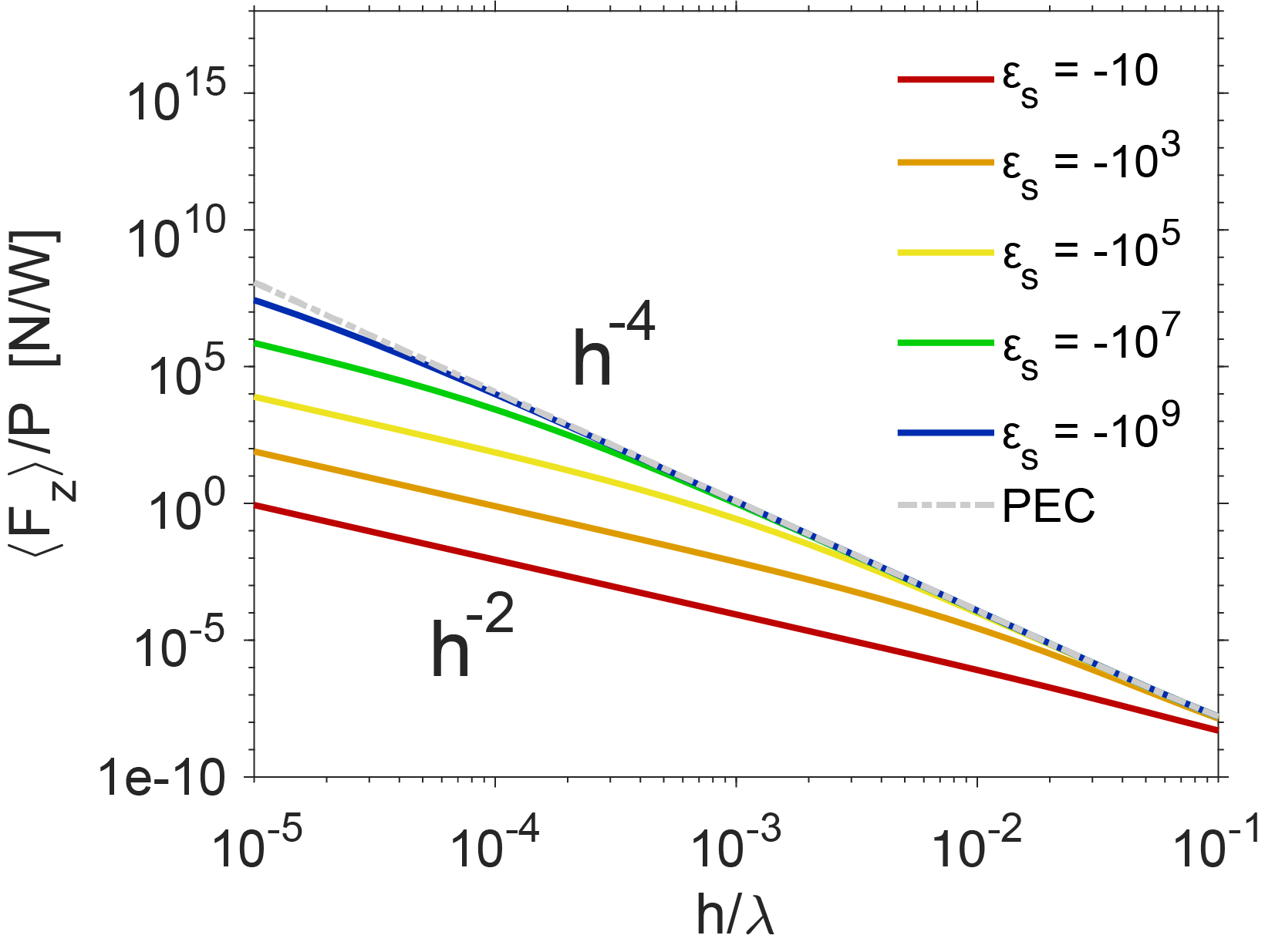
Figure S1: The height dependence of the normalized vertical force on a point VMD near substrates of varying permittivities. For large negative $\varepsilon_{s}$, the dipole is repelled as if it was a PEC substrate, until it reaches a height comparable to the skin depth, at which point the PEC model ($r_{s}=-1$) breaks down, and the quasistatic model becomes dominant and the height dependence switches from $h^{-4}$ to $h^{-2}$.

When conducting these calculations for various surfaces and extending the domain of $h$ down to extremely small distances, as is shown in Fig. S1, we see that only surfaces with a large negative $\varepsilon_{s}$ exhibit the $h^{-4}$ dependence of the PEC case and this gradually transitions towards the $h^{-2}$ dependence of Eq. (3) of the main text. Prior works that employ image theory to explain levitation Rodríguez-Fortuño et al. (2014) show a constant $h$ dependence in the quasistatic regime. It is therefore striking that we observe a transition in this case and it is an unexpected consequence of the higher order terms of $r_{s}$ altering the nature of the interaction.

I.4 Force on a rotated magnetic dipole

The theoretical analysis in the main text was restricted to the case of the exact VMD. This configuration was convenient because the VMD lacks any $p$-polarized scattering and the repulsive force is due to the $s$-polarized reflection. Since an experimental realization, with its corresponding limitations, may not achieve a perfectly vertical orientation, it is helpful to gauge the robustness of this $\mathfrak{Re}\{\varepsilon_{\text{s}}\}<1$ repulsion under dipole rotations.

Fig. S2a shows that rotating the dipole by small angles has no appreciable effect on the nature of the force. As the angle increases towards a HMD, a new attractive region appears near $\mathfrak{Re}\{\varepsilon_{\text{s}}\}=-1$ owing to the $p$-polarized surface plasmon resonance of the material. This signifies a competition between the attractive $p$ and repulsive $s$-polarized responses that depends strongly on $\mathfrak{Re}\{\varepsilon_{\text{s}}\}$. The HMD has the strongest $p$-polarization scattering of any magnetic dipole orientation and so for an experimental realization, this represents the worst case scenario for observing this effect. However Fig. S2d clearly shows that, even in that worst case, given $\mathfrak{Re}\{\varepsilon_{\text{s}}\}\lessapprox-5$, there exists a $h$ near the surface that will experience a repulsion. Given that most common metals fulfill this requirement, we therefore claim that the magnetic dipole repulsion is robust to significant rotation, assuming an appropriate surface material. The repulsion of the HMD is explained by means of image theory in Section I.2.

We note that extending this study to elliptical dipoles does not yield any new physics because the vertical force is invariant to the phases of the dipole moments, as can be seen from Eq. (S4). Diagonal and elliptical dipoles experience the same vertical forces and are merely linear combinations of the VMD and HMD.

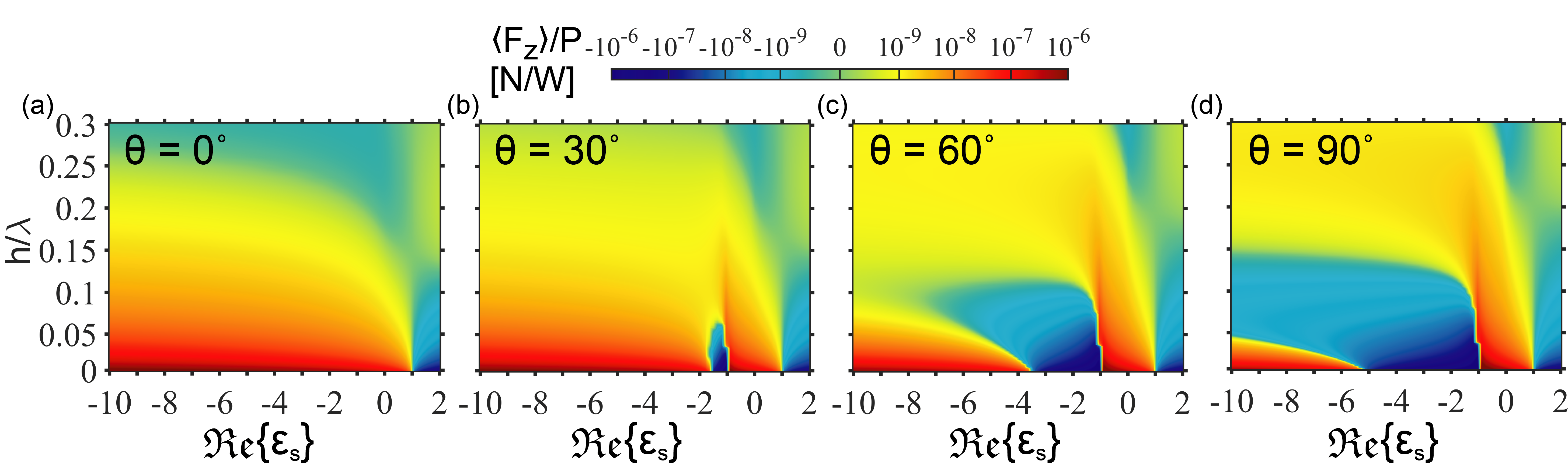
Figure S2: (a)-(d) As the VMD is rotated by the angle $\theta$, the time-averaged $\mathfrak{Re}\{\varepsilon_{\text{s}}\}<1$ repulsion is partially disrupted by a new attractive region. The attraction is driven by the $p$-polarized backscattering of the dipole and in the extreme case of the horizontal dipole, the repulsion remains dominant when $\mathfrak{Re}\{\varepsilon_{\text{s}}\}\lessapprox-5$ and $h$ is small enough. Note that the repulsion behavior is only disrupted for relatively large values of $\theta$ and so an approximately vertical dipole will experience the same force as the ideal case.

II Maxwell stress tensor calculations

The Maxwell stress tensor $\overset{\leftrightarrow}{\mathbf{T}}$ is a widely used technique in optics for determining the optical force on any body. The second rank tensor is derived from the flow of electromagnetic momentum through an arbitrary surface and is related to the time-averaged optical force by the following surface integral Novotny and Hecht (2006)

$$\langle\mathbf{F}\rangle=\int_{\mathcal{S}}\langle\overset{\leftrightarrow}{\mathbf{T}}\rangle\cdot\textbf{\^{n}}\,d\mathcal{S}$$ (S12)

where $\mathbf{F}$ is the force acting on a body and n̂ is the normal vector perpendicular to and out of any arbitrary closed surface $\mathcal{S}$ enclosing the body. The angular bracket notation around a single variable indicates a time averaging. $\langle\overset{\leftrightarrow}{\mathbf{T}}\rangle$ is defined as Novotny and Hecht (2006)

$$\langle\overset{\leftrightarrow}{\mathbf{T}}\rangle=\frac{1}{2}\mathbb{R}\bigg{\{}\varepsilon\mathbf{E}\otimes\mathbf{E}^{*}+\mu\mathbf{H}\otimes\mathbf{H}^{*}-\frac{1}{2}\big{(}\varepsilon|\mathbf{E}|^{2}+\mu|\mathbf{H}|^{2}\big{)}\overset{\leftrightarrow}{\mathbf{I}}\bigg{\}}$$ (S13)

where $\mathbf{E}$ and $\mathbf{H}$ are the total electric and magnetic fields, $\otimes$ denotes the outer product of two vectors, asterisks represent complex conjugations, $\overset{\leftrightarrow}{\mathbf{I}}$ is the identity matrix and $\varepsilon$ and $\mu$ are the permittivity and permeability of the medium, respectively.

In Fig. 1d of the main text, the electromagnetic fields were calculated analytically from Green’s theorem for a dipole over a surface Novotny and Hecht (2006), shown in Eq. I.1. For the core-shell system considered later in the main text, $\mathbf{E}$ and $\mathbf{H}$ were calculated in the time-domain with the commercial simulation software CST Microwave Studio. The force calculations of Fig. 2b were conducted in much the same way as Ref. Rodríguez-Fortuño et al. (2015). That is, the particle is illuminated with a plane wave and the total fields are calculated. The simulation is then repeated with the same mesh profile but without the particle. The fields from the latter simulation are then subtracted from the total fields to produce the scattered fields of the particle only, without the illumination. This allows us to isolate the the particle’s backscattering force from the radiation pressure of the illumination and compare directly with the general dipole theory, $F_{z}^{\text{th}}$.

We provide below in Fig. S3 the force calculated from the total fields, which includes the incident plane wave. This total force $F_{z}^{\text{tot}}$ corresponds to that what would be observed in an experiment. We note that the repulsion is still strongest around the magnetic resonance at 1.3 $\mu$m, and that this data highlights how strong the backscattering force is. The isolation of the backscattering force was presented in Fig. 2 of the main text because it allowed for a direct comparison with the general backscattering dipole force theory. The stress tensor calculations included varying the integration cube sizes to check for convergence.

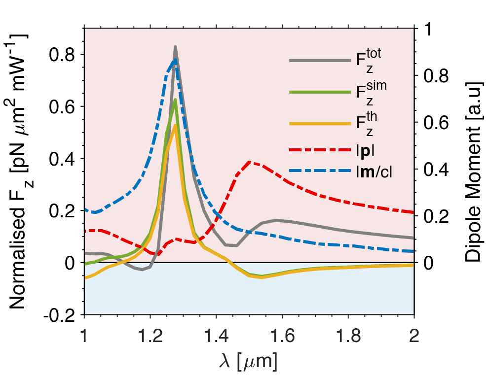
Figure S3: Wavelength dependence of $F_{z}^{\text{tot}}$, calculated from the total fields (including the plane wave), plotted alongside the retrieved dipole moments and backscattering force results from Fig. 2 in the main text.

III Dipole retrieval from a source near a surface

There are many methods for determining the induced electric and magnetic dipole resonances of an illuminated structure. Mie theory Bohren and Huffman (1998) is an exact solution for this problem if spherical symmetry is conserved but the presence of the surface in our current problem breaks this symmetry. Some methods also lack the ability to determine the orientation of the induced dipoles or the relative phase between their components. Rather than working with a weak assumption that the surface effects were negligible, we opted for our own method based on the decomposition of the scattered far fields into orthogonal basis functions. This method is valid for any system which can be described exactly with the angular representation and can be easily extended to higher order multipoles Vázquez-Lozano et al. (2019).

III.1 Decomposition of radiation pattern into orthogonal basis functions

We look to expand the numerically calculated radiation pattern $E_{\text{pattern}}$ in such a way that the complex Cartesian dipole moments are weighting coefficients

$$E_{\text{pattern}}=\,p_{x}\,\hat{E}_{p_{x}}+p_{y}\,\hat{E}_{p_{y}}+p_{z}\,\hat{E}_{p_{z}}+\frac{m_{x}}{c}\,\hat{E}_{m_{x}}+\frac{m_{y}}{c}\,\hat{E}_{m_{y}}+\frac{m_{z}}{c}\,\hat{E}_{m_{z}}.$$ (S14)

where $\hat{E}_{i}$ is a basis function corresponding to the radiation pattern of the $i^{\text{th}}$ dipole moment. For the purpose of our mathematical calculation, we take $p_{i}$ and $m_{i}$ to be dimensionless. However, these parameters gain units by comparing them with the dipole moments used to create the basis functions $\hat{E}$, which have units.

The retrieval method is reliant on a single condition; the basis functions must be orthogonal to each other. The far-field radiation diagrams for different multipoles would be exactly orthogonal in the case when the source was in free space, because they correspond to orthogonal vector spherical harmonics. However, we found out that when accounting for the surface reflection, the far-field radiation of the multipoles above the surface are no longer orthogonal to each other. Therefore, we had to apply an orthogonalization procedure enforced in Section III.3. Using this orthogonal basis,

$$E_{\text{pattern}}=\sum_{i=1}^{6}a_{i}\,\hat{E}_{i}$$ (S15)

where the coefficients $a_{i}=\langle\hat{E},\hat{E}_{i}\rangle/\langle\hat{E}_{i},\hat{E}_{i}\rangle$ and the angular bracket notation around two variables corresponds to their overlap integral, defined as $\langle E_{1},E_{2}\rangle=\iint\mathbf{E}_{1}\cdot\mathbf{E}_{2}^{*}\,d\Omega$, where $\Omega$ is the solid angle and the integration is conducted over the top hemisphere (i.e. far field radiation over the surface). A transformation is then performed to move from the orthogonalized basis to the basis of dipole moment of Eq. (S14).

III.2 Relating the angular spectrum representation to the far-field pattern

To obtain the radiation diagrams of the unit dipoles above a surface, we will rely on the angular spectrum representation of the scattered fields of a dipole near a surface, which are known analytically via Green’s function method for a dipole above a surface. These angular spectra can then be converted into the far-field distance-independent pattern $\mathbf{E}_{\text{pattern}}(\theta,\phi)$. That is to say, the exact fields of a dipole in Fourier space can be converted into a distance-independent radiation pattern which commercial software can readily compute for any physical scenario. $\mathbf{E}_{\text{pattern}}$ is related to the far fields $\mathbf{E}_{\text{far}}$ by

$$\mathbf{E}_{\text{far}}(\mathbf{r})=\mathbf{E}_{\text{pattern}}(\theta,\phi)\,\frac{e^{i\,k_{0}\,r}}{r}.$$ (S16)

We write the real-space fields here in spherical coordinates to align with the convention in radiation patterns, where $\mathbf{r}=(r,\theta,\phi)$ is the general position vector in spherical coordinates. The angular representation derives from the Weyl identity

$$\frac{e^{i\,k_{0}\,r}}{r}=\iint\frac{i\,k_{0}}{2\pi}e^{i\,\mathbf{k}\cdot\mathbf{r}}d\Omega.$$ (S17)

The definition of the angular representation itself is

$$\mathbf{E}(\mathbf{r})=\iint k_{0}\,k_{z}\,\mathbf{E}(k_{x},k_{y};0)e^{i\,\mathbf{k}\cdot\mathbf{r}}d\Omega.$$ (S18)

Note that this definition differs to that of Eq. (I.1) where the integrals are in terms of $dk_{x}$ and $dk_{y}$. Here, we have transformed the integrals in (S17) and (S18) into the solid angle $\Omega$ of a sphere.

Our aim is to find a clear relation between $\mathbf{E}_{\text{pattern}}(\theta,\phi)$ and $\mathbf{E}(k_{x},k_{y};0)$. To do this, we can find the relation for a simple example. In the far field, the far field pattern of a VED is $\mathbf{E}_{\text{far}}\propto\text{sin}(\theta)\frac{e^{i\,k_{0}\,r}}{r}$ and therefore $\mathbf{E}_{\text{pattern}}\propto\text{sin}(\theta)$. Substituting these relations into Eq. (S17) leads to

$$\text{sin}(\theta)\frac{e^{i\,k_{0}\,r}}{r}=\iint\frac{k_{t}}{k_{0}}\frac{i\,k_{0}}{2\pi}e^{i\,\mathbf{k}\cdot\mathbf{r}}d\Omega=\iint\frac{i\,k_{t}}{2\pi}e^{i\,\mathbf{k}\cdot\mathbf{r}}d\Omega.$$ (S19)

Comparing (S19) with (S18) leads us to the desired transformation in a generalized form which will be true in general for any point source

$$\mathbf{E}_{\text{pattern}}(\theta,\phi)=-2\,\pi\,i\,k_{z}\,\mathbf{E}(k_{x},k_{y};0).$$ (S20)

III.3 Orthogonal basis functions in angular representation

The angular representation of the exact scattered fields of an electric or magnetic dipole, at $z=h$, with a reflecting surface at $z=0$ are known Picardi et al. (2017),

$$\mathbf{E}(k_{x},k_{y};0) =\begin{pmatrix}E_{k}\\ E_{s}\\ E_{p}\end{pmatrix}\xLongrightarrow{\text{far-field}}\begin{pmatrix}E_{r}\\ E_{\phi}\\ E_{\theta}\end{pmatrix}=$$

$$E^{\text{self}}_{\phi}(k_{x}, k_{y};0)=\frac{i\,k_{0}^{2}}{8\pi^{2}\varepsilon_{0}k_{z}}\,\Big{(}\hat{\mathbf{e}}_{s}\cdot\mathbf{p}-\hat{\mathbf{e}}_{p}^{+}\cdot\frac{\mathbf{m}}{c}\Big{)}\,e^{-ik_{z}h}$$

$$E^{\text{ref}}_{\phi}(k_{x}, k_{y};0)=\frac{i\,k_{0}^{2}}{8\pi^{2}\varepsilon_{0}k_{z}}\,r_{s}\,\Big{(}\hat{\mathbf{e}}_{s}\cdot\mathbf{p}-\hat{\mathbf{e}}_{p}^{-}\cdot\frac{\mathbf{m}}{c}\Big{)}\,e^{ik_{z}h}.$$

$$E^{\text{self}}_{\theta}(k_{x}, k_{y};0)=\frac{i\,k_{0}^{2}}{8\pi^{2}\varepsilon_{0}k_{z}}\,\Big{(}\hat{\mathbf{e}}_{p}^{+}\cdot\mathbf{p}+\hat{\mathbf{e}}_{s}\cdot\frac{\mathbf{m}}{c}\Big{)}\,e^{-ik_{z}h}$$

$$E^{\text{ref}}_{\theta}(k_{x}, k_{y};0)=\frac{i\,k_{0}^{2}}{8\pi^{2}\varepsilon_{0}k_{z}}\,r_{p}\,\Big{(}\hat{\mathbf{e}}_{p}^{-}\cdot\mathbf{p}+\hat{\mathbf{e}}_{s}\cdot\frac{\mathbf{m}}{c}\Big{)}\,e^{ik_{z}h}$$

When only considering the electric and magnetic dipole, one can form six basis functions by simply setting all but one component of the electromagnetic dipole to zero and substituting (III.3) into (S20). Thus the first basis function could be formed from $(p_{x},p_{y},p_{z},m_{x},m_{y},m_{z})\rightarrow{}(1,0,0,0,0,0)$.

Though we have now formed six basis functions, they do not yet necessarily form an orthogonal set. To meet the orthogonalization condition outlined in Subsection III.1, we can apply the Gram-Schmidt procedure

$$\mathbf{u}_{1} =\mathbf{v}_{1}$$

$$\mathbf{u}_{k}=\mathbf{v}_{k}- \sum_{j=1}^{k-1}\frac{\langle\mathbf{v}_{k},\mathbf{u}_{j}\rangle}{\langle\mathbf{u}_{j},\mathbf{u}_{j}\rangle}\mathbf{u}_{j},$$ (S22)

where $\mathbf{u}$ is a general basis vector from a non-orthogonal set which is orthogonalized to form $\mathbf{v}$ which forms an orthogonal set of vectors. This enables us to obtain an orthogonal basis (as in S15) from the original dipolar basis (S14). The new set of orthogonal radiation pattern basis functions become combinations of dipole moments which are linearly independent from one another.