, , and t1Corresponding author. Email: liuruiq@iu.edu m1Department of Mathematical Sciences, Indiana University - Purdue University Indianapolis , IN 46202, USA. m2Department of Mathematical Sciences, New Jersey Institute of Technology, NJ 07102, USA. t2Sponsored by NSF DMS-1764280 and NSF DMS-1821157

This version

Statistical Inference on Partially Linear Panel Model under Unobserved Linearity

Abstract

A new statistical procedure, based on a modified spline basis, is proposed to identify the linear components in the panel data model with fixed effects. Under some mild assumptions, the proposed procedure is shown to consistently estimate the underlying regression function, correctly select the linear components, and effectively conduct the statistical inference. When compared to existing methods for detection of linearity in the panel model, our approach is demonstrated to be theoretically justified as well as practically convenient. We provide a computational algorithm that implements the proposed procedure along with a path-based solution method for linearity detection, which avoids the burden of selecting the tuning parameter for the penalty term. Monte Carlo simulations are conducted to examine the finite sample performance of our proposed procedure with detailed findings that confirm our theoretical results in the paper. Applications to Aggregate Production and Environmental Kuznets Curve data also illustrate the necessity for detecting linearity in the partially linear panel model.

Keywords: Semiparametric model, Panel data, Fixed effects, Linearity detection, Penalized estimation, Partially linear regression

Keywords: C01, C14, C33

1 Introduction

Panel models have attracted much attention from economists and econometricians, especially for their flexibility in modeling homogeneity while preserving individual-level heterogeneity. With the rapid increase in availability of panel data in the past two decades or so, panel models in both parametric and nonparametric frameworks have been well studied in the literature; see Ruckstuhl et al., (2000), Henderson et al., (2008), Freyberger, (2017), Su and Zhang, (2015), Hsiao and Tahmiscioglu, (1997), Lee and Robinson, (2015), Hsiao and Tahmiscioglu, (2008), Hsiao and Tahmiscioglu, (1997), and Hsiao, (2014). Still, either framework, parametric or nonparametric, is not fully satisfactory in modeling panel data, as each has its own advantages and drawbacks. In light of its simplicity and interpretability, the parametric model becomes a prominent tool for panel data analysis; see Baltagi and Griffin, (1983), Dahlberg and Johansson, (2000), Koop and Tobias, (2004), Solow, (1957), Griliches, (1964), Bloom et al., (2004). However, when compared to the nonparametric model, it appears to be more sensitive to model misspecification, which is often the case in empirical applications. Based on fewer model assumptions, the nonparametric model can lead to a more robust estimator, especially when dealing with relatively large panel data sets. On the other hand, with a larger dimension of input data, a purely nonparametric model is usually not preferred in empirical applications due to the infamous “Curse of Dimensionality” issue and the poor model interpretability. To address these noted drawbacks and make the best use of the apparent advantages, the partially linear panel model strikes a balance between parametric and nonparametric frameworks. For instance, Henderson et al., (2008) studied both nonparametric and partially linear panel models with fixed effects and proposed a kernel estimator with a corresponding linearity specification test. Combining the works by Henderson et al., (2008) and Mammen et al., (2009), Li and Liang, (2015) proposed a two-step estimator in partially linear panel; Baltagi and Li, (2002) considered the problem of estimating a partially linear fixed effects panel model with possible endogeneity and lagged dependent variables in the linear part; Su and Zhang, (2016) proposed estimation and specification testing procedures for partially linear dynamic panel model with fixed effects, with either exogenous or endogenous variables or both in the linear part and the lagged dependent variables, together with some other exogenous variables entering nonparametrically in the model. Following Su and Zhang, (2016), Su and Zhang, (2015) extended their work to the panel model with interactive fixed effects.

In practice, however, when considering the partially linear model, the researchers need to consider the following two questions: (a) which variables should be included in the model? (b) what is the functional form of each variable? Various statistical variable selection techniques, such as Liang and Li, (2009), Xue, (2009), Huang et al., (2010), are available to address the first question. Nevertheless, in the context of economic modeling, one would prefer to select the dependent variables also by economic theory, as relying on purely statistical variable selection procedures may fit a model which is lacking in its economic justification and interpretability, see Bartolucci et al., (2018), Baxa et al., (2015), Kilian and Park, (2009), Deaton, (2008). Even though the economic theory can explain which variables should be included in the model, it fails to specify the functional forms of the variables. Therefore, the second question is of more practical importance than the first one. Misspecification of the functional forms of the regressors can either (a) result in inconsistent estimation if fitting nonlinear functions by linear forms, (b) or reduce the model interpretability and estimation efficiency if the linear functions are estimated nonparametrically. Thus, correct specification of the linear components, if any, is essential to improve estimation and model explainability. However, to the best of our knowledge, all the linearity detection methods advocated in the literature on partially linear panel model, are all based on specification tests; see Henderson et al., (2008), Su and Zhang, (2016) and Su and Zhang, (2015). One primary drawback to this approach is that the test statistics is often difficult to construct and may be deficient in its power when the number of dependent variables is large, which may lead to incorrect model specification. Under cross-sectional data settings, Zhang et al., (2011) propose a smoothing-spline-type estimator which is able to estimate the underlying regression function and discover the linear regressors simultaneously. However, how to conduct valid statistical inference using the approach in Zhang et al., (2011) is still unknown.

The main purpose of this paper is to propose a unified statistical procedure capable of simultaneously estimating underlying regression function, detecting linear components, and conducting inference in the partially linear panel. This paper is organized as follows. In Section 2, we mathematically formulate the linearity detection problem in the partially linear panel model. In Section 3, we propose a penalized estimator for linearity detection, and provide the corresponding computational algorithm. The asymptotic properties of the proposed estimator and the corresponding linearity detection procedure are established in Section 4 for both short and large panels. In Section 5, we discuss how to determine the tuning parameters involved in the proposed procedure. Section 6 carries out a set of Monte Carlo simulations to investigate the finite sample performance of our proposed method. Applications to two real-world datasets are provided in Section 7. Technical details and proofs of the main theorems and auxiliary results are deferred in the Appendix. Throughout this paper, we use the following notation.

Notation: Define $\otimes$ as the tensor product operator. For positive real number $m$, let $\left\lfloor m\right\rfloor$ be the largest integer that is strictly less than $m$ and $\lceil m\rceil=\left\lfloor m\right\rfloor+1$. Denote $(x)_{+}=\max(x,0)$ for $x\in\mathbb{R}$.

2 Partially Linear Panel Model with Unknown Structure

Suppose that the observations $\{(Y_{it},\mathbf{Z}_{it}),i=1,\ldots,N,t=1,\ldots,T\}$ are generated from the following model

$$Y_{it}=f_{0}(\mathbf{Z}_{it})+\alpha_{i}^{0}+\epsilon_{it},$$ (2.1)

where $Y_{it}$ is the response variable, $\mathbf{Z}_{it}=(Z_{it1},Z_{it2},\ldots,Z_{itp})^{\top}\in\mathcal{Z}\mathrel{\mathop{\mathchar 58\relax}}=[0,1]^{p}$ are explanatory variables, both observed for individual $i$ at time period $t$, $\alpha_{i}^{0}\in\mathbb{R}$ are unobservable individual-level fixed effects, $\epsilon_{it}\in\mathbb{R}$ is unobservable errors. Assume that the unknown regression function $f_{0}\mathrel{\mathop{\mathchar 58\relax}}\mathcal{Z}\to\mathbb{R}$ has the following semiparametric expression:

$$f_{0}(\mathbf{z})=\sum_{j\in J_{\textrm{lin}}}f_{j,0}(z_{j})+\sum_{j\in J_{\textrm{lin}}^{c}}f_{j,0}(z_{j}),\mathbf{z}=(z_{1},\ldots,z_{p})\in\mathcal{Z},$$

where $J_{\textrm{lin}}$ is a (unknown) subset of $\{1,\ldots,p\}$ and $J_{\textrm{lin}}^{c}$ denotes its complement, $f_{j,0}$ for $j\in J_{\textrm{lin}}$ are linear functions and $f_{j,0}$ for $j\in J_{\textrm{lin}}^{c}$ are nonlinear. Our aim is to identify $J_{\textrm{lin}}$ as well as to conduct statistical inference about $f_{0}$ based on the observations. Without loss of generality, we may assume that $J_{\textrm{lin}}=\{1,2,\ldots,d\}$ for some nonnegative integer $d\leq p$, therefore, $f_{1,0},\ldots,f_{d,0}$ are linear and $f_{d+1,0},\ldots,f_{p,0}$ are nonlinear. For convenience, define $\{1,\ldots,d\}$ as the empty set when $d=0$.

3 Penalized Estimation

In this section, we propose a penalized sieve estimator based on a modified spline basis, which can consistently estimate the underlying regression function $f_{0}$, effectively identify the linear components, and validly conduct statistical inference.

3.1 Centralized Spline

To estimate $f_{0}=\sum_{j=1}^{p}f_{j,0}$, we follow the idea of sieve estimation, i.e., estimating each $f_{j,0}$ by a linear combination of basis functions. The common basis function used in literature includes B-spline basis, wavelet basis, etc. (see Chen,, 2007 for an excellent review of sieve basis). However, for linearity detection purpose, the existing bases are not adequate. Thus, we will propose a modified spline space and the corresponding basis to address this issue. Given $M+1$ strictly increasing knots $\mathbf{t}_{M}=\{t_{0},t_{1},\ldots,t_{M}\}$ with $t_{0}=0,t_{M}=1$ and integer $r\geq 1$, define $r$-th degree Centralized Spline Space

$$\textrm{CSpl}(r,\mathbf{t}_{M})=\bigg{\{}\sum_{k=1}^{r}c_{k}\psi_{k}(z)+\sum_{k=1}^{M-1}\widetilde{c}_{k}\widetilde{\psi}_{k}(z)\mathrel{\mathop{\mathchar 58\relax}}z\in[0,1],c_{k},\widetilde{c}_{k}\in\mathbb{R}\bigg{\}},$$

with

$$\psi_{1}(z) =z-\frac{1}{2},\;\;\psi_{k}(z)=\bigg{(}z^{k}-\frac{1}{k+1}\bigg{)}-\frac{6k}{(k+1)(k+2)}\bigg{(}z-\frac{1}{2}\bigg{)},\textrm{ for }k=2,\ldots,r,$$

$$\widetilde{\psi}_{k}(z) =\bigg{(}(z-t_{k})^{r}_{+}-\frac{1}{r+1}(1-t_{k})^{r+1}\bigg{)}-\bigg{\{}\frac{6(1-t_{k})^{r+1}}{(r+1)}-\frac{12(1-t_{k})^{r+2}}{(r+1)(r+2)}\bigg{\}}\bigg{(}z-\frac{1}{2}\bigg{)},$$

$$\textrm{ for }k=1,\ldots,M-1,$$

being the corresponding Centralized Spline Basis. Expressed by centralized spline basis, any function in centralized spline space can be decomposed two orthogonal parts. To be more specific, for any $f=\sum_{k=1}^{r}c_{k}\psi_{k}+\sum_{k=1}^{M-1}\widetilde{c}_{k}\widetilde{\psi}_{k}\in\textrm{CSpl}(r,\mathbf{t}_{M})$, we decompose $f=f_{-}+f_{\sim}$, with

$$f_{-}(z)=c_{1}\psi_{1}(z)=c_{1}(z-1/2)\;\;\textrm{ and }\;\;f_{\sim}(z)=\sum_{k=2}^{r}c_{k}\psi_{k}(z)+\sum_{k=1}^{M-1}\widetilde{c}_{k}\widetilde{\psi}_{k}(z),$$ (3.1)

which are corresponding to the linear and nonlinear components. It can be verified that

$$\int_{0}^{1}f_{-}(z)f_{\sim}(z)dz=0.$$ (3.2)

Remark 1.

The centralized spline basis essentially is an orthogonal version of the polynomial spline basis $\{z,z^{2},\ldots,z^{r},(z-t_{1})^{r}_{+},\ldots,(z-t_{M-1})^{r}_{+}\}$. However, compared to the classical polynomial splines or B-splines, centralized spline basis is able to effectively separate the linear part from the nonlinear component due to (3.2). Even though, all the bases generate similar function spaces and the difference is only up to a constant.

3.2 Penalized Estimator

We begin by introduing the following function spaces

$$\mathcal{H}=\bigg{\{}f\mathrel{\mathop{\mathchar 58\relax}}\mathcal{Z}\to\mathbb{R}\;|\;\int_{\mathcal{Z}}f^{2}(\mathbf{z})d\mathbf{z}<\infty\bigg{\}}\textrm{,\;\;\; }\mathcal{H}_{0}=\bigg{\{}f\in H\;|\;\int_{\mathcal{Z}}f(\mathbf{z})d\mathbf{z}=0\bigg{\}},$$

and

$$\Theta_{NT}=\bigg{\{}f(\mathbf{z})=\sum_{j=1}^{p}f_{j}(z_{j})\;|\;f_{j}\in\Theta_{NT,j},\textrm{ for }j\in[p]\bigg{\}},$$ (3.3)

where $\Theta_{NT,j}=\textrm{CSpl}(r_{j},\mathbf{t}_{j,M_{j}})$ for some integers $M_{j},r_{j}\geq 1$ and knots $\mathbf{t}_{j,M_{j}}=(t_{j,0},\ldots,t_{j,M_{j}})$ with $t_{j,0}=0,t_{j,M_{j}}=1$ for $j\in[p]$. Clearly, $\Theta_{NT}$ is a linear subspace of $\mathcal{H}_{0}$ and in the following it will be the sieve space to estimate the underlying regression function $f_{0}$. Moreover, for $g,f\in\mathcal{H}$, we introduce the following notation when the corresponding values exist,

$$\zeta_{i}(g,f) =\frac{1}{T}\sum_{t=1}^{T}\bigg{(}g(\mathbf{Z}_{it})-\frac{1}{T}\sum_{s=1}^{T}g(\mathbf{Z}_{is})\bigg{)}\bigg{(}f(\mathbf{Z}_{it})-\frac{1}{T}\sum_{s=1}^{T}f(\mathbf{Z}_{is})\bigg{)},$$

$$\langle g,f\rangle_{NT} =\frac{1}{N}\sum_{i=1}^{N}\zeta_{i}(g,f),\;\;\langle g,f\rangle=\mathbb{E}(\langle g,f\rangle_{NT}),\;\;\|g\|_{NT}^{2}=\langle g,g\rangle_{NT},\;\;\|g\|^{2}=\langle g,g\rangle.$$

We can show that under mild assumptions, $\langle\cdot,\cdot\rangle$ is a valid inner product on $\Theta_{NT}$ (see Lemma A.1 and Lemma A.12 for details). By above notation, we define a penalized objective function on $\Theta_{NT}$ as follows. For $f(\mathbf{z})=\sum_{j=1}^{p}f_{j}(z_{j})\in\Theta_{NT}$ with $f_{j}\in\Theta_{NT,j}$, let

$$l_{NT}(f)=\frac{1}{NT}\sum_{i=1}^{N}\sum_{t=1}^{T}\bigg{[}Y_{it}-f(\mathbf{Z}_{it})-\frac{1}{T}\sum_{s=1}^{T}\bigg{(}Y_{is}-f(\mathbf{Z}_{is})\bigg{)}\bigg{]}^{2}+\sum_{j=1}^{p}p_{\lambda_{NT}}\bigg{(}\|f_{j,\sim}\|_{NT}\bigg{)},$$ (3.4)

where $f_{j,\sim}$ is the nonlinear component of $f_{j}$ as defined in (3.1), and $p_{\lambda_{NT}}$ is a given penalty function with tuning parameter $\lambda_{NT}$. The penalized estimator is defined as the minimizer of (3.4), namely,

$$\widehat{f}=\mathop{\mathrm{argmin}}_{f\in\Theta_{NT}}l_{NT}(f).$$ (3.5)

There are several possible choices for the functional form of the penalty term $p_{\lambda_{NT}}$. To name a few, Ridge penalty for $p_{\lambda_{NT}}(z)=\lambda_{NT}z^{2}$, Lasso penalty (Tibshirani,, 1996) for $p_{\lambda_{NT}}(z)=\lambda_{NT}|z|$, and Smoothly Clipped Absolute Deviation (SCAD) penalty (Fan and Li,, 2001) for $p_{\lambda_{NT}}$ with first order derivative

$$p^{\prime}_{\lambda_{NT}}(z)=\lambda_{NT}I(z\leq\lambda_{NT})+\frac{(\kappa\lambda_{NT}-z)_{+}}{\kappa-1}I(z>\lambda_{NT}),$$ (3.6)

where $\kappa>2$ is some predetermined constant. In general, with larger $\lambda_{NT}$, the penalty function $p_{\lambda_{NT}}$ will be larger and thus (3.4) will tend to shrink the nonlinear components $f_{j,\sim}$’s. When compared to other penalties, the solution via SCAD penalty simultaneously enjoys three desirable properties, i.e., unbiasedness, sparsity, and continuity, see Fan and Li, (2001) for a detailed discussion. Therefore, throughout this paper, we will consider $p_{\lambda_{NT}}$ as SCAD penalty, and extension to other types of penalties are left as future work.

3.3 Computational Algorithm

In this section we propose a local quadratic approximation algorithm to solve optimization problem in (3.5). For each $j=1,\ldots,p$, let $\psi_{j,1},\psi_{j,2},\ldots,\psi_{j,r_{j}},\widetilde{\psi}_{j,1},\ldots,\widetilde{\psi}_{j,M_{j}-1}$ be the centralized spline basis and for any $f_{j}\in\Theta_{NT,j}$, it follows that $f_{j}(z)=f_{j,-}(z)+f_{j,\sim}(z)$, with $f_{j,-}(z)=v_{j}\psi_{j,1}(z)\textrm{ and }f_{j,\sim}=u_{j}^{\top}\mathbf{\Psi}_{j,\sim}(z),$ for some $v_{j}\in\mathbb{R}$, $u_{j}\in\mathbb{R}^{M_{j}+r_{j}-2}$, and all $z\in[0,1]$. Here $\mathbf{\Psi}_{j,\sim}(z)=(\psi_{j,2}(z),\ldots,\psi_{j,r_{j}}(z),\widetilde{\psi}_{j,1}(z),\ldots,\widetilde{\psi}_{j,M_{j}-1}(z))^{\top}$ is a $(M_{j}+r_{j}-2)$-dimensional vector of functions. Furthermore, for each $j\in[p]$, we define vectors

$$\mathbf{B}_{j,\sim} =(\mathbf{\Psi}_{j,\sim}(Z_{11j}),\mathbf{\Psi}_{j,\sim}(Z_{12j}),\ldots,\mathbf{\Psi}_{j,\sim}(Z_{itj}),\ldots,\mathbf{\Psi}_{j,\sim}(Z_{NTj}))^{\top}\in\mathbb{R}^{NT\times(M_{j}+r-2)},$$

$$v =(v_{1},\ldots,v_{p})^{\top}\in\mathbb{R}^{p},\;\mathbf{Y}=(Y_{11},Y_{12},\ldots,Y_{it},\ldots,Y_{NT})^{\top}\in\mathbb{R}^{NT}$$

and matrices

$$\mathbf{B}_{-} =\begin{pmatrix}\psi_{1,1}(Z_{111})&\psi_{2,1}(Z_{112})&\ldots&\psi_{p,1}(Z_{11p})\\ \psi_{1,1}(Z_{121})&\psi_{2,1}(Z_{122})&\ldots&\psi_{p,1}(Z_{12p})\\ \vdots&\vdots&\vdots&\vdots\\ \psi_{1,1}(Z_{it1})&\psi_{2,1}(Z_{it2})&\ldots&\psi_{p,1}(Z_{itp})\\ \vdots&\vdots&\vdots&\vdots\\ \psi_{1,1}(Z_{NT1})&\psi_{2,1}(Z_{NT2})&\ldots&\psi_{p,1}(Z_{NTp})\\ \end{pmatrix}\in\mathbb{R}^{NT\times p},$$

$$H =I_{T}-\frac{1}{T}uu^{\top}\in\mathbb{R}^{T\times T},\;\textrm{ with }u=(1,1,\ldots,1)^{\top}\in\mathbb{R}^{T},\;\;M_{H}=I_{N}\otimes H\in\mathbb{R}^{NT\times NT}.$$

By using the above notation, it is not difficult to verify the following equalities,

$$\|f_{j,\sim}\|_{NT}^{2}=\frac{1}{NT}u_{j}^{\top}\mathbf{B}_{j,\sim}^{\top}M_{H}\mathbf{B}_{j,\sim}u_{j}$$

and

$$l_{NT}(f)=\frac{1}{NT}\bigg{(}\mathbf{Y}-\mathbf{B}_{-}v-\sum_{j=1}^{p}\mathbf{B}_{j,\sim}u_{j}\bigg{)}^{\top}M_{H}\bigg{(}\mathbf{Y}-\mathbf{B}_{-}v-\sum_{j=1}^{p}\mathbf{B}_{j,\sim}u_{j}\bigg{)}$$

$$+\sum_{j=1}^{p}p_{\lambda_{NT}}\bigg{(}\sqrt{\frac{1}{NT}u_{j}^{\top}\mathbf{B}_{j,\sim}^{\top}M_{H}\mathbf{B}_{j,\sim}u_{j}}\bigg{)}.$$ (3.7)

Therefore, the optimization problem in (3.5) is adapted to the optimization problem in (3.7), which is reduced to finding the corresponding minimizer $v$ and $u_{j}$’s. As in Fan and Li, (2001), we will also use quadratic functions to approximate the penalty terms in (3.7). Note that

$$\frac{\partial p_{\lambda}\bigg{(}\sqrt{\frac{1}{NT}u^{\top}\mathbf{B}_{j,\sim}^{\top}M_{H}\mathbf{B}_{j,\sim}u}\bigg{)}}{\partial u}=\frac{\sqrt{NT}p^{\prime}_{\lambda}\bigg{(}\sqrt{\frac{1}{NT}u^{\top}\mathbf{B}_{j,\sim}^{\top}M_{H}\mathbf{B}_{j,\sim}u}\bigg{)}\mathbf{B}_{j,\sim}^{\top}M_{H}\mathbf{B}_{j,\sim}u}{\sqrt{u^{\top}\mathbf{B}_{j,\sim}^{\top}M_{H}\mathbf{B}_{j,\sim}u}},$$

provided $u^{\top}\mathbf{B}_{j,\sim}^{\top}M_{H}\mathbf{B}_{j,\sim}u>0$. Therefore, if $u\approx u^{0}$, Taylor expansion leads to

$$p_{\lambda}\bigg{(}\sqrt{\frac{1}{NT}u^{\top}\mathbf{B}_{j,\sim}^{\top}M_{H}\mathbf{B}_{j,\sim}u}\bigg{)}$$

$$\approx p_{\lambda}\bigg{(}\sqrt{\frac{1}{NT}u^{0\top}\mathbf{B}_{j,\sim}^{\top}M_{H}\mathbf{B}_{j,\sim}u^{0}}\bigg{)}+D_{j}(u^{0})u^{\top}\mathbf{B}_{j,\sim}^{\top}M_{H}\mathbf{B}_{j,\sim}(u-u^{0})$$

$$\approx p_{\lambda}\bigg{(}\sqrt{\frac{1}{NT}u^{0\top}\mathbf{B}_{j,\sim}^{\top}M_{H}\mathbf{B}_{j,\sim}u^{0}}\bigg{)}+D_{j}(u^{0})\bigg{[}u^{\top}\mathbf{B}_{j,\sim}^{\top}M_{H}\mathbf{B}_{j,\sim}u-u^{0\top}\mathbf{B}_{j,\sim}^{\top}M_{H}\mathbf{B}_{j,\sim}u^{0}\bigg{]},$$

with $D_{j}(u^{0})=\sqrt{NT}p^{\prime}_{\lambda}\left(\sqrt{\frac{1}{NT}\smash[b]{u^{0\top}\mathbf{B}_{j,\sim}^{\top}M_{H}\mathbf{B}_{j,\sim}u^{0}}}\right)\left(u^{0\top}\mathbf{B}_{j,\sim}^{\top}M_{H}\mathbf{B}_{j,\sim}u^{0}\right)^{-1/2}$ and provided $D_{j}(u^{0})$ exists. As a consequence, if $u_{j}\approx u_{j}^{0}$ for all $j=1,\ldots,p$, (3.7) can be locally approximated, up to a constant, by

$$\frac{1}{NT}\bigg{(}\mathbf{Y}-\mathbf{B}_{-}v-\sum_{j=1}^{p}\mathbf{B}_{j,\sim}u_{j}\bigg{)}^{\top}M_{H}\bigg{(}\mathbf{Y}-\mathbf{B}_{-}v-\sum_{j=1}^{p}\mathbf{B}_{j,\sim}u_{j}\bigg{)}+\sum_{j=1}^{p}D_{j}(u^{0}_{j})u^{\top}_{j}\mathbf{B}_{j,\sim}^{\top}M_{H}\mathbf{B}_{j,\sim}u_{j}.$$

From above equation, we summarize the proposed algorithm below.

1. Choose initial values $(fv^{(0)},u_{1}^{(0)},\ldots,u_{p}^{(0)})$.

2. In the $s$-th iteration, solve following optimization problem:

   $$(v^{(s+1)},u_{1}^{(s+1)},\ldots,u_{p}^{(s+1)})= \operatorname*{argmin}_{v,u_{1},\ldots,u_{p}}\bigg{(}\mathbf{Y}-\mathbf{B}_{-}v-\sum_{j=1}^{p}\mathbf{B}_{j,\sim}u_{j}\bigg{)}^{\top}M_{H}\bigg{(}\mathbf{Y}-\mathbf{B}_{-}v-\sum_{j=1}^{p}\mathbf{B}_{j,\sim}u_{j}\bigg{)}$$

   $$+NT\sum_{j=1}^{p}D_{j}(u^{(s)}_{j})u^{\top}_{j}\mathbf{B}_{j,\sim}^{\top}M_{H}\mathbf{B}_{j,\sim}u_{j}.$$ (3.8)

3. Repeat (b) until the difference between $(v^{(s)},u_{1}^{(s)},\ldots,u_{p}^{(s)})$ and $(v^{(s+1)},u_{1}^{(s+1)},\ldots,u_{p}^{(s+1)})$ is small enough.

Remark 2.

It is worthwhile mentioning that the optimization problem in (3.8) is a ridge-type regression problem, which can significantly reduces the computatioal complexity. For convergence analysis of the proposed algorithm, we refer the readers to Xue, (2009) and Hunter and Li, (2005).

4 Asymptotic Theory

In this section we present several asymptotic results concerning our proposed procedure for both short panel (fixed $T$) and large panel (diverging $T$). However, before proceeding further, we remind the readers the Holder-smoothness notion of a function. An univariate function $f\mathrel{\mathop{\mathchar 58\relax}}[0,1]\to\mathbb{R}$ is said to be $m$-smooth, if $m=r+\delta$, for some $0<\delta\leq 1$ and integer $r$ such that $f$ is $r$-times continuously differentiable and $|f^{(r)}(u)-f^{(r)}(v)|\leq c|u-v|^{\delta}$ for some $c>0$ and all $u,v\in[0,1]$. Additionally, in the sequel, we use the following notation. We let $q_{i}(\mathbf{w})$ be the density function of $\mathbf{W}_{i}=(\mathbf{Z}_{i1},\ldots,\mathbf{Z}_{iT})$ and $\pi_{i}(\mathbf{z})$ be the density function of $\mathbf{Z}_{i1}$. For a function $g\mathrel{\mathop{\mathchar 58\relax}}[0,1]^{k}\to\mathbb{R}$, we define $\|g\|_{2}^{2}=\int g^{2}(\mathbf{u})d\mathbf{u}-[\int g(\mathbf{u})d\mathbf{u}]^{2}$ whenever the integrals exist. Finally we set $\mathbb{Z}=(\mathbf{W}_{1},\mathbf{W}_{2},\ldots,\mathbf{W}_{N})$ and $\bm{\epsilon}=(\epsilon_{11},\epsilon_{12},\ldots,\epsilon_{it},\ldots,\epsilon_{NT})^{\top}\in\mathbb{R}^{NT}$.

4.1 Consistency

The main results of this section show that the proposed penalized estimator is consistent in terms of both estimation and linearity detection. However, these results require some technical conditions, which are stated as follows.

Assumption A1.

1. $T$ is a fixed constant.

2. For some $a_{1}>1$ , it satisfies that $a_{1}^{-1}\leq q_{i}(\mathbf{w})\leq a_{1}$ for all $i=1,\ldots,N$ and all $\mathbf{w}\in[0,1]^{pT}$.

Assumption A2.

1. $T$ is diverging.

2. For some $a_{3}>1$ and $0\leq a_{4}<1$, it satisfies that $a_{3}^{-1}\leq\pi_{i}(\mathbf{z})\leq a_{3}$ for all $i=1,\ldots,N$ and all $\mathbf{z}\in\mathcal{Z}$. For each $i$, $\{\mathbf{Z}_{i1},\ldots,\mathbf{Z}_{iT}\}$ is a stationary alpha-mixing sequence with alpha mixing coefficient $\alpha_{[i]}(t)\leq a_{4}^{t}$ for all $t\geq 0$.

Assumption A3.

1. $\{\mathbf{W}_{i},i=1,\ldots,N\}$ are independent across $i$.

2. There exist $a_{2}>1$ such that the eigenvalues $\mathbb{E}(\bm{\epsilon}\bm{\epsilon}^{\top}|\mathbb{X})$ are in $[a_{2}^{-1},a_{2}]$ and $\mathbb{E}(\epsilon_{it}|\mathbf{Z}_{it})=0$ for all $i=1,\ldots,N$ and $t=1,\ldots,T$.

3. $f_{0}(\mathbf{z})=\sum_{j=1}^{p}f_{j,0}(z_{j})$ such that

   1. $\int_{0}^{1}f_{j,0}(z)dz=0,\textrm{ for }j=1,\ldots,p$.

   2. For some constant $a_{6}>0$ and $\beta_{1,0},\ldots,\beta_{d,0}\in\mathbb{R}$ that

      $$f_{j,0}(z)=\beta_{j,0}(z-1/2)\;\;\textrm{ for }j=1,2,\ldots,d,$$

      $$\int_{0}^{1}|f_{j,0}(z)-\beta(z-1/2)|^{2}dz\geq a_{6}\;\;\textrm{ for all }\beta\in\mathbb{R}\;\textrm{ and for }\;j=d+1,\ldots,p.$$

   3. For each $j=d+1,\ldots,p$, $f_{j,0}$ is $m_{j}$-smooth for some constant $m_{j}>1$.

4. There exists $a_{7}>0$ such that, for all $j\in[p]$, the bandwidth of knots $\mathbf{t}_{j,M_{j}}$ satisfies

   $$\frac{\max_{1\leq i\leq M_{j}}(t_{j,i}-t_{j,i-1})}{\min_{1\leq i\leq M_{j}}(t_{j,i}-t_{j,i-1})}\leq a_{7}.$$

5. The degree of centralized spline space $\textrm{CSpl}(r_{j},\mathbf{t}_{j,M_{j}})$ satisfies that

   $$r_{j}\geq\begin{cases}1&\textrm{ for }j=1,\ldots,d\\ \left\lfloor m_{j}\right\rfloor&\textrm{ for }j=d+1,\ldots,p\end{cases}.$$

Remark 3.

Assumption A1.(i) is the classical setting for short panel. A1.(ii) imposes a quasi-uniformity condition on the density $q_{i}$, with the correlation among explanatory variables $Z_{it1},\ldots,Z_{itp}$ and the dependence among $\mathbf{Z}_{i1},\ldots,\mathbf{Z}_{iT}$ along the time dimension being jointly controlled by $a_{1}$. Similar assumptions are also proposed by Huang, (1998) and Huang, (2003). Assumption A2.(i) allows $T$ is diverging, which is the standard setting for large panel. In the case of diverging $T$, Assumption A2.(ii) requires the sequence $\mathbf{Z}_{i1},\ldots,\mathbf{Z}_{iT}$ is stationary for each $i$. Moreover, the correlation among explanatory variables $Z_{it1},\ldots,Z_{itp}$ is characterized by the quasi-uniform assumption on $\pi_{i}$, while the weak dependence for the observations along the time dimension is controlled by a geometric $\alpha$-mixing coefficient sequence. A similar $\alpha$-mixing condition can be found in Su et al., (2016), Su and Ju, (2017), and Su and Chen, (2013). The stationarity assumption in Assumption A2.(ii) can be relaxed at a cost of introducing more notation.

Remark 4.

Assumption A3.(i) requires the explanatory variables to be independent across $i$. This is only for mathematical convenience, and we can relax this assumption to conditional independence given fixed effects $\alpha_{1},\ldots,\alpha_{N}$. Assumption A3.(ii) assumes that $\mathbf{Z}_{it}$ is exogenous and allows cross-sectional dependence on the error terms. Our method also can be extended to the case when $a_{2}$ tends to infinity slowly. In particular, if for each $i$, $\{\epsilon_{i1},\ldots,\epsilon_{iT}\}$ is a martingale difference sequence and $(\epsilon_{i1},\ldots,\epsilon_{iT})$’s are mutually independent across $i$, then the eigenvalues condition will be satisfied provided $\textrm{Var}(\epsilon_{it})\in[a_{2}^{-1},a_{2}]$ for all $i$ and $t$. Assumption A3.(iii) imposes three conditions on the underlying regression function $f_{0}$, (a) Identification conditions of $f_{j,0}$’s; (b) Identification conditions of linearity; and (c) Smoothness conditions on $f_{j,0}$’s. The identification conditions of $f_{j,0}$’s are different from the classical ones in Huang, (1998) for sectional data and Su and Jin, (2012) for panel data. However, its validity can be guaranteed by mild conditions, see Lemmas A.1 and A.12 in Appendix. The identification conditions of linearity specifies the function form of each $f_{j,0}$. In particular, we requires the difference between nonlinear component and arbitrary linear function has a fixed and strictly positive lower bound $a_{6}$. With more cumbersome calculation, this lower bound is allowed to decrease slowly to zero. The $m_{j}$-smoothness assumption is standard for nonparametric regression problem to reduce the model complexity, see Chen, (2007), Stone, (1994). Assumption A3.(iv) and A3.(v) are common regular conditions on knots and degree in spline regression literature, which provide theoretical assurances for a good approximation to smooth functions, see Zhou et al., (1998) and Huang, (1998). It is worth mentioning that for $j=1,\ldots,d$, each $f_{j,0}$ is exactly a linear function, and a spline with degree $r_{j}\geq 1$ will be adequate to perform good approximation.

For each $j=1,\ldots,p$, let $h_{j}$ be the maximal length between two successive points of knots $\mathbf{t}_{j,M_{j}}$, i.e., $h_{j}=\max_{1\leq i\leq M_{j}}(t_{j,i}-t_{j,i-1})$. Under Assumption A3.(iv), it follows that $h_{j}\asymp M_{j}^{-1}$. Theorem 1 below proves that $m_{j}$’s and $h_{j}$’s play critical roles in the rate of convergence of the proposed estimator $\widehat{f}$.

Theorem 1.

Suppose $\lambda_{NT}\to 0$ and either one of the following conditions holds:

1. Assumptions A1, A3 are valid and $\sum_{j=d+1}^{p}h_{j}=o(1)$, $\sum_{j=1}^{p}h_{j}^{-2}=o(N)$;

2. Assumptions A2, A3 are valid and $\sum_{j=d+1}^{p}h_{j}=o(1)$, $\sum_{j=1}^{p}h_{j}^{-2}=o(N)$, $\sum_{j=1}^{p}h_{j}^{-1}=o(T)$.

Then it follows that

$$\|\widehat{f}-f_{0}\|^{2}=O_{P}\bigg{(}\sum_{j=1}^{p}\frac{1}{NTh_{j}}+\sum_{j=d+1}^{p}h_{j}^{2m_{j}}\bigg{)}\;\textrm{ and }\;\;\|\widehat{f}-f_{0}\|_{2}^{2}=O_{P}\bigg{(}\sum_{j=1}^{p}\frac{1}{NTh_{j}}+\sum_{j=d+1}^{p}h_{j}^{2m_{j}}\bigg{)}.$$

Theorem 1 states that the rate of convergence $\widehat{f}$ consists of two parts, namely, estimation error $\sum_{j=1}^{p}(NTh_{j})^{-1}$ and approximation error $\sum_{j=d+1}^{p}h_{j}^{2m_{j}}$, which coincides with standard result in Huang, (1998) and Huang, (2003). It should be noted that for linear components, namely $j=1,\ldots,d$, the approximation error does not involve in the $O_{P}$ term. On the other hand, for the nonparametric parts, the rate of convergence can benefit from balancing the estimation and the approximation errors. Specifically, if $h_{j}\asymp N^{-\frac{1}{2m_{j}+1}}$ for $j=d+1,\ldots,p$, the rate of convergence improves. It should be observed that the convergence still holds even if $h_{j}\asymp 1$ for $j=1,\ldots,d$ and by doing so, the rate of convergence can be further improved. The choice of $h_{j}$ with constant order means the number of knots $M_{j}$ is not diverging. Since the first $d$ components are linear, setting the corresponding $h_{j}$’s to be constant does not ruin the estimation consistency. However, this is usually infeasible in practice, as the prior information about the linearity of the explanatory variables is typically unavailable. Furthermore, Theorem 1 directly shows that the global minimizer $\widehat{f}$ is consistent, while previous work about SCAD penalized regression only establishes the existence of a consistent local minimizer, e.g., see Fan and Li, (2001) and Xue, (2009).

Theorem 1 only addresses the issue for estimation, which is not adequate to distinguish the linear components from the nonlinear ones. While with appropriate choice of tuning parameter $\lambda_{NT}$, Theorem 2 below proves that the estimator $\widehat{f}$ will automatically recover the linearity in the underlying regression function $f_{0}$.

Theorem 2.

Suppose $\lambda_{NT}\to 0$ and either one of the following conditions is satisfied:

1. Assumptions A1, A3 hold and $\;\sum_{j=d+1}^{p}h_{j}^{2m_{j}}=o(\lambda_{NT}^{2})$, $\sum_{j=1}^{p}h_{j}^{-1}=o(N\lambda_{NT}^{2})$, $\sum_{j=1}^{p}h_{j}^{-2}=o(N)$;

2. Assumptions A2, A3 hold and $\;\sum_{j=d+1}^{p}h_{j}^{2m_{j}}=o(\lambda_{NT}^{2})$, $\sum_{j=1}^{p}h_{j}^{-1}=o(NT\lambda_{NT}^{2})$, $\sum_{j=1}^{p}h_{j}^{-2}=o(N),\sum_{j=1}^{p}h_{j}^{-1}=o(T)$.

Then with probability approaching one, the following holds:

$$\widehat{f}_{j,\sim}=0\textrm{ for }j=1,2,\ldots,d,\quad\textrm{ and }\quad\widehat{f}_{j,\sim}\neq 0\textrm{ for }j=d+1,\ldots,p.$$

The tuning parameter $\lambda_{NT}$ in Theorem 2 (unlike in Theorem 1) can neither be too large nor too small. With suitable choices of $\lambda_{NT}$ and $h_{j}$’s, the proposed estimator $\widehat{f}=\sum_{j=1}^{p}\widehat{f}_{j}$ will automatically and correctly specify the linear and nonlinear forms with probability approaching one. Since in Theorem 2, the tuning parameters $h_{j}$’s and $\lambda_{NT}$ play important roles in selection consistency, a fundamental issue in practice is the choice of these parameters. The discussion of this issue is deferred to Section 5.

4.2 Solution Path

In this section we define the solution path of $\widehat{f}$ and provide its theoretical properties and practical implications. For fixed knots $\mathbf{t}_{j,M_{j}}$’s and the tuning parameters $k_{j}$’s and $h_{j}$’s, one can obtain a sequence of estimators $\widehat{f}$ by using a sequence of increasing $\lambda_{NT}$’s and these estimators forms a solution path. For sufficiently large $\lambda_{NT}$, all the nonlinear components $\widehat{f}_{j,\sim}$’s will vanish and result in a model consisting of all linear components. On the other hand, when $\lambda_{NT}$ is close to zero, all the $\widehat{f}_{j}$’s will be nonlinear. Consequently, we may obtain $p+1$ different models in the solution path by increasing $\lambda_{NT}$ from zero to infinity. The following corollary is a direct consequence of Theorem 2.

Corollary 1.

Suppose $\lambda_{NT}\to 0$ and either one of the following conditions is satisfied:

1. Assumptions A1, A3 hold and $\;\sum_{j=d+1}^{p}h_{j}^{2m_{j}}=o(\lambda_{NT}^{2})$, $\sum_{j=1}^{p}h_{j}^{-1}=o(N\lambda_{NT}^{2})$, $\sum_{j=1}^{p}h_{j}^{-2}=o(N)$;

2. Assumptions A2, A3 hold and $\;\sum_{j=d+1}^{p}h_{j}^{2m_{j}}=o(\lambda_{NT}^{2})$, $\sum_{j=1}^{p}h_{j}^{-1}=o(NT\lambda_{NT}^{2})$, $\sum_{j=1}^{p}h_{j}^{-2}=o(N),\sum_{j=1}^{p}h_{j}^{-1}=o(T)$.

Then with probability approaching one, one model contained in the solution path will correctly specify all the linear components.

Corollary 1 indicates that the solution path is consistent in the sense that, one in the $p+1$ models will correctly identify both the linear and the nonlinear parts. Notice that for linearity detection problem, one essentially needs to identify the correct model out of $2^{p}$ candidates. Another immediate implication from Corollary 1 is that in practice, any model selection method, e.g., Akaike Information Criterion (AIC) or Bayesian Information Criterion (BIC) criteria, based on these $p+1$ models is valid, reliable and is equivalent to that based on $2^{p}$ models, which is a significant reduction on model complexity.

4.3 Joint Asymptotic Distribution

In this section, we will present the limit distribution of proposed estimator $\widehat{f}$. To proceed further, recall that $\mathbf{\Psi}_{j,\sim}(z)=(\psi_{j,2}(z),\ldots,\psi_{j,r_{j}}(z),\widetilde{\psi}_{j,1}(z),\ldots,\widetilde{\psi}_{j,M_{j}-1}(z))^{\top}$ is the basis of $\Theta_{NT,j,\sim}$, for $j=1,\ldots,p$. We further define $\mathbf{\Psi}_{j,-}(z)=\psi_{j,1}(z)=z-1/2$, $\mathbf{\Psi}_{j}(z)=(\mathbf{\Psi}_{j,-}(z),\mathbf{\Psi}{j,\sim}^{\top}(z))^{\top}$, and $\mathbf{\Psi}^{0}(\mathbf{z})=(\mathbf{\Psi}_{1,-}(z_{1}),\ldots,\mathbf{\Psi}_{d,-}(z_{d}),\mathbf{\Psi}_{d+1}^{\top}(z_{d+1}),\ldots,\mathbf{\Psi}^{\top}_{p}(z_{p}))^{\top}$. By this definition, we know $\mathbf{\Psi}_{j}(z)$ is the basis of $\Theta_{NT,j}$. If we define the space of correctly specified model

$$\Theta_{NT}^{0}=\bigg{\{}f(\mathbf{z})=\sum_{j=1}^{p}f_{j}(z_{j})\in\Theta_{NT}\;\bigg{|}\;f_{j}(z)=\beta_{j}(z-1/2)\textrm{ for }\beta_{j}\in\mathbb{R}\textrm{ and }j=1,\ldots,d\bigg{\}},$$

then $\mathbf{\Psi}^{0}(z)$ will be its basis. By Theorems 2, it follows that $\widehat{f}\in\Theta_{NT}^{0}$ with probability approaching one, and thus we have the following expression for the proposed estimator:

$$\widehat{f}(\mathbf{z})=\sum_{j=1}^{d}\widehat{\beta}_{j}(z_{j}-1/2)+\sum_{j=d+1}^{p}\widehat{f}_{j}(z_{j}),\;\textrm{ with }\;\widehat{f}_{j}\in\Theta_{NT,j}\;\textrm{ for }\;j=d+1,\ldots,p.$$

Therefore, it is natural for us to study the asymptotic distributions of $\widehat{\beta}_{j}$’s and $\widehat{f}_{j}(z_{j,0})$’s with $z_{d+1,0},\ldots,z_{p,0}\in[0,1]$ being some fixed constants. We consider following elements in $\Theta_{NT}^{0}$:

$$v_{NT,j}^{*}(\mathbf{z})=c_{j}^{*\top}V^{-1}\mathbf{\Psi}^{0}(\mathbf{z})\quad\textrm{ and }\quad\widehat{v}_{NT,j}^{*}(\mathbf{z}) =c_{j}^{*\top}V_{NT}^{-1}\mathbf{\Psi}^{0}(\mathbf{z}),\quad\textrm{ for }j=1,\ldots,p,$$ (4.1)

with

$$V_{NT} =\frac{1}{NT}\sum_{i=1}^{N}\sum_{t=1}^{T}\bigg{(}\mathbf{\Psi}^{0}(\mathbf{Z}_{it})-\frac{1}{T}\sum_{s=1}^{T}\mathbf{\Psi}^{0}(\mathbf{Z}_{is})\bigg{)}\bigg{(}\mathbf{\Psi}^{0}(\mathbf{Z}_{it})-\frac{1}{T}\sum_{s=1}^{T}\mathbf{\Psi}^{0}(\mathbf{Z}_{is})\bigg{)}^{\top},\quad V=\mathbb{E}(V_{NT}),$$

$$c_{j}^{*} =(\underbrace{0,\ldots,0}_{j-1},1,0,\ldots,0)^{\top}\in\mathbb{R}^{d+\sum_{k=d+1}^{p}(M_{k}+r_{k}-1)},\quad\textrm{ for }\quad j=1,\ldots,d,$$

$$c_{j}^{*} =(\underbrace{\!\!0,\ldots,0\!\!}_{\text{\makebox[36.0pt]{$d+\sum_{k=d+1}^{j-1}(M_{k}+r_{k}-1)$}}},\mathbf{\Psi}_{j}^{\top}(z_{j,0}),0,\ldots,0)^{\top}\in\mathbb{R}^{d+\sum_{k=d+1}^{p}(M_{k}+r_{k}-1)},\quad\textrm{ for }\quad j=d+1,\ldots,p.$$

It can be shown that, for any $f(\mathbf{z})=\sum_{j=1}^{d}\beta_{j}(z_{j}-1/2)+\sum_{j=d+1}^{p}{f}_{j}(z_{j})\in\Theta_{NT}^{0}$ with $f_{j}\in\Theta_{NT,j}$, $j=d+1,\ldots,p$, the following equality holds:

$$\langle v_{NT,j}^{*},f\rangle=\begin{cases}\beta_{j}&\textrm{ for }j=1,\ldots,d;\\ f_{j}(z_{j,0})&\textrm{ for }j=d+1,\ldots,p.\end{cases}$$

If we define linear functionals from $\Theta_{NT}^{0}$ to $\mathbb{R}$ such that $\mathcal{L}_{j}(f)=\beta_{j}$ for $j=1,\ldots,d$ and $\mathcal{L}_{j}(f)=f_{j}(z_{j,0})$ for $j=d+1,\ldots,p$, then $v_{NT,j}^{*}$’s are essentially the Riesz representatives of $\mathcal{L}_{j}$’s.

In order to establish the asymptotic distribution, more regular assumptions on the error terms $\epsilon_{it}$’s are needed. Thus, in the following, we define the standard deviation inner product and norm in $\Theta_{NT}$, which contains the information of $\bm{\epsilon}$. For $g,f\in\Theta_{NT}$, we define

$$\langle g,f\rangle_{\textrm{sd}}=\frac{1}{NT}\mathbb{E}\bigg{(}\mathbf{g}^{\top}M_{H}\bm{\epsilon}\bm{\epsilon}^{\top}M_{H}\mathbf{f}\bigg{)}\quad\textrm{ and }\quad\|g\|^{2}_{\textrm{sd}}=\langle g,g\rangle_{\textrm{sd}},$$

where $\mathbf{g}=(g(\mathbf{Z}_{11}),g(\mathbf{Z}_{12}),\ldots,g(\mathbf{Z}_{it}),g(\mathbf{Z}_{NT}))^{\top},\mathbf{f}=(f(\mathbf{Z}_{11}),f(\mathbf{Z}_{12}),\ldots,f(\mathbf{Z}_{it}),f(\mathbf{Z}_{NT}))^{\top}\in\mathbb{R}^{NT}$. In addition, denoting $\bm{\epsilon}_{i}=(\epsilon_{i1},\ldots,\epsilon_{iT})$ for $i\in[N]$, we propose Assumption A4 on the error terms $\bm{\epsilon}_{i}$’s and $v_{NT,j}^{*}$ for statistical inference.

Assumption A4.

1. There exists $a_{8}>0$, such that $\sup_{i\in[N]}\sup_{t\in[T]}\mathbb{E}(\epsilon_{it}^{4}|\mathbb{Z})\leq a_{8}$.

2. $(\mathbf{W}_{i},\bm{\epsilon}_{i})$’s are independent across $i$.

3. In the case of diverging $T$, for each $i$, $\{(\mathbf{Z}_{it},\epsilon_{it}),t\in[T]\}$ is an alpha-mixing sequence with mixing coefficient $\widetilde{\alpha}_{[i]}(t)\leq a_{9}^{t}$ for all $t\geq 0$ and some $0<a_{9}<1$.

Assumption A5.

There exist constants $\sigma_{j}>0$ and $r_{j,k}$ for $j,k\in\{1,\ldots,p\}$ such that the following convergence conditions hold:

$$\|v_{{NT},j}^{*}\|_{\textrm{sd}}^{2}\to\sigma_{j}^{2}>0,\textrm{ for }j=1,\ldots,d,\quad\quad\|v_{{NT},j}^{*}\|_{\textrm{sd}}^{2}h_{j}\to\sigma_{j}^{2}>0\textrm{ for }j=d+1,\ldots,p,$$

$$\frac{\langle v_{{NT},j}^{*},v_{{NT},k}^{*}\rangle_{\textrm{sd}}}{\|v_{{NT},j}^{*}\|_{\textrm{sd}}\|v_{{NT},k}^{*}\|_{\textrm{sd}}}\to r_{j,k},\textrm{ for }1\leq j,k\leq p,$$

$$\Sigma=\begin{pmatrix}\sigma_{1}^{2}&r_{1,2}\sigma_{1}\sigma_{2}&r_{1,3}\sigma_{1}\sigma_{3}&\ldots&r_{1,p}\sigma_{1}\sigma_{p}\\ r_{1,2}\sigma_{1}\sigma_{2}&\sigma_{2}^{2}&r_{2,3}\sigma_{2}\sigma_{3}&\ldots&r_{2,p}\sigma_{2}\sigma_{p}\\ \vdots&\vdots&\vdots&\vdots&\vdots\\ r_{1,p}\sigma_{1}\sigma_{p}&r_{2,p}\sigma_{2}\sigma_{p}&r_{3,p}\sigma_{3}\sigma_{p}&\ldots&\sigma_{p}^{2}\end{pmatrix}\in\mathbb{R}^{p\times p}\textrm{ is positive definite}.$$

Remark 5.

Assumption A4.(i) is a stronger moment condition on the error terms to verify Lyapunov condition. Assumption A4.(ii) is the condition for cross-sectional independence, which can be relaxed to be conditional independence given the fixed effects $\alpha_{1},\ldots,\alpha_{N}$, see Su and Chen, (2013). Assumption A4.(iii) requires that each individual time series $\{(W_{it},\epsilon_{it}),t=1,\ldots,T\}$ is alpha-mixing and the level of dependence is controlled by a factor of $a_{9}$. Assumptions A4.(i)-(iii) are standard conditions in literature, which, e.g., can be found in Su and Jin, (2012) , Su and Chen, (2013), and Lu and Su, (2016).

Remark 6.

Assumption A5 is a regular condition to express the covariance matrix of joint asymptotic distribution for $(\widehat{\beta}_{1},\ldots,\widehat{\beta}_{d},\widehat{f}_{d+1}(z_{j,0}),\ldots,\widehat{f}_{p}(z_{j,0}))$. The marginal asymptotic distribution of each component is still valid without this assumption. Nevertheless, it is verified in Lemmas A.25 and A.25 that $\|v_{NT,j}^{*}\|_{\textrm{sd}}^{2}\asymp 1$ for $j=1,\ldots,d$ and $\|v_{NT,j}^{*}\|_{\textrm{sd}}^{2}\asymp h_{j}^{-1}$ for $j=d+1,\ldots,p$. Similar conditions also imposed in Shang and Cheng, (2013) and Cheng and Shang, (2015) to obtain the joint distribution of parametric and nonparametric components.

For presentation purpose, we choose $h_{1}=h_{2}=\ldots=h_{p}=h$ and define $m_{*}=\min_{d+1\leq j\leq p}m_{j}$. Theorem 3 below states that, with suitable choice of $h$ and $\lambda_{NT}$, we can obtain the asymptotic distribution of $(\widehat{\beta}_{1},\ldots,\widehat{\beta}_{d},\widehat{f}_{d+1}(z_{j,0}),\ldots,\widehat{f}_{p}(z_{j,0}))$.

Theorem 3.

Suppos $\lambda_{NT}\to 0$ and one of the following conditions is satisfied:

1. Assumptions A1, A3, A4, A5 are valid and $h^{-1}=o(N\lambda_{NT}^{2})$, $h^{2m_{*}}=o(\lambda_{NT}^{2})$, $h^{-3}=o(N)$, $h^{2m_{*}-2}=o(1)$, $Nh^{2m_{*}}=o(1)$;

2. Assumptions A2, A3, A4, A5 are valid and $h^{-1}=o(T)$, $h^{-1}=o(NT\lambda_{NT}^{2})$, $h^{2m_{*}}=o(\lambda_{NT}^{2})$, $h^{-4}=o(NT)$, $h^{2m_{*}-3}=o(1)$, $h^{-5}=o(N^{2})$, $h^{2m_{*}-4}T=o(N)$, $NTh^{2m_{*}}=o(1)$.

Then with probability approaching one, the following holds:

$$\begin{pmatrix}\sqrt{NT}(\widehat{\beta}_{1}-\beta_{1,0})\\ \vdots\\ \sqrt{NT}(\widehat{\beta}_{d}-\beta_{d,0})\\ \sqrt{NT}(\widehat{f}_{d+1}(z_{d+1,0})-f_{d+1,0}(z_{d+1,0}))\\ \vdots\\ \sqrt{NT}(\widehat{f}_{p}(z_{p,0})-f_{p,0}(z_{p,0}))\\ \end{pmatrix}\xrightarrow[\text{}]{\text{$\mathcal{D}$}}\textrm{N}(0,\Sigma),$$

where $z_{d+1,0},\ldots,z_{p,0}\in[0,1]$.

Theorem 3 establishes the joint asymptotic distribution of both the linear and nonlinear components of $\widehat{f}$, which includes estimators with different rate of convergence. Shang and Cheng, (2013), Cheng and Shang, (2015) and Dong and Linton, (2018) also established similar joint asymptotic results in partially linear model. However, compared with their results, Theorem 3 does not require the prior knowledge of linearity. The constant $m_{*}$ is the smallest degree of smoothness among all the $f_{j,0}$’s, which represents the effective smoothness of $f_{0}$. From Theorem 3, a necessary condition is $m_{*}>1.5$ for short panel and $m_{*}>2$ for large panel, which requires the underlying regression function needs to be enough smooth. If one is of more interest in the marginal distribution of each $\widehat{f}_{j}$, Theorem 4 below establishes the limit distribution of $\widehat{f}_{j}(z_{j,0})$ without Assumption A5, where $z_{j,0}\in[0,1]$ is fixed constant for $j=1,\ldots,p$.

Theorem 4.

Suppos $\lambda_{NT}\to 0$ and one of the following conditions is satisfied:

1. Assumptions A1, A3, A4 are valid and $h^{-1}=o(N\lambda_{NT}^{2})$, $h^{2m_{*}}=o(\lambda_{NT}^{2})$, $h^{-3}=o(N)$, $h^{2m_{*}-2}=o(1)$, $Nh^{2m_{*}}=o(1)$;

2. Assumptions A2, A3, A4 are valid and $h^{-1}=o(T)$, $h^{-1}=o(NT\lambda_{NT}^{2})$, $h^{2m_{*}}=o(\lambda_{NT}^{2})$, $h^{-4}=o(NT)$, $h^{2m_{*}-3}=o(1)$, $h^{-5}=o(N^{2})$, $h^{2m_{*}-4}T=o(N)$, $NTh^{2m_{*}}=o(1)$.

Then with probability approaching one, the following holds:

$$\frac{\sqrt{NT}(\widehat{f}_{j}(z_{j,0})-f_{j,0}(z_{j,0}))}{\|v_{NT,j}^{*}\|_{\textrm{sd}}}\xrightarrow[\text{}]{\text{$\mathcal{D}$}}\textrm{N}(0,(z_{j,0}-1/2)^{2}),\;\;\textrm{ for }\;\;j=1,\ldots,d,$$

and

$$\frac{\sqrt{NT}(\widehat{f}_{j}(z_{j,0})-f_{j,0}(z_{j,0}))}{\|v_{NT,j}^{*}\|_{\textrm{sd}}}\xrightarrow[\text{}]{\text{$\mathcal{D}$}}\textrm{N}(0,1),\;\;\textrm{ for }\;\;j=d+1,\ldots,p.$$

where $z_{d+1,0},\ldots,z_{p,0}\in[0,1]$.

The choice of homogeneous $h_{j}$’s in Theorems 3 and 4 is not only simple for presentation, but also it is practically convenient. As discussed in Section 5, homogeneous $h_{j}$’s will reduce the complexity of tuning parameter selection. For theoretical interest, we include the case of heterogeneous $h_{j}$’s in Appendix.

Remark 7.

To apply Theorems 3 and 4, one needs to estimate the unknown variance. We use the estimator proposed in Su and Jin, (2012) to estimate the variance in the presence of heteroskedasticity and autocorrelation. To be more specific, for functions $u$ and $v$, we define

$$\widehat{\bm{\epsilon}}_{i}=H(\mathbf{Y}_{i}-\widehat{\mathbf{f}}_{i}),\quad S_{ij}=\frac{1}{T}\sum_{t=j+1}^{T}u(\mathbf{Z}_{it})v(\mathbf{Z}_{i,t-j})\widehat{\epsilon}_{it}\widehat{\epsilon}_{i,t-j}\quad\textrm{ and }\quad S_{i}=S_{i0}+2\sum_{j=1}^{l_{T}}k_{Tj}S_{ij}.$$

where $\widehat{\mathbf{f}}_{i}=(\widehat{f}(\mathbf{Z}_{i1}),\ldots,\widehat{f}(\mathbf{Z}_{iT}))^{\top}$, $l_{T}$ is the window size, $k_{Tj}$ is a weight function such that $\sup_{j}|k_{Tj}|<\infty$ and $\lim_{T\to\infty}|k_{Tj}|=1$ for each $j$, and $\widehat{\epsilon}_{it}$ is the $t$-th element of $\widehat{\bm{\epsilon}}_{i}$. By above notation, $\langle u,v\rangle_{\textrm{sd}}$ can be estimated by

$$\widehat{\langle u,v\rangle}_{\textrm{sd}}=\frac{1}{N}\sum_{i=1}^{N}S_{i}.$$

Therefore, the unknown quantity $\langle v_{NT,j}^{*},v_{NT,k}^{*}\rangle_{\textrm{sd}}$ can be estimated by

$$\widehat{\langle\widehat{v}_{NT,j}^{*},\widehat{v}_{NT,k}^{*}\rangle}_{\textrm{sd}},$$

where $\widehat{v}_{NT,j}^{*}$ and $\widehat{v}_{NT,k}^{*}$ are defined in (4.1).

5 Practical Choice of Tuning Parameters

In this section we discuss how to determine tuning parameters $r_{j}$’s, $h_{j}$’s and $\lambda_{NT}$. Motivated by two different objectives, we propose two distinct strategies to select $\lambda_{NT}$ for estimation and for linearity detection. For convenience, we simply choose each of the knots $\mathbf{t}_{j,M_{j}}$, to be an uniform partition of $[0,1]$ in practice when $h_{j}$’s are determined.

5.1 Cross Validation

Before proceeding further, we formally define $k$-fold cross validation procedure in the framework of panel data. Given positive integer $k\geq 2$, $N$ individuals are randomly separated into $k$ disjointed groups and let $I_{1},\ldots,I_{k}$ be the corresponding sets of indexes with $N_{1},\ldots,N_{k}$ elements, respectively. By this notation, it follows that $I_{1},\ldots,I_{k}$ is a partition of $\{1,\ldots,N\}$. Moreover, we denote $I_{s}^{c}$ as the compliment of $I_{s}$ for $s=1,\ldots,k$ and $\theta=(r_{1},\ldots,r_{p},h_{1},\ldots,h_{p},\lambda_{NT})$ as the tuning parameters. Given $\theta$, we set $\widehat{f}_{I_{s}^{c},\theta}$ to be the penalized estimator based on observations $\{(\mathbf{Y}_{i},\mathbf{W}_{i}),i\in I_{s}^{c}\}$ and tuning parameter $\theta$. The cross validation value is defined as follows,

$$\textrm{CV}(\theta) =\textrm{CV}(r_{1},\ldots,r_{p},h_{1},\ldots,h_{p},\lambda_{NT})$$

$$=\sum_{s=1}^{k}\frac{1}{N_{s}T}\sum_{i\in I_{s}}\sum_{t=1}^{T}\bigg{[}Y_{it}-\widehat{f}_{I_{s}^{c},\theta}(\mathbf{Z}_{it})-\frac{1}{T}\sum_{l=1}^{T}\bigg{(}Y_{il}-\widehat{f}_{I_{s}^{c},\theta}(\mathbf{Z}_{il})\bigg{)}\bigg{]}^{2}.$$ (5.1)

Based on (5.1), the optimal tuning parameter ${\theta}_{\textrm{opt}}$ is defined as the minimizer of $\textrm{CV}(\theta)$ among several candidates, i.e.,

$${\theta}_{\textrm{opt}}=\operatorname*{argmin}_{\theta}\textrm{CV}(\theta),$$ (5.2)

where the minimum is taken over some pre-specified values. The procedure in (5.2) is called $k$-fold cross validation, which provides a powerful tool for choosing the tuning parameters with solid theoretical justifications , see Andrews, (1991), Hansen, (2014) and Yang, (2007). Other methods for empirical choices of $k_{j}$’s and $h_{j}$’s in the framework of sieve estimator can be found in Horowitz, (2014) and Chen and Christensen, (2018).

5.2 Determination of $k_{j}$’s and $h_{j}$’s

In sieve estimation, the choices of $k_{j}$’s and $h_{j}$’s play essential roles in the estimation accuracy. For example, Assumption A3.(v) specifies lower bounds on $r_{j}$’s, while Theorem 1 implies that if $h_{j}\asymp(NT)^{-\frac{1}{2m_{j}+1}}$ for $j=d+1,\ldots,p$, the rate of convergence for $\widehat{f}$ will be improved and a more accurate estimation is obtained. The procedure in (5.2) to determine $k_{j}$’s and $h_{j}$’s also needs to specify $\lambda_{NT}$ simultaneously, which is inconvenient in practice as it involves too many parameters. To address this concern, we use cross validation criterion based on non-penalized estimator for the choices of $k_{j}$’s and $h_{j}$’s. To be more specific, their optimal choices, $k_{j,\textrm{opt}}$’s and $h_{j,\textrm{opt}}$’s are defined as follows,

$$(k_{1,\textrm{opt}},\ldots,k_{p,\textrm{opt}},\ldots,h_{1,\textrm{opt}},\ldots,h_{p,\textrm{opt}})=\operatorname*{argmin}_{k_{1},\ldots,k_{p},h_{1},\ldots,h_{p}}\textrm{CV}(k_{1},\ldots,k_{p},h_{1},\ldots,h_{p},0).$$ (5.3)

The cross validation procedure in (5.3) is motivated by Theorem 1, since the rate of convergence is the same regardless of the penalty.

5.3 Determination of $\lambda_{NT}$

After selecting $k_{j}$’s and $h_{j}$’s, we may choose $\lambda_{NT}$ in three distinct ways different purposes.

For estimation, a similar procedure as (5.2) is recommended. Specifically, given pre-determined $k_{j}$’s and $h_{j}$’s, the optimal $\lambda_{NT,\textrm{opt}}$ is selected as follows,

$$\lambda_{NT,\textrm{opt}}=\operatorname*{argmin}_{\lambda_{NT}}\textrm{CV}(k_{1},\ldots,k_{p},h_{1},\ldots,h_{p},\lambda_{NT}),$$ (5.4)

with the minimum taken over some pre-determined candidates of $\lambda_{NT}$.

However, for linearity detection, we propose a practically convenient approach to select a model based on solution path without determining $\lambda_{NT}$. By Corollary 1, the solution path will select $p+1$ models, in which one correctly identifies all the linear components. Therefore, it is natural for us to perform model selection among these $p+1$ candidates. For $\nu=1,\ldots,p+1$, let $J_{\nu}\subset\{1,\ldots,p\}$ be the set of indexes of linear components selected by $\nu$-th model along the solution path. We further define the function space

$$\widetilde{\Theta}_{J_{\nu}}=\bigg{\{}f(\mathbf{z})=\sum_{j=1}^{p}f_{j}(z_{j})\in\Theta_{NT}\;|\;f_{j}(z)=\beta_{j}(z-1/2)\textrm{ for some }\beta_{j}\in\mathbb{R}\textrm{ and all }j\in J_{\nu}\bigg{\}},$$

and non-penalized estimator for $k$-fold cross validation

$$\widehat{f}_{I_{s}^{c},J_{\nu}}=\operatorname*{argmin}_{f\in\widetilde{\Theta}_{J_{\nu}}}\frac{1}{NT}\sum_{i\in I_{s}^{c}}\sum_{t=1}^{T}\bigg{[}Y_{it}-f(\mathbf{Z}_{it})-\frac{1}{T}\sum_{l=1}^{T}\bigg{(}Y_{il}-f(\mathbf{Z}_{il})\bigg{)}\bigg{]}^{2},\textrm{ for }s\in[k],\;\nu\in[p+1].$$

Similar to (5.2), we propose following procedure to identify linearity based on $k$-fold cross validation,

$$\widehat{J}_{\textrm{CV}}=\operatorname*{argmin}_{J_{\nu}}\sum_{s=1}^{k}\frac{1}{N_{s}T}\sum_{i\in I_{s}}\sum_{t=1}^{T}\bigg{[}Y_{it}-\widehat{f}_{I_{s}^{c},J_{\nu}}(\mathbf{Z}_{it})-\frac{1}{T}\sum_{l=1}^{T}\bigg{(}Y_{il}-\widehat{f}_{I_{s}^{c},J_{\nu}}(\mathbf{Z}_{il})\bigg{)}\bigg{]}^{2}.$$ (5.5)

The procedure in (5.5) is completely data-driven without the need to choose $\lambda_{NT}$. Based on the solution path, other information criteria, such as such AIC or BIC, also can be applied to conduct model selection, see Hansen, (2014) and Baltagi, (2006).

To conduct valid statistical inference, $\lambda_{NT}$ is selected based on the solution path and $\widehat{J}_{CV}$ defined in (5.5). First, based on the solution path, we find the values of $\lambda_{NT}$ resulting in the model with indexes of linear components being $\widehat{J}_{CV}$. Then the turning parameter $\lambda_{NT,\textrm{inf}}$ is chosen to be the smallest one among these values.

6 Simulation

To evaluate the finite sample performance of the proposed estimation and selection procedure, we consider the following data generating process,

$$y_{it}=f_{1}(z_{it1})+f_{2}(z_{it2})+f_{3}(z_{it3})+f_{4}(z_{it4})+\alpha_{i}+\epsilon_{it}.$$

The functional forms of the underlying regression functions are specified as follows

$$f_{1}(z)=2z,\;\;f_{2}(z)=3z,\;\;f_{3}(z)=z+r\sin(6z),\;\;f_{4}(z)=z+r\beta_{6,9}(z),$$

with the first two $f_{j}$’s being linear and the last two being nonlinear functions whose degree of nonlinearity is controlled by a factor of $r$. The function $\beta_{6,9}(z)$ is density of the beta distribution with parameters $(6,9)$. The fixed effect $\alpha_{i}$’s and the idiosyncratic error $\epsilon_{it}$’s are i.i.d standard normal random variables across $i$ and $t$. The regressors $z_{itj},j=1,2,3,4$ are generated as follows, (a)$\{u_{itj},i\in[N],t\in[T],j\in[p]\}$ are i.i.d uniform random variables on $[0,1]$; (b) $z_{it1}=u_{it1}+\alpha_{i}$; (c) for $j=2,3$, $z_{itj}=u_{itj}+\delta_{i}$, with $\delta_{i}$’s being i.i.d standard normal random variables; (d) $z_{it4}=u_{it4}$. For the sample size and degree of nonlinearity, we consider all combinations of $(N,T,r)$ with $N=(50,100,200)$, $T=(3,10,50)$ and $r=(0.01,0.1,0.2,0.5,1)$, which include both short and large panel settings with weak and strong nonlinearity. The number of replication is set to be $R=500$. For convenience, we choose the degree of polynomial spline $k_{j}=3$ for $j\in[4]$ and set $h_{1}=h_{2}=h_{3}=h_{4}=h$ with $h^{-1}$ determined by $5$-fold cross validation among $\{\big{\lceil}c(NT)^{1/4}\big{\rceil}+2,c=0.3,0.4,\ldots,2\}$.

In the following, we consider three numerical experiments to study the finite sample performance of the proposed procedure.

Experiment 1: For the estimation, the estimator $\widehat{f}(\mathbf{z})=\sum_{j=1}^{T}\widehat{f}_{j}(z_{j})$ is evaluated using the root mean squared error (RMSE) defined as

$$\textrm{RMSE}=\sqrt{\frac{1}{NT}\sum_{j=1}^{p}\sum_{i=1}^{N}\sum_{t=1}^{T}\bigg{[}\widehat{f}_{j}(z_{itj})-\bigg{(}f_{j}(z_{itj})-\int_{0}^{1}f_{j}(z)dz\bigg{)}\bigg{]}^{2}}.$$

An integration term is added in above equation, since $\widehat{f}_{j}$ essentially is the estimator of $f_{j}-\int_{0}^{1}f_{j}(z)dz$ (see Assumption A3.(iii)). A sequence of $\lambda_{NT}$’s in $[0,1]$ are used in the experiment to obtain the estimator. In particular, $\lambda_{NT}=0$ results in a non-penalized estimator.

Experiment 2: For linearity detection, we generate the solution path along a sequence of $\lambda_{NT}$’s with $\log(\lambda_{NT})=\{-6,-5.9,\ldots,0.9,1\}$. Four different proportions are calculated among 500 replications, namely, proportion of solution path containing the correct model and proportions of correct linearity detection from solution path based on $5$-fold cross validation score (CV), AIC and BIC, respectively.

Experiment 3: To study the asymptotic normality of proposal estimator, we consider the setting with $r=1$. For $z_{0}=(0,0.25,0.5,0.75,1)$, we construct the point wise confidence intervals for $f_{j,0}(z_{0})$ based on Theorem 4. We calculate the percentages of the ground truth $f_{j,0}(z_{0})$ falling in the 95% confidence intervals.

Figure 1 reports the RMSE of the proposed estimator with different sample sizes and degrees of nonlinearity. Some interesting findings can be observed in Figure 1. Firstly when varying $\lambda_{NT}$, for cases that $r=0.5,1$ with strong nonlinearity, RMSE decreases and then increases, while for cases $r=0.01,0.1$ with weak nonlinearity, RMSE decreases and then stays the same regardless of the sample size. For the case with moderately strong linearity, namely $r=0.2$, with small sample size $N=50,T=3$, RMSE follows a similar pattern as that of weak linearity cases, while with other sample sizes, there is a decrease on RMSE when $\lambda_{NT}$ varying from $0$ to $0.17$ and followed by a slight growth when $\lambda_{NT}$ increasing from $0.17$ to $0.2$. With larger $\lambda_{NT}$, the RMSE remains the same. Secondly, with larger $\lambda_{NT}$, RMSE stays at the same level regardless of $\lambda_{NT}$ in each case except $r=1$. Thirdly, for $\lambda_{NT}\geq 0.4$, the RMSE increases as the degree of nonlinearity becomes larger. Finally, with an appropriate choice of $\lambda_{NT}$, a penalized estimator can outperform nonpenalized estimator in terms of RMSE. For linearity detection, Figure 2 reveals that with stronger nonlinearity, all the procedures are more likely to perform a correct linearity detection. In particular, when $r=1$, the solution path will contain the correct model in all replications except when sample size is small, $N=50,T=3$, which confirms the validity of Corollary 1. Moreover, among three criteria for model selection, BIC and CV score can effectively choose the true model when $r$ is large, while AIC and CV score work better for small $r$. Figure 3 reports the coverage rates of the 95% confidence intervals for $f_{j,0}(z_{0})$. It is worth mentioning that, for the linear components $f_{1,0}$ and $f_{2,0}$, the coverage rates are almost $100\%$ when $z_{0}=1/2$. This is due to (3.1) that $\widehat{f}_{j}(1/2)=0$ if $\widehat{f}_{j}$ is estimated as a linear function. In general, the coverage rate will approach to 95% when $N$ becomes larger or both $N$ and $T$ become larger.

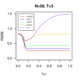
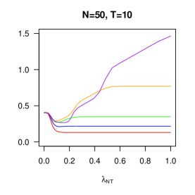
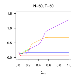
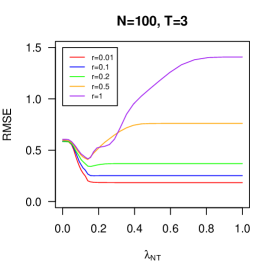
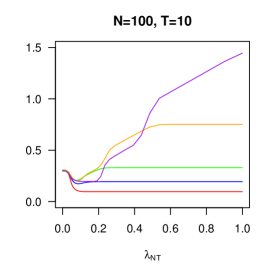
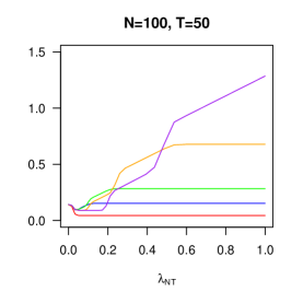
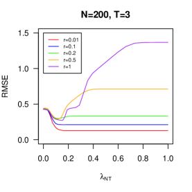
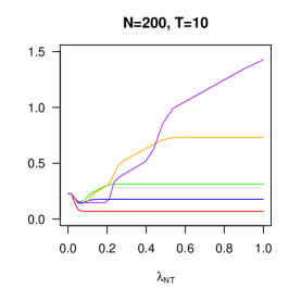
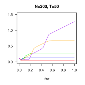
Figure 1: RMSE of penalized estimator with different sample sizes, degrees of nonlinearity and tuning parameter $\lambda_{NT}$.

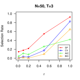
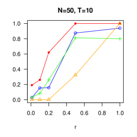
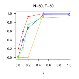
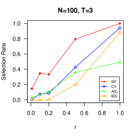
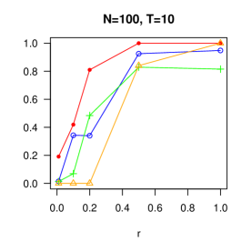
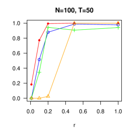
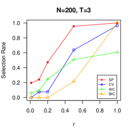
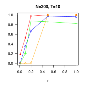
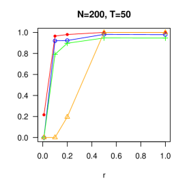
Figure 2: Proportion of correct linearity identification with different sample sizes and degrees of nonlinearity. SP stands for the proportion of solution path containing the correct model. CV, AIC and BIC are the proportions of correct model selection from solution path based on 5-fold cross-validation, AIC and BIC, respectively.

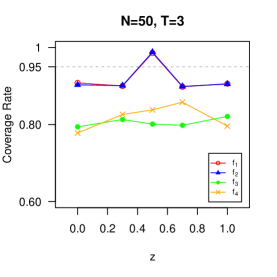
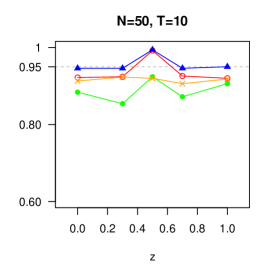
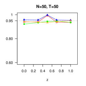
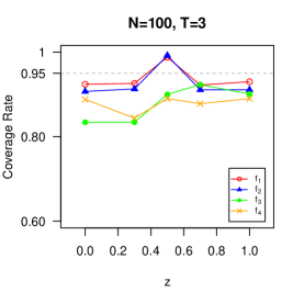
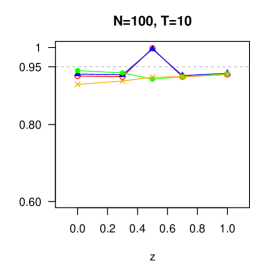
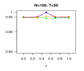
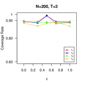
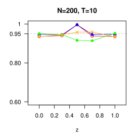
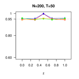
Figure 3: Coverage rates of the $95\%$ confidence intervals for $f_{j,0}(z_{0})$’s with different sample sizes and $r=1$.

7 Empirical Application

7.1 Aggregate Production

In this section, we apply our linearity detection procedure to Aggregate Production data, which is extracted from version 9.0 of the Penn World Table. We keep a balanced panel dataset for $48$ countries across the world for the period 1950-2014. Following Glass et al., (2016), we consider following regression model,

$$y_{it}=f_{1}(k_{it})+f_{2}(l_{it})+f_{3}(\textrm{pub}_{it})+f_{4}(\textrm{xm}_{it})+\alpha_{i}+error,$$

where $y_{it},k_{it},l_{it}$ are the real log GDP, capital stock, and number of people engaged of the $i$-th country at time $t$, respectively. Besides, $\textrm{pub}_{it}$ is government/public expenditure, defined as the government spending, and $\textrm{xm}_{it}$ is net trade openness, which equals exports minus imports of merchandise. Using the same criteria as in the simulation study, we choose $h_{1}=h_{2}=h_{3}=h_{4}=0.2$ by cross-validation. The tuning parameter $\lambda_{NT}$ is selected such that $\log(\lambda_{NT})$ increases from $-4$ to $-3$ with an increment $0.05$. Firstly, the solution path in Figure 4 indicates five candidate models can be obtained when $\lambda_{NT}$ increasing with models being summarized in Table 1. Moreover, according to Table 1, among these five candidates, the model with all linear $f_{j}$’s is the preferable based on CV. The estimated coefficients of explanatory variables are provided in Table 2, from which we can see the model is highly significant. Non-penalized estimators of $f_{j}$’s are constructed and corresponding fitted curves are provided in Figure 5. The fitted curves of the non-penalized estimators preserve linear patterns if one only looks at the interval between two dashed vertical lines, which is the $2.5\%$ to $97.5\%$ percentile range of the corresponding regressor. This information contained in Figure 5 coincides with the findings based on our proposed linearity detection procedure.

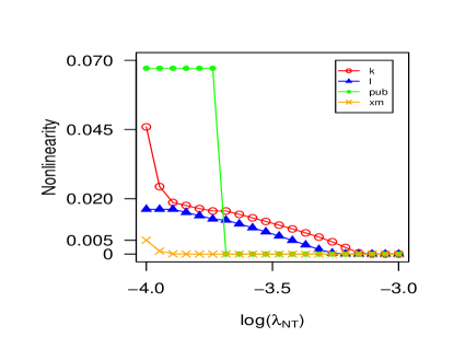
Figure 4: Solution Path of nonlinearity.

	Model 1	Model 2	Model 3	Model 4	Model 5
Linearity	$\emptyset$	xm	pub,xm	l,pub,xm	k,l,pub,xm
CV	2.616	1.453	0.054	0.042	0.040*

Table 1: Models selected by solution path.

	k	l	pub	xm
Coef	7.627∗∗∗	2.187∗∗∗	0.668∗∗∗	0.586∗∗∗
SE	0.178	0.426	0.230	0.122

Table 2: Linear Coefficients Estimators for Aggregate Production

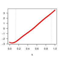
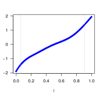
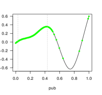
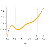
Figure 5: Estimated curves of $f_{j}$’s. Non-penalized estimator for top 4 panels; Penalized estimator for bottom 4 panels. Two vertical dashed lines indicates the $2.5\%$ to $97.5\%$ pencentile range of each regressor.

7.2 Environmental Kuznets Curve

In the second application, we estimate the environmental Kuznets curve (EKC), which is also studied in Ang, (2007), Apergis and Payne, (2009) and Li et al., (2016). Following Li et al., (2016), we consider the following nonparametric model:

$$y_{it}=f_{1}(\textrm{e}_{it})+f_{2}(\textrm{gdp}_{it})+f_{3}(\textrm{trade}_{it})+\alpha_{i}+\epsilon_{it},$$ (7.1)

where $y_{it}$ represents the per capita $\textrm{CO}_{2}$ emission of country $i$ in year $t$, $\textrm{e}_{it}$ is per capita energy consumption, $\textrm{gdp}_{it}$ stands for the per capita GDP, and $\textrm{trade}_{it}$ is the per capta trade. All the variables are taken logarithm and all the explanatory variables are scaled to $[0,1]$. The data is obtained from World Bank Development Indicators and we keep a balanced panel for $N=89$ and $T=40$ after eliminating missing values.

From the solution path in Figure 6, we extract 4 submodels and calculate their CV scores, which are summarized in Table 3. Based on the CV score, the selected linear explanatory variables are trade and e, while the variable gpd will be treated as nonlinear. Based on selected, model, we further estimate the linear and nonlinear components, and the results are reported in Table 4 and Figure 8. Table 4 shows the coefficients of e and trade are both highly significant. Meanwhile, Figure 8 indicates that as gdp increasing, its effect on $\textrm{CO}_{2}$ emission will increases first and then begin to fall, which coincides with common hypothesis that the relationship between income and the emission of chemicals like sulfur dioxide ($\textrm{SO}_{2}$) and carbon dioxide ($\textrm{CO}_{2}$) or the natural resource usage has an inverted U-shape, see Li et al., (2016). Finally, we present the nonpenalized estimation curves of the explanatory variables in Figure 7. If only screening the fitted curves in $2.5\%$ to $97.5\%$ pencentile range of the regressors in Figure 7, we can draw the same conclusion that e and trade are linear, while gdp is nonlinearly correlated with CO₂ emission.

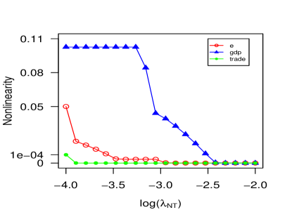
Figure 6: Solution Path of nonlinearity.

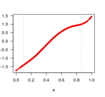
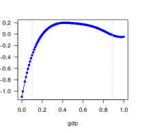
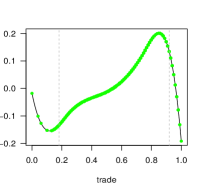
Figure 7: Estimated curves of $f_{j}$’s. Non-penalized estimator for top 4 panels; Penalized estimator for bottom 4 panels. Two vertical dashed lines indicates the $5\%$ to $95\%$ pencentile range of each regressor.

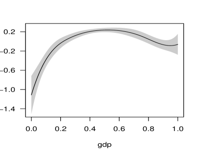
Figure 8: Confidence interval of $f_{2}$

	Model 1	Model 2	Model 3	Model 4
Linearity	$\emptyset$	trade	trade,e	trade,e,gdp
CV	0.0541	0.0523	0.0489∗	0.0563

Table 3: CV Scores of Models in Solution Path for EKC

	e	trade
Coef	3.452∗∗∗	0.491∗∗∗
SE	0.303	0.123

Table 4: Linear Coefficients Estimators for EKC

Appendix

This appendix contains proofs and simulation results which are not included in the main text. For simplicity, we define following notation. For function $g\mathrel{\mathop{\mathchar 58\relax}}\mathcal{Z}\to\mathbb{R}$, define $\mathbb{E}_{i}(g)=\mathbb{E}(g(\mathbf{Z}_{i1}))$ when ever the expected value exists. Define $\Theta_{NT,j}=\textrm{CSpl}(r_{j},\mathbf{t}_{j,M_{j}})$, the Centralized Spline Space to approximate $f_{j}$, for $j\in[p]$, and denote $\Theta_{NT,j,-},\Theta_{NT,j,\sim}$ as the subspaces of $\Theta_{NT,j}$ for linear and nonlinear component respectively. By this notation and for any $g\in\Theta_{NT,j}$, we define $g_{-}\in\Theta_{NT,j,-}$ and $g_{\sim}\in\Theta_{NT,j,\sim}$ such that $g=g_{-}+g_{\sim}$, which is the unique decomposition due to (3.1). Recall that the function space of correct specified model is defined as

$$\Theta_{NT}^{0}=\bigg{\{}f(\mathbf{z})=\sum_{j=1}^{p}f_{j}(z_{j})\in\Theta_{NT}\;\bigg{|}\;f_{j}(z)=\beta_{j}(z-1/2)\textrm{ for }\beta_{j}\in\mathbb{R}\textrm{ and }j=1,\ldots,d\bigg{\}},$$

and we define its complement by the following:

$$\Theta_{NT}^{1}=\bigg{\{}f(\mathbf{z})=\sum_{j=1}^{d}f_{j}(z_{j})\;\bigg{|}\>f_{j}\in\Theta_{NT,j,\sim}\bigg{\}}.$$

We also define the non-penalized projection estimators as follows:

$$\widehat{f}_{*}=\operatorname*{argmin}_{f\in\Theta_{NT}}\|Y-f\|_{NT}^{2}\textrm{,\;\; }\widehat{f}_{*,0}=\operatorname*{argmin}_{f\in\Theta_{NT}^{0}}\|Y-f\|_{NT}^{2},$$

here $Y$ is treated as a function such that $Y(\mathbf{Z}_{it})=Y_{it}$. Let $\|\cdot\|_{\infty}$ be the sup-norm of a function, and $\lambda_{\min}(A),\;\lambda_{\max}(A)$ be the smallest, and largest eigenvalues of squared matrix $A$.

In the following, we need introduce notation for vectors for convenience. We define $\bm{\epsilon}=(\epsilon_{11},\epsilon_{12},\ldots,\epsilon_{it},\ldots,\epsilon_{NT})^{\top}\in\mathbb{R}^{NT}$, and for any $f\mathrel{\mathop{\mathchar 58\relax}}\mathcal{Z}\to\mathbb{R}$, we denote the bold-faced $\mathbf{f}$ as the vector $\mathbf{f}=(f(\mathbf{Z}_{11}),f(\mathbf{Z}_{12}),\ldots,f(\mathbf{Z}_{it}),\ldots,f(\mathbf{Z}_{NT}))^{\top}\in\mathbb{R}^{NT}$. By this definition, we have $\bm{\epsilon}=\mathbf{Y}-\mathbf{f}_{0}$.

We also define following sequences which will be frequently used in the proof:

• $d_{NT}$: the dimension of $\Theta_{NT}$ and $d_{NT}\asymp\sum_{j=1}^{p}h_{j}^{-1}$;

• $d_{NT,0}$: the dimension of $\Theta_{NT}^{0}$ and $d_{NT}\asymp\sum_{j=d+1}^{p}h_{j}^{-1}$;

• $A_{NT}$: a constant such that $\|f\|_{\infty}\leq A_{NT}\|f\|_{2}$ for all $f\in\Theta_{NT}$ and $A_{NT}^{2}\asymp\sum_{j=1}^{p}h_{j}^{-1}$, see Lemma A.2;

• $A_{NT,0}$: a constant such that $\|f\|_{\infty}\leq A_{NT}\|f\|_{2}$ for all $f\in\Theta_{NT}^{0}$ and $A_{NT,0}^{2}\asymp\sum_{j=d+1}^{p}h_{j}^{-1}$, see Lemma A.2;

• $\rho_{NT}$: approximation error bound and $\rho_{NT}\asymp\sum_{j=d+1}^{p}h_{j}^{m_{j}}$, see Lemma A.4;

• $\gamma_{NT}$: $\gamma_{NT}^{2}=\sum_{j=1}^{p}(NTh_{j})^{-1}+\sum_{j=d+1}^{p}h_{j}^{2m_{j}}$.

A.1 Proof of Theorems 1 and 2 – Fixed $T$ Case

Lemma A.1.

Under Assumption A1, the following holds for all $g\in\mathcal{H}$:

$$\frac{1}{2a_{1}}\|g\|_{2}^{2}\leq\mathbb{E}\bigg{(}\zeta_{i}(g,g)\bigg{)}\leq a_{1}\|g\|_{2}^{2},\textrm{ and }\;\;\frac{1}{2a_{1}}\|g\|_{2}^{2}\leq\|g\|^{2}\leq a_{1}\|g\|_{2}^{2}.$$

Moreover, if $g\in\mathcal{H}^{0}$, we have

$$\frac{1}{a_{1}}\|g\|_{2}^{2}\leq\mathbb{E}\bigg{(}g^{2}(\mathbf{Z}_{it})\bigg{)}\leq a_{1}\|g\|_{2}^{2}.$$

Proof of Lemma A.1.

We only derive the upper bound, since the lower bounded can be obtained analogically. By Assumption A1 and direct examination, we have

$$\mathbb{E}\bigg{(}\zeta_{i}(g,g)\bigg{)} = \mathbb{E}\bigg{\{}\frac{1}{T}\sum_{t=1}^{T}\bigg{(}g(\mathbf{Z}_{it})-\frac{1}{T}\sum_{s=1}^{T}g(\mathbf{Z}_{is})\bigg{)}^{2}\bigg{\}}$$

$$= \int\frac{1}{T}\sum_{t=1}^{T}\bigg{(}g(\mathbf{z}_{it})-\frac{1}{T}\sum_{s=1}^{T}g(\mathbf{z}_{is})\bigg{)}^{2}q_{i}(\mathbf{w}_{i})d\mathbf{w}_{i}$$

$$\leq a_{1}\int\frac{1}{T}\sum_{t=1}^{T}\bigg{(}g(\mathbf{z}_{it})-\frac{1}{T}\sum_{s=1}^{T}g(\mathbf{z}_{is})\bigg{)}^{2}d\mathbf{w}_{i}$$

$$= \frac{a_{1}(T-1)}{T}\bigg{\{}\int g^{2}(\mathbf{z})d\mathbf{z}-\bigg{(}\int g(\mathbf{z})d\mathbf{z}\bigg{)}\bigg{\}}$$

$$\leq a_{1}\|g\|_{2}^{2}$$

which is the upper bound. By similar argument, we can show that

$$\mathbb{E}\bigg{(}\zeta_{i}(g,g)\bigg{)} = \mathbb{E}\bigg{\{}\frac{1}{T}\sum_{t=1}^{T}\bigg{(}g(\mathbf{Z}_{it})-\frac{1}{T}\sum_{s=1}^{T}g(\mathbf{Z}_{is})\bigg{)}^{2}\bigg{\}}$$

$$= \int\frac{1}{T}\sum_{t=1}^{T}\bigg{(}g(\mathbf{z}_{it})-\frac{1}{T}\sum_{s=1}^{T}g(\mathbf{z}_{is})\bigg{)}^{2}q_{i}(\mathbf{w}_{i})d\mathbf{w}_{i}$$

$$\geq a_{1}^{-1}\int\frac{1}{T}\sum_{t=1}^{T}\bigg{(}g(\mathbf{z}_{it})-\frac{1}{T}\sum_{s=1}^{T}g(\mathbf{z}_{is})\bigg{)}^{2}d\mathbf{w}_{i}$$

$$= \frac{a_{1}^{-1}(T-1)}{T}\bigg{\{}\int g^{2}(\mathbf{z})d\mathbf{z}-\bigg{(}\int g(\mathbf{z})d\mathbf{z}\bigg{)}\bigg{\}}$$

$$\leq \frac{1}{2a_{1}}\|g\|_{2}^{2}$$

where we used the fact that $2(T-1)\geq T$. Notice $\|g\|^{2}=\frac{1}{N}\sum_{i=1}^{N}\mathbb{E}(\zeta_{i}(g,g))$, we prove the second inequality. For the last in equality, the proof is similar and we omit it. ∎

Lemma A.2.

Under Assumption A1 and A3, $\|g\|_{\infty}\leq A_{NT}\|g\|_{2}$, for all $g\in\Theta_{NT}$, and $\|g\|_{\infty}\leq A_{NT,0}\|g\|_{2}$ for all $g\in\Theta_{NT}^{0}$, where $A_{NT}\asymp\sum_{j=1}^{p}h_{j}^{-1/2}$, and $A_{NT,0}\asymp\sum_{j=d+1}^{p}h_{j}^{-1/2}$.

Proof of Lemma A.2.

We only prove the first inequality, as the second one can be proved similarly. Suppose $g=\sum_{j=1}^{p}g_{j}$ with $g_{j}\in\Theta_{{NT},j}$, by DeVore and Lorentz, (1993)[Theorem 5.1.2], it follows that

$$\|g_{j}\|_{\infty}\leq r_{j}\|g\|_{2},\textrm{ with }r_{j}\asymp h_{j}^{-1/2},\textrm{ for }j=1,2,\ldots p.$$

By Lemma A.3 and above inequality, we have

$$\|g\|_{\infty}\leq\sum_{j=1}^{p}\|g_{j}\|_{\infty}\leq\sum_{j=1}^{p}r_{j}\|g_{j}\|_{2}\leq c^{-1}\sum_{j=1}^{p}r_{j}\|g\|_{2}.$$

∎

Lemma A.3.

Suppose one of the following conditions is satisfied:

1. Assumptions A1 and A3 are valid;

2. Assumptions A3 and A2 hold and $A_{NT}^{2}=o(T)$.

Then there exists $c_{1}>0$ depending on $a_{1},a_{3},p$ such that

$$\|g\|_{2}^{2}\geq c_{1}\sum_{j=1}^{p}\|g_{j}\|_{2}^{2}\textrm{ and }\;\|g\|^{2}\geq c_{1}\sum_{j=1}^{p}\|g_{j}\|^{2},$$

for all $g=\sum_{j=1}^{p}g_{j}\in\Theta_{NT}$ with $g_{j}\in\Theta_{{NT},j},j=1,2,\ldots,p$.

Proof of Lemma A.3.

First inequality is essentially Stone, (1994)[Lemma 3.1] and the second one follows from Lemma A.1 for fixed $T$ and Lemma A.12 for diverging $T$. ∎

Lemma A.4.

Under Assumption A3, there exist $g_{*}=\sum_{j=1}^{p}g_{j,*}\in\Theta_{NT}^{0}$ with $g_{j,*}\in\Theta_{{NT},j}$ such that $g_{j,*}=f_{j,0}$ for $j=1,\ldots,d$, and $\|g_{j,*}-f_{j,0}\|_{\infty}\leq\rho_{NT,j}$ with $\rho_{NT,j}\asymp h_{j}^{m_{j}}$ for $j=d+1,\ldots,p$. As a consequence, it holds that $\|g_{*}-f_{0}\|_{\infty}\leq\rho_{NT}$ with $\rho_{NT}\asymp\sum_{j=d+1}^{p}h_{j}^{m_{j}}$.

Proof.

This a well known result, i.e., see Chen, (2007). ∎

Lemma A.5.

Under Assumption A1 and A3, if $d_{NT}A_{NT}^{2}=o(N)$, then

$$\mathbb{P}\bigg{(}\sup_{g,f\in\Theta_{NT}}\bigg{|}\frac{\langle f,g\rangle_{NT}-\langle f,g\rangle}{\|f\|_{2}\|g\|_{2}}\bigg{|}>x\bigg{)} \leq \frac{2}{e}\bigg{\{}\frac{128a_{1}A_{NT}^{2}}{Nx^{2}}\sum_{k=1}^{\infty}\bigg{(}\frac{9}{4}\bigg{)}^{k-1}+\frac{128a_{1}A_{NT}^{2}}{Nx}\sum_{k=1}^{\infty}\bigg{(}\frac{3}{2}\bigg{)}^{k-1}\bigg{\}}.$$

As a consequence, it follows that

$$\sup_{g,f\in\Theta_{NT}}\bigg{|}\frac{\langle f,g\rangle_{NT}-\langle f,g\rangle}{\|f\|_{2}\|g\|_{2}}\bigg{|}=o_{P}(1)\;\textrm{ and }\;\sup_{g,f\in\Theta_{NT}}\bigg{|}\frac{\langle f,g\rangle_{NT}-\langle f,g\rangle}{\|f\|\|g\|}\bigg{|}=o_{P}(1).$$

Moreover, we also have

$$\sup_{g,f\in\Theta_{NT}}\bigg{|}\frac{\frac{1}{NT}\sum_{i=1}^{N}\sum_{t=1}^{T}g(\mathbf{Z}_{it})f(\mathbf{Z}_{it})-\frac{1}{N}\sum_{i=1}^{N}\mathbb{E}_{i}(gf)}{\|g\|_{2}\|f\|_{2}}\bigg{|}=o_{P}(1).$$

Proof of Lemma A.5.

Let $\mathcal{F}_{\textrm{UB}}^{0}=\{f\in\Theta_{NT}\mathrel{\mathop{\mathchar 58\relax}}\|f\|_{2}\leq 1\}$, $\Theta=\mathcal{F}_{\textrm{UB}}^{0}\times\mathcal{F}_{\textrm{UB}}^{0}$ and

$$\xi_{i}(\theta) = \frac{1}{T}\sum_{t=1}^{T}\bigg{(}g(\mathbf{Z}_{it})-\frac{1}{T}\sum_{s=1}^{T}g(\mathbf{Z}_{is})\bigg{)}\bigg{(}f(\mathbf{Z}_{it})-\frac{1}{T}\sum_{s=1}^{T}f(\mathbf{Z}_{is})\bigg{)},\textrm{ with }\theta=(g,f),$$

$$X_{i}(\theta) = {\xi_{i}(\theta)-\mathbb{E}(\xi_{i}(\theta))},\;\;\;\;S_{N}(\theta)=\frac{1}{N}\sum_{i=1}^{N}X_{i}(\theta)$$

Define metric on $\Theta$ by $d(\theta_{1},\theta_{2})=\sqrt{\|g_{1}-g_{2}\|_{2}^{2}/2+\|f_{1}-f_{2}\|_{2}^{2}/2}$ for $\theta_{1}=(g_{1},f_{1}),\theta_{2}=(g_{2},f_{2})\in\mathcal{F}_{\textrm{UB}}^{0}\times\mathcal{F}_{\textrm{UB}}^{0}$. Moreover, by Lemma A.2, we have

$$|\xi_{i}(\theta_{1})-\xi_{i}(\theta_{2})|$$

$$\leq \bigg{|}\frac{1}{T}\sum_{t=1}^{T}\bigg{(}g_{1}(\mathbf{Z}_{it})-g_{2}(\mathbf{Z}_{it})-\frac{1}{T}\sum_{s=1}^{T}g_{1}(\mathbf{Z}_{is})+\frac{1}{T}\sum_{s=1}^{T}g_{2}(\mathbf{Z}_{is})\bigg{)}\bigg{(}f_{1}(\mathbf{Z}_{it})-\frac{1}{T}\sum_{s=1}^{T}f_{1}(\mathbf{Z}_{is})\bigg{)}\bigg{|}$$

$$+\bigg{|}\frac{1}{T}\sum_{t=1}^{T}\bigg{(}f_{1}(\mathbf{Z}_{it})-f_{2}(\mathbf{Z}_{it})-\frac{1}{T}\sum_{s=1}^{T}f_{1}(\mathbf{Z}_{is})+\frac{1}{T}\sum_{s=1}^{T}f_{2}(\mathbf{Z}_{is})\bigg{)}\bigg{(}g_{2}(\mathbf{Z}_{it})-\frac{1}{T}\sum_{s=1}^{T}g_{2}(\mathbf{Z}_{is})\bigg{)}\bigg{|}$$

$$\leq 4\|g_{1}-g_{2}\|_{\infty}\|f_{1}\|_{\infty}+4\|f_{1}-f_{2}\|_{\infty}\|g_{2}\|_{\infty}$$

$$\leq 4A_{NT}^{2}\|g_{1}-g_{2}\|_{2}\|f_{1}\|_{2}+4A_{NT}^{2}\|f_{1}-f_{2}\|_{2}\|g_{2}\|_{2}$$

$$\leq 8A_{NT}^{2}d(\theta_{1},\theta_{2}),$$

which further leads to

$$|X_{i}(\theta_{1})-X_{i}(\theta_{2})|\leq 16A_{{NT}}^{2}d(\theta_{1},\theta_{2}).$$

Similarly, by Lemma A.1 and Lemma A.2, we have

$$\textrm{Var}\bigg{(}X_{i}(\theta_{1})-X_{i}(\theta_{2})\bigg{)}$$

$$\leq \mathbb{E}\bigg{(}|\xi_{i}(\theta_{1})-\xi_{i}(\theta_{2})|^{2}\bigg{)}$$

$$\leq 8\|f_{1}\|_{\infty}^{2}\mathbb{E}\bigg{\{}\frac{1}{T}\sum_{t=1}^{T}\bigg{(}g_{1}(\mathbf{Z}_{it})-g_{2}(\mathbf{Z}_{it})-\frac{1}{T}\sum_{s=1}^{T}g_{1}(\mathbf{Z}_{is})+\frac{1}{T}\sum_{s=1}^{T}g_{2}(\mathbf{Z}_{is})\bigg{)}^{2}\bigg{\}}$$

$$+8\|g_{2}\|_{\infty}^{2}\mathbb{E}\bigg{\{}\frac{1}{T}\sum_{t=1}^{T}\bigg{(}f_{1}(\mathbf{Z}_{it})-f_{2}(\mathbf{Z}_{it})-\frac{1}{T}\sum_{s=1}^{T}f_{1}(\mathbf{Z}_{is})+\frac{1}{T}\sum_{s=1}^{T}f_{2}(\mathbf{Z}_{is})\bigg{)}^{2}\bigg{\}}$$

$$= 8\|f_{1}\|_{\infty}^{2}\mathbb{E}\bigg{(}\zeta_{i}(g_{1}-g_{2},g_{1}-g_{2})\bigg{)}+8\|g_{2}\|_{\infty}^{2}\mathbb{E}\bigg{(}\zeta_{i}(f_{1}-f_{2},f_{1}-f_{2})\bigg{)}$$

$$\leq 8A_{NT}^{2}\bigg{(}\|f_{1}\|_{2}^{2}\|g_{1}-g_{2}\|^{2}+\|g_{2}\|_{2}^{2}\|f_{1}-f_{2}\|^{2}\bigg{)}$$

$$\leq 8a_{1}A_{NT}^{2}\bigg{(}\|f_{1}\|_{2}^{2}\|g_{1}-g_{2}\|_{2}^{2}+\|g_{2}\|_{2}^{2}\|f_{1}-f_{2}\|_{2}^{2}\bigg{)}$$

$$\leq 16a_{1}A_{NT}^{2}d^{2}(\theta_{1},\theta_{2}).$$

By Bernstein inequality, it follows that

$$\mathbb{P}\bigg{(}\bigg{|}S_{N}(\theta_{1})-S_{N}(\theta_{2})\bigg{)}\bigg{|}>xs\bigg{)} \leq 2\exp\bigg{(}-\frac{Nx^{2}s^{2}}{32a_{1}A_{NT}^{2}\{d^{2}(\theta_{1},\theta_{2})+d(\theta_{1},\theta_{2})xs\}}\bigg{)}$$

$$\leq 2\exp\bigg{(}-\frac{Nx^{2}s^{2}}{64a_{1}A_{NT}^{2}d^{2}(\theta_{1},\theta_{2})}\bigg{)}+2\exp\bigg{(}-\frac{Nxs}{64a_{1}A_{NT}^{2}d(\theta_{1},\theta_{2})}\bigg{)}.$$

Let $\delta_{k}=3^{-k}$ for $k\geq 0$. For sufficient large integer $K$, which will be specified later, let $\{0\}=\mathcal{H}_{0}\subset\mathcal{H}_{1}\ldots\mathcal{H}_{K}$ be a sequence of subsets of $\Theta$ such that $\min_{\theta^{*}\in\mathcal{H}_{k}}d(\theta^{*},\theta)\leq\delta_{k}$ for all $\theta\in\Theta$. Moreover the subsets $\mathcal{H}_{K}$ is chosen inductively such that two different elements in $\mathcal{H}_{k}$ is at least $\delta_{k}$ apart.

By definition, the cardinality $\#(\mathcal{H}_{k})$ of $\mathcal{H}_{k}$ is bounded by the $\delta_{k}/2$-covering number $D(\delta_{k}/2,\Theta,d)$. Moreover, since $d(\theta_{1},\theta_{2})\leq\|g_{1}-g_{2}\|_{2}+\|f_{1}-f_{2}\|_{2}$ for $\theta_{1}=(g_{1},f_{1}),\theta_{2}=(g_{2},f_{2})\in\Theta$, we have

$$D(\delta_{k}/2,\Theta,d)\leq D^{2}(\delta_{k}/4,\mathcal{F}_{\textrm{UB}}^{0},\|\cdot\|_{2})\leq\bigg{(}\frac{16+\delta_{k}}{\delta_{k}}\bigg{)}^{2d_{NT}},$$

where the last inequality is due to Van de Geer, (2000)[Corollary 2.6] and the fact that $\mathcal{F}_{\textrm{UB}}^{0}$ is a linear space with dimension $d_{NT}$. For any $\theta\in\Theta$, let $\tau_{k}(\theta)\in\mathcal{H}_{k}$ be a element such that $d(\tau_{k}(\theta),\theta)\leq\delta_{k}$, for $k=1,2,\ldots,K$. Now for fixed $x>0$, choose $K=K(N)>0$, which depends on $N$ and is increasing fast enough such that $x>16A_{NT}^{2}(2/3)^{K}$, we see from (LABEL:eq:lemma:uniform:equivalence:empirical:population:norm:eq1) that

$$\mathbb{P}\bigg{(}\sup_{\theta\in\Theta}\bigg{|}S_{N}(\theta)\bigg{|}>x\bigg{)}$$ (A.2)

$$\leq \mathbb{P}\bigg{(}\sup_{\theta\in\Theta}\bigg{|}S_{N}(\theta)-S_{N}\bigg{(}\tau_{K}(\theta)\bigg{)}\bigg{|}>\frac{x}{2^{K}}\bigg{)}$$

$$+\sum_{k=1}^{K}\mathbb{P}\bigg{(}\sup_{\theta\in\Theta}\bigg{|}S_{N}\bigg{(}\tau_{k}\circ\ldots\circ\tau_{K}(\theta)\bigg{)}-S_{N}\bigg{(}\tau_{k-1}\circ\tau_{k}\circ\ldots\circ\tau_{K}(\theta)\bigg{)}\bigg{|}>\frac{x}{2^{k-1}}\bigg{)}$$

$$\leq \mathbb{P}\bigg{(}16A_{NT}^{2}d(\theta,\tau_{K}(\theta))>\frac{x}{2^{K}}\bigg{)}$$

$$+\sum_{k=1}^{K}\#(\mathcal{H}_{k})\sup_{\theta_{k}\in\mathcal{H}_{k}}\mathbb{P}\bigg{(}\sup_{\theta\in\Theta}\bigg{|}S_{N}\bigg{(}\theta_{k}\bigg{)}-S_{N}\bigg{(}\tau_{k-1}(\theta_{k})\bigg{)}\bigg{|}>\frac{x}{2^{k-1}}\bigg{)}$$

$$\leq 0+\sum_{k=1}^{K}\bigg{(}\frac{16+3^{-k}}{3^{-k}}\bigg{)}^{2d_{NT}}\sup_{\theta_{k}\in\mathcal{H}_{k}}\mathbb{P}\bigg{(}\sup_{\theta\in\Theta}\bigg{|}S_{N}\bigg{(}\theta_{k}\bigg{)}-S_{N}\bigg{(}\tau_{k-1}(\theta_{k})\bigg{)}\bigg{|}>\frac{x}{2^{k-1}}\bigg{)}$$

$$\leq \sum_{k=1}^{K}2\bigg{(}\frac{16+3^{-k}}{3^{-k}}\bigg{)}^{2d_{NT}}\exp\bigg{(}-\frac{Nx^{2}}{64a_{1}A_{NT}^{2}2^{2(k-1)}d^{2}(\theta_{k},\tau_{k-1}(\theta_{k}))}\bigg{)}$$

$$+\sum_{k=1}^{K}2\bigg{(}\frac{16+3^{-k}}{3^{-k}}\bigg{)}^{2d_{NT}}\exp\bigg{(}-\frac{Nx}{64a_{1}A_{NT}^{2}2^{k-1}d(\theta_{k},\tau_{k-1}(\theta_{k}))}\bigg{)}$$

$$\leq \sum_{k=1}^{K}2\bigg{(}\frac{16+3^{-k}}{3^{-k}}\bigg{)}^{2d_{NT}}\exp\bigg{(}-\frac{Nx^{2}}{64a_{1}A_{NT}^{2}}\bigg{(}\frac{3}{2}\bigg{)}^{2(k-1)}\bigg{)}$$

$$+\sum_{k=1}^{\infty}2\bigg{(}\frac{16+3^{-k}}{3^{-k}}\bigg{)}^{2d_{NT}}\exp\bigg{(}-\frac{Nx}{64a_{1}A_{NT}^{2}}\bigg{(}\frac{3}{2}\bigg{)}^{k-1}\bigg{)}$$

$$\leq 2\sum_{k=1}^{\infty}\exp\bigg{(}4(3+k)d_{NT}-\frac{Nx^{2}}{64a_{1}A_{NT}^{2}}\bigg{(}\frac{9}{4}\bigg{)}^{k-1}\bigg{)}$$

$$+2\sum_{k=1}^{\infty}\exp\bigg{(}4(3+k)d_{NT}-\frac{Nx}{64a_{1}A_{NT}^{2}}\bigg{(}\frac{3}{2}\bigg{)}^{k-1}\bigg{)},$$

where we used the fact that $16\times 3^{k}+1\leq 3^{k+3}$ and $\log 3\leq 2$. Now choose $N$ large enough such that

$$512(3+k)a_{1}A_{NT}^{2}d_{NT}<Nx^{2}(9/4)^{k-1}\;\textrm{ and }\;\;512(3+k)a_{1}A_{NT}^{2}d_{NT}<N(3/2)^{k-1}x,$$ (A.3)

for all $k\geq 0$, which is possible, since $d_{NT}A_{NT}^{2}=o(N)$. For all $N$ large enough satisfying (A.2), (A.3) further leads to

$$\mathbb{P}\bigg{(}\sup_{\theta\in\Theta}\bigg{|}S_{N}(\theta)\bigg{|}>x\bigg{)} \leq 2\sum_{k=1}^{\infty}\exp\bigg{(}-\frac{Nx^{2}}{128a_{1}A_{NT}^{2}}\bigg{(}\frac{9}{4}\bigg{)}^{k-1}\bigg{)}+2\sum_{k=1}^{\infty}\exp\bigg{(}-\frac{Nx}{128a_{1}A_{NT}^{2}}\bigg{(}\frac{3}{2}\bigg{)}^{k-1}\bigg{)}$$

$$\leq \frac{2}{e}\bigg{\{}\frac{128a_{1}A_{NT}^{2}}{Nx^{2}}\sum_{k=1}^{\infty}\bigg{(}\frac{9}{4}\bigg{)}^{k-1}+\frac{128a_{1}A_{NT}^{2}}{Nx}\sum_{k=1}^{\infty}\bigg{(}\frac{3}{2}\bigg{)}^{k-1}\bigg{\}}\to 0,\textrm{ as }N\to\infty,$$

where the fact that $A_{NT}^{2}=o(N)$ and inequality $e^{-x}\leq e^{-1}/x$ are used. Notice that

$$\sup_{\theta\in\Theta}\bigg{|}S_{N}(\theta)\bigg{|}=\sup_{g,f\in\Theta_{NT}}\bigg{|}\frac{\langle f,g\rangle_{NT}-\langle f,g\rangle}{\|f\|_{2}\|g\|_{2}}\bigg{|},$$

we prove the first result. The second result is also valid according to Lemma A.1. Since the proof of third result is similar to previous two, we omit the proof. ∎

Lemma A.6.

Under Assumption A1 and A3, for element $v_{N}\in\mathcal{H}$, if $\|v_{N}\|_{\infty}<\infty$, then the following holds:

$$\mathbb{E}\bigg{(}\sup_{g\in\Theta_{NT}}\bigg{|}\frac{\langle v_{N},g\rangle_{NT}-\langle v_{N},g\rangle}{\|g\|}\bigg{|}^{2}\bigg{)}\leq 4\|v_{N}\|_{\infty}^{2}\frac{d_{NT}}{N},$$

and

$$\mathbb{E}\bigg{(}\sup_{g\in\Theta_{NT}}\bigg{|}\frac{\langle v_{N},g\rangle_{NT}-\langle v_{N},g\rangle}{\|g\|_{2}}\bigg{|}^{2}\bigg{)}\leq 4a_{1}^{2}\|v_{N}\|_{\infty}^{2}\frac{d_{NT}}{N}.$$

Proof of Lemma A.6.

Let $\{\chi_{j}\}_{j=1}^{d_{NT}}$ be the orthonormal basis of $\Theta_{NT}$ with respect to $\langle\cdot,\cdot\rangle$. For $g\in\Theta_{NT}$, we can rewrite $g=\sum_{j=1}^{d_{NT}}b_{j}\chi_{j}$ and $\|g\|^{2}=\sum_{j=1}^{d_{NT}}b_{j}^{2}$ with $b_{j}=\langle g,\chi_{j}\rangle\in\mathbb{R}$.

$$|\langle v_{N},g\rangle_{NT}-\langle v_{N},g\rangle| = \bigg{|}\sum_{j=1}^{d_{NT}}b_{j}\bigg{(}\langle v_{N},\chi_{j}\rangle_{NT}-\langle v_{N},\chi_{j}\rangle\bigg{)}\bigg{|}$$

$$\leq \bigg{(}\sum_{j=1}^{d_{NT}}b_{j}^{2}\bigg{)}^{1/2}\bigg{\{}\sum_{j=1}^{d_{NT}}\bigg{(}\langle v_{N},\chi_{j}\rangle_{NT}-\langle v_{N},\chi_{j}\rangle\bigg{)}^{2}\bigg{\}}^{1/2}$$

$$= \|g\|\bigg{\{}\sum_{j=1}^{d_{NT}}\bigg{(}\langle v_{N},\chi_{j}\rangle_{NT}-\langle v_{N},\chi_{j}\rangle\bigg{)}^{2}\bigg{\}}^{1/2},$$

which leads to

$$\sup_{g\in\Theta_{NT}}\bigg{|}\frac{\langle v_{N},g\rangle_{NT}-\langle v_{N},g\rangle}{\|g\|}\bigg{|}\leq\bigg{\{}\sum_{j=1}^{d_{NT}}\bigg{(}\langle v_{N},\chi_{j}\rangle_{NT}-\langle v_{N},\chi_{j}\rangle\bigg{)}^{2}\bigg{\}}^{1/2}.$$ (A.4)

Notice for each $j\in[d_{NT}]$, it follows that

$$\mathbb{E}\bigg{\{}\bigg{(}\langle v_{N},\chi_{j}\rangle_{NT}-\langle v_{N},\chi_{j}\rangle\bigg{)}^{2}\bigg{\}}=\textrm{Var}\bigg{(}\langle v_{N},\chi_{j}\rangle_{NT}\bigg{)} = \textrm{Var}\bigg{(}\frac{1}{N}\sum_{i=1}^{N}\zeta_{i}(v_{N},\chi_{j})\bigg{)}$$

$$= \frac{1}{N^{2}}\sum_{i=1}^{N}\textrm{Var}\bigg{(}\zeta_{i}(v_{N},\chi_{j})\bigg{)}$$

$$\leq \frac{1}{N^{2}}\sum_{i=1}^{N}\mathbb{E}\bigg{(}\zeta_{i}^{2}(v_{N},\chi_{j})\bigg{)}$$

$$\leq \frac{4\|v_{N}\|_{\infty}^{2}}{N^{2}}\sum_{i=1}^{N}\mathbb{E}\bigg{(}\zeta_{i}(\chi_{j},\chi_{j})\bigg{)}$$

$$= \frac{4\|v_{N}\|_{\infty}^{2}}{N}\|\chi_{j}\|^{2}=\frac{4\|v_{N}\|_{\infty}^{2}}{N}.$$

As a consequence, by taking expectation on both side of (A.4) and applying Cauchy–Schwarz inequality, we obtain the first result. The second result follows from the first one and Lemma A.1. ∎

Define event $\Omega_{N}=\{\mathbb{X}\mathrel{\mathop{\mathchar 58\relax}}1/2\|g\|\leq\|g\|_{NT}\leq 2\|g\|,\textrm{ for all }g\in\Theta_{NT}\}$ and $\mathbb{P}(\Omega_{N})\to 1$ as $N\to\infty$ by Lemma A.5. Then on event $\Omega_{N}$, $\langle\cdot,\cdot\rangle_{NT}$ is a valid inner product in $\Theta_{NT}$.

Lemma A.7.

Under Assumption A1 and A3, if $d_{NT}A_{NT}^{2}=o(N)$, then on event $\Omega_{N}$, the following holds,

$$\frac{a_{2}^{-1}d_{NT}}{NT}\leq\mathbb{E}\bigg{(}\|\widehat{f}_{*}-\widetilde{f}_{*}\|_{NT}^{2}\bigg{|}\mathbb{Z}\bigg{)}\leq\frac{a_{2}d_{NT}}{NT},$$

and

$$\mathbb{E}\bigg{(}\|\widehat{f}_{*}-f_{0}\|_{NT}^{2}\bigg{|}\mathbb{Z}\bigg{)}\geq\mathbb{E}\bigg{(}\|\widehat{f}_{*}-\widetilde{f}_{*}\|_{NT}^{2}\bigg{|}\mathbb{Z}\bigg{)}\geq\frac{a_{2}^{-1}d_{NT}}{NT}.$$

Proof of Lemma A.7.

On event $\Omega_{N}$, let $\{\phi_{j}\}_{j=1}^{d_{NT}}$ be the orthonormal basis of $\Theta_{NT}$ with respect to $\langle\cdot,\cdot\rangle_{NT}$. Recall $\widehat{f}_{*}=P_{NT}Y$, now we have

$$\widehat{f}_{*}-\widetilde{f}_{*} = \sum_{j=1}^{d_{NT}}\langle\widehat{f}_{*}-\widetilde{f}_{*},\phi_{j}\rangle_{NT}\phi_{j}$$

$$= \sum_{j=1}^{d_{NT}}\langle P_{NT}Y-P_{NT}f_{0},\phi_{j}\rangle_{NT}\phi_{j}$$

$$= \sum_{j=1}^{d_{NT}}\langle Y-f_{0},\phi_{j}\rangle_{NT}\phi_{j}.$$

By definition, it yields that

$$\langle Y-f_{0},\phi_{j}\rangle_{NT} = \frac{1}{NT}\sum_{i=1}^{N}\sum_{t=1}^{T}\bigg{\{}Y_{it}-f_{0}(\mathbf{Z}_{it})-\frac{1}{T}\sum_{s=1}^{T}\bigg{(}Y_{is}-f_{0}(\mathbf{Z}_{is})\bigg{)}\bigg{\}}\bigg{\{}\phi_{j}(\mathbf{Z}_{it})-\frac{1}{T}\sum_{s=1}^{T}\phi_{j}(\mathbf{Z}_{is})\bigg{\}}$$

$$= \frac{1}{N}\sum_{i=1}^{N}S_{ji},$$

where

$$S_{ji} = \frac{1}{T}\sum_{t=1}^{T}\bigg{(}\epsilon_{it}-\frac{1}{T}\sum_{s=1}^{T}\epsilon_{is}\bigg{)}\bigg{(}\phi_{j}(\mathbf{Z}_{it})-\frac{1}{T}\sum_{s=1}^{T}\phi_{j}(\mathbf{Z}_{is})\bigg{)}$$

$$= \frac{1}{T}\bm{\epsilon}_{i}^{\top}H{\Phi}_{ji},$$

where

$$\Phi_{ji} = \begin{pmatrix}\phi(\mathbf{Z}_{i1}),\phi(\mathbf{Z}_{i1}),\ldots,\phi(\mathbf{Z}_{iT})\end{pmatrix}^{\top}\in\mathbb{R}^{T},\;\;\bm{\epsilon}_{i}=(\epsilon_{i1},\epsilon_{i2},\ldots,\epsilon_{iT})^{\top}\in\mathbb{R}^{T},$$

$$H = I_{T}-\frac{1}{T}uu^{\top}\in\mathbb{R}^{T\times T},\textrm{ with }u=(1,1,\ldots,1)^{\top}\in\mathbb{R}^{T}.$$

Combining Assumption A3.(ii) and above equalities, we show that

$$\mathbb{E}(\widehat{f}_{*}|\mathbb{Z})=\widetilde{f}_{*}.$$

Moreover, Assumption A3.(ii) also implies $\mathbb{E}(S_{ji_{1}}S_{ji_{2}}|\mathbb{Z})=0$ when $i_{1}\neq i_{2}$ and

$$\mathbb{E}(S_{ji}^{2}|\mathbb{Z}) = \frac{1}{T^{2}}\mathbb{E}\bigg{(}\Phi_{ji}^{\top}H\bm{\epsilon}_{i}\bm{\epsilon}^{\top}H\Phi_{ji}\bigg{|}\mathbb{Z}\bigg{)}$$

$$= \frac{1}{T^{2}}\Phi_{ji}^{\top}H\mathbb{E}\bigg{(}\bm{\epsilon}_{i}\bm{\epsilon}^{\top}\bigg{|}\mathbb{Z}\bigg{)}H\Phi_{ji}$$

$$\leq \frac{a_{2}}{T^{2}}\Phi_{ji}^{\top}H\Phi_{ji}$$

$$= \frac{a_{2}}{T}\frac{1}{T}\sum_{t=1}^{T}\bigg{(}\phi_{j}(\mathbf{Z}_{it})-\frac{1}{T}\sum_{s=1}^{T}\phi_{j}(\mathbf{Z}_{is})\bigg{)}^{2}$$

Therefore, it follows that

$$\mathbb{E}(\|\widehat{f}_{*}-\widetilde{f}_{*}\|_{NT}^{2}|\mathbb{Z}) = \sum_{j=1}^{d_{NT}}\mathbb{E}(\langle Y-f_{0},\phi_{j}\rangle_{NT}^{2}|\mathbb{Z})$$

$$= \sum_{j=1}^{d_{NT}}\frac{1}{N^{2}}\sum_{i=1}^{N}\mathbb{E}(S_{ji}^{2}|\mathbb{Z})$$

$$\leq \frac{a_{2}}{N}\sum_{j=1}^{d_{NT}}\frac{1}{NT^{2}}\sum_{i=1}^{N}\sum_{t=1}^{T}\bigg{(}\phi_{j}(\mathbf{Z}_{it})-\frac{1}{T}\sum_{s=1}^{T}\phi_{j}(\mathbf{Z}_{is})\bigg{)}^{2}$$

$$= \frac{a_{2}}{NT}\sum_{j=1}^{d_{NT}}\|\phi_{j}\|_{NT}^{2}\leq\frac{a_{2}d_{NT}}{NT},\textrm{ for all }\mathbb{Z}\in\Omega_{N},$$

which is the upper bound. Similarly, utilizing Assumption A3.(ii) , we also can show that

$$\mathbb{E}(\|\widehat{f}_{*}-\widetilde{f}_{*}\|_{NT}^{2}|\mathbb{Z})\geq\frac{a_{2}^{-1}d_{NT}}{NT},\textrm{ for }\mathbb{Z}\in\Omega_{N}.$$

For second inequality, by definition of $\widetilde{f}_{*}$, on event $\Omega_{N}$, it follows that

$$\|\widehat{f}_{*}-f_{0}\|_{NT}^{2} = \|\widehat{f}_{*}-\widetilde{f}_{*}+\widetilde{f}_{*}-f_{0}\|_{NT}^{2}$$

$$= \|\widehat{f}_{*}-\widetilde{f}_{*}\|_{NT}^{2}+\|\widetilde{f}_{*}-f_{0}\|_{NT}^{2}+2\langle\widehat{f}_{*}-\widetilde{f}_{*},\widetilde{f}_{*}-f_{0}\rangle_{NT}$$

$$= \|\widehat{f}_{*}-\widetilde{f}_{*}\|_{NT}^{2}+\|\widetilde{f}_{*}-f_{0}\|_{NT}^{2}+2\langle P_{NT}Y-P_{NT}f_{0},P_{NT}f_{0}-f_{0}\rangle_{NT}$$

$$= \|\widehat{f}_{*}-\widetilde{f}_{*}\|_{NT}^{2}+\|\widetilde{f}_{*}-f_{0}\|_{NT}^{2}$$

$$\geq \|\widehat{f}_{*}-\widetilde{f}_{*}\|_{NT}^{2},$$

after taking conditional expectation, we finish the proof. ∎

Lemma A.8.

Suppose Assumption A1 and A3 hold and $d_{NT}A_{NT}^{2}=o(N)$, then on event $\Omega_{N}$, the following statements are true,

$$\mathbb{E}\bigg{(}\|\widehat{f}_{*}-f_{0}\|_{NT}^{2}\bigg{|}\mathbb{Z}\bigg{)}\leq 2500a_{2}^{2}\bigg{(}\frac{d_{NT}}{N}+\rho_{NT}^{2}\bigg{)},\;\;\mathbb{E}\bigg{(}\|\widehat{f}_{*}-f_{0}\|^{2}\bigg{|}\mathbb{Z}\bigg{)}\leq 2500a_{2}^{2}\bigg{(}\frac{d_{NT}}{N}+\rho_{NT}^{2}\bigg{)},$$

and

$$\mathbb{E}\bigg{(}\|\widehat{f}_{*,0}-f_{0}\|_{NT}^{2}\bigg{|}\mathbb{Z}\bigg{)}\leq 2500a_{2}^{2}\bigg{(}\frac{d_{NT,0}}{N}+\rho_{NT}^{2}\bigg{)},\;\mathbb{E}\bigg{(}\|\widehat{f}_{*,0}-f_{0}\|^{2}\bigg{|}\mathbb{Z}\bigg{)}\leq 2500a_{2}^{2}\bigg{(}\frac{d_{NT,0}}{N}+\rho_{NT}^{2}\bigg{)}.$$

Proof of Lemma A.8.

Let $\widetilde{f}_{*}=P_{NT}f_{0}$ and $\bar{f}_{*}=Pf_{0}$. Lemme A.7 implies that on event $\Omega_{N}$, it holds that

$$\frac{a_{2}^{-1}d_{NT}}{NT}\leq\|\widehat{f}_{*}-\widetilde{f}_{*}\|_{NT}^{2}\leq\frac{a_{2}d_{NT}}{NT},$$ (A.5)

Now by definition of $\Omega_{N}$, we have

$$\frac{a_{2}^{-1}d_{NT}}{4NT}\leq\|\widehat{f}_{*}-\widetilde{f}_{*}\|^{2}\leq\frac{4a_{2}d_{NT}}{NT}.$$ (A.6)

Next we will deal with $\widetilde{f}_{*}-\bar{f}_{*}$. By definition we have

$$\|\widetilde{f}_{*}-\bar{f}_{*}\|_{NT} = \sup_{g\in\Theta_{NT}}\bigg{|}\frac{\langle\widetilde{f}_{*}-\bar{f}_{*},g\rangle_{NT}}{\|g\|_{NT}}\bigg{|}$$

$$= \sup_{g\in\Theta_{NT}}\bigg{|}\frac{\langle P_{NT}f_{0}-Pf_{0},g\rangle_{NT}}{\|g\|_{NT}}\bigg{|}$$

$$= \sup_{g\in\Theta_{NT}}\bigg{|}\frac{\langle f_{0}-Pf_{0},g\rangle_{NT}-\langle f_{0}-Pf_{0},g\rangle}{\|g\|_{NT}}\bigg{|},$$

where the fact $\langle f_{0}-Pf_{0},g\rangle=0$ is used. Let $g_{*}\in\Theta_{NT}$ satisfy that $\|g_{*}-f_{0}\|_{\infty}\leq\rho_{NT}$, where the existence of such $g_{*}$ is guaranteed by Lemma A.4. Since

$$\langle f_{0}-Pf_{0},g\rangle_{NT}-\langle f_{0}-Pf_{0},g\rangle=\langle f_{0}-g_{*},g\rangle_{NT}-\langle f_{0}-g_{*},g\rangle+\langle g_{*}-Pf_{0},g\rangle_{NT}-\langle g_{*}-Pf_{0},g\rangle,$$

we have $\|\widetilde{f}_{*}-\bar{f}_{*}\|_{NT}\leq R_{1}+R_{2}+R_{3}$, where

$$R_{1} = \sup_{g\in\Theta_{NT}}\bigg{|}\frac{\langle f_{0}-g_{*},g\rangle_{NT}-\langle f_{0}-g_{*},g\rangle}{\|g\|_{NT}}\bigg{|},$$

$$R_{2} = \sup_{g\in\Theta_{NT}}\bigg{|}\frac{\langle g_{*}-Pf_{0},g\rangle_{NT}}{\|g\|_{NT}}\bigg{|},$$

$$R_{3} = \sup_{g\in\Theta_{NT}}\bigg{|}\frac{\langle g_{*}-Pf_{0},g\rangle}{\|g\|_{NT}}\bigg{|}.$$

Since $\|f_{0}-g_{*}\|_{\infty}\leq\rho_{NT}$, by Lemma A.6 and definition of $\Omega_{N}$, we have

$$R_{1}^{2}\leq\frac{16\rho_{NT}^{2}d_{NT}}{N}\leq 16\rho_{NT}^{2}\;\;\textrm{ on event }\Omega_{N}.$$

By Lemma A.5 and triangle inequality, on event $\Omega_{N}$, we have

$$R_{2}\leq\|g_{*}-Pf_{0}\|_{NT}\leq 2\|g_{*}-Pf_{0}\|\leq 2\|g_{*}-f_{0}\|+2\|Pf_{0}-f_{0}\|\leq 4\|g_{*}-f_{0}\|\leq 8\rho_{NT},$$

where we use the fact that $\|g\|\leq 2\|g\|_{\infty}$ and $\|Pf_{0}-f_{0}\|\leq\|g_{*}-f_{0}\|$.

On event $\Omega_{N}$, we have

$$R_{3}\leq 2\sup_{g\in\Theta_{NT}}\bigg{|}\frac{\langle g_{*}-Pf_{0},g\rangle}{\|g\|}\bigg{|}\leq 2\|g_{*}-Pf_{0}\|\leq 8\rho_{NT}.$$

Combining rate of $R_{1},R_{2},R_{3}$, we conclude that on event $\Omega_{N}$,

$$\|\widetilde{f}_{*}-\bar{f}_{*}\|_{NT}\leq 20\rho_{NT}.$$ (A.7)

and

$$\|\widetilde{f}_{*}-\bar{f}_{*}\|\leq 40\rho_{NT},$$ (A.8)

By definition of projection, on event $\Omega_{N}$, we have

$$\|\bar{f}_{*}-f_{0}\|_{NT} \leq \|\bar{f}_{*}-g_{*}\|_{NT}+\|g_{*}-f_{0}\|_{NT}$$ (A.9)

$$\leq 2\|\bar{f}_{*}-g_{*}\|+2\|g_{*}-f_{0}\|_{\infty}$$

$$= 2\|Pf_{0}-g_{*}\|+2\|g_{*}-f_{0}\|_{\infty}$$

$$\leq 2\|Pf_{0}-f_{0}\|+2\|f_{0}-g_{*}\|+2\|g_{*}-f_{0}\|_{\infty}$$

$$\leq 4\|f_{0}-g_{*}\|+2\|g_{*}-f_{0}\|_{\infty}$$

$$\leq 10\|f_{0}-g_{*}\|_{\infty}\leq 10\rho_{NT}.$$

Similarly, we can show

$$\|\bar{f}_{*}-f_{0}\|\leq\|\bar{f}_{*}-g_{*}\|+\|g_{*}-f_{0}\|\leq 2\|g_{*}-f_{0}\|\leq 4\|g_{*}-f_{0}\|_{\infty}\leq 4\rho_{NT}.$$ (A.10)

Combining (A.5), (A.7) and (A.9), we have

$$\|\widehat{f}_{*}-f_{0}\|_{NT}^{2}\leq 2500a_{2}^{2}\bigg{(}\frac{d_{NT}}{N}+\rho_{NT}^{2}\bigg{)}\;\textrm{ on event }\Omega_{N}.$$

According to (A.6), (A.8) and (A.10), we also obtain

$$\|\widehat{f}_{*}-f_{0}\|^{2}\leq 2500a_{2}^{2}\bigg{(}\frac{d_{NT}}{N}+\rho_{NT}^{2}\bigg{)}\;\textrm{ on event }\Omega_{N}.$$

The low bound can be obtained analogically and similar argument can be applied to prove results for $\widehat{f}_{*,0}$. ∎

Lemma A.9.

Under Assumption A1, it follows that

$$\|g\|^{2}\geq\frac{1}{2a_{1}^{2}}\bigg{(}\|g_{-}\|^{2}+\|g_{\sim}\|^{2}\bigg{)},\textrm{ for all }g\in\cup_{j=1}^{p}\Theta_{N,j}.$$

Proof of Lemma A.9.

This follows from the orthogonal basis and Lemma A.1 ∎

For simplicity, we define the following rate:

$$\gamma_{NT}^{2}=\frac{d_{NT}}{NT}+\rho_{NT}^{2},$$ (A.11)

then $\gamma_{NT}^{2}\asymp N^{-1}\sum_{j=1}^{p}h_{j}^{-1}+\sum_{j=d+1}^{p}h_{j}^{2m_{j}}$ for fixed $T$ and $\gamma_{NT}^{2}\asymp N^{-1}T^{-1}\sum_{j=1}^{p}h_{j}^{-1}+\sum_{j=d+1}^{p}h_{j}^{2m_{j}}$ for diverging $T$.

Lemma A.10.

Let $r_{N}$ be a real number satisfying $r_{N}\geq\rho_{NT}$, and $r_{N}=o(1)$. Suppose $g=\sum_{j=1}^{p}g_{j}\in\Theta_{NT}$ with $g_{j}\in\Theta_{N,j}$ for $j=1,2,\ldots,p$ such that $\|g-f_{0}\|\leq Kr_{N}$, for some constant $K$ not depending on $N$. The following statements are true:

1. If Assumptions A1 and A3 hold, then

   $$\|g_{j,\sim}\|\geq\frac{1}{2}\sqrt{\frac{a_{6}}{2a_{1}}},\textrm{ for }j=d+1,\ldots,p.$$

   provided $\sqrt{a_{6}}\geq 2(K+4)\sqrt{2a_{1}^{3}c_{1}^{-1}}r_{N}$.

2. If Assumptions A3, A2 hold and $A_{NT}^{2}=o(T)$, then

   $$\|g_{j,\sim}\|\geq\frac{1}{2}\sqrt{\frac{a_{6}}{2a_{3}}},\textrm{ for }j=d+1,\ldots,p.$$

   provided $\sqrt{a_{6}}>2(K+4)\sqrt{8a_{3}^{3}c_{1}^{-1}}r_{N}$.

Here $g_{j,\sim}$ is the non linear component of $g_{j}$ for $j=d+1,\ldots,p$.

Proof of Lemma A.10.

We only prove the result for fixed $T$ under Assumptions A1 and A3. The case for diverging $T$ under Assumptions A3 and A2 can be proved similarly.

Let $Pf_{j,0}=g_{j,0}=g_{j,0,-}+g_{j,0,\sim}\in\Theta_{NT}$ and $g=\sum_{j=1}^{p}g_{j},$ with $g_{j}\in\Theta_{N,j}$ for $j=1,2,\ldots,p$, then Lemma A.1 (Lemma A.12 for diverging $T$) and Lemma A.3 imply that

$$\|g_{j,\sim}-g_{j,0,\sim}\|^{2} \leq a_{1}\|g_{j,\sim}-g_{j,0,\sim}\|_{2}^{2}$$

$$= a_{1}\bigg{(}\|g_{j}-g_{j,0}\|_{2}^{2}-\|g_{j,-}-g_{j,0,-}\|_{2}^{2}\bigg{)}$$

$$\leq a_{1}\|g_{j}-g_{j,0}\|_{2}^{2}\leq\frac{a_{1}}{c_{1}}\|Pf_{0}-g\|_{2}^{2}\leq\frac{a_{1}^{2}}{c_{1}}\|Pf_{0}-g\|^{2}.$$

Therefore, by triangle inequality and Lemma A.4, we have

$$\|g_{j,\sim}-g_{j,0,\sim}\|\leq\sqrt{a_{1}^{2}c_{1}^{-1}}\|Pf_{0}-g\| \leq \sqrt{a_{1}^{2}c_{1}^{-1}}(\|Pf_{0}-f_{0}\|+\|g-f_{0}\|)$$

$$\leq \sqrt{a_{1}^{2}c_{1}^{-1}}(\|g_{*}-f_{0}\|+\|g-f_{0}\|)$$

$$\leq \sqrt{a_{1}^{2}c_{1}^{-1}}(2\|g_{*}-f_{0}\|_{\infty}+5C_{\delta}r_{N})$$

$$\leq \sqrt{a_{1}^{2}c_{1}^{-1}}(2\rho_{NT}+Kr_{N})$$

$$\leq (K+2)\sqrt{a_{1}^{2}c_{1}^{-1}}r_{N},$$

and

$$\|Pf_{j,0}-f_{j,0}\|\leq\|g_{j,*}-f_{j,0}\|\leq 2\rho_{NT}.$$

As a consequence, by Assumption A3.(iii) and Lemma A.1 (Lemma A.12 for diverging $T$), on event $U_{N,\delta}$(on event $U_{NT,\delta}$ for diverging $T$), it follows that

$$\|g_{j,\sim}\| = \|g_{j,\sim}-Pf_{j,0}+Pf_{j,0}-f_{j,0}+f_{j,0}\|$$

$$= \|g_{j,\sim}-g_{j,0,\sim}-g_{j,0,-}+Pf_{j,0}-f_{j,0}+f_{j,0}\|$$

$$\geq \|f_{j,0}-g_{j,0,-}\|-\|Pf_{j,0}-f_{j,0}\|-\|g_{j,\sim}-g_{j,0,\sim}\|$$

$$\geq \sqrt{\frac{1}{2a_{1}}}\|f_{j,0}-g_{j,0,-}\|_{2}-2\rho_{NT}-(K+2)\sqrt{a_{1}^{2}c_{1}^{-1}}r_{N}$$

$$\geq \sqrt{\frac{1}{2a_{1}}}\|f_{j,0}-g_{j,0,-}\|_{2}-(K+4)\sqrt{a_{1}^{2}c_{1}^{-1}}r_{N}$$

$$\geq \sqrt{\frac{a_{6}}{2a_{1}}}-(K+4)\sqrt{a_{1}^{2}c_{1}^{-1}}r_{N}$$

$$\geq \frac{1}{2}\sqrt{\frac{a_{6}}{2a_{1}}},$$

where the last inequality follows from the rate condition: $\sqrt{a_{6}}\geq 2(K+4)\sqrt{2a_{1}^{3}c_{1}^{-1}}r_{N}$. ∎

Proof of (a) in Theorem 1.

We define

$$R_{NT}=\sup_{g\in\Theta_{NT}}\bigg{|}\frac{\|g\|_{NT}^{2}}{\|g\|^{2}}-1\bigg{|},$$

and by definition, it follows that

$$1-R_{NT}\leq\sup_{g\in\Theta_{NT}}\frac{\|g\|_{NT}^{2}}{\|g\|^{2}}\leq 1+R_{NT}.$$

For any $0<\delta<1$, define event

$$U_{N,\delta}=\bigg{\{}\|\widehat{f}_{*}-f_{0}\|\leq C_{\delta}\gamma_{NT},\|\widehat{f}_{*,0}-f_{0}\|\leq C_{\delta}\gamma_{NT},R_{NT}\leq\frac{1}{2}\bigg{\}}\cap\Omega_{N},$$

where $C_{\delta}>0$ is sufficiently large such that $\mathbb{P}(U_{N,\delta})\geq 1-\delta$ and this is possible due to Lemma A.8 and Lemma A.5.

By definition of $\widehat{f}$, we have

$$0 \geq l_{NT}(\widehat{f})-l_{NT}(\widehat{f}_{*,0})$$ (A.12)

$$\geq \frac{\|Y-\widehat{f}\|_{NT}^{2}-\|Y-\widehat{f}_{*,0}\|_{NT}^{2}}{2}+\sum_{j=d+1}^{p}\bigg{\{}p_{\lambda_{NT}}(\|\widehat{f}_{j,\sim}\|_{NT})-p_{\lambda_{NT}}(\|\widehat{f}_{j,*,0,\sim}\|_{NT})\bigg{\}}$$

$$= \frac{\|\widehat{f}_{*}-\widehat{f}\|_{NT}^{2}-\|\widehat{f}_{*}-\widehat{f}_{*,0}\|_{NT}^{2}}{2}+\sum_{j=d+1}^{p}\bigg{\{}p_{\lambda_{NT}}(\|\widehat{f}_{j,\sim}\|_{NT})-p_{\lambda_{NT}}(\|\widehat{f}_{j,*,0,\sim}\|_{NT})\bigg{\}}$$

$$\geq \frac{1}{2}\bigg{(}\|\widehat{f}_{*}-\widehat{f}\|^{2}(1-R_{NT})-\|\widehat{f}_{*}-\widehat{f}_{*,0}\|^{2}(1+R_{NT})\bigg{)}-\sum_{j=d+1}^{p}p_{\lambda_{NT}}(\|\widehat{f}_{j,*,0,\sim}\|_{NT}).$$ (A.13)

By Lemma A.10, on event $U_{N,\delta}$, we have

$$\|\widehat{f}_{j,*,0,\sim}\|_{NT}\geq\frac{1}{2}\|\widehat{f}_{j,*,0,\sim}\|\geq\frac{1}{4}\sqrt{\frac{a_{6}}{2a_{1}}},\textrm{ for }j=d+1,\ldots,p,$$

provided $\sqrt{a_{6}}>2(C_{\delta}+4)\sqrt{2a_{1}^{3}c_{1}^{-1}}\gamma_{NT}$. As a consequence, it follows that

$$p_{\lambda_{NT}}(\|\widehat{f}_{j,*,0,\sim}\|_{NT})=(\kappa+1)\lambda_{NT}^{2}/2,\textrm{ for }j=d+1,\ldots,p,\textrm{ if }\;\frac{1}{4}\sqrt{\frac{a_{6}}{2a_{1}}}\geq\kappa\lambda_{NT}.$$ (A.14)

Combining (A.13) and (A.14), if $\sqrt{a_{6}}>2(C_{\delta}+4)\sqrt{2a_{1}^{3}c_{1}^{-1}}\gamma_{NT}$ and $\sqrt{a_{6}}\geq 4\sqrt{2a_{1}}\kappa\lambda_{NT}$, on event $U_{N,\delta}$, it follows that

$$\frac{(p-d)(\kappa+1)\lambda_{NT}^{2}}{2}+\frac{3}{2}\|\widehat{f}_{*}-\widehat{f}_{*,0}\|^{2}\geq\frac{1}{4}\|\widehat{f}_{*}-\widehat{f}\|^{2}.$$

Taking square root on both side of above inequality, we have

$$\frac{1}{2}\|\widehat{f}_{*}-\widehat{f}\|\leq\sqrt{{(p-d)(\kappa+1)}}\lambda_{NT}+2\|\widehat{f}_{*}-\widehat{f}_{*,0}\|,$$

which, by triangle inequality, further implies that the following holds on event $U_{N,\delta}$,

$$\|\widehat{f}-f_{0}\| \leq 2\sqrt{{(p-d)(\kappa+1)}}\lambda_{NT}+5\|\widehat{f}_{*}-f_{0}\|+4\|\widehat{f}_{*,0}-f_{0}\|$$

$$\leq 2\sqrt{{(p-d)(\kappa+1)}}\lambda_{NT}+9C_{\delta}\gamma_{NT}.$$

Again by Lemma A.10, on event $U_{N,\delta}$, it holds that

$$\|\widehat{f}_{j,\sim}\|_{NT}\geq\frac{1}{2}\|\widehat{f}_{j,\sim}\|\geq\frac{1}{4}\sqrt{\frac{a_{6}}{2a_{1}}},\textrm{ for }j=d+1,\ldots,p,$$

provided $\sqrt{a_{6}}>2(2\sqrt{{(p-d)(\kappa+1)}}+9C_{\delta}+4)\sqrt{2a_{1}^{3}c_{1}^{-1}}(\lambda_{NT}+\gamma_{NT})$. As a consequence, we have

$$p_{\lambda_{NT}}(\|\widehat{f}_{j,\sim}\|_{NT})=(\kappa+1)\lambda_{NT}^{2}/2,\textrm{ for }j=d+1,\ldots,p,\textrm{ if }\;\frac{1}{4}\sqrt{\frac{a_{6}}{2a_{1}}}\geq\kappa\lambda_{NT}.$$ (A.15)

Now in the view of (A.12), (A.14) and (A.15), the following holds on event $U_{N,\delta}$,

$$\|\widehat{f}_{*}-\widehat{f}\|\leq 2\|\widehat{f}_{*}-\widehat{f}\|_{NT}\leq 2\|\widehat{f}_{*}-\widehat{f}_{*,0}\|_{NT}\leq 4\|\widehat{f}_{*}-\widehat{f}_{*,0}\|,$$

which further implies

$$\|\widehat{f}-f_{0}\| \leq \|\widehat{f}-\widehat{f}_{*}\|+\|\widehat{f}_{*}-f_{0}\|$$

$$\leq 4\|\widehat{f}_{*}-\widehat{f}_{*,0}\|+\|\widehat{f}_{*}-f_{0}\|$$

$$\leq 5\|\widehat{f}_{*}-f_{0}\|+4\|\widehat{f}_{*,0}-f_{0}\|$$

$$\leq 9C_{\delta}\gamma_{NT}.$$

Since $\delta$ can be arbitrary small, we finish the proof. ∎

Proof of (a) Theorem 2.

Fixing $C_{\delta}>0$ large enough, we need to show that for any $g=\sum_{j=1}^{p}g_{j}\in\Theta_{NT}^{0}$ with $\|g-f_{0}\|\leq C_{\delta}\gamma_{NT}$ and any $C>0$ one has $l_{NT}(g)=\min_{r\in\Theta_{NT}^{1},\|r\|\leq C\gamma_{NT}}l_{NT}(g+r)$.

Since $r=\sum_{j=1}^{d}{r_{j,\sim}}$ with $r_{j,\sim}\in\Theta_{NT,j,\sim}$ for $j=1,\ldots,d$, by Lemma A.3, we have

$$\|r_{j,\sim}\|\leq c_{1}^{-1}\|r\|\leq c_{1}^{-1}C\gamma_{NT}.$$ (A.16)

Define event

$$E_{N,\delta}=\{\|\widehat{f}_{*}-f_{0}\|\leq C_{\delta}\gamma_{NT}\}\cap\Omega_{N},$$

so on event $E_{N,\delta}$, we have $\|r_{j,\sim}\|_{NT}\leq 2c_{1}^{-1}C\gamma_{NT}.$ Moreover, we can select $C_{\delta}$ sufficient large such that $\mathbb{P}(E_{N,\delta})\geq 1-\delta$, which is feasible by Lemma A.8 and Lemma A.5. Direct calculation shows

$$l_{NT}(g)-l_{NT}(g+r) = \frac{\|Y-g\|_{NT}^{2}-\|Y-g-r\|_{NT}^{2}}{2}-\sum_{j=1}^{d}p_{\lambda_{NT}}(\|r_{j,\sim}\|_{NT})$$

$$= \frac{\|\widehat{f}_{*}-g\|_{NT}^{2}-\|\widehat{f}_{*}-g-r\|_{NT}^{2}}{2}-\sum_{j=1}^{d}p_{\lambda_{NT}}(\|r_{j,\sim}\|_{NT})$$

$$\leq \frac{1}{2}\|r\|_{NT}\bigg{(}\|\widehat{f}_{*}-g\|_{NT}+\|\widehat{f}_{*}-g-r\|_{NT}\bigg{)}-\sum_{j=1}^{d}p_{\lambda_{NT}}(\|r_{j,\sim}\|_{NT})$$

$$\equiv \frac{1}{2}S_{1}+S_{2}.$$

Notice on event $E_{N,\delta}$, we have

$$S_{1} \leq 2\|r\|_{NT}\bigg{(}\|\widehat{f}_{*}-g\|+\|\widehat{f}_{*}-g-r\|\bigg{)}$$

$$\leq 2\|r\|_{NT}\bigg{(}2\|\widehat{f}_{*}-g\|+\|r\|\bigg{)}$$

$$\leq 2\|r\|_{NT}\bigg{(}2\|\widehat{f}_{*}-f_{0}\|+2\|g-f_{0}\|+\|r\|\bigg{)}$$

$$\leq 2(4C_{\delta}+C)\gamma_{NT}\|r\|_{NT}$$

$$\leq 2(4C_{\delta}+C)\gamma_{NT}\sum_{j=1}^{d}\|r_{j,\sim}\|_{NT}.$$

By (A.16), on event $E_{N,\delta}$, if $2c_{1}^{-1}C\gamma_{NT}\leq\lambda_{NT}$, we have

$$p_{\lambda_{NT}}(\|r_{j,\sim}\|_{NT})=\lambda_{NT}\|r_{j,\sim}\|_{NT}.$$

Therefore, it follows that

$$l_{NT}(g)-l_{NT}(g+r) \leq 2(4C_{\delta}+C)\gamma_{NT}\sum_{j=1}^{d}\|r_{j,\sim}\|_{NT}-\sum_{j=1}^{d}p_{\lambda_{NT}}(\|r_{j,\sim}\|_{NT})$$

$$= 2(4C_{\delta}+C)\gamma_{NT}\sum_{j=1}^{d}\|r_{j,\sim}\|_{NT}-\sum_{j=1}^{d}\lambda_{NT}\|r_{j,\sim}\|_{NT}$$

$$= \bigg{(}2(4C_{\delta}+C)\gamma_{NT}-\lambda_{NT}\bigg{)}\sum_{j=1}^{d}\|r_{j,\sim}\|_{NT}<0,$$

provided $2(4C_{\delta}+C)\gamma_{NT}<\lambda_{NT}$.

Now we prove that for each on event $E_{N,\delta}$, for all $g\in\Theta_{NT}^{0}$ with $\|g-f_{0}\|\leq C_{\delta}\gamma_{NT}$ and all $r\in\Theta_{NT}^{1}$ with $\|r\|\leq C\gamma_{NT}$ for any $C>0$, we have

$$l_{NT}(g)=\min_{r\in\Theta_{NT}^{1},\|r\|\leq C\gamma_{NT}}l_{NT}(g+r),$$ (A.17)

provided $2(4C_{\delta}+c_{1}^{-1}C)\gamma_{NT}<\lambda_{NT}$. Furthermore let event $F_{N,\delta}=\{\|\widehat{f}-f_{0}\|\leq C_{\delta}\gamma_{NT}\}$ and choose $C_{\delta}$ large such that $\mathbb{P}(F_{N,\delta})\geq 1-\delta$. Then we have $\mathbb{P}(E_{N,\delta}\cap F_{N,\delta})\geq 1-2\delta$. By (A.17), we have with probability at least $1-2\delta$,

$$l_{NT}(\widehat{f})=\min_{r\in\Theta_{NT}^{1},\|r\|\leq C\gamma_{NT}}l_{NT}(\widehat{f}+r),$$

provided $2(4C_{\delta}+c_{1}^{-1}C)\gamma_{NT}<\lambda_{NT}$, which proves the first conclusion.

By Lemma A.10, we can see that with probability at least $1-2\delta$,

$$\|\widehat{f}_{j,\sim}\|\geq\frac{1}{2}\sqrt{\frac{a_{6}}{2a_{1}}}>0,\textrm{ for }j=d+1,\ldots,p,$$

provided $\sqrt{a_{6}}>2(C_{\delta}+4)\sqrt{2a_{1}^{3}c_{1}^{-1}}\gamma_{NT}$, which is the second conclusion. ∎

A.2 Proof of Theorems 1 and 2 – Diverging $T$ Case

Proposition A.1.

Let $\xi$ be a random variable with zero mean. If there exist positive constants $A,B$ such that $E(e^{\lambda\xi})\leq\exp(\frac{A\lambda^{2}}{1-B\lambda})$ for all $0\leq\lambda<1/B$, then we have

$$\mathbb{P}(\xi>x)\leq\exp\bigg{(}-\frac{x^{2}}{4A+2Bx}\bigg{)},\textrm{ for all }x\geq 0.$$

Proof of Proposition A.1.

Markov’s inequality and the bound of $E(e^{\lambda\xi})$ yield

$$\mathbb{P}(\xi>x) \leq \exp\bigg{(}\frac{A\lambda^{2}}{1-B\lambda}-\lambda x\bigg{)}.$$

To finish the proof, we evaluate right side of above inequality at $\lambda=\frac{x}{Bx+2A}$. ∎

Lemma A.11 (Bernstein Inequality under Strong Mixing).

Let $\{\xi_{t},t\geq 1\}$ be a sequence of centered real-valued random variables. Suppose that the sequence satisfies that alpha mixing coefficients $\alpha(t)\leq c\rho^{t}$ for some $\rho\in(0,1)$, all $t\geq 0$ and $\sup_{t\geq 1}|\xi_{t}|\leq M$ for some $M>0$. Then there are positive constant $L_{1},L_{2}$ depending only on $c$ and $\rho$ such that for all $T\geq 4$ and $x$ satisfying $0\leq\lambda<\frac{1}{L_{1}M(\log T)(\log\log T)}$, we have

$$\log\mathbb{E}\bigg{(}\exp(\lambda\sum_{t=1}^{T}\zeta_{t})\bigg{)}\leq\frac{L_{2}M^{2}T\lambda^{2}}{1-L_{1}M(\log T)(\log\log T)\lambda}.$$

Proof of Lemma A.11.

This is Theorem 1 from Merlevède et al., (2009). ∎

Proposition A.2.

Let $\{\xi_{t},t\geq 1\}$ be a sequence of centered real-valued random variables. Suppose the sequence $\{\zeta_{t},t\geq 1\}$ satisfies that alpha mixing coefficients $\alpha(t)\leq c\rho^{t}$ for some $\rho\in(0,1)$ and all $t\geq 0$. Moreover, $\sup_{t\geq 1}|\zeta_{t}|\leq M$, for some $M>0$. Then there are positive constants $L_{3}$ relying only on $c$ such that for all $T\geq 4$ and $x\geq 0$

$$\mathbb{P}\bigg{(}\bigg{|}\frac{1}{T}\sum_{t=1}^{T}\zeta_{t}\bigg{|}>x\bigg{)}\leq 2\exp\bigg{(}-\frac{L_{3}Tx^{2}}{M^{2}+M(\log T)(\log\log T)x}\bigg{)}.$$

Proof of Proposition A.2.

Lemma A.11 implies that

$$\log\mathbb{E}\bigg{(}\exp(\lambda\sum_{t=1}^{T}\zeta_{t})\bigg{)}\leq\frac{L_{2}M^{2}T\lambda^{2}}{1-L_{1}M(\log T)(\log\log T)\lambda},$$

where $L_{1},L_{2}$ are positive constants relying on $c$ only. Applying Proposition A.1 with $\xi=\sum_{t=1}^{T}\zeta_{it}$, we have

$$\mathbb{P}\bigg{(}\sum_{t=1}^{T}\zeta_{t}>a\bigg{)}\leq\exp\bigg{(}-\frac{a^{2}}{4L_{2}M^{2}T+2L_{1}M(\log T)(\log\log T)a}\bigg{)},\textrm{ for all }a\geq 0.$$

Finally, evaluating $a=Tx$, we prove the inequality with $L_{3}=(4L_{2}+2L_{2})^{-1}$. ∎

Lemma A.12.

For $g\in\mathcal{H}^{0}$, it follows that

$$a_{3}^{-1}\|g\|_{2}^{2}\leq\mathbb{E}\bigg{(}g^{2}(\mathbf{Z}_{i1})\bigg{)}\leq a_{3}\|g\|_{2}^{2},\textrm{ for all }i\in[N],$$

and

$$a_{3}^{-1}\|g\|_{2}^{2}-\frac{8a_{3}}{\sqrt{L_{3}}}\bigg{(}\frac{\|g\|_{\infty}^{2}}{T}+\frac{\|g\|_{\infty}\|g\|_{2}}{\sqrt{T}}\bigg{)}\leq\|g\|^{2}\leq a_{3}\|g\|_{2}^{2}+\frac{8a_{3}}{\sqrt{L_{3}}}\bigg{(}\frac{\|g\|_{\infty}^{2}}{T}+\frac{\|g\|_{\infty}\|g\|_{2}}{\sqrt{T}}\bigg{)}.$$

Furthermore, if $A_{NT}^{2}=o(T)$, then for all $g\in\Theta_{NT}$, it also holds that

$$\frac{1}{2a_{3}}\|g\|_{2}^{2}\leq\|g\|^{2}\leq 2a_{3}\|g\|_{2}^{2},$$

provided $A_{NT}^{2}/T\leq L_{3}/256$ and $A_{NT}^{2}/T\leq L_{3}a_{3}^{-4}/1024$.

Proof of Lemma A.1.

By Assumption A2 and direct examination, we have

$$\mathbb{E}_{i}(g^{2})={\int g^{2}(\mathbf{z})\pi_{i}(\mathbf{z})}d\mathbf{z}\leq a_{3}\int g^{2}(\mathbf{z})d\mathbf{z}=a_{3}\|g\|_{2}^{2}$$

where we use the fact that $\int g(\mathbf{z})d\mathbf{z}=0$. Similar argument can obtain the lower bound and finish the proof of first inequality.

Now we will prove the second inequality. Direct examination yields

$$\|g\|^{2}=\mathbb{E}(\|g\|_{NT}^{2}) = \frac{1}{N}\sum_{i=1}^{N}\mathbb{E}_{i}(g^{2})-\frac{1}{N}\sum_{i=1}^{N}\mathbb{E}(\bar{g}_{i}^{2}),$$ (A.18)

where $\bar{g}_{i}=T^{-1}\sum_{t=1}^{T}g(\mathbf{Z}_{it})$. Next simple algebra leads to

$$\bigg{|}\bar{g}_{i}^{2}-\mathbb{E}_{i}^{2}(g)\bigg{|}\leq\bigg{|}\bar{g}_{i}-\mathbb{E}_{i}(g)\bigg{|}^{2}+2\bigg{|}\bar{g}_{i}-\mathbb{E}_{i}(g)\bigg{|}\bigg{|}\mathbb{E}_{i}(g)\bigg{|}.$$

As a consequence, we have

$$\bigg{|}\mathbb{E}(\bar{g}_{i}^{2})-\mathbb{E}_{i}^{2}(g)\bigg{|} \leq \mathbb{E}\bigg{(}\bigg{|}\bar{g}_{i}^{2}-\mathbb{E}_{i}^{2}(g)\bigg{|}\bigg{)}$$ (A.19)

$$\leq \textrm{Var}(\bar{g}_{i})+2\sqrt{\textrm{Var}(\bar{g}_{i})}\sqrt{\mathbb{E}_{i}(g^{2})}$$

$$\leq \textrm{Var}(\bar{g}_{i})+2a_{3}\sqrt{\textrm{Var}(\bar{g}_{i})}\|g\|_{2}.$$

Let $\gamma_{T}=(\log T)(\log\log T)$, by Proposition A.2, for all $x>0$, we have

$$\mathbb{P}\bigg{(}\bigg{|}\bar{g}_{i}-\mathbb{E}_{i}(g)\bigg{|}>x\bigg{)} \leq 2\exp\bigg{(}-\frac{L_{3}Tx^{2}}{\|g\|_{\infty}^{2}+\|g\|_{\infty}\gamma_{T}x}\bigg{)}$$

$$\leq 2\exp\bigg{(}-\frac{L_{3}Tx^{2}}{2\|g\|_{\infty}^{2}}\bigg{)}+2\exp\bigg{(}-\frac{L_{3}Tx}{2\|g\|_{\infty}\gamma_{T}}\bigg{)},$$

which further implies that

$$\textrm{Var}(\bar{g}_{i}) = \mathbb{E}\bigg{(}\bigg{|}\bar{g}_{i}-\mathbb{E}_{i}(g)\bigg{|}^{2}\bigg{)}$$

$$= \int_{0}^{\infty}\mathbb{P}\bigg{(}\bigg{|}\bar{g}_{i}-\mathbb{E}_{i}(g)\bigg{|}^{2}>x\bigg{)}dx$$

$$\leq 2\int_{0}^{\infty}\exp\bigg{(}-\frac{L_{3}Tx}{2\|g\|_{\infty}^{2}}\bigg{)}dx+2\int_{0}^{\infty}\exp\bigg{(}-\frac{L_{3}T\sqrt{x}}{2\|g\|_{\infty}\gamma_{T}}\bigg{)}dx$$

$$\leq \frac{4\|g\|_{\infty}^{2}}{L_{3}T}+\frac{16\|g\|_{\infty}^{2}\gamma_{T}^{2}}{L_{3}^{2}T^{2}}$$

$$\leq \frac{8\|g\|_{\infty}^{2}}{L_{3}T},$$

where the fact that $\gamma_{T}^{2}=o(T)$ is used. Therefore, by A.19, we have

$$\bigg{|}\mathbb{E}(\bar{g}_{i}^{2})-\mathbb{E}_{i}^{2}(g)\bigg{|}\leq\frac{8\|g\|_{\infty}^{2}}{L_{3}T}+\frac{6a_{3}\|g\|_{\infty}\|g\|_{2}}{\sqrt{L_{3}T}}\leq\frac{8a_{3}}{\sqrt{L_{3}}}\bigg{(}\frac{\|g\|_{\infty}^{2}}{T}+\frac{\|g\|_{\infty}\|g\|_{2}}{\sqrt{T}}\bigg{)}.$$

Above inequality and (A.18) together imply that

$$\bigg{|}\|g\|^{2}-\frac{1}{N}\sum_{i=1}^{N}\mathbb{E}_{i}(g^{2})+\frac{1}{N}\sum_{i=1}^{N}\mathbb{E}_{i}^{2}(g)\bigg{|} \leq \frac{1}{N}\sum_{i=1}^{N}\bigg{|}\mathbb{E}(\bar{g}_{i}^{2})-\mathbb{E}_{i}^{2}(g)\bigg{|}$$ (A.20)

$$\leq \frac{8a_{3}}{\sqrt{L_{3}}}\bigg{(}\frac{\|g\|_{\infty}^{2}}{T}+\frac{\|g\|_{\infty}\|g\|_{2}}{\sqrt{T}}\bigg{)}.$$

By Assumption A2 and direct examination, we have

$$\mathbb{E}_{i}(g^{2})-\mathbb{E}_{i}^{2}(g) = {\int\bigg{(}g(\mathbf{z})-\int g(\mathbf{z})\pi_{i}(\mathbf{z})d\mathbf{z}\bigg{)}^{2}\pi_{i}(\mathbf{z})}d\mathbf{z}$$

$$\leq {\int\bigg{(}g(\mathbf{z})-\int g(\mathbf{z})d\mathbf{z}\bigg{)}^{2}\pi_{i}(\mathbf{z})}d\mathbf{z}$$

$$\leq a_{3}{\int\bigg{(}g(\mathbf{z})-\int g(\mathbf{z})d\mathbf{z}\bigg{)}^{2}d\mathbf{z}}$$

$$= a_{3}\|g\|_{2}^{2},$$

and

$$\mathbb{E}_{i}(g^{2})-\mathbb{E}_{i}^{2}(g) = {\int\bigg{(}g(\mathbf{z})-\int g(\mathbf{z})\pi_{i}(\mathbf{z})d\mathbf{z}\bigg{)}^{2}\pi_{i}(\mathbf{z})}d\mathbf{z}$$

$$\geq a_{3}^{-1}{\int\bigg{(}g(\mathbf{z})-\int g(\mathbf{z})\pi_{i}(\mathbf{z})d\mathbf{z}\bigg{)}^{2}}d\mathbf{z}$$

$$\geq a_{3}^{-1}{\int\bigg{(}g(\mathbf{z})-\int g(\mathbf{z})d\mathbf{z}\bigg{)}^{2}d\mathbf{z}}$$

$$= a_{3}^{-1}\|g\|_{2}^{2}.$$

Combining two bounds above and (A.20), we obtain

$$a_{3}^{-1}\|g\|_{2}^{2}-\frac{8a_{3}}{\sqrt{L_{3}}}\bigg{(}\frac{\|g\|_{\infty}^{2}}{T}+\frac{\|g\|_{\infty}\|g\|_{2}}{\sqrt{T}}\bigg{)}\leq\|g\|^{2}\leq a_{3}\|g\|_{2}^{2}+\frac{8a_{3}}{\sqrt{L_{3}}}\bigg{(}\frac{\|g\|_{\infty}^{2}}{T}+\frac{\|g\|_{\infty}\|g\|_{2}}{\sqrt{T}}\bigg{)},$$

which is the second inequality. When $g\in\Theta_{NT}$, by Lemma A.2, it follow that

$$\bigg{\{}a_{3}^{-1}-\frac{8a_{3}}{\sqrt{L_{3}}}\bigg{(}\frac{A_{NT}^{2}}{T}+\sqrt{\frac{A_{NT}^{2}}{T}}\bigg{)}\bigg{\}}\|g\|_{2}^{2}\leq\|g\|^{2}\leq\bigg{\{}a_{3}+\frac{8a_{3}}{\sqrt{L_{3}}}\bigg{(}\frac{A_{NT}^{2}}{T}+\sqrt{\frac{A_{NT}^{2}}{T}}\bigg{)}\bigg{\}}\|g\|_{2}^{2},$$

which is the third inequality by noticing $A_{NT}^{2}=o(T)$. ∎

Lemma A.13.

Under Assumption A3 and A2, there exists constant $c_{2}>0$ free of $T,N,i$ such that

$$\textrm{Var}\bigg{(}\zeta_{i}(g,f)\bigg{)}\leq\frac{c_{2}}{T}\|g\|_{\infty}^{2}\|f\|_{\infty}^{2},\textrm{ for all bounded }g,f\in\mathcal{H}.$$

Furthermore, $\textrm{ for all }g_{1},g_{2},f_{1},f_{2}\in\Theta_{NT}$, the following also holds:

$$\textrm{Var}\bigg{(}\zeta_{i}(g_{1},f_{1})-\zeta_{i}(g_{2},f_{2})\bigg{)}\leq c_{2}\frac{A_{NT}^{4}}{T}\bigg{(}\|g_{1}-g_{2}\|_{2}^{2}\|f_{1}\|_{2}^{2}+\|f_{1}-f_{2}\|_{2}^{2}\|g_{2}\|_{2}^{2}\bigg{)},$$

and

$$\textrm{Var}\bigg{(}\frac{1}{T}\sum_{t=1}^{T}g_{1}(\mathbf{Z}_{it})f_{1}(\mathbf{Z}_{it})-\frac{1}{T}\sum_{t=1}^{T}g_{2}(\mathbf{Z}_{it})f_{2}(\mathbf{Z}_{it})\bigg{)}\leq c_{2}\frac{A_{NT}^{4}}{T}\bigg{(}\|g_{1}-g_{2}\|_{2}^{2}\|f_{1}\|_{2}^{2}+\|f_{1}-f_{2}\|_{2}^{2}\|g_{2}\|_{2}^{2}\bigg{)}.$$

Proof of lemma A.13.

For general bounded $g,f\in\mathcal{H}$, by simple algebra, it follows that

$$\bigg{|}\zeta_{i}(g,f)-\mathbb{E}_{i}(gf)+\mathbb{E}_{i}(g)\mathbb{E}_{i}(f)\bigg{|}$$ (A.21)

$$= \bigg{|}\frac{1}{T}\sum_{t=1}^{T}g(\mathbf{Z}_{it})f(\mathbf{Z}_{it})-\mathbb{E}_{i}(gf)-\frac{1}{T}\sum_{t=1}^{T}g(\mathbf{Z}_{it})\frac{1}{T}\sum_{t=1}^{T}f(\mathbf{Z}_{it})+\mathbb{E}_{i}(g)\mathbb{E}_{i}(f)\bigg{|}$$

$$\leq \bigg{|}\frac{1}{T}\sum_{t=1}^{T}g(\mathbf{Z}_{it})f(\mathbf{Z}_{it})-\mathbb{E}_{i}(gf)\bigg{|}+\bigg{|}\frac{1}{T}\sum_{t=1}^{T}g(\mathbf{Z}_{it})\frac{1}{T}\sum_{t=1}^{T}f(\mathbf{Z}_{it})-\mathbb{E}_{i}(g)\mathbb{E}_{i}(f)\bigg{|}$$

$$\leq R_{1}+R_{2}+R_{3},$$

where

$$R_{1} = \bigg{|}\frac{1}{T}\sum_{t=1}^{T}g(\mathbf{Z}_{it})f(\mathbf{Z}_{it})-\mathbb{E}_{i}(gf)\bigg{|},$$

$$R_{2} = \bigg{|}\frac{1}{T}\sum_{t=1}^{T}g(\mathbf{Z}_{it})-\mathbb{E}_{i}(g)\bigg{|}\|f\|_{\infty},\;\;\;R_{3}=\bigg{|}\frac{1}{T}\sum_{t=1}^{T}f(\mathbf{Z}_{it})-\mathbb{E}_{i}(f)\bigg{|}\mathbb{E}\bigg{(}|g|\bigg{)},$$

Let $\gamma_{T}=(\log T)(\log T\log T)$ and by Proposition A.2 and Lemma A.2, we have

$$\mathbb{P}\bigg{(}R_{1}>x\bigg{)} \leq 2\exp\bigg{(}-\frac{L_{3}Tx^{2}}{\|g\|_{\infty}^{2}\|f\|_{\infty}^{2}+\|g\|_{\infty}\|f\|_{\infty}\gamma_{T}x}\bigg{)}$$

$$\leq 2\exp\bigg{(}-\frac{L_{3}Tx^{2}}{2\|g\|_{\infty}^{2}\|f\|_{\infty}^{2}}\bigg{)}+2\exp\bigg{(}-\frac{L_{3}Tx}{2\|g\|_{\infty}\|f\|_{\infty}\gamma_{T}}\bigg{)}.$$

By simple calculus, $\int_{0}^{\infty}\exp(-ax^{1/k})dx=k!a^{-k}$ for integer $k\geq 1$. As a consequence, it follows that

$$\mathbb{E}(R_{1}^{2}) = \int_{0}^{\infty}\mathbb{P}\bigg{(}R_{1}>\sqrt{x}\bigg{)}dx$$

$$\leq 2\int_{0}^{\infty}\exp\bigg{(}-\frac{L_{3}Tx}{2\|g\|_{\infty}^{2}\|f\|_{\infty}^{2}}\bigg{)}dx+2\int_{0}^{\infty}\exp\bigg{(}-\frac{L_{3}Tx^{1/2}}{2\|g\|_{\infty}\|f\|_{\infty}\gamma_{T}}\bigg{)}dx$$

$$\leq \frac{4\|g\|_{\infty}^{2}\|f\|_{\infty}^{2}}{L_{3}T}+\frac{16\|g\|_{\infty}^{2}\|f\|_{\infty}^{2}\gamma_{T}^{2}}{L_{3}^{2}T^{2}}.$$

Similarly we can show

$$\mathbb{E}(R_{2}^{2}) \leq \frac{4\|g\|_{\infty}^{2}\|f\|_{\infty}^{2}}{L_{3}T}+\frac{8\|g\|_{\infty}^{2}\|f\|_{\infty}^{2}\gamma_{T}^{2}}{L_{3}^{2}T^{2}}$$

$$\mathbb{E}(R_{3}^{2}) \leq \frac{4a_{3}\|g\|_{2}^{2}\|f\|_{\infty}^{2}}{L_{3}T}+\frac{8a_{3}\|g\|_{2}^{2}\|f\|_{\infty}^{2}\gamma_{T}^{2}}{L_{3}^{2}T^{2}},$$

where Lemma A.12 is used. Therefore, by property of variance and (A.21), it follows that

$$\textrm{Var}\bigg{(}\zeta_{i}(g,f)\bigg{)} \leq \mathbb{E}\bigg{(}\bigg{|}\zeta_{i}(g,f)-\mathbb{E}_{i}(gf)+\mathbb{E}_{i}(g)\mathbb{E}_{i}(f)\bigg{|}^{2}\bigg{)}$$ (A.22)

$$\leq 4\sum_{j=1}^{3}\mathbb{E}(R_{j}^{2})\leq\frac{C}{T}\|g\|_{\infty}^{2}\|f\|_{\infty}^{2},$$

and

$$\textrm{Var}\bigg{(}\frac{1}{T}\sum_{t=1}^{T}g(\mathbf{Z}_{it})f(\mathbf{Z}_{it})\bigg{)}=\mathbb{E}(R_{1}^{2})\leq\frac{C}{T}\|g\|_{\infty}^{2}\|f\|_{\infty}^{2}\;\;\textrm{ with }\;\;C=128a_{3}L_{3}^{-1},$$ (A.23)

which is the first result. Combining Lemma A.2, (A.22) and (A.23), for $g_{1},g_{2},f_{1},f_{2}\in\Theta_{NT}$, we have

$$\textrm{Var}\bigg{(}\zeta_{i}(g_{1},f_{1})-\zeta_{i}(g_{2},f_{2})\bigg{)} = \textrm{Var}\bigg{(}\zeta_{i}(g_{1}-g_{2},f_{1})+\zeta_{i}(g_{2},f_{1}-f_{2})\bigg{)}$$

$$\leq 2\textrm{Var}\bigg{(}\zeta_{i}(g_{1}-g_{2},f_{1})\bigg{)}+2\textrm{Var}\bigg{(}\zeta_{i}(g_{2},f_{1}-f_{2})\bigg{)}$$

$$\leq 2\frac{C}{T}\bigg{(}\|g_{1}-g_{2}\|_{\infty}^{2}\|f_{1}\|_{\infty}^{2}+\|f_{1}-f_{2}\|_{\infty}^{2}\|g_{2}\|_{\infty}^{2}\bigg{)}$$

$$\leq c_{2}\frac{A_{NT}^{4}}{T}\bigg{(}\|g_{1}-g_{2}\|_{2}^{2}\|f_{1}\|_{2}^{2}+\|f_{1}-f_{2}\|_{2}^{2}\|g_{2}\|_{2}^{2}\bigg{)},$$

and

$$\textrm{Var}\bigg{(}\frac{1}{T}\sum_{t=1}^{T}g_{1}(\mathbf{Z}_{it})f_{1}(\mathbf{Z}_{it})-\frac{1}{T}\sum_{t=1}^{T}g_{2}(\mathbf{Z}_{it})f_{2}(\mathbf{Z}_{it})\bigg{)}$$

$$= \textrm{Var}\bigg{\{}\frac{1}{T}\sum_{t=1}^{T}f_{1}(\mathbf{Z}_{it})\bigg{(}g_{1}(\mathbf{Z}_{it})-g_{2}(\mathbf{Z}_{it})\bigg{)}+\frac{1}{T}\sum_{t=1}^{T}\bigg{(}f_{1}(\mathbf{Z}_{it})-f_{2}(\mathbf{Z}_{it})\bigg{)}g_{2}(\mathbf{Z}_{it})\bigg{\}}$$

$$\leq 2\textrm{Var}\bigg{\{}\frac{1}{T}\sum_{t=1}^{T}f_{1}(\mathbf{Z}_{it})\bigg{(}g_{1}(\mathbf{Z}_{it})-g_{2}(\mathbf{Z}_{it})\bigg{)}\bigg{\}}+2\textrm{Var}\bigg{\{}\frac{1}{T}\sum_{t=1}^{T}\bigg{(}f_{1}(\mathbf{Z}_{it})-f_{2}(\mathbf{Z}_{it})\bigg{)}g_{2}(\mathbf{Z}_{it})\bigg{\}}$$

$$\leq 2\frac{C}{T}\bigg{(}\|g_{1}-g_{2}\|_{\infty}^{2}\|f_{1}\|_{\infty}^{2}+\|f_{1}-f_{2}\|_{\infty}^{2}\|g_{2}\|_{\infty}^{2}\bigg{)}$$

$$\leq c_{2}\frac{A_{NT}^{4}}{T}\bigg{(}\|g_{1}-g_{2}\|_{2}^{2}\|f_{1}\|_{2}^{2}+\|f_{1}-f_{2}\|_{2}^{2}\|g_{2}\|_{2}^{2}\bigg{)},$$

with $c_{2}=2C$, which is the second inequality. ∎

Lemma A.14.

Under Assumption A2, if $A_{NT}^{4}d_{NT}=o(NT)$, $A_{NT}^{2}d_{NT}=o(N)$ and $A_{NT}^{2}=o(T)$, then the following holds,

$$\sup_{g,f\in\Theta_{NT}}\bigg{|}\frac{\langle f,g\rangle_{NT}-\langle f,g\rangle}{\|f\|_{2}\|g\|_{2}}\bigg{|}=o_{P}(1),\;\;\;\;\sup_{g,f\in\Theta_{NT}}\bigg{|}\frac{\langle f,g\rangle_{NT}-\langle f,g\rangle}{\|f\|\|g\|}\bigg{|}=o_{P}(1),$$

and

$$\sup_{g,f\in\Theta_{NT}}\bigg{|}\frac{\frac{1}{NT}\sum_{i=1}^{N}\sum_{t=1}^{T}g(\mathbf{Z}_{it})f(\mathbf{Z}_{it})-\frac{1}{N}\sum_{t=1}^{N}\mathbb{E}_{i}(gf)}{\|f\|_{2}\|g\|_{2}}\bigg{|} = o_{P}(1),$$

$$\sup_{g,f\in\Theta_{NT}}\bigg{|}\frac{\frac{1}{NT}\sum_{i=1}^{N}\sum_{t=1}^{T}g(\mathbf{Z}_{it})f(\mathbf{Z}_{it})-\frac{1}{N}\sum_{t=1}^{N}\mathbb{E}_{i}(gf)}{\|f\|\|g\|}\bigg{|} = o_{P}(1).$$

Proof of Lemma A.14.

Let $\mathcal{F}_{\textrm{UB}}^{0}=\{f\in\Theta_{NT}\mathrel{\mathop{\mathchar 58\relax}}\|f\|_{2}\leq 1\}$ and $\Theta=\mathcal{F}_{\textrm{UB}}^{0}\times\mathcal{F}_{\textrm{UB}}^{0}$. Define metric on $\Theta$ by $d(\theta_{1},\theta_{2})=\sqrt{\|g_{1}-g_{2}\|_{2}^{2}/2+\|f_{1}-f_{2}\|_{2}^{2}/2}$ for for any $\theta_{1}=(g_{1},f_{1}),\theta_{2}=(g_{2},f_{2})\in\Theta$.

By definition, it follows that

$$\sup_{g,f\in\mathcal{F}_{\textrm{UB}}^{0}}\bigg{|}\langle g,f\rangle_{NT}-\langle g,f\rangle\bigg{|} = \sup_{g,f\in\mathcal{F}_{\textrm{UB}}^{0}}\bigg{|}\langle g,f\rangle_{NT}-\mathbb{E}\bigg{(}\langle g,f\rangle_{NT}\bigg{)}\bigg{|}$$

$$= \sup_{g,f\in\mathcal{F}_{\textrm{UB}}^{0}}\bigg{|}\frac{1}{N}\sum_{i=1}^{N}\bigg{\{}\zeta_{i}(g,f)-\mathbb{E}\bigg{(}\zeta_{i}(g,f)\bigg{)}\bigg{\}}\bigg{|}.$$

For any $\theta=(g,f)\in\Theta,$ define

$$X_{i}(\theta)=\zeta_{i}(g,f)-\mathbb{E}\bigg{(}\zeta_{i}(g,f)\bigg{)}\;\;\textrm{ and }\;\;S_{N}(\theta)=\frac{1}{N}X_{i}(\theta).$$

Therefore, for any $\theta_{1}=(g_{1},f_{1}),\theta_{2}=(g_{2},f_{2})\in\Theta$, we have

$$|\zeta_{i}(g_{1},f_{1})-\zeta_{i}(g_{2},f_{2})| \leq |\zeta_{i}(g_{1}-g_{2},f_{1})|+|\zeta_{i}(g_{2},f_{1}-f_{2})|$$

$$\leq 4\|g_{1}-g_{2}\|_{\infty}\|f_{1}\|_{\infty}+4\|f_{1}-f_{2}\|_{\infty}\|g_{2}\|_{\infty}$$

$$\leq 4A_{NT}^{2}\bigg{(}\|g_{1}-g_{2}\|_{2}+\|f_{1}-f_{2}\|_{2}\bigg{)}$$

$$\leq 8A_{NT}^{2}d(\theta_{1},\theta_{2}),$$

which further leads to

$$|X_{i}(\theta_{1})-X_{i}(\theta_{2})|\leq 16A_{NT}^{2}d(\theta_{1},\theta_{2}).$$ (A.24)

Moreover, by Lemma A.2 and Lemma A.13, for any $\delta>0$, we have

$$\textrm{Var}\bigg{(}X_{i}(\theta_{1})-X_{i}(\theta_{2})\bigg{)} \leq 2c_{2}\frac{A_{NT}^{4}}{T}d^{2}(\theta_{1},\theta_{2}).$$ (A.25)

Bernstein inequality, (A.24) and (A.25) together imply that

$$\mathbb{P}\bigg{\{}\bigg{|}S_{N}(\theta_{1})-S_{N}(\theta_{2})\bigg{|}>xs\bigg{\}} \leq 2\exp\bigg{(}-\frac{Nx^{2}s^{2}}{4c_{2}A_{NT}^{4}T^{-1}d^{2}(\theta_{1},\theta_{2})+16A_{NT}^{2}d(\theta_{1},\theta_{2})xs}\bigg{)}$$ (A.26)

$$\leq 2\exp\bigg{(}-\frac{Nx^{2}s^{2}}{8c_{2}A_{NT}^{4}T^{-1}d^{2}(\theta_{1},\theta_{2})}\bigg{)}$$

$$+2\exp\bigg{(}-\frac{Nxs}{32A_{NT}^{2}d(\theta_{1},\theta_{2})}\bigg{)},\textrm{ for all }x,s>0.$$

Similar proof in that of Lemma A.5, Let $\delta_{k}=3^{-k}$ for $k\geq 0$. For sufficient large integer $K$, which will be specified later, let $\{0\}=\mathcal{H}_{0}\subset\mathcal{H}_{1}\ldots\mathcal{H}_{K}$ be a sequence of subsets of $\Theta$ such that $\min_{\theta^{*}\in\mathcal{H}_{k}}d(\theta^{*},\theta)\leq\delta_{k}$ for all $\theta\in\Theta$. Moreover the subsets $\mathcal{H}_{K}$ is chosen inductively such that two different elements in $\mathcal{H}_{k}$ is at least $\delta_{k}$ apart. By definition, the cardinality $\#(\mathcal{H}_{k})$ of $\mathcal{H}_{k}$ is bounded by the $\delta_{k}/2$-covering number $D(\delta_{k}/2,\Theta,d)$. Moreover, since $d(\theta_{1},\theta_{2})\leq\|g_{1}-g_{2}\|_{2}+\|f_{1}-f_{2}\|_{2}$ for $\theta_{1}=(g_{1},f_{1}),\theta_{2}=(g_{2},f_{2})\in\Theta$, we have

$$D(\delta_{k}/2,\Theta,d)\leq D^{2}(\delta_{k}/4,\mathcal{F}_{\textrm{UB}}^{0},\|\cdot\|_{2})\leq\bigg{(}\frac{16+\delta_{k}}{\delta_{k}}\bigg{)}^{2d_{NT}},$$

where the last inequality is due to Van de Geer, (2000)[Corollary 2.6] and the fact that $\mathcal{F}_{\textrm{UB}}^{0}$ is a linear space with dimension $d_{NT}$. For any $\theta\in\Theta$, let $\tau_{k}(\theta)\in\mathcal{H}_{k}$ be a element such that $d(\tau_{k}(\theta),\theta)\leq\delta_{k}$, for $k=1,2,\ldots,K$. Now for fixed $x>0$, choose $K=K(N)>0$, which depends on $N$ and is increasing fast enough such that $x>16A_{NT}^{2}(2/3)^{K}$, we see from (A.26) that

$$\mathbb{P}\bigg{(}\sup_{\theta\in\Theta}\bigg{|}S_{N}(\theta)\bigg{|}>x\bigg{)}$$

$$\leq \mathbb{P}\bigg{(}\sup_{\theta\in\Theta}\bigg{|}S_{N}(\theta)-S_{N}\bigg{(}\tau_{K}(\theta)\bigg{)}\bigg{|}>\frac{x}{2^{K}}\bigg{)}$$

$$+\sum_{k=1}^{K}\mathbb{P}\bigg{(}\sup_{\theta\in\Theta}\bigg{|}S_{N}\bigg{(}\tau_{k}\circ\ldots\circ\tau_{K}(\theta)\bigg{)}-S_{N}\bigg{(}\tau_{k-1}\circ\tau_{k}\circ\ldots\circ\tau_{K}(\theta)\bigg{)}\bigg{|}>\frac{x}{2^{k-1}}\bigg{)}$$

$$\leq \mathbb{P}\bigg{(}16A_{NT}^{2}d(\theta,\tau_{K}(\theta))>\frac{x}{2^{K}}\bigg{)}$$

$$+\sum_{k=1}^{K}\#(\mathcal{H}_{k})\sup_{\theta_{k}\in\mathcal{H}_{k}}\mathbb{P}\bigg{(}\sup_{\theta\in\Theta}\bigg{|}S_{N}\bigg{(}\theta_{k}\bigg{)}-S_{N}\bigg{(}\tau_{k-1}(\theta_{k})\bigg{)}\bigg{|}>\frac{x}{2^{k-1}}\bigg{)}$$

$$\leq 0+\sum_{k=1}^{K}\bigg{(}\frac{16+3^{-k}}{3^{-k}}\bigg{)}^{2d_{NT}}\sup_{\theta_{k}\in\mathcal{H}_{k}}\mathbb{P}\bigg{(}\sup_{\theta\in\Theta}\bigg{|}S_{N}\bigg{(}\theta_{k}\bigg{)}-S_{N}\bigg{(}\tau_{k-1}(\theta_{k})\bigg{)}\bigg{|}>\frac{x}{2^{k-1}}\bigg{)}$$

$$\leq \sum_{k=1}^{K}2\bigg{(}\frac{16+3^{-k}}{3^{-k}}\bigg{)}^{2d_{NT}}\exp\bigg{(}-\frac{Nx^{2}}{8c_{2}A_{NT}^{4}T^{-1}2^{2(k-1)}d^{2}(\theta_{k},\tau_{k-1}(\theta_{k}))}\bigg{)}$$

$$+\sum_{k=1}^{K}2\bigg{(}\frac{16+3^{-k}}{3^{-k}}\bigg{)}^{2d_{NT}}\exp\bigg{(}-\frac{Nx}{32A_{NT}^{2}2^{k-1}d(\theta_{k},\tau_{k-1}(\theta_{k}))}\bigg{)}$$

$$\leq \sum_{k=1}^{K}2\bigg{(}\frac{16+3^{-k}}{3^{-k}}\bigg{)}^{2d_{NT}}\exp\bigg{(}-\frac{TNx^{2}}{8c_{2}A_{NT}^{4}}\bigg{(}\frac{3}{2}\bigg{)}^{2(k-1)}\bigg{)}$$

$$+\sum_{k=1}^{\infty}2\bigg{(}\frac{16+3^{-k}}{3^{-k}}\bigg{)}^{2d_{NT}}\exp\bigg{(}-\frac{Nx}{32A_{NT}^{2}}\bigg{(}\frac{3}{2}\bigg{)}^{k-1}\bigg{)}$$

$$\leq 2\sum_{k=1}^{\infty}\exp\bigg{(}4(3+k)d_{NT}-\frac{TNx^{2}}{8c_{2}A_{NT}^{4}}\bigg{(}\frac{9}{4}\bigg{)}^{k-1}\bigg{)}+2\sum_{k=1}^{\infty}\exp\bigg{(}4(3+k)d_{NT}-\frac{Nx}{32A_{NT}^{2}}\bigg{(}\frac{3}{2}\bigg{)}^{k-1}\bigg{)},$$

where we used the fact that $16\times 3^{k}+1\leq 3^{k+3}$ and $\log 3\leq 2$. Now choose $N$ large enough such that

$$64c_{2}(3+k)a_{1}A_{NT}^{4}d_{NT}<NT(9/4)^{k-1}x^{2}\;\;\textrm{ and }\;\;256(3+k)a_{1}A_{NT}^{2}d_{NT}<N(3/2)^{k-1}x,$$ (A.28)

for all $k\geq 0$, which is possible, since $d_{NT}A_{NT}^{4}=o(TN)$ and $d_{NT}A_{NT}^{2}=o(N)$. Therefore, for all $N$ satisfying (A.28), (LABEL:eq:lemma:uniform:equivalence:empirical:population:norm:large:T:eq4) further leads to

$$\mathbb{P}\bigg{(}\sup_{\theta\in\Theta}\bigg{|}S_{N}(\theta)\bigg{|}>x\bigg{)} \leq 2\sum_{k=1}^{\infty}\exp\bigg{(}-\frac{TNx^{2}}{16c_{2}A_{NT}^{4}}\bigg{(}\frac{9}{4}\bigg{)}^{k-1}\bigg{)}+2\sum_{k=1}^{\infty}\exp\bigg{(}-\frac{Nx}{64A_{NT}^{2}}\bigg{(}\frac{3}{2}\bigg{)}^{k-1}\bigg{)}$$

$$\leq \frac{2}{e}\bigg{\{}\frac{16c_{2}A_{NT}^{4}}{TNx^{2}}\sum_{k=1}^{\infty}\bigg{(}\frac{9}{4}\bigg{)}^{k-1}+\frac{64A_{NT}^{2}}{Nx}\sum_{k=1}^{\infty}\bigg{(}\frac{3}{2}\bigg{)}^{k-1}\bigg{\}}\to 0,\textrm{ as }N\to\infty,$$

where the fact that $A_{NT}^{4}=o(NT)$, $A_{NT}^{2}=o(N)$ and inequality $e^{-x}\leq e^{-1}/x$ are used. Therefore, we have

$$\sup_{g,f\in\Theta_{NT}}\bigg{|}\frac{\langle g,f\rangle_{NT}-\langle g,f\rangle}{\|g\|_{2}\|f\|_{2}}\bigg{|}=\sup_{g,f\in\mathcal{F}_{\textrm{UB}}^{0}}\bigg{|}\langle g,f\rangle_{NT}-\langle g,f\rangle\bigg{|}=\sup_{\theta\in\Theta}\bigg{|}S_{N}(\theta)\bigg{|}=o_{P}(1),$$

which is the first inequality. The second one follows from A.12. Similar argument can be applied to prove the third and fourth results. ∎

Lemma A.15.

Under Assumption A3 and A2, for element $v_{NT}\in\mathcal{H}$, if $\|v_{N}\|_{\infty}\leq\rho_{NT}$, it holds that

$$\sup_{g\in\Theta_{NT}}\bigg{|}\frac{\langle v_{N},g\rangle_{NT}-\langle v_{N},g\rangle}{\|g\|_{2}}\bigg{|}^{2}=O_{P}\bigg{(}\frac{A_{NT}^{2}\rho_{NT}^{2}d_{NT}}{NT}\bigg{)}.$$

Furthermore, if $A_{NT}^{2}=o(T)$, it also holds that

$$\sup_{g\in\Theta_{NT}}\bigg{|}\frac{\langle v_{N},g\rangle_{NT}-\langle v_{N},g\rangle}{\|g\|}\bigg{|}^{2}=O_{P}\bigg{(}\frac{A_{NT}^{2}\rho_{NT}^{2}d_{NT}}{NT}\bigg{)}.$$

Proof of Lemma A.6.

Let $\{\chi_{j}\}_{j=1}^{d_{NT}}$ be the orthonormal basis of $\Theta_{NT}$ with respect to $\langle\cdot,\cdot\rangle$. For $g\in\Theta_{NT}$, we can rewrite $g=\sum_{j=1}^{d_{NT}}b_{j}\chi_{j}$ and $\|g\|^{2}=\sum_{j=1}^{d_{NT}}b_{j}^{2}$ for some $b_{j}\in\mathbb{R}$.

$$|\langle v_{N},g\rangle_{NT}-\langle v_{N},g\rangle| = \bigg{|}\sum_{j=1}^{d_{NT}}b_{j}\bigg{(}\langle v_{N},\chi_{j}\rangle_{NT}-\langle v_{N},\chi_{j}\rangle\bigg{)}\bigg{|}$$

$$\leq \bigg{(}\sum_{j=1}^{d_{NT}}b_{j}^{2}\bigg{)}^{1/2}\bigg{\{}\sum_{j=1}^{d_{NT}}\bigg{(}\langle v_{N},\chi_{j}\rangle_{NT}-\langle v_{N},\chi_{j}\rangle\bigg{)}^{2}\bigg{\}}^{1/2}$$

$$= \|g\|\bigg{\{}\sum_{j=1}^{d_{NT}}\bigg{(}\langle v_{N},\chi_{j}\rangle_{NT}-\langle v_{N},\chi_{j}\rangle\bigg{)}^{2}\bigg{\}}^{1/2},$$

which leads to

$$\sup_{g\in\Theta_{NT}}\bigg{|}\frac{\langle v_{N},g\rangle_{NT}-\langle v_{N},g\rangle}{\|g\|}\bigg{|}\leq\bigg{\{}\sum_{j=1}^{d_{NT}}\bigg{(}\langle v_{N},\chi_{j}\rangle_{NT}-\langle v_{N},\chi_{j}\rangle\bigg{)}^{2}\bigg{\}}^{1/2}.$$ (A.29)

For each $j\in[d_{NT}]$, decomposing mean square error to variance and bias, it follows that

$$\mathbb{E}\bigg{(}|\langle v_{N},\chi_{j}\rangle_{NT}-\langle v_{N},\chi_{j}\rangle|^{2}\bigg{)}=\textrm{Var}\bigg{(}\langle v_{N},\chi_{j}\rangle_{NT}\bigg{)} = \frac{1}{N^{2}}\sum_{i=1}^{N}\textrm{Var}\bigg{(}\zeta_{i}(v_{N},\chi_{j})\bigg{)}$$

$$\leq\frac{c_{2}}{NT}\|v_{N}\|_{\infty}^{2}\|\chi_{j}\|_{\infty}^{2}\leq c_{2}\frac{\rho_{NT}^{2}A_{NT}^{2}}{NT},$$

where Lemma A.13, Lemma A.2 and Assumption A2.(i) are used and we prove the first equation. The second one follows from Lemma A.12. ∎

To proceed further, we define event

$$\Omega_{NT}=\bigg{\{}\mathbb{Z}\mathrel{\mathop{\mathchar 58\relax}}\frac{1}{2}\|g\|\leq\|g\|_{NT}\leq 2\|g\|,\frac{1}{2a_{3}}\leq\frac{1}{NT}\sum_{i=1}^{N}\sum_{t=1}^{T}g^{2}(\mathbf{Z}_{it})\leq 2a_{3}\|g\|_{2}\textrm{ for all }g\in\Theta_{NT}\bigg{\}}$$

and $\mathbb{P}(\Omega_{NT})\to 1$ as $(N,T)\to\infty$ by Lemmas A.14, and A.12. Then on event $\Omega_{NT}$, $\langle\cdot,\cdot\rangle_{NT}$ is a valid inner product in $\Theta_{NT}$.

Proposition A.3.

Let $A,B\in\mathbb{R}^{k\times k}$ be symmetric and positive definite matrices. If $c^{\top}Ac\geq c^{\top}Bc$ for all $c\in\mathbb{R}^{k}$, then

$$\textrm{Tr}(A^{-1}B)\leq k.$$

Proof of Proposition A.3.

For fixed $b\in\mathbb{R}^{k}$, let $c=A^{-1/2}b$, by conditions given, we have $b^{\top}b\geq b^{\top}A^{-1/2}BA^{-1/2}b$. This implies all the eigenvalues $\lambda_{1},\lambda_{2},\ldots\lambda_{k}$ of $A^{-1/2}BA^{-1/2}$ are bounded by $1$. Therefore, by property of trace operator, we have $\textrm{Tr}(A^{-1}B)=\textrm{Tr}(A^{-1/2}BA^{-1/2})=\sum_{i=1}^{k}\lambda_{i}\leq k.$ ∎

Lemma A.16.

Under Assumption A3 and A2, if $A_{NT}^{4}d_{NT}=o(NT)$, $A_{NT}^{2}d_{NT}=o(N)$ and $A_{NT}^{2}=o(T)$, then

$$\mathbb{E}\bigg{(}\|\widehat{f}_{*}-\widetilde{f}_{*}\|_{NT}^{2}\bigg{|}\mathbb{Z}\bigg{)}=O_{P}\bigg{(}\frac{d_{NT}}{NT}\bigg{)}.$$

Proof of Lemma A.16.

Let $\Psi(\mathbf{z})=(B_{1}(\mathbf{z}),B_{2}(\mathbf{z}),\ldots,B_{d_{NT}}(\mathbf{z}))^{\top}\in\mathbb{R}^{d_{NT}}$ and

$$\Psi_{i} = \begin{pmatrix}\Psi(\mathbf{Z}_{i1}),\Psi(\mathbf{Z}_{i1}),\ldots,\Psi(\mathbf{Z}_{iT})\end{pmatrix}^{\top}\in\mathbb{R}^{T\times d_{NT}},\;\;\mathbf{Y}_{i}=(Y_{i1},Y_{i2},\ldots,Y_{it})^{\top}\in\mathbb{R}^{T},$$

$$H = I_{T}-\frac{1}{T}uu^{\top}\in\mathbb{R}^{T\times T},\textrm{ with }u=(1,1,\ldots,1)^{\top}\in\mathbb{R}^{T},$$

$$\mathbf{Y} = (\mathbf{Y}_{1}^{\top},\mathbf{Y}_{2}^{\top},\ldots,\mathbf{Y}_{N}^{\top})^{\top}\in\mathbb{R}^{NT},\;\;M_{H}=I_{N}\otimes H\in\mathbb{R}^{NT\times NT},$$

$$\mathbf{\Psi} = (\Psi_{1}^{\top},\Psi_{2}^{\top},\ldots,\Psi_{N}^{\top})^{\top}\in\mathbb{R}^{NT\times d_{NT}}.$$

For any $c\in\mathbb{R}^{d_{NT}}$, let $g(\mathbf{z})=c^{\top}\Psi(\mathbf{z})\in\Theta_{NT}$. Therefore, by Lemma A.12, one event $\Omega_{NT}$, it follows that

$$\frac{1}{NT}c^{\top}\mathbf{\Psi}^{\top}M_{H}\mathbf{\Psi}c = \frac{1}{NT}\sum_{i=1}^{N}c^{\top}\Psi_{i}^{\top}H\Psi_{i}c$$ (A.30)

$$= \frac{1}{N}\sum_{i=1}^{T}\zeta_{i}(g,g)=\|g\|_{NT}^{2}\geq\frac{1}{2}\|g\|^{2}\geq\frac{1}{4a_{3}}\|g\|_{2}^{2}\geq 0,$$

where all equalities hold if and only if $g=0$ or, equivalently, $c=0$. Moreover, on event $\Omega_{NT}$, direct examination leads to

$$\frac{1}{NT}c^{\top}\mathbf{\Psi}^{\top}\mathbf{\Psi}c = \frac{1}{NT}\sum_{i=1}^{N}c^{\top}\Psi_{i}^{\top}\Psi_{i}c$$

$$= \frac{1}{NT}\sum_{i=1}^{N}\sum_{t=1}^{T}g^{2}(\mathbf{Z}_{it}),$$

which further implies that

$$\frac{1}{2a_{3}}\|g\|_{2}^{2}\leq\frac{1}{NT}c^{\top}\mathbf{\Psi}^{\top}\mathbf{\Psi}c\leq 2a_{3}\|g\|_{2}^{2}.$$ (A.31)

In the view of (A.30) and (A.31), we conclude that, on event $\Omega_{NT}$, both $\mathbf{\Psi}^{\top}M_{H}\mathbf{\Psi}$ and $\mathbf{\Psi}^{\top}\mathbf{\Psi}$ are invertible and

$$8a_{3}^{2}c^{\top}\mathbf{\Psi}^{\top}M_{H}\mathbf{\Psi}c\geq c^{\top}\mathbf{\Psi}^{\top}\mathbf{\Psi}c,\textrm{ for all }c\in\mathbb{R}^{d_{NT}},$$

which, by Proposition A.3, further implies that

$$\textrm{Tr}\bigg{\{}\bigg{(}\mathbf{\Psi}^{\top}M_{H}\mathbf{\Psi}c\geq\mathbf{\Psi}^{\top}\mathbf{\Psi}\bigg{)}^{-1}\mathbf{\Psi}^{\top}\mathbf{\Psi}\bigg{\}}\leq 8a_{3}^{2}d_{NT}.$$ (A.32)

By definition, we have

$$\widehat{a}=\operatorname*{argmin}_{a\in\mathbb{R}^{d_{NT}}}\|Y-a^{T}\Psi\|_{NT}^{2} = \bigg{(}\sum_{i=1}^{N}\Psi_{i}^{\top}H\Psi_{i}\bigg{)}^{-1}\sum_{i=1}^{N}\Psi_{i}^{\top}H\mathbf{Y}_{i}$$

$$= \bigg{(}\mathbf{\Psi}^{\top}M_{H}\mathbf{\Psi}\bigg{)}^{-1}\mathbf{\Psi}^{\top}M_{H}\mathbf{Y}.$$

As a consequence, it follows that

$$\widehat{\mathbf{f}}_{*} = \bigg{(}\widehat{f}(\mathbf{Z}_{11}),\widehat{f}(\mathbf{Z}_{i1}),\ldots,\widehat{f}(\mathbf{Z}_{1T}),\ldots,\widehat{f}(\mathbf{Z}_{N1}),\widehat{f}(\mathbf{Z}_{N2})\ldots,\widehat{f}(\mathbf{Z}_{NT})\bigg{)}^{\top}$$

$$= \mathbf{\Psi}\widehat{a}=\mathbf{\Psi}\bigg{(}\mathbf{\Psi}^{\top}M_{H}\mathbf{\Psi}\bigg{)}^{-1}\mathbf{\Psi}^{\top}M_{H}\mathbf{Y}.$$

Since $\widetilde{f}_{*}=\operatorname*{argmin}_{f\in\Theta_{NT}}\|f_{0}-f\|_{NT}^{2}$, if we define

$$\widetilde{a}=\operatorname*{argmin}_{a\in\mathbb{R}^{d_{NT}}}\|f_{0}-a^{T}\Psi\|_{NT}^{2}=\bigg{(}\mathbf{\Psi}^{\top}M_{H}\mathbf{\Psi}\bigg{)}^{-1}\mathbf{\Psi}^{\top}M_{H}\mathbf{f}_{0},$$

then we have

$$\widetilde{\mathbf{f}}_{*}=\mathbf{\Psi}\widetilde{a}=\mathbf{\Psi}\bigg{(}\mathbf{\Psi}^{\top}M_{H}\mathbf{\Psi}\bigg{)}^{-1}\mathbf{\Psi}^{\top}M_{H}\mathbf{f}_{0}.$$

Therefore, it follows that

$$\|\widehat{f}_{*}-\widetilde{f}_{*}\|_{NT}^{2} = \frac{1}{NT}(\widehat{\mathbf{f}}_{*}-\widetilde{\mathbf{f}}_{*})^{\top}(\widehat{\mathbf{f}}_{*}-\widetilde{\mathbf{f}}_{*})$$

$$= \frac{1}{NT}\bigg{\{}\mathbf{\Psi}\bigg{(}\mathbf{\Psi}^{\top}M_{H}\mathbf{\Psi}\bigg{)}^{-1}\mathbf{\Psi}^{\top}M_{H}\bm{\epsilon}\bigg{\}}^{\top}\bigg{\{}\mathbf{\Psi}\bigg{(}\mathbf{\Psi}^{\top}M_{H}\mathbf{\Psi}\bigg{)}^{-1}\mathbf{\Psi}^{\top}M_{H}\bf\bm{\epsilon}\bigg{\}}$$

$$= \frac{1}{NT}\bigg{\{}\bm{\epsilon}^{\top}M_{H}\mathbf{\Psi}\bigg{(}\mathbf{\Psi}^{\top}M_{H}\mathbf{\Psi}\bigg{)}^{-1}\mathbf{\Psi}^{\top}\mathbf{\Psi}\bigg{(}\mathbf{\Psi}^{\top}M_{H}\mathbf{\Psi}\bigg{)}^{-1}\mathbf{\Psi}^{\top}M_{H}\bm{\epsilon}\bigg{\}}$$

$$= \frac{1}{NT}\textrm{Tr}\bigg{\{}\bm{\epsilon}^{\top}M_{H}\mathbf{\Psi}\bigg{(}\mathbf{\Psi}^{\top}M_{H}\mathbf{\Psi}\bigg{)}^{-1}\mathbf{\Psi}^{\top}\mathbf{\Psi}\bigg{(}\mathbf{\Psi}^{\top}M_{H}\mathbf{\Psi}\bigg{)}^{-1}\mathbf{\Psi}^{\top}M_{H}\bm{\epsilon}\bigg{\}}$$

$$= \frac{1}{NT}\textrm{Tr}\bigg{\{}\mathbf{\Psi}\bigg{(}\mathbf{\Psi}^{\top}M_{H}\mathbf{\Psi}\bigg{)}^{-1}\mathbf{\Psi}^{\top}M_{H}\bm{\epsilon}\bm{\epsilon}^{\top}M_{H}\mathbf{\Psi}\bigg{(}\mathbf{\Psi}^{\top}M_{H}\mathbf{\Psi}\bigg{)}^{-1}\mathbf{\Psi}^{\top}\bigg{\}},$$

where $\bm{\epsilon}=(\epsilon_{11},\epsilon_{12},\ldots,\epsilon_{1T},\ldots,\epsilon_{N1},\epsilon_{N2},\ldots,\epsilon_{NT})\in\mathbb{R}^{NT}$. Now taking conditional expectation and by Assumption A3.(ii), on event $\Omega_{NT}$, we have

$$\mathbb{E}\bigg{(}\|\widehat{f}_{*}-\widetilde{f}_{*}\|_{NT}^{2}\bigg{|}\mathbb{Z}\bigg{)} = \frac{1}{NT}\textrm{Tr}\bigg{\{}\mathbf{\Psi}\bigg{(}\mathbf{\Psi}^{\top}M_{H}\mathbf{\Psi}\bigg{)}^{-1}\mathbf{\Psi}^{\top}M_{H}\mathbb{E}\bigg{(}\bm{\epsilon}\bm{\epsilon}^{\top}\bigg{|}\mathbb{Z}\bigg{)}M_{H}\mathbf{\Psi}\bigg{(}\mathbf{\Psi}^{\top}M_{H}\mathbf{\Psi}\bigg{)}^{-1}\mathbf{\Psi}^{\top}\bigg{\}}$$

$$\leq \frac{a_{2}}{NT}\textrm{Tr}\bigg{\{}\mathbf{\Psi}\bigg{(}\mathbf{\Psi}^{\top}M_{H}\mathbf{\Psi}\bigg{)}^{-1}\mathbf{\Psi}^{\top}M_{H}M_{H}\mathbf{\Psi}\bigg{(}\mathbf{\Psi}^{\top}M_{H}\mathbf{\Psi}\bigg{)}^{-1}\mathbf{\Psi}^{\top}\bigg{\}}$$

$$= \frac{a_{2}}{NT}\textrm{Tr}\bigg{\{}\mathbf{\Psi}\bigg{(}\mathbf{\Psi}^{\top}M_{H}\mathbf{\Psi}\bigg{)}^{-1}\mathbf{\Psi}^{\top}\bigg{\}}$$

$$= \frac{a_{2}}{NT}\textrm{Tr}\bigg{\{}\bigg{(}\mathbf{\Psi}^{\top}M_{H}\mathbf{\Psi}\bigg{)}^{-1}\mathbf{\Psi}^{\top}\mathbf{\Psi}\bigg{\}},$$

$$\leq \frac{8a_{3}^{2}a_{2}d_{NT}}{NT}.$$

Since $\mathbb{P}(\Omega_{NT})\to 1$, we finish the proof. ∎

Lemma A.17.

Under Assumption A3 and A2, if $A_{NT}^{4}d_{NT}=o(NT)$, $A_{NT}^{2}d_{NT}=o(N)$ and $A_{NT}^{2}=o(T)$, then

$$\|\widehat{f}_{*}-f_{0}\|_{NT}^{2}=O_{P}\bigg{(}\frac{d_{NT}}{NT}+\rho_{NT}^{2}\bigg{)}\textrm{ and }\;\|\widehat{f}_{*}-f_{0}\|^{2}=O_{P}\bigg{(}\frac{d_{NT}}{NT}+\rho_{NT}^{2}\bigg{)}.$$

$$\|\widehat{f}_{*,0}-f_{0}\|_{NT}^{2}=O_{P}\bigg{(}\frac{d_{N,0}}{NT}+\rho_{N,0}^{2}\bigg{)}\textrm{ and }\;\|\widehat{f}_{*,0}-f_{0}\|^{2}=O_{P}\bigg{(}\frac{d_{N,0}}{NT}+\rho_{N,0}^{2}\bigg{)}.$$

Proof of Lemma A.8.

Let $\widetilde{f}_{*}=P_{NT}f_{0}$ and $\bar{f}_{*}=Pf_{0}$. By Lemma A.16, it follows that

$$\|\widehat{f}_{*}-\widetilde{f}_{*}\|_{NT}^{2}=O_{P}\bigg{(}\frac{d_{NT}}{NT}\bigg{)}.$$ (A.33)

Now by definition of $\Omega_{NT}$, we have

$$\|\widehat{f}_{*}-\widetilde{f}_{*}\|^{2}=O_{P}\bigg{(}\frac{d_{NT}}{NT}\bigg{)}.$$ (A.34)

Next we will deal with $\widetilde{f}_{*}-\bar{f}_{*}$. By definition we have

$$\|\widetilde{f}_{*}-\bar{f}_{*}\|_{NT} = \sup_{g\in\Theta_{NT}}\bigg{|}\frac{\langle\widetilde{f}_{*}-\bar{f}_{*},g\rangle_{NT}}{\|g\|_{NT}}\bigg{|}$$

$$= \sup_{g\in\Theta_{NT}}\bigg{|}\frac{\langle P_{NT}f_{0}-Pf_{0},g\rangle_{NT}}{\|g\|_{NT}}\bigg{|}$$

$$= \sup_{g\in\Theta_{NT}}\bigg{|}\frac{\langle f_{0}-Pf_{0},g\rangle_{NT}-\langle f_{0}-Pf_{0},g\rangle}{\|g\|_{NT}}\bigg{|},$$

where the fact $\langle f_{0}-Pf_{0},g\rangle=0$ is used. Let $g_{*}\in\Theta_{NT}$ satisfy that $\|g_{*}-f_{0}\|_{\infty}\leq\rho_{NT}$, where the existence of such $g_{*}$ is guaranteed by Lemma A.4. Since

$$\langle f_{0}-Pf_{0},g\rangle_{NT}-\langle f_{0}-Pf_{0},g\rangle = \langle f_{0}-g_{*},g\rangle_{NT}-\langle f_{0}-g_{*},g\rangle$$

$$+\langle g_{*}-Pf_{0},g\rangle_{NT}-\langle g_{*}-Pf_{0},g\rangle,$$

we have $\|\widetilde{f}_{*}-\bar{f}_{*}\|_{NT}\leq R_{1}+R_{2}+R_{3}$, where

$$R_{1} = \sup_{g\in\Theta_{NT}}\bigg{|}\frac{\langle f_{0}-g_{*},g\rangle_{NT}-\langle f_{0}-g_{*},g\rangle}{\|g\|_{NT}}\bigg{|},$$

$$R_{2} = \sup_{g\in\Theta_{NT}}\bigg{|}\frac{\langle g_{*}-Pf_{0},g\rangle_{NT}}{\|g\|_{NT}}\bigg{|},$$

$$R_{3} = \sup_{g\in\Theta_{NT}}\bigg{|}\frac{\langle g_{*}-Pf_{0},g\rangle}{\|g\|_{NT}}\bigg{|}.$$

Since $\|f_{0}-g_{*}\|_{\infty}\leq\rho_{NT}$, by Lemma A.15, on event $\Omega_{NT}$, we have

$$R_{1}^{2}\leq 4\sup_{g\in\Theta_{NT}}\bigg{|}\frac{\langle f_{0}-g_{*},g\rangle_{NT}-\langle f_{0}-g_{*},g\rangle}{\|g\|}\bigg{|}^{2}=O_{P}\bigg{(}\frac{A_{NT}^{2}\rho_{NT}^{2}d_{NT}}{NT}\bigg{)}=O_{P}(\rho_{NT}^{2}).$$

By Lemma A.5 and triangle inequality, on event $\Omega_{N}$, we have

$$R_{2}\leq\|g_{*}-Pf_{0}\|_{NT}\leq 2\|g_{*}-Pf_{0}\|\leq 2\|g_{*}-f_{0}\|+2\|Pf_{0}-f_{0}\|\leq 4\|g_{*}-f_{0}\|\leq 8\rho_{NT},$$

where we use the fact that $\|g\|\leq 2\|g\|_{\infty}$ and $\|Pf_{0}-f_{0}\|\leq\|g_{*}-f_{0}\|$.

On event $\Omega_{N}$, we have

$$R_{3}\leq 2\sup_{g\in\Theta_{NT}}\bigg{|}\frac{\langle g_{*}-Pf_{0},g\rangle}{\|g\|}\bigg{|}\leq 2\|g_{*}-Pf_{0}\|\leq 8\rho_{NT}.$$

Combining rates of $R_{1},R_{2},R_{3}$, we conclude that

$$\|\widetilde{f}_{*}-\bar{f}_{*}\|_{NT}^{2}=O_{P}(\rho_{NT}^{2}),$$ (A.35)

and

$$\|\widetilde{f}_{*}-\bar{f}_{*}\|^{2}=O_{P}(\rho_{NT}^{2}).$$ (A.36)

By definition of projection, on event $\Omega_{N}$, we have

$$\|\bar{f}_{*}-f_{0}\|_{NT} \leq \|\bar{f}_{*}-g_{*}\|_{NT}+\|g_{*}-f_{0}\|_{NT}$$

$$\leq 2\|\bar{f}_{*}-g_{*}\|+2\|g_{*}-f_{0}\|_{\infty}$$

$$= 2\|Pf_{0}-g_{*}\|+2\|g_{*}-f_{0}\|_{\infty}$$

$$\leq 2\|Pf_{0}-f_{0}\|+2\|f_{0}-g_{*}\|+2\|g_{*}-f_{0}\|_{\infty}$$

$$\leq 4\|f_{0}-g_{*}\|+2\|g_{*}-f_{0}\|_{\infty}$$

$$\leq 10\|f_{0}-g_{*}\|_{\infty}\leq 10\rho_{NT}$$

which further implies

$$\|\bar{f}_{*}-f_{0}\|_{NT}=O_{P}(\rho_{NT}).$$ (A.37)

Similarly, we can show

$$\|\bar{f}_{*}-f_{0}\|\leq\|\bar{f}_{*}-g_{*}\|+\|g_{*}-f_{0}\|\leq 2\|g_{*}-f_{0}\|\leq 4\|g_{*}-f_{0}\|_{\infty}\leq 4\rho_{NT}.$$ (A.38)

Combining (A.5), (A.7) and (A.9), we have

$$\|\widehat{f}_{*}-f_{0}\|_{NT}^{2}=O_{P}\bigg{(}\frac{d_{NT}}{NT}+\rho_{NT}^{2}\bigg{)}.$$

According to (A.6), (A.8) and (A.10), we also obtain

$$\|\widehat{f}_{*}-f_{0}\|^{2}=O_{P}\bigg{(}\frac{d_{NT}}{NT}+\rho_{NT}^{2}\bigg{)}.$$

Similar argument can be applied to prove the rate of convergence of $\widehat{f}_{*,0}$. ∎

In the following, we define

$$\gamma_{NT}^{2}=\frac{d_{NT}}{NT}+\rho_{NT}^{2},$$

and it follows that $\gamma_{NT}^{2}\asymp(NT)^{-1}\sum_{j=1}^{p}h_{j}^{-1}+\sum_{j=d+1}^{p}h_{j}^{2m_{j}}$.

Proof of (b) in Theorem 1.

Define

$$R_{NT}=\sup_{g\in\Theta_{NT}}\bigg{|}\frac{\|g\|_{NT}^{2}}{\|g\|^{2}}-1\bigg{|}.$$

By definition, we have Moreover, we have

$$1-R_{NT}\leq\sup_{g\in\Theta_{NT}}\frac{\|g\|_{NT}^{2}}{\|g\|^{2}}\leq 1+R_{NT}.$$

For any $0<\delta<1$, define event

$$U_{{NT},\delta}=\bigg{\{}\|\widehat{f}_{*}-f_{0}\|\leq C_{\delta}\gamma_{NT},\|\widehat{f}_{*,0}-f_{0}\|\leq C_{\delta}\gamma_{NT},R_{NT}\leq\frac{1}{2}\bigg{\}}\cap\Omega_{NT},$$

where $C_{\delta}>0$ is sufficiently large such that $\mathbb{P}(U_{{NT},\delta})\geq 1-\delta$ and this is possible due to Lemma A.17 and Lemma A.14.

By definition of $\widehat{f}$, we have

$$0 \geq l_{NT}(\widehat{f})-l_{NT}(\widehat{f}_{*,0})$$

$$\geq\frac{\|Y-\widehat{f}\|_{NT}^{2}-\|Y-\widehat{f}_{*,0}\|_{NT}^{2}}{2}+\sum_{j=d+1}^{p}\bigg{\{}p_{\lambda_{NT}}(\|\widehat{f}_{j,\sim}\|_{NT})-p_{\lambda_{NT}}(\|\widehat{f}_{j,*,0,\sim}\|_{NT})\bigg{\}}$$

$$=\frac{\|\widehat{f}_{*}-\widehat{f}\|_{NT}^{2}-\|\widehat{f}_{*}-\widehat{f}_{*,0}\|_{NT}^{2}}{2}+\sum_{j=d+1}^{p}\bigg{\{}p_{\lambda_{NT}}(\|\widehat{f}_{j,\sim}\|_{NT})-p_{\lambda_{NT}}(\|\widehat{f}_{j,*,0,\sim}\|_{NT})\bigg{\}}$$ (A.39)

$$\geq\frac{1}{2}\bigg{(}\|\widehat{f}_{*}-\widehat{f}\|^{2}(1-R_{NT})-\|\widehat{f}_{*}-\widehat{f}_{*,0}\|^{2}(1+R_{NT})\bigg{)}-\sum_{j=d+1}^{p}p_{\lambda_{NT}}(\|\widehat{f}_{j,*,0,\sim}\|_{NT}).$$ (A.40)

By Lemma A.10, on event $U_{N,\delta}$, we have

$$\|\widehat{f}_{j,*,0,\sim}\|_{NT}\geq\frac{1}{2}\|\widehat{f}_{j,*,0,\sim}\|\geq\frac{1}{4}\sqrt{\frac{a_{6}}{2a_{3}}},\textrm{ for }j=d+1,\ldots,p,$$

provided $\sqrt{a_{6}}>2(C_{\delta}+4)\sqrt{8a_{3}^{3}c_{1}^{-1}}\gamma_{NT}$. As a consequence, it follows that

$$p_{\lambda_{NT}}(\|\widehat{f}_{j,*,0,\sim}\|_{NT})=(\kappa+1)\lambda_{NT}^{2}/2,\textrm{ for }j=d+1,\ldots,p,\textrm{ if }\;\frac{1}{4}\sqrt{\frac{a_{6}}{2a_{3}}}\geq\kappa\lambda_{NT}.$$ (A.41)

Combining (A.40) and (A.41), if $\sqrt{a_{6}}>2(C_{\delta}+4)\sqrt{8a_{3}^{3}c_{1}^{-1}}\gamma_{NT}$ and $\sqrt{a_{6}}\geq 4\sqrt{2a_{3}}\kappa\lambda_{NT}$, on event $U_{{NT},\delta}$, it follows that

$$\frac{(p-d)(\kappa+1)\lambda_{NT}^{2}}{2}+\frac{3}{2}\|\widehat{f}_{*}-\widehat{f}_{*,0}\|^{2}\geq\frac{1}{4}\|\widehat{f}_{*}-\widehat{f}\|^{2}.$$

Taking square root on both side of above inequality, we have

$$\frac{1}{2}\|\widehat{f}_{*}-\widehat{f}\|\leq\sqrt{{(p-d)(\kappa+1)}}\lambda_{NT}+2\|\widehat{f}_{*}-\widehat{f}_{*,0}\|,$$

which, by triangle inequality, further implies that the following holds on event $U_{{NT},\delta}$,

$$\|\widehat{f}-f_{0}\| \leq 2\sqrt{{(p-d)(\kappa+1)}}\lambda_{NT}+5\|\widehat{f}_{*}-f_{0}\|+4\|\widehat{f}_{*,0}-f_{0}\|$$

$$\leq 2\sqrt{{(p-d)(\kappa+1)}}\lambda_{NT}+9C_{\delta}\gamma_{NT}.$$

Again by Lemma A.10, on event $U_{{NT},\delta}$, it holds that

$$\|\widehat{f}_{j,\sim}\|_{NT}\geq\frac{1}{2}\|\widehat{f}_{j,\sim}\|\geq\frac{1}{4}\sqrt{\frac{a_{6}}{2a_{3}}},\textrm{ for }j=d+1,\ldots,p,$$

provided $\sqrt{a_{6}}>2(2\sqrt{{(p-d)(\kappa+1)}}+9C_{\delta}+4)\sqrt{8a_{3}^{3}c_{1}^{-1}}(\lambda_{NT}+\gamma_{NT})$. As a consequence, we have

$$p_{\lambda_{NT}}(\|\widehat{f}_{j,\sim}\|_{NT})=(\kappa+1)\lambda_{NT}^{2}/2,\textrm{ for }j=d+1,\ldots,p,\textrm{ if }\;\frac{1}{4}\sqrt{\frac{a_{6}}{2a_{3}}}\geq\kappa\lambda_{NT}.$$ (A.42)

Now in the view of (A.39), (A.41) and (A.42), the following holds on event $U_{NT,\delta}$,

$$\|\widehat{f}_{*}-\widehat{f}\|\leq\|\widehat{f}_{*}-\widehat{f}\|_{NT}\leq\|\widehat{f}_{*}-\widehat{f}_{*,0}\|_{NT}\leq\|\widehat{f}_{*}-\widehat{f}_{*,0}\|,$$

which further implies

$$\|\widehat{f}-f_{0}\|\leq 2\|\widehat{f}_{*}-f_{0}\|+\|\widehat{f}_{*,0}-f_{0}\|\leq 3C_{\delta}\gamma_{NT}.$$

Since $\delta$ can be arbitrary small, we finish the proof. ∎

Proof of (b) in Theorem 2.

Fixing $C_{\delta}>0$ large enough, we need to show that for any $g=\sum_{j=1}^{p}g_{j}\in\Theta_{NT}^{0}$ with $\|g-f_{0}\|\leq C_{\delta}\gamma_{NT}$ and any $C>0$ one has $l_{NT}(g)=\min_{r\in\Theta_{NT}^{1},\|r\|\leq C\gamma_{NT}}l_{NT}(g+r)$.

Since $r=\sum_{j=1}^{d}{r_{j,\sim}}$ and $r_{j,\sim}\in\Theta_{NT}$, by Lemma A.3, we have

$$\|r_{j,\sim}\|\leq c_{1}^{-1}\|r\|\leq c_{1}^{-1}C\gamma_{NT}.$$ (A.43)

Define event

$$E_{{NT},\delta}=\{\|\widehat{f}_{*}-f_{0}\|\leq C_{\delta}\gamma_{NT}\}\cap\Omega_{NT},$$

so on event $E_{{NT},\delta}$, we have $\|r_{j,\sim}\|_{NT}\leq 2c_{1}^{-1}C\gamma_{NT}.$ Moreover, we can select $C_{\delta}$ sufficient large such that $\mathbb{P}(E_{N,\delta})\geq 1-\delta$, which is feasible by Lemma A.17 and Lemma A.14. Direct calculation shows

$$l_{NT}(g)-l_{NT}(g+r) = \frac{\|Y-g\|_{NT}^{2}-\|Y-g-r\|_{NT}^{2}}{2}-\sum_{j=1}^{d}p_{\lambda_{NT}}(\|r_{j,\sim}\|_{NT})$$

$$= \frac{\|\widehat{f}_{*}-g\|_{NT}^{2}-\|\widehat{f}_{*}-g-r\|_{NT}^{2}}{2}-\sum_{j=1}^{d}p_{\lambda_{NT}}(\|r_{j,\sim}\|_{NT})$$

$$\leq \frac{1}{2}\|r\|_{NT}\bigg{(}\|\widehat{f}_{*}-g\|_{NT}+\|\widehat{f}_{*}-g-r\|_{NT}\bigg{)}-\sum_{j=1}^{d}p_{\lambda_{NT}}(\|r_{j,\sim}\|_{NT})$$

$$\equiv \frac{1}{2}S_{1}+S_{2}.$$

Notice on event $E_{NT,\delta}$, we have

$$S_{1} \leq 2\|r\|_{NT}\bigg{(}\|\widehat{f}_{*}-g\|+\|\widehat{f}_{*}-g-r\|\bigg{)}$$

$$\leq 2\|r\|_{NT}\bigg{(}2\|\widehat{f}_{*}-g\|+\|r\|\bigg{)}$$

$$\leq 2\|r\|_{NT}\bigg{(}2\|\widehat{f}_{*}-f_{0}\|+2\|g-f_{0}\|+\|r\|\bigg{)}$$

$$\leq 2(4C_{\delta}+C)\gamma_{NT}\|r\|_{NT}$$

$$\leq 2(4C_{\delta}+C)\gamma_{NT}\sum_{j=1}^{d}\|r_{j,\sim}\|_{NT}.$$

By (A.16), on event $E_{NT,\delta}$, if $2c_{1}^{-1}C\gamma_{NT}\leq\lambda_{NT}$, we have

$$p_{\lambda_{NT}}(\|r_{j,\sim}\|_{NT})=\lambda_{NT}\|r_{j,\sim}\|_{NT}.$$

Therefore, it follows that

$$l_{NT}(g)-l_{NT}(g+r) \leq 2(4C_{\delta}+C)\gamma_{NT}\sum_{j=1}^{d}\|r_{j,\sim}\|_{NT}-\sum_{j=1}^{d}p_{\lambda_{NT}}(\|r_{j,\sim}\|_{NT})$$

$$= 2(4C_{\delta}+C)\gamma_{NT}\sum_{j=1}^{d}\|r_{j,\sim}\|_{NT}-\sum_{j=1}^{d}\lambda_{NT}\|r_{j,\sim}\|_{NT}$$

$$= \bigg{(}2(4C_{\delta}+C)\gamma_{NT}-\lambda_{NT}\bigg{)}\sum_{j=1}^{d}\|r_{j,\sim}\|_{NT}<0,$$

provided $2(4C_{\delta}+C)\gamma_{NT}<\lambda_{NT}$.

Now we prove that for each on event $E_{{NT},\delta}$, for all $g\in\Theta_{NT}^{0}$ with $\|g-f_{0}\|\leq C_{\delta}\gamma_{NT}$ and all $r\in\Theta_{NT}^{1}$ with $\|r\|\leq C\gamma_{NT}$ for any $C>0$, we have

$$l_{NT}(g)=\min_{r\in\Theta_{NT}^{1},\|r\|\leq C\gamma_{NT}}l_{NT}(g+r),$$ (A.44)

provided $2(4C_{\delta}+c_{1}^{-1}C)\gamma_{NT}<\lambda_{NT}$. Furthermore let event $F_{{NT},\delta}=\{\|\widehat{f}-f_{0}\|\leq C_{\delta}\gamma_{NT}\}$ and choose $C_{\delta}$ large such that $\mathbb{P}(F_{{NT},\delta})\geq 1-\delta$. Then we have $\mathbb{P}(E_{{NT},\delta}\cap F_{{NT},\delta})\geq 1-2\delta$. By (A.17), we have with probability at least $1-2\delta$,

$$l_{NT}(\widehat{f})=\min_{r\in\Theta_{NT}^{1},\|r\|\leq C\gamma_{NT}}l_{NT}(\widehat{f}+r),$$

provided $2(4C_{\delta}+c_{1}^{-1}C)\gamma_{NT}<\lambda_{NT}$, which proves the first conclusion.

By Lemma A.10, we can see that with probability at least $1-2\delta$,

$$\|\widehat{f}_{j,\sim}\|\geq\frac{1}{2}\sqrt{\frac{a_{6}}{2a_{3}}},\textrm{ for }j=d+1,\ldots,p.$$

provided $\sqrt{a_{6}}>2(C_{\delta}+4)\sqrt{8a_{3}^{3}c_{1}^{-1}}\gamma_{NT}$, which is the second conclusion. ∎

A.3 Proof of Theorems A.26 and A.29

A.3.1 General Functional

To estimate $F(f_{0})$ for some known functional $F(\cdot)$, the plug-in estimator $F(\widehat{f})$ is used. We follow Chen and Liao, (2014) to prove its limit distribution. To proceed further, we need introduce the following notation:

$$Q_{NT}(f) =\frac{1}{2NT}\sum_{i=1}^{N}\sum_{t=1}^{T}\bigg{[}Y_{it}-f(\mathbf{Z}_{it})-\frac{1}{T}\sum_{s=1}^{T}\bigg{(}Y_{is}-f(\mathbf{Z}_{is})\bigg{)}\bigg{]}^{2}, \textrm{ and }\quad Q(f) =\mathbb{E}[Q_{NT}(f)].$$

Recalling the vector representation of function:

$$\mathbf{Y} =(Y_{11},Y_{12},\ldots,Y_{it},\ldots,Y_{NT})^{\top}\in\mathbb{R}^{NT},$$

$$\mathbf{f} =(f(\mathbf{Z}_{11}),f(\mathbf{Z}_{12}),\ldots,f(\mathbf{Z}_{it}),\ldots,f(\mathbf{Z}_{NT}))^{\top}\in\mathbb{R}^{NT},\textrm{ for }f\mathrel{\mathop{\mathchar 58\relax}}\mathcal{Z}\to\mathbb{R},$$

$$\bm{\epsilon} =(\epsilon_{11},\epsilon_{12},\ldots,\epsilon_{it},\ldots,\epsilon_{NT})^{\top}=\mathbf{Y}-\mathbf{f}_{0}\in\mathbb{R}^{NT},$$

we have

$$Q_{NT}(f)-Q_{NT}(f_{0}) =\frac{1}{2NT}(\mathbf{Y}-\mathbf{f})^{\top}M_{H}(\mathbf{Y}-\mathbf{f})-\frac{1}{2NT}(\mathbf{Y}-\mathbf{f}_{0})^{\top}M_{H}(\mathbf{Y}-\mathbf{f}_{0})$$

$$=\frac{1}{2NT}(\mathbf{f}-\mathbf{f}_{0})^{\top}M_{H}(\mathbf{f}-\mathbf{f}_{0})-\frac{1}{NT}(\mathbf{f}-\mathbf{f}_{0})^{\top}M_{H}\bm{\epsilon}$$

$$=\frac{1}{2}\|f-f_{0}\|_{NT}^{2}-\frac{1}{NT}(\mathbf{f}-\mathbf{f}_{0})^{\top}M_{H}\bm{\epsilon},$$ (A.45)

and

$$Q(f)-Q(f_{0})=\frac{1}{2}\|f-f_{0}\|^{2}.$$ (A.46)

Furthermore, we define a neighbourhood of $f_{0}$ as follows

$$\mathcal{N}_{NT}=\{f\in\mathcal{H}_{0}\;\;|\;\;\|f-f_{0}\|\leq\gamma_{NT}\log(NT)\},\quad\textrm{ and }\quad\mathcal{B}_{NT}=\mathcal{N}_{NT}\cap\Theta_{NT}^{0},$$

where $\gamma_{NT}$ is defined in (A.11). By Theorems 1, 2, we have $\widehat{f}\in\mathcal{B}_{NT}$ with probability approaching one. Suppose $Q_{NT}(f)-Q_{NT}(f_{0})$ can be approximated by some linear functional for $f\in\mathcal{N}_{NT}$. To be more specific, define linear functional $\Delta_{NT}(f_{0})[\cdot]$ as follows:

$$\Delta_{NT}(f_{0})[f-f_{0}]=\lim_{\tau\to 0}\frac{Q_{NT}(f_{0}+\tau(f-f_{0}))-Q_{NT}(f_{0})}{\tau}=-\frac{1}{NT}(\mathbf{f}-\mathbf{f}_{0})^{\top}M_{H}(\mathbf{Y}-\mathbf{f}_{0}),$$ (A.47)

which is called the pathwise derivative of $Q_{NT}$ at $f_{0}$ in the direction $[f-f_{0}]$. The population counterpart of $\Delta_{NT}$ is defined as $\Delta(f_{0})[\cdot]=\mathbb{E}(\Delta_{NT}(f_{0})[\cdot])$. Direct examination shows that

$$\frac{\partial\mathbb{E}(\Delta_{NT}(f_{0}+\tau(f-f_{0}))[f-f_{0}])}{\partial\tau}|_{\tau=0}=\|f-f_{0}\|^{2}.$$

Let $\mathcal{V}$ be the closed linear span of $\{f-f_{0}\;|\;f\in\mathcal{N}_{NT}\}$ under norm $\|\cdot\|$, and it can be verified that $\mathcal{V}$ is a Hilbert space with inner product $\langle\cdot,\cdot\rangle$ and

$$\frac{\partial\mathbb{E}(\Delta_{NT}(f_{0}+\tau v_{2})[v_{1}])}{\partial\tau}|_{\tau=0}=\langle v_{1},v_{2}\rangle,\textrm{ for all }v_{1},v_{2}\in\mathcal{V}.$$

Define the best approximation of $f_{0}$ in $\mathcal{B}_{NT}$ as follows:

$$f_{0,N}=\operatorname*{argmin}_{f\in\mathcal{B}_{NT}}\|f-f_{0}\|_{\infty}.$$

Now, let $\mathcal{V}_{NT}$ be the closed linear span of $\{f-f_{0,N}\;|\;f\in\mathcal{B}_{NT}\}$ under $\|\cdot\|$. For any $v\in\mathcal{V}$, we further define the following pathwise derivative of $F(\cdot)$ at $f_{0}$ in the direction of $v\in\mathcal{V}$:

$$\frac{\partial F(f_{0})}{\partial f}[v]=\frac{\partial F(f_{0}+\tau v)}{\partial\tau}|_{\tau=0},\textrm{ for any }v\in\mathcal{V}.$$

We assume $\frac{\partial F(f_{0})}{\partial f}[v]$ is a linear continuous functional on $\mathcal{V}$ and extend $\frac{\partial F(f_{0})}{\partial f}$ to the subset $\{f-f_{0,N}\;|\;f\in\mathcal{B}_{NT}\}$ as follows:

$$\frac{\partial F(f_{0})}{\partial f}[f-f_{0,N}]=\frac{\partial F(f_{0})}{\partial f}[f-f_{0}]-\frac{\partial F(f_{0})}{\partial f}[f_{0,N}-f_{0}],$$ (A.48)

which is still a linear functional. By Extension Theorem of linear continuous functional, (A.48) can be extended to $\mathcal{V}_{NT}$ and by Riesz Representation Theorem, there exists an unique $v_{NT}^{*}\in\mathcal{V}_{NT}$ such that

$$\frac{\partial F(f_{0})}{\partial f}[v_{NT}]=\langle v_{NT},v_{NT}^{*}\rangle,\textrm{ for all }v_{NT}\in\mathcal{V}_{NT}.$$ (A.49)

To proceed further, for $f,g\in\Theta_{NT}^{0}$, we define standard deviation inner product as follows:

$$\langle g,f\rangle_{\textrm{sd}}=\frac{1}{NT}\mathbb{E}\bigg{(}\mathbf{f}^{\top}M_{H}\bm{\epsilon}\bm{\epsilon}^{\top}M_{H}\textbf{g}\bigg{)},\;\;\textrm{ and }\;\;\|f\|_{\textrm{sd}}^{2}=\langle f,f\rangle_{\textrm{sd}}=\frac{1}{NT}\mathbb{E}\bigg{(}\mathbf{f}^{\top}M_{H}\bm{\epsilon}\bm{\epsilon}^{\top}M_{H}\textbf{f}\bigg{)}.$$ (A.50)

It is not difficult to verify that $\|v_{NT}^{*}\|_{\textrm{sd}}=\textrm{Var}(\sqrt{NT}\Delta_{NT}(f_{0})[v_{NT}^{*}])$. Let $b_{NT}=o(N^{-1/2}T^{-1/2})$, $u_{NT}^{*}=v_{NT}^{*}/\|v_{NT}^{*}\|_{\textrm{sd}}$.

Condition C1.

1. $\frac{\partial F(f_{0})}{\partial f}[v]$ is a linear continuous functional from $\mathcal{V}$ to $\mathbb{R}$.

2. $$\sup_{f\in\mathcal{B}_{NT}}\frac{\bigg{|}F(f)-F(f_{0})-\frac{\partial F(f_{0})}{\partial f}[f-f_{0}]\bigg{|}}{\|v_{NT}^{*}\|}=o(N^{-1/2}T^{-1/2}).$$

3. $$\frac{\bigg{|}\frac{\partial F(f_{0})}{\partial f}[f_{0,N}-f_{0}]\bigg{|}}{\|v_{NT}^{*}\|}=o(N^{-1/2}T^{-1/2})$$

4. $\|v_{NT}^{*}\|/\|v_{NT}^{*}\|_{\textrm{sd}}=O(1)$.

Lemma A.18.

Suppose Condition C1 and one of following conditions are satisfied:

1. Assumptions A1, A3 hold and $d_{NT}A_{NT}^{2}=o(N)$, $\gamma_{NT}=o(\lambda_{NT})$, $d_{NT,0}A_{NT,0}^{2}\gamma_{NT}^{2}=o(1)$, $N\rho_{NT}^{2}=o(1)$;

2. Assumptions A2, A3 hold and $d_{NT}A_{NT}^{4}=o(NT)$, $d_{NT}A_{NT}^{2}=o(N)$, $A_{NT}^{2}=o(T)$, $\gamma_{NT}=o(\lambda_{NT})$, $d_{NT,0}A_{NT,0}^{4}\gamma_{NT}^{2}=o(1)$, $d_{NT,0}^{2}A_{NT,0}^{4}\gamma_{NT}^{2}T=o(N)$, $NT\rho_{NT}^{2}=o(1)$.

Then it follows that

$$\frac{\sqrt{NT}\bigg{(}F(\widehat{f})-F(f_{0})\bigg{)}}{\|v_{NT}^{*}\|_{\textrm{sd}}}=-\sqrt{NT}\Delta_{NT}(f_{0})[u_{NT}^{*}]+o_{P}(1).$$

Proof of Lemma A.18.

Let $\widehat{f}_{u_{NT}^{*}}=\widehat{f}+b_{NT}u_{NT}^{*}$. Since $\|\widehat{f}\|=O_{P}(\gamma_{NT})$, $\|u_{NT}^{*}\|=O(1)$, and $b_{NT}=o(N^{-1/2}T^{-1/2})$, we have $\widehat{f},\;\widehat{f}_{u_{NT}^{*}}\in\mathcal{B}_{NT}$ with probability approaching one by Theorems 1 and 2. By definition of $\widehat{f}$, it follows that

$$0 \leq l_{NT}(\widehat{f}_{u_{NT}^{*}})-l_{NT}(\widehat{f})$$

$$=2Q_{NT}(\widehat{f}_{u_{NT}^{*}})-2Q_{NT}(\widehat{f})+\sum_{j=1}^{p}p_{\lambda_{NT}}\bigg{(}\|\widehat{f}_{j,u_{NT}^{*},\sim}\|_{NT}\bigg{)}-\sum_{j=1}^{p}p_{\lambda_{NT}}\bigg{(}\|\widehat{f}_{j,\sim}\|_{NT}\bigg{)}$$

$$=2Q_{NT}(\widehat{f}_{u_{NT}^{*}})-2Q_{NT}(\widehat{f}),$$ (A.51)

where the last equality follows from Lemma A.19. Direct examination yields

$$Q_{NT}(\widehat{f}_{u_{NT}^{*}})-Q_{NT}(\widehat{f}) =Q(\widehat{f}_{u_{NT}^{*}})-Q(\widehat{f})+\Delta_{NT}(f_{0})[\widehat{f}_{u_{NT}^{*}}-\widehat{f}]-\Delta(f_{0})[\widehat{f}_{u_{NT}^{*}}-\widehat{f}]+S_{NT},$$ (A.52)

where

$$S_{NT} =\bigg{(}Q_{NT}(\widehat{f}_{u_{NT}^{*}})-Q_{NT}(\widehat{f})\bigg{)}-\bigg{(}Q(\widehat{f}_{u_{NT}^{*}})-Q(\widehat{f})\bigg{)}-\bigg{(}\Delta_{NT}(f_{0})[\widehat{f}_{u_{NT}^{*}}-\widehat{f}]-\Delta(f_{0})[\widehat{f}_{u_{NT}^{*}}-\widehat{f}]\bigg{)}$$

$$\equiv S_{1}-S_{2}-S_{3}.$$

Therefore, by (A.45), and the fact that $\widehat{f}_{u_{NT}^{*}}=\widehat{f}+b_{NT}u_{NT}^{*}$, we have

$$S_{1} =Q_{NT}(\widehat{f}_{u_{NT}^{*}})-Q_{NT}(\widehat{f})$$

$$=\frac{1}{2NT}(\mathbf{Y}-\widehat{\mathbf{f}}_{u_{NT}^{*}})^{\top}M_{H}(\mathbf{Y}-\widehat{\mathbf{f}}_{u_{NT}^{*}})-\frac{1}{2NT}(\mathbf{Y}-\widehat{\mathbf{f}})^{\top}M_{H}(\mathbf{Y}-\widehat{\mathbf{f}})$$

$$=\frac{b_{NT}^{2}}{2NT}\mathbf{u}_{NT}^{*\top}M_{H}\mathbf{u}_{NT}^{*}-\frac{b_{NT}}{NT}\mathbf{u}_{NT}^{*\top}M_{H}(\mathbf{Y}-\widehat{\mathbf{f}}),$$

and

$$S_{2} =\mathbb{E}\bigg{(}Q_{NT}(\widehat{f}_{u_{NT}^{*}})-Q_{NT}(\widehat{f})\bigg{)}=\mathbb{E}(S_{1}).$$

Furthermore, by (A.47), it follows that

$$\Delta_{NT}(f_{0})[\widehat{f}_{u_{NT}^{*}}-\widehat{f}] =b_{NT}\Delta_{NT}(f_{0})[u_{NT}^{*}]=-\frac{b_{NT}}{NT}\mathbf{u}_{NT}^{*\top}M_{H}(\mathbf{Y}-\mathbf{f}_{0})=-\frac{b_{NT}}{NT}\mathbf{u}_{NT}^{*\top}M_{H}\bm{\epsilon}$$

which, by Assumption A3.(ii) further implies

$$S_{3} =-\frac{b_{NT}}{NT}\mathbf{u}_{NT}^{*\top}M_{H}\bm{\epsilon}+\mathbb{E}\bigg{(}\frac{b_{NT}}{NT}\mathbf{u}_{NT}^{*\top}M_{H}\bm{\epsilon}\bigg{)}=-\frac{b_{NT}}{NT}\mathbf{u}_{NT}^{*\top}M_{H}\bm{\epsilon}.$$

Combining above equations, we have

$$S_{NT} =\frac{b_{NT}^{2}}{2NT}\mathbf{u}_{NT}^{*\top}M_{H}\mathbf{u}_{NT}^{*}-\mathbb{E}\bigg{(}\frac{b_{NT}^{2}}{2NT}\mathbf{u}_{NT}^{*\top}M_{H}\mathbf{u}_{NT}^{*}\bigg{)}+\frac{b_{NT}}{NT}\mathbf{u}_{NT}^{*\top}M_{H}(\widehat{\mathbf{f}}-\mathbf{f}_{0})-\mathbb{E}\bigg{(}\frac{b_{NT}}{NT}\mathbf{u}_{NT}^{*\top}M_{H}(\widehat{\mathbf{f}}-\mathbf{f}_{0})\bigg{)}$$

$$=O_{P}(b_{NT}^{2})+o_{P}(b_{NT}N^{-1/2}T^{-1/2}),$$

here the last equation is due to Lemmas A.20 and A.21 (Lemmas A.27 and A.28 for diverging $T$). Furthermore, by (A.46), it follows that

$$Q(\widehat{f}_{u_{NT}^{*}})-Q(\widehat{f}) =Q(\widehat{f}_{u_{NT}^{*}})-Q(f_{0})+Q(f_{0})-Q(\widehat{f})$$

$$=\frac{1}{2}\|\widehat{f}_{u_{NT}^{*}}-f_{0}\|^{2}-\frac{1}{2}\|\widehat{f}-f_{0}\|^{2}$$

$$=\frac{1}{2}\|\widehat{f}+b_{NT}u_{NT}^{*}-f_{0}\|^{2}-\frac{1}{2}\|\widehat{f}-f_{0}\|^{2}$$

$$=b_{NT}^{2}\|u_{NT}^{*}\|^{2}+b_{NT}\langle u_{NT}^{*},\widehat{f}-f_{0}\rangle$$

$$=b_{NT}\langle u_{NT}^{*},\widehat{f}-f_{0}\rangle+b_{NT}^{2}.$$

Above equations, (A.51), and (A.52) together imply that

$$0 \leq b_{NT}\langle u_{NT}^{*},\widehat{f}-f_{0}\rangle+b_{NT}^{2}+\Delta_{NT}(f_{0})[\widehat{f}_{u_{NT}^{*}}-\widehat{f}]+O_{P}(b_{NT}^{2})+o_{P}(b_{NT}N^{-1/2}T^{-1/2})$$

$$=b_{NT}\langle u_{NT}^{*},\widehat{f}-f_{0}\rangle+b_{NT}\Delta_{NT}(f_{0})[u_{NT}^{*}]+O_{P}(b_{NT}^{2})+o_{P}(b_{NT}N^{-1/2}T^{-1/2}).$$ (A.53)

Replacing $u_{NT}^{*}$ by $-u_{NT}^{*}$, we can obtain that

$$0 \leq-b_{NT}\langle u_{NT}^{*},\widehat{f}-f_{0}\rangle-b_{NT}\Delta_{NT}(f_{0})[u_{NT}^{*}]+O_{P}(b_{NT}^{2})+o_{P}(b_{NT}N^{-1/2}T^{-1/2}).$$ (A.54)

Combining (A.53), and (A.54), we conclude that

$$\langle u_{NT}^{*},\widehat{f}-f_{0}\rangle =-\Delta_{NT}(f_{0})[u_{NT}^{*}]+O_{P}(b_{NT})+o_{P}(N^{-1/2}T^{-1/2})$$

$$=-\Delta_{NT}(f_{0})[u_{NT}^{*}]+o_{P}(N^{-1/2}T^{-1/2}).$$ (A.55)

By definition of $f_{0,N}$ and Lemma A.4, it follows that

$$|\langle f_{0,N}-f_{0},u_{NT}^{*}\rangle| \leq\|f_{0,N}-f_{0}\|\|u_{NT}^{*}\|\leq\|f_{0,N}-f_{0}\|_{\infty}\|u_{NT}^{*}\|\leq\|g_{*}-f_{0}\|\|u_{NT}^{*}\|=O(\rho_{NT}),$$

where we use the fact that $\|u_{NT}^{*}\|=O(1)$ in Condition C1.(iv). As a consequence of (A.55), above inequality, and the fact that $\rho_{NT}=o(N^{-1/2}T^{-1/2})$, we have

$$\langle u_{NT}^{*},\widehat{f}-f_{0,N}\rangle =\langle u_{NT}^{*},\widehat{f}-f_{0}\rangle+\langle u_{NT}^{*},f_{0,N}-f_{0}\rangle$$

$$=-\Delta_{NT}(f_{0})[u_{NT}^{*}]+o_{P}(N^{-1/2}T^{-1/2}).$$ (A.56)

Moreover, by Conditions C1.(ii), C1.(iv), (A.48), and (A.49), it follows that

$$\frac{F(\widehat{f})-F(f_{0,N})}{\|v_{NT}^{*}\|_{\textrm{sd}}}$$

$$= \frac{F(\widehat{f})-F(f_{0})-\frac{\partial F(f_{0})}{\partial f}[\widehat{f}-f_{0}]}{\|v_{NT}^{*}\|_{\textrm{sd}}}-\frac{F(f_{0,N})-F(f_{0})-\frac{\partial F(f_{0})}{\partial f}[f_{0,N}-f_{0}]}{\|v_{NT}^{*}\|_{\textrm{sd}}}$$

$$+\frac{\frac{\partial F(f_{0})}{\partial f}[\widehat{f}-f_{0}]-\frac{\partial F(f_{0})}{\partial f}[f_{0,N}-f_{0}]}{\|v_{NT}^{*}\|_{\textrm{sd}}}$$

$$= o_{P}(N^{-1/2}T^{-1/2})+o_{P}(N^{-1/2}T^{-1/2})+\frac{\langle\widehat{f}-f_{0,N},v_{NT}^{*}\rangle}{\|v_{NT}^{*}\|_{\textrm{sd}}}$$

$$= \langle\widehat{f}-f_{0,N},u_{NT}^{*}\rangle+o_{P}(N^{-1/2}T^{-1/2}).$$ (A.57)

Finally, in the view of (A.56), and (A.57), we have

$$\frac{\sqrt{NT}\bigg{(}F(\widehat{f})-F(f_{0,N})\bigg{)}}{\|v_{NT}^{*}\|_{\textrm{sd}}}=-\sqrt{N}\Delta_{NT}(f_{0})[u_{NT}^{*}]+o_{P}(1).$$

Moreover, by Conditional C1.(iv), it follows that

$$\frac{\sqrt{NT}\bigg{(}F(\widehat{f})-F(f_{0})\bigg{)}}{\|v_{NT}^{*}\|_{\textrm{sd}}}=-\sqrt{N}\Delta_{NT}(f_{0})[u_{NT}^{*}]+o_{P}(1).$$

∎

Lemma A.19.

Suppose one of the following conditions is satisfied:

1. Assumptions A1, A3 hold and $d_{NT}A_{NT}^{2}=o(N)$, $\gamma_{NT}=o(\lambda_{NT})$;

2. Assumptions A2, A3 and $d_{NT}A_{NT}^{4}=o(NT)$, $d_{NT}A_{NT}^{2}=o(N)$, $A_{NT}^{2}=o(T)$, $\gamma_{NT}=o(\lambda_{NT})$.

Then with probability approaching one, it follows that

$$\sum_{j=1}^{p}p_{\lambda_{NT}}\bigg{(}\|\widehat{f}_{j,u_{NT}^{*},\sim}\|_{NT}\bigg{)}-\sum_{j=1}^{p}p_{\lambda_{NT}}\bigg{(}\|\widehat{f}_{j,\sim}\|_{NT}\bigg{)}=0$$

Proof of Lemma A.19.

By Theorems 1 and 2, and definition of $\widehat{f}_{u_{NT}^{*}}$, we have that with probability approaching one, $\widehat{f},\;\widehat{f}_{u_{NT}^{*}}\in\mathcal{B}_{NT}$. By Lemma A.5 (Lemma A.14 for diverging $T$) and Lemma A.10 , it follows that with probability approaching one,

$$\|\widehat{f}_{j,u_{NT}^{*},\sim}\|_{NT}\geq\frac{1}{4}\sqrt{\frac{a_{6}}{2a_{1}}},\;\;\textrm{ and }\;\;\|\widehat{f}_{j,\sim}\|_{NT}\geq\frac{1}{4}\sqrt{\frac{a_{6}}{2a_{1}}}\;\;\textrm{ for }\;\;j=1,\ldots,d.$$

Finally, we finish the proof by noticing $p_{\lambda_{NT}}(z)=(\kappa+1)\lambda_{NT}^{2}/2$ if $z>\kappa\lambda_{NT}$. ∎

Lemma A.20.

Suppose Assumptions A1, and A3 hold. If $A_{NT,0}^{2}=o(N)$, then

$$\frac{1}{2NT}\mathbf{u}_{NT}^{*\top}M_{H}\mathbf{u}_{NT}^{*}-\mathbb{E}\bigg{(}\frac{1}{2NT}\mathbf{u}_{NT}^{*\top}M_{H}\mathbf{u}_{NT}^{*}\bigg{)}=O_{P}(1)$$

Proof of Lemma A.20.

The result can be proved similarly using Bernstein inequality as in Lemma A.21 and we omit the proof. ∎

Lemma A.21.

Suppose Assumptions A1, and A3 hold. If $d_{NT,0}A_{NT,0}^{2}\gamma_{NT}^{2}=o(1)$, then

$$\frac{1}{NT}\mathbf{u}_{NT}^{*\top}M_{H}(\widehat{\mathbf{f}}-\mathbf{f}_{0})-\mathbb{E}\bigg{(}\frac{1}{NT}\mathbf{u}_{NT}^{*\top}M_{H}(\widehat{\mathbf{f}}-\mathbf{f}_{0})\bigg{)}=o_{P}(N^{-1/2}T^{-1/2})$$

Proof of Lemma A.21.

Let $\mathcal{F}_{N}=\{f\in\Theta_{NT}^{0}\;|\;\|f-f_{0}\|_{2}\leq C\gamma_{NT}\}$. Notice if $f\in\mathcal{F}_{N}$, by Lemmas A.2 and A.4, it follows that

$$\|f-f_{0}\|_{\infty} \leq\|f-g_{*}\|_{\infty}+\|g_{*}-f_{0}\|_{\infty}$$

$$\leq A_{NT,0}\|f-g_{*}\|_{2}+\rho_{NT}$$

$$\leq CA_{NT,0}\gamma_{NT}+\rho_{NT}$$

$$\leq 2CA_{NT,0}\gamma_{NT},$$

where we use the fact that $\rho_{NT}=o(A_{NT,0}\gamma_{NT})$. Similar to Lemma A.5, we define

$$\xi_{i}(f)=\zeta_{i}(u_{NT}^{*},f-f_{0}),\;\;X_{i}(f)={\xi_{i}(f)-\mathbb{E}(\xi_{i}(f))},\textrm{ and }\;S_{N}(f)=\frac{1}{N}\sum_{i=1}^{N}X_{i}(f).$$

It is not difficult to verify the following equality:

$$S_{N}(f)=\frac{1}{NT}\mathbf{u}_{NT}^{*\top}M_{H}({\mathbf{f}}-\mathbf{f}_{0})-\mathbb{E}\bigg{(}\frac{1}{NT}\mathbf{u}_{NT}^{*\top}M_{H}({\mathbf{f}}-\mathbf{f}_{0})\bigg{)}.$$

Similar to the proof of Lemma A.5, we also can show that for $f_{1},f_{2}\in\mathcal{F}_{N}$, the following holds

$$|\xi_{i}(f_{1})-\xi_{i}(f_{2})|\leq 4A_{NT,0}^{2}\|u_{NT}^{*}\|_{2}\|f_{1}-f_{2}\|_{2},$$

which further leads to

$$|X_{i}(f_{1})-X_{i}(f_{2})|\leq 8A_{NT,0}^{2}\|u_{NT}^{*}\|_{2}\|f_{1}-f_{2}\|_{2}.$$

Moreover, we also have

$$\textrm{Var}\bigg{(}X_{i}(f_{1})-X_{i}(f_{2})\bigg{)}\leq 8a_{1}A_{NT,0}^{2}\|u_{NT}^{*}\|_{2}^{2}\|f_{1}-f_{2}\|_{2}^{2}.$$

By Bernstein inequality, it follows that

$$\mathbb{P}\bigg{(}\bigg{|}S_{N}(\theta_{1})-S_{N}(\theta_{2}\bigg{|}>\frac{xs}{\sqrt{N}}\bigg{)}$$

$$\leq 2\exp\bigg{(}-\frac{x^{2}s^{2}}{16a_{1}A_{NT,0}^{2}\|u_{NT}^{*}\|_{2}^{2}\|f_{1}-f_{2}\|_{2}^{2}+\frac{8A_{NT,0}^{2}}{3\sqrt{N}}\|u_{NT}^{*}\|_{2}\|f_{1}-f_{2}\|_{2}xs}\bigg{)}$$

$$\leq 2\exp\bigg{(}-\frac{x^{2}s^{2}}{32a_{1}A_{NT,0}^{2}\|u_{NT}^{*}\|_{2}^{2}\|f_{1}-f_{2}\|_{2}^{2}}\bigg{)}+2\exp\bigg{(}-\frac{\sqrt{N}xs}{8A_{NT,0}^{2}\|u_{NT}^{*}\|_{2}\|f_{1}-f_{2}\|_{2}}\bigg{)}.$$

Let $\delta_{k}=3^{-k-k_{0}}$ for $k\geq 0$ and some $k_{0}$ such that $C\gamma_{NT}\leq 3^{-k_{0}}\leq 2C\gamma_{NT}$. For sufficient large integer $K$, which will be specified later, let $\{0\}=\mathcal{H}_{0}\subset\mathcal{H}_{1}\ldots\mathcal{H}_{K}$ be a sequence of subsets of $\mathcal{F}_{N}$ such that $\min_{f^{*}\in\mathcal{H}_{k}}\|f^{*}-f\|_{2}\leq\delta_{k}$ for all $f\in\mathcal{F}_{N}$. Moreover the subsets $\mathcal{H}_{K}$ is chosen inductively such that two different elements in $\mathcal{H}_{k}$ is at least $\delta_{k}$ apart.

By definition, the cardinality $\#(\mathcal{H}_{k})$ of $\mathcal{H}_{k}$ is bounded by the $\delta_{k}/2$-covering number $D(\delta_{k}/2,\mathcal{F}_{N},\|\cdot\|_{2})$. Therefore, we have

$$\#(\mathcal{H}_{k})\leq D(\delta_{k}/2,\mathcal{F}_{N},\|\cdot\|_{2})\leq\bigg{(}\frac{8C\gamma_{NT}+\delta_{k}}{\delta_{k}}\bigg{)}^{d_{NT,0}},$$

where the last inequality is due to Van de Geer, (2000)[Lemma 2.5] and the fact that $\mathcal{F}_{N}$ can be treated as a ball with radius $C\gamma_{NT}$ in $\mathbb{R}^{d_{NT,0}}$. For any $f\in\mathcal{F}_{N}$, let $\tau_{k}(f)\in\mathcal{H}_{k}$ be a element such that $\|\tau_{k}(f)-f\|\leq\delta_{k}$, for $k=1,2,\ldots,K$. Now for any fixed $x>0$, by (LABEL:eq:lemma:SNT:rate:2:eq1) and the definition of $\tau_{k}$, we have

$$\mathbb{P}\bigg{(}\sup_{f\in\mathcal{F}_{N}}|S_{N}(f)|>\frac{x}{\sqrt{N}}\bigg{)}$$ (A.59)

$$= \mathbb{P}\bigg{(}\sup_{f\in\mathcal{F}_{N}}\bigg{|}S_{N}(f)-S_{N}\bigg{(}\tau_{K}(f)\bigg{)}\bigg{|}>\frac{x}{2^{K}\sqrt{N}}\bigg{)}$$

$$+\sum_{k=1}^{K}\mathbb{P}\bigg{(}\sup_{f\in\mathcal{F}_{N}}\bigg{|}S_{N}\bigg{(}\tau_{k}\circ\ldots\circ\tau_{K}(f)\bigg{)}-S_{N}\bigg{(}\tau_{k-1}\circ\tau_{k}\circ\ldots\circ\tau_{K}(f)\bigg{)}\bigg{|}>\frac{x}{2^{k-1}\sqrt{N}}\bigg{)}$$

$$\leq \mathbb{P}\bigg{(}\sup_{f\in\mathcal{F}_{N}}4A_{NT,0}^{2}\|u_{NT}^{*}\|_{2}\|f-\tau_{K}(f)\|_{2}>\frac{x}{2^{K}\sqrt{N}}\bigg{)}$$

$$+\sum_{k=1}^{K}\#(\mathcal{H}_{k})\sup_{f\in\mathcal{F}_{N}}\mathbb{P}\bigg{(}\bigg{|}S_{N}\bigg{(}\tau_{k}\circ\ldots\circ\tau_{K}(f)\bigg{)}-S_{N}\bigg{(}\tau_{k-1}\circ\tau_{k}\circ\ldots\circ\tau_{K}(f)\bigg{)}\bigg{|}>\frac{x}{2^{k-1}\sqrt{N}}\bigg{)}$$

$$\leq \mathbb{P}\bigg{(}\sup_{f\in\mathcal{F}_{N}}4A_{NT,0}^{2}\|u_{NT}^{*}\|_{2}\delta_{K}>\frac{x}{2^{K}\sqrt{N}}\bigg{)}$$

$$+\sum_{k=1}^{K}\#(\mathcal{H}_{k})\sup_{f\in\mathcal{H}_{k}}\mathbb{P}\bigg{(}\bigg{|}S_{N}\bigg{(}f\bigg{)}-S_{N}\bigg{(}\tau_{k-1}(f)\bigg{)}\bigg{|}>\frac{x}{2^{k-1}\sqrt{N}}\bigg{)}$$

$$\leq \mathbb{P}\bigg{(}\sup_{f\in\mathcal{F}_{N}}4A_{NT,0}^{2}\|u_{NT}^{*}\|_{2}3^{-K-k_{0}}>\frac{x}{2^{K}\sqrt{N}}\bigg{)}$$

$$+\sum_{k=1}^{\infty}\bigg{(}\frac{8C\gamma_{NT}+\delta_{k}}{\delta_{k}}\bigg{)}^{d_{NT,0}}\sup_{f\in\mathcal{H}_{k}}2\exp\bigg{(}-\frac{x^{2}}{32a_{1}A_{NT,0}^{2}2^{2(k-1)}\|u_{NT}^{*}\|_{2}^{2}\|f-\tau_{k-1}(f)\|_{2}^{2}}\bigg{)}$$

$$+\sum_{k=1}^{\infty}\bigg{(}\frac{8C\gamma_{NT}+\delta_{k}}{\delta_{k}}\bigg{)}^{d_{NT,0}}\sup_{f\in\mathcal{H}_{k}}2\exp\bigg{(}-\frac{\sqrt{N}x}{8A_{NT,0}^{2}2^{k-1}\|u_{NT}^{*}\|_{2}\|f-\tau_{k-1}(f)\|_{2}}\bigg{)}$$

$$\equiv S_{1}+S_{2}+S_{3}.$$

For fixed $x>0$, choose $K=K(N)$ large enough that $8C\gamma_{NT}A_{NT,0}^{2}\|u_{NT}^{*}\|_{2}\sqrt{N}(2/3)^{K}<x$, which can be done due to Condition C1.(iv) and Lemma A.1. So by the fact that $3^{-k_{0}}\leq 2C\gamma_{NT}$, we have $S_{1}=0$. Moreover, direct examination leads to

$$S_{2} \leq\sum_{k=1}^{\infty}\bigg{(}\frac{8C\gamma_{NT}+\delta_{k}}{\delta_{k}}\bigg{)}^{d_{NT,0}}\sup_{f\in\mathcal{H}_{k}}2\exp\bigg{(}-\frac{x^{2}}{32a_{1}A_{NT,0}^{2}2^{2(k-1)}\|u_{NT}^{*}\|_{2}^{2}\|f-\tau_{k-1}(f)\|_{2}^{2}}\bigg{)}$$

$$\leq\sum_{k=1}^{\infty}\bigg{(}8\times 3^{k}+1\bigg{)}^{d_{NT,0}}2\exp\bigg{(}-\frac{x^{2}}{32a_{1}A_{NT,0}^{2}2^{2(k-1)}\|u_{NT}^{*}\|_{2}^{2}\delta_{k}^{2}}\bigg{)}$$

$$\leq 2\sum_{k=1}^{\infty}3^{(k+2)d_{NT,0}}\exp\bigg{(}-\frac{x^{2}3^{2k+2k_{0}}}{32a_{1}A_{NT,0}^{2}2^{2(k-1)}\|u_{NT}^{*}\|_{2}^{2}}\bigg{)}$$

$$\leq 2\sum_{k=1}^{\infty}3^{(k+2)d_{NT,0}}\exp\bigg{(}-\frac{x^{2}}{32C^{2}a_{1}A_{NT,0}^{2}\gamma_{NT}^{2}\|u_{NT}^{*}\|_{2}^{2}}\bigg{(}\frac{9}{4}\bigg{)}^{k}\bigg{)}$$

$$=2\sum_{k=1}^{\infty}\exp\bigg{(}(k+2)d_{NT,0}\log 3-\frac{x^{2}}{32C^{2}a_{1}A_{NT,0}^{2}\gamma_{NT}^{2}\|u_{NT}^{*}\|_{2}^{2}}\bigg{(}\frac{9}{4}\bigg{)}^{k}\bigg{)}.$$

Let $N$ is large enough such that $[64C^{2}a_{1}\log 3](k+2)d_{NT,0}A_{NT,0}^{2}\gamma_{NT}^{2}\|u_{NT}^{*}\|_{2}^{2}<(9/4)^{k}x^{2}$ for all $k\geq 1$. This is possible due to $d_{NT,0}A_{NT,0}^{2}\gamma_{NT}^{2}=o(1)$, and $\|u_{NT}^{*}\|_{2}=O(1)$. So it follows from the equality $e^{-x}\leq e^{-1}/x$ that

$$S_{2} \leq 2\sum_{k=1}^{\infty}\exp\bigg{(}-\frac{x^{2}}{64C^{2}a_{1}A_{NT,0}^{2}\gamma_{NT}^{2}\|u_{NT}^{*}\|_{2}^{2}}\bigg{(}\frac{9}{4}\bigg{)}^{k}\bigg{)}$$

$$\leq 128e^{-1}x^{-2}C^{2}a_{1}A_{NT,0}^{2}\gamma_{NT}^{2}\|u_{NT}^{*}\|_{2}^{2}\sum_{k=1}^{\infty}(4/9)^{k}=O(A_{NT,0}^{2}\gamma_{NT}^{2})=o(1).$$

By similar technique, if $d_{NT,0}A_{NT,0}^{2}\gamma_{NT}=o(\sqrt{N})$, then we also can show that

$$S_{3}=O\bigg{(}\frac{A_{NT,0}^{2}\gamma_{NT}}{\sqrt{N}}\bigg{)}=o(1).$$

Since $x>0$ can be arbitrary, by the bounds of $S_{1},S_{2},S_{3}$, and (A.59), we conclude that

$$\sup_{f\in\mathcal{F}_{N}}\bigg{|}\frac{1}{NT}\mathbf{u}_{NT}^{*\top}M_{H}({\mathbf{f}}-\mathbf{f}_{0})-\mathbb{E}\bigg{(}\frac{1}{NT}\mathbf{u}_{NT}^{*\top}M_{H}({\mathbf{f}}-\mathbf{f}_{0})\bigg{)}\bigg{|}=o_{P}(N^{-1/2})$$

By Theorems 1, and 2, it follows that $\lim_{C\to\infty}P(\widehat{f}\in\mathcal{F}_{N})=1$. Therefore, we finish the proof by noticing $T$ is fixed. ∎

Lemma A.22.

Under Assumption A3, there exists a basis $\mathbf{P}_{j}(z)=(P_{j1}(z),\ldots,P_{j,M_{j}+r_{j}-1}(z))^{\top}\in\mathbb{R}^{M_{j}+r_{j}-1}$ of $\textrm{CSpl}(r_{j},\mathbf{t}_{M_{j}})$ such that

$$c_{3}^{-1}h_{j}\leq\lambda_{\min}\bigg{(}\int_{0}^{1}\mathbf{P}_{j}(z)\mathbf{P}_{j}^{\top}(z)dz\bigg{)}\leq\lambda_{\max}\bigg{(}\int_{0}^{1}\mathbf{P}_{j}(z)\mathbf{P}_{j}^{\top}(z)dz\bigg{)}\leq c_{3}h_{j},$$

for some $c_{3}>1$ and all $j=d+1,\ldots,p$. Moreover, for fixed $z_{0}\in[0,1]$, there exists $c_{4}>1$, which is only relying on $z_{0}$ such that

$$c_{4}^{-1}\leq\mathbf{P}_{j}^{\top}(z_{0})\mathbf{P}_{j}(z_{0})\leq c_{4},\textrm{ for all }j=d+1,\ldots,p.$$

Proof of Lemma A.22.

Let $\mathbf{R}_{j}(z)=(R_{j,1}(z),\ldots,R_{j,M_{j}+r_{j}})^{\top}\in\mathbb{R}^{M_{j}+r_{j}}$ be the B-spline basis on knots $\mathbf{t}_{M_{j}}$ with degree $r_{j}$. By Boor, (1978), Györfi et al., (2006)[Lemma 14.4], and Assumption A3.(iv), there exists $a>1$ such that

$$a^{-1}h_{j}c^{\top}c\leq c^{T}\bigg{(}\int_{0}^{1}\mathbf{R}_{j}(z)\mathbf{R}_{j}^{\top}(z)dz\bigg{)}c\leq ah_{j}c^{\top}c,\textrm{ for all }c\in\mathbb{R}^{M_{j}+r_{j}}$$ (A.60)

and

$$\sum_{k=1}^{M_{j}+r_{j}}R_{j,k}(z)=1,\textrm{ for all }z\in[0,1].$$ (A.61)

Let $\overline{\mathbf{R}}_{j}=(\overline{R}_{j,1},\ldots,\overline{R}_{j,M_{j}+r_{j}})=\int_{0}^{1}\mathbf{R}_{j}(z)dz\in\mathbb{R}^{M_{j}+r_{j}}$, $u=(1,\ldots,1)^{\top}\in\mathbb{R}^{M_{j}+r_{j}}$, and we try to find matrices $D\in\mathbb{R}^{(M_{j}+r_{j}-1)\times(M_{j}+r_{j})}$ and $K\in\mathbb{R}^{(M_{j}+r_{j})\times(M_{j}+r_{j}-1)}$ such that

$$DK=I\quad\textrm{ and }\quad KD=I-\overline{\mathbf{R}}_{j}u^{\top}.$$ (A.62)

In the following, we will show such matrices $D,K$ exist. It is not difficult to verify the following eigen-decomposition:

$$I-\overline{\mathbf{R}}_{j}u^{\top}=U\Gamma U^{\top},$$ (A.63)

where $U=(u_{1},u_{2},\ldots,u_{M_{j}+r_{j}})\in\mathbb{R}^{(M_{j}+r_{j})\times(M_{j}+r_{j})}$ and $\Gamma=\textrm{diag}(1,1,\ldots,1,0)\in\mathbb{R}^{(M_{j}+r_{j})\times(M_{j}+r_{j})}$, with $u_{k}$’s be the standardized eigenvectors. Let $K=(u_{1},\ldots,u_{M_{j}+r_{j}-1})$ and $D=K^{\top}$, and by the definition of eigenvectors and eigenvalues, it is not difficult to verify $D$, $K$ indeed satisfy (A.62).

Now we define $\mathbf{P}_{j}(z)=D\mathbf{R}_{j}(z)\in\mathbb{R}^{M_{j}+r_{j}-1}$, and we will show $\mathbf{P}_{j}(z)$ is a basis of $\textrm{CSpl}(r_{j},\mathbf{t}_{M_{j}})$. Notice that for any $f\in\textrm{CSpl}(r_{j},\mathbf{t}_{M_{j}})$, there exist $c\in\mathbb{R}^{M_{j}+r_{j}}$ such that

$$f(z)-\int_{0}^{1}f(s)ds=f(z)=c^{\top}\mathbf{R}_{j}(z)=c^{\top}(\mathbf{R}_{j}(z)-\overline{\mathbf{R}}_{j})=c^{\top}(I-\overline{\mathbf{R}}_{j}u\top)\mathbf{R}_{j}(z)=c^{\top}K\mathbf{P}_{j}(z),$$

where (A.61), (A.62), (A.63) and the fact that $\int_{0}^{1}f(s)ds=0$ are used. Therefore, we verify that $\mathbf{P}_{j}(z)$ is a basis of $\textrm{CSpl}(r_{j},\mathbf{t}_{M_{j}})$. Moreover, for any $c\in\mathbb{R}^{M_{j}+r_{j}-1}$, it follows that

$$c^{\top}\int_{0}^{1}\mathbf{P}_{j}(z)\mathbf{P}_{j}^{\top}(z)dzc=c^{\top}K^{\top}\int_{0}^{1}\mathbf{R}_{j}(z)\mathbf{R}_{j}^{\top}(z)dzKc\leq ah_{j}c^{\top}c,$$

and

$$c^{\top}\int_{0}^{1}\mathbf{P}_{j}(z)\mathbf{P}_{j}^{\top}(z)dzc=c^{\top}K^{\top}\int_{0}^{1}\mathbf{R}_{j}(z)\mathbf{R}_{j}^{\top}(z)dzKc\geq a^{-1}h_{j}c^{\top}c,$$

where (A.60) and (A.62) are used. Therefore, the first result follows with $c_{3}=a$. Moreover, for any fixed $z_{0}\in[0,1]$, define collection of indexes $K(z_{0})=\{k\;\;|\;\;R_{j,k}(z_{0})>0\}$, then by the properties of B-spline, there are $r_{j}+1$ elements in $K(z_{0})$. Moreover, by the properties of B-spline, it follows that $s^{-1}\leq\mathbf{R}_{j}^{\top}(z_{0})\mathbf{R}_{j}(z_{0})\leq s$ for some $s>1$ ($s$ relies on $z_{0}$). As a consequence, it follows that

$$\mathbf{P}_{j}^{\top}(z_{0})\mathbf{P}_{j}(z_{0})=\mathbf{R}_{j}^{\top}(z_{0})D^{\top}D\mathbf{R}_{j}(z_{0})\leq\mathbf{R}_{j}^{\top}(z_{0})\mathbf{R}_{j}(z_{0})\leq s.$$

Moreover, we have

$$\mathbf{P}_{j}^{\top}(z_{0})\mathbf{P}_{j}(z_{0}) =\mathbf{R}_{j}^{\top}(z_{0})D^{\top}D\mathbf{R}_{j}(z_{0})$$

$$=\mathbf{R}_{j}^{\top}(z_{0})KD\mathbf{R}_{j}(z_{0})$$

$$=\mathbf{R}_{j}^{\top}(z_{0})KDKD\mathbf{R}_{j}(z_{0})$$

$$=\mathbf{R}_{j}^{\top}(z_{0})(I-\overline{\mathbf{R}}_{j}u^{\top})^{2}\mathbf{R}_{j}(z_{0})$$

$$=(\mathbf{R}_{j}(z_{0})-\overline{\mathbf{R}}_{j})^{\top}(\mathbf{R}_{j}(z_{0})-\overline{\mathbf{R}}_{j})$$

$$\geq\sum_{k\in K(z_{0})}(R_{j,k}(z_{0})-\overline{R}_{j,k})^{2}$$

Notice $R_{j,k}\geq 0$ for all $k=1,\ldots,M_{j}+r_{j}$ and $\sup_{1\leq k\leq M_{j}+r_{j}}\overline{R}_{j,k}=O(h_{j})$, so we conclude that $\mathbf{P}_{j}^{\top}(z_{0})\mathbf{P}_{j}(z_{0})\geq s^{-1}-O(h_{j})\geq s^{-1}/2$. As a consequence, the second result follows with $c_{4}=2s$. ∎

Let $\mathbf{P}_{j}(z)=z-1/2$ for $j=1,\ldots,d$, and $\mathbf{P}(\mathbf{z})=(\mathbf{P}_{1}^{\top}(z_{1}),\ldots,\mathbf{P}_{p}^{\top}(z_{d}))^{\top}\in\mathbb{R}^{d+\sum_{j=d+1}^{p}(M_{j}+r_{j}-1)}$ for $\mathbf{z}=(z_{1},\ldots,z_{p})^{\top}\in\mathcal{Z}$, with $\mathbf{P}_{j}$ being the basis in Lemma A.22 for $j=d+1,\ldots,p$. Define matrices

$$\Lambda_{NT} =\frac{1}{NT}\sum_{i=1}^{N}\sum_{t=1}^{T}\bigg{(}\mathbf{P}(\mathbf{Z}_{it})-\frac{1}{T}\sum_{s=1}^{T}\mathbf{P}(\mathbf{Z}_{is})\bigg{)}\bigg{(}\mathbf{P}(\mathbf{Z}_{it})-\frac{1}{T}\sum_{s=1}^{T}\mathbf{P}(\mathbf{Z}_{is})\bigg{)}^{\top},$$

$$\Lambda_{NT,j} =\frac{1}{NT}\sum_{i=1}^{N}\sum_{t=1}^{T}\bigg{(}\mathbf{P}_{j}(Z_{itj})-\frac{1}{T}\sum_{s=1}^{T}\mathbf{P}_{j}(Z_{isj})\bigg{)}\bigg{(}\mathbf{P}_{j}(Z_{itj})-\frac{1}{T}\sum_{s=1}^{T}\mathbf{P}_{j}(Z_{isj})\bigg{)}^{\top},\textrm{ for }j\in[p],$$

$$\Lambda =\mathbb{E}(\Lambda_{NT}),\textrm{ and }\Lambda_{j}=\mathbb{E}(\Lambda_{NT,j}),\textrm{ for }j\in[p].$$

By above definition, if $g(\mathbf{z})=u^{\top}\mathbf{P}(\mathbf{z})$ and $f(\mathbf{z})=v^{\top}\mathbf{P}(\mathbf{z})$, then

$$\langle g,f\rangle_{NT}=u^{\top}\Lambda_{NT}v,\quad\textrm{ and }\quad\;\;\langle g,f\rangle=u^{\top}\Lambda v.$$ (A.64)

Similarly, if $g_{j}(z)=u_{j}^{\top}\mathbf{P}_{j}(z)$ and $f_{j}(z)=v_{j}^{\top}\mathbf{P}(z)$, then

$$\langle g_{j},f_{j}\rangle_{NT}=u_{j}^{\top}\Lambda_{NT,j}v_{j},\quad\textrm{ and }\quad\;\;\langle g_{j},f_{j}\rangle=u^{\top}\Lambda_{j}v.$$ (A.65)

Lemma A.23.

Suppose one of the following conditions is satisfied:

1. Assumptions A1, and A3 hold;

2. Assumptions A2, A3 hold, and $A_{NT}^{2}=o(T)$.

Then there exists $c_{5}>1$ such that the following holds:

$$c_{5}^{-1}h_{j}\leq\lambda_{\min}(\Lambda_{j})\leq\lambda_{\min}(\Lambda_{j})\leq c_{5}h_{j}\textrm{ for }j=d+1,\ldots,p,$$

and

$$c_{5}^{-1}\bigg{(}\sum_{j=1}^{d}u_{j}^{2}+\sum_{j=d+1}^{p}u_{j}^{\top}u_{j}h_{j}\bigg{)}\leq u^{\top}\Lambda u\leq c_{5}\bigg{(}\sum_{j=1}^{d}u_{j}^{2}+\sum_{j=d+1}^{p}u_{j}^{\top}u_{j}h_{j}\bigg{)},$$

for any $u=(u_{1},\ldots,u_{d},u_{d+1}^{\top},\ldots,u_{p}^{\top})^{\top}\in\mathbb{R}^{d+\sum_{j=d+1}^{p}(M_{j}+r_{j}-1)}$ with $u_{j}\in\mathbb{R}$ for $j=1,\ldots,d$, and $u_{j}\in\mathbb{R}^{M_{j}+r_{j}-1}$ for $j=d+1,\ldots,p$.

Proof of Lemma A.23.

The first inequality follows from Lemmas A.1 (Lemma A.12 for diverging $T$), A.22, and (A.65). The second inequality follows from Lemma A.3 and triangular inequality. ∎

A.3.2 Nonparametric Part

In this section, we consider to estimate functional

$$F(f_{0})=f_{j,0}(z_{0}),\textrm{ for some $j=d+1,\ldots,p$},$$ (A.66)

where $z_{0}\in[0,1]$ is a pre-specified fixed point. Next, we will find $v_{NT}^{*}$ in defined (A.49). It is not difficult to verify that for any $v_{NT}\in\mathcal{V}_{NT}\subset\Theta_{NT}^{0}$, we have $\frac{\partial F(f_{0})}{\partial f}[v_{NT}]=v_{j,{NT}}(z_{0})$, where $v_{NT}$ has the decomposition $v_{NT}(\mathbf{z})=\sum_{j=1}^{p}v_{j,{NT}}(z_{j})$ with $v_{j,{NT}}\in\Theta_{NT,j}$ for $j=1,\ldots,p]$. Since $v_{NT}\in\mathcal{V}_{NT}\subset\Theta_{NT}^{0}$, it follows that

$$v_{NT}(\mathbf{z})=u^{\top}\mathbf{P}(\mathbf{z})=\sum_{j=1}^{p}u_{j}^{\top}\mathbf{P}_{j}(z_{j}),$$

for some $u=(u_{1},\ldots,u_{d},u_{d+1}^{\top},\ldots,u_{p}^{\top})^{\top}\in\mathbb{R}^{d+\sum_{j=d+1}^{p}(M_{j}+r_{j}-1)}$ with $u_{j}\in\mathbb{R}$ for $j=1,\ldots,d$, and $u_{j}\in\mathbb{R}^{M_{j}+r_{j}-1}$ for $j=d+1,\ldots,p$. Furthermore, it is not difficult to verify that $\frac{\partial F(f_{0})}{\partial f}[v_{NT}]=v_{j,{NT}}(z_{0})=\langle v_{NT},v_{NT}^{*}\rangle$, where

$$v_{NT}^{*}(\mathbf{z})=u^{*\top}\Lambda^{-1}\mathbf{P}(\mathbf{z}),\textrm{ with }u^{*}=(0,\ldots,0,\mathbf{P}_{j}^{\top}(z_{0}),0,\ldots,0)^{\top}\in\mathbb{R}^{d+\sum_{j=d+1}^{p}(M_{j}+r_{j}-1)}.$$ (A.67)

It can be verified that $v_{NT}^{*}(\mathbf{z})$ defined above is the same as $v_{NT,j}^{*}(\mathbf{z})$ defined in (4.1) for $j=d+1,\ldots,p$.

Proposition A.4.

Let $A\in\mathbb{R}^{k\times k}$ be a symmetric and positive definite matrix. Suppose there exist $a>1$ and positive constants $h_{j}$’s such that for all $u_{i}\in\mathbb{R}^{k_{i}},i=1,\ldots,p$ with $\sum_{i=1}^{p}k_{i}=k$, the following inequality is satisfied:

$$a^{-1}\sum_{i=1}^{p}h_{i}u_{i}^{\top}u_{i}\leq u^{\top}Au\leq a\sum_{i=1}^{p}h_{i}u_{i}^{\top}u_{i},$$

where $u=(u_{1}^{\top},\ldots,u_{p}^{\top})^{\top}\in\mathbb{R}^{k}$ . Then it follows that

$$a^{-1}\sum_{i=1}^{p}h_{i}^{-1}u_{i}^{\top}u_{i}\leq u^{\top}A^{-1}u\leq a\sum_{i=1}^{p}h_{i}^{-1}u_{i}^{\top}u_{i}.$$

Proof of Proposition A.4.

By conditions given, for all $u\in\mathbb{R}^{k}$, the following holds:

$$a^{-1}u^{\top}Du\leq u^{\top}Au\leq au^{\top}Du,$$

where

$$D=\textrm{Diag}(\underbrace{h_{1},\ldots,h_{1}}_{k_{1}},\underbrace{h_{2},\ldots,h_{2}}_{k_{2}},\ldots,\underbrace{h_{p-1},\ldots,h_{p-1}}_{k_{p-1}},\underbrace{h_{p},\ldots,h_{p}}_{k_{p}}).$$

Let $u=D^{-1/2}v$, we have

$$a^{-1}v^{\top}v\leq v^{\top}D^{-1/2}AD^{-1/2}v\leq av^{\top}v,$$

which, by definition of eigenvalues, further implies

$$a^{-1}v^{\top}v\leq v^{\top}D^{1/2}A^{-1}D^{1/2}v\leq av^{\top}v.$$

Let $v=D^{-1/2}b$, it follows that

$$a^{-1}b^{\top}D^{-1}b\leq b^{\top}A^{-1}b\leq ab^{\top}D^{-1}b.$$

Notice that $u,v,b$ can be arbitrary and the fact that

$$D^{-1}=\textrm{Diag}(\underbrace{h_{1}^{-1},\ldots,h_{1}^{-1}}_{k_{1}},\underbrace{h_{2}^{-1},\ldots,h_{2}^{-1}}_{k_{2}},\ldots,\underbrace{h_{p-1}^{-1},\ldots,h_{p-1}^{-1}}_{k_{p-1}},\underbrace{h_{p}^{-1},\ldots,h_{p}^{-1}}_{k_{p}}),$$

we finish the proof. ∎

Lemma A.24.

Suppose one of following conditions is satisfied:

1. Assumptions A1, A3 hold and $d_{NT}A_{NT}^{2}=o(N)$, $\gamma_{NT}=o(\lambda_{NT})$, $d_{NT,0}A_{NT,0}^{2}\gamma_{NT}^{2}=o(1)$, $N\rho_{NT}^{2}=o(1)$;

2. Assumptions A2, A3 hold and $d_{NT}A_{NT}^{4}=o(NT)$, $d_{NT}A_{NT}^{2}=o(N)$, $A_{NT}^{2}=o(T)$, $\gamma_{NT}=o(\lambda_{NT})$, $d_{NT,0}A_{NT,0}^{4}\gamma_{NT}^{2}=o(1)$, $d_{NT,0}^{2}A_{NT,0}^{4}\gamma_{NT}^{2}T=o(N)$, $NT\rho_{NT}^{2}=o(1)$.

Then There exists $c_{6}>1$ such that

$$c_{6}^{-1}h_{j}^{-1}\leq\|v_{NT}^{*}\|^{2}\leq c_{6}h_{j}^{-1},\quad\quad\;\;c_{6}^{-1}h_{j}^{-1}\leq\|v_{NT}^{*}\|^{2}_{\textrm{sd}}\leq c_{6}h_{j}^{-1},$$

and Condition C1 is satisfied. As a consequence, the following expansion holds:

$$\frac{\sqrt{NT}(\widehat{f}_{j}(z_{0})-f_{j,0}(z_{0}))}{\|v_{NT}^{*}\|_{\textrm{sd}}}=-\frac{1}{\sqrt{NT}\|v_{NT}^{*}\|_{\textrm{sd}}}\mathbf{v}_{NT}^{*\top}M_{H}\bm{\epsilon}+o_{P}(1),$$

where $\mathbf{v}_{NT}^{*}=(v_{NT}^{*}(\mathbf{Z}_{11}),\ldots,v_{NT}^{*}(\mathbf{Z}_{NT}))^{\top}$ with $v_{NT}^{*}$ defined in (A.67).

Proof of Lemma A.24.

It is trivial to show that Conditions C1.(i), and C1.(ii) are valid. In the following, we will verify C1.(iii), and C1.(iv).

By the definition of $u^{*}$ in (A.67), $\mathbf{P}_{j}(z_{0})$, Lemmas A.22, A.23, and Proposition A.4 we have

$$\|v_{NT}^{*}\|^{2}=\langle v_{NT}^{*},v_{NT}^{*}\rangle=u^{*\top}\Lambda^{-1}u^{*\top}\leq c_{5}h_{j}^{-1}\mathbf{P}_{j}^{\top}(z_{0})\mathbf{P}_{j}(z_{0})\leq c_{4}c_{5}h_{j}^{-1}.$$

By similar argument, we can show find the lower bound that $\|v_{NT}^{*}\|^{2}\geq c_{4}^{-1}c_{5}^{-1}h_{j}^{-1}$. Thus, with $c_{6}=c_{4}c_{5}$, we conclude that

$$c_{6}^{-1}h_{j}^{-1}\leq\|v_{NT}^{*}\|^{2}\leq c_{6}h_{j}^{-1}.$$ (A.68)

By Lemma A.4 and (A.68), we have

$$\frac{\bigg{|}\frac{\partial F(f_{0})}{\partial f}[f_{0,N}-f_{0}]\bigg{|}}{\|v_{NT}^{*}\|}=\frac{|f_{0,N}(z_{0})-f_{0}(z_{0})|}{\|v_{NT}^{*}\|} \leq\frac{\|f_{0,N}-f_{0}\|_{\infty}}{\|v_{NT}^{*}\|}\leq\frac{\|g_{*}-f_{0}\|_{\infty}}{\|v_{NT}^{*}\|}=O(\rho_{NT}h_{j}),$$

which further implies Condition C1.(iii) due to rate condition $\rho_{NT}h_{j}=o(N^{-1/2})$ for short panel and $\rho_{NT}h_{j}=o(N^{-1/2}T^{-1/2})$ for large panel.

Moreover, direct examination shows that

$$\|v_{NT}^{*}\|_{\textrm{sd}}^{2}=\textrm{Var}(\sqrt{NT}\Delta_{NT}(f_{0})[v_{NT}^{*}]) =\frac{1}{NT}\mathbb{E}\bigg{(}\mathbf{v}_{NT}^{*\top}M_{H}\bm{\epsilon}\bm{\epsilon}^{\top}M_{H}\mathbf{v}_{NT}^{*}\bigg{)}$$

$$=\frac{1}{NT}\mathbb{E}\bigg{(}\mathbf{v}_{NT}^{*\top}M_{H}\mathbb{E}(\bm{\epsilon}\bm{\epsilon}^{\top}|\mathbb{Z})M_{H}\mathbf{v}_{NT}^{*}\bigg{)}.$$

By Assumption A3.(ii) and above equation, we have

$$\|v_{NT}^{*}\|_{\textrm{sd}}^{2}\leq\frac{a_{2}}{NT}\mathbb{E}\bigg{(}\mathbf{v}_{NT}^{*\top}M_{H}\mathbf{v}_{NT}^{*}\bigg{)}=a_{2}\|v_{NT}^{*}\|^{2}.$$

Similarly, we can establish the lower bound that $\|v_{NT}^{*}\|_{\textrm{sd}}^{2}\geq a_{2}^{-1}\|v_{NT}^{*}\|^{2}.$ Therefore, above inequalities and (A.68) lead to C1.(iv). Finally, by Lemma A.18, we prove the second result. ∎

A.3.3 Parametric Part

In this section, we consider to estimate functional

$$F(f_{0})=\beta_{j,0},\textrm{ for some $j=1,\ldots,d$}.$$ (A.69)

Next, we will find $v_{NT}^{*}$ defined in (A.49). It is not difficult to verify that for any $v_{NT}\in\mathcal{V}_{NT}\subset\Theta_{NT}^{0}$, we have $\frac{\partial F(f_{0})}{\partial f}[v_{NT}]=v_{j,{NT}}(z_{0})$, where $v_{NT}$ has the decomposition $v_{NT}(\mathbf{z})=\sum_{j=1}^{N}v_{j,{NT}}(z_{j})$ with $v_{j,{NT}}\in\Theta_{NT,j}$ for $j=1,\ldots,p$, and $v_{j,{NT}}(z)=\beta_{j}(z-1/2)$ for $j=1,\ldots,d$. Since $v_{NT}\in\mathcal{V}_{NT}\subset\Theta_{NT}^{0}$, it follows that $v_{NT}(\mathbf{z})=u^{\top}\mathbf{P}(\mathbf{z})=\sum_{j=1}^{p}u_{j}^{\top}\mathbf{P}_{j}(z_{j})$, for some $u=(u_{1},\ldots,u_{d},u_{d+1}^{\top},\ldots,u_{p}^{\top})^{\top}\in\mathbb{R}^{d+\sum_{j=d+1}^{p}(M_{j}+r_{j}-1)}$ with $u_{j}=\beta_{j}\in\mathbb{R}$ for $j=1,\ldots,d$, and $u_{j}\in\mathbb{R}^{M_{j}+r_{j}-1}$ for $j=d+1,\ldots,p$. Furthermore, it is not difficult to verify that $\frac{\partial F(f_{0})}{\partial f}[v_{NT}]=\beta_{j}=\langle v_{NT},v_{NT}^{*}\rangle$, where

$$v_{NT}^{*}(\mathbf{z})=u^{*\top}\Lambda^{-1}\mathbf{P}(\mathbf{z}),\textrm{ with }u^{*}=(\underbrace{0,\ldots,0}_{j-1},1,0,\ldots,0)^{\top}\in\mathbb{R}^{d+\sum_{j=d+1}^{p}(M_{j}+r_{j}-1)}.$$ (A.70)

It can be verified that $v_{NT}^{*}(\mathbf{z})$ defined above is the same as $v_{NT,j}^{*}(\mathbf{z})$ defined in (4.1) for $j=1,\ldots,d$.

Lemma A.25.

Suppose one of following conditions is satisfied:

1. Assumptions A1, A3 hold and $d_{NT}A_{NT}^{2}=o(N)$, $\gamma_{NT}=o(\lambda_{NT})$, $d_{NT,0}A_{NT,0}^{2}\gamma_{NT}^{2}=o(1)$, $N\rho_{NT}^{2}=o(1)$;

2. Assumptions A2, A3 hold and $d_{NT}A_{NT}^{4}=o(NT)$, $d_{NT}A_{NT}^{2}=o(N)$, $A_{NT}^{2}=o(T)$, $\gamma_{NT}=o(\lambda_{NT})$, $d_{NT,0}A_{NT,0}^{4}\gamma_{NT}^{2}=o(1)$, $d_{NT,0}^{2}A_{NT,0}^{4}\gamma_{NT}^{2}T=o(N)$, $NT\rho_{NT}^{2}=o(1)$.

Then there exists $c_{7}>1$ such that

$$c_{7}^{-1}h_{j}^{-1}\leq\|v_{NT}^{*}\|^{2}\leq c_{6}h_{j}^{-1},\quad\quad\;\;c_{7}^{-1}h_{j}^{-1}\leq\|v_{NT}^{*}\|^{2}_{\textrm{sd}}\leq c_{6}h_{j}^{-1},$$

and Condition C1 is satisfied. As a consequence, the following expansion holds:

$$\sqrt{NT}(\widehat{\beta}_{j}-\beta_{j,0})=-\frac{1}{\sqrt{NT}}\mathbf{v}_{NT}^{*\top}M_{H}\bm{\epsilon}+o_{P}(1),$$

where $\mathbf{v}_{NT}^{*}=(v_{NT}^{*}(\mathbf{Z}_{11}),\ldots,v_{NT}^{*}(\mathbf{Z}_{NT}))^{\top}$ with $v_{NT}^{*}$ defined in (A.70).

Proof of Lemma A.25.

It is trivial to show that Conditions C1.(i), and C1.(ii) are valid. In the following, we will verify C1.(iii), and C1.(iv).

By the definition of $u^{*}$ in (A.70), $\mathbf{P}_{j}(z_{0})$ , Lemmas A.22, A.23, and Proposition A.4 we have

$$\|v_{NT}^{*}\|^{2}=\langle v_{NT}^{*},v_{NT}^{*}\rangle=u^{*\top}\Lambda^{-1}u^{*\top}\leq c_{5}.$$

By similar technique, we can establish the lower bound that $\|v_{NT}^{*}\|^{2}\geq c_{5}^{-1}.$ Combining above two inequalities and with $c_{7}=c_{5}$, we obtain that

$$c_{7}^{-1}\leq\|v_{NT}^{*}\|^{2}\leq c_{7},$$ (A.71)

By definition of $f_{0,N}$, the linear components of $f_{0,N}$ and $f_{0}$ should be the same, and we can conclude that

$$\frac{\bigg{|}\frac{\partial F(f_{0})}{\partial f}[f_{0,N}-f_{0}]\bigg{|}}{\|v_{NT}^{*}\|}=\frac{|\beta_{j,0,N}-\beta_{j,0}|}{\|v_{NT}^{*}\|}=0,$$

which is Condition C1.(iii).

Moreover, direct examination leads to follow equation:

$$\|v_{NT}^{*}\|_{\textrm{sd}}^{2}=\textrm{Var}(\sqrt{NT}\Delta_{NT}(f_{0})[v_{NT}^{*}]) =\frac{1}{NT}\mathbb{E}\bigg{(}\mathbf{v}_{NT}^{*\top}M_{H}\bm{\epsilon}\bm{\epsilon}^{\top}M_{H}\mathbf{v}_{NT}^{*}\bigg{)}$$

$$=\frac{1}{NT}\mathbb{E}\bigg{(}\mathbf{v}_{NT}^{*\top}M_{H}\mathbb{E}(\bm{\epsilon}\bm{\epsilon}^{\top}|\mathbb{Z})M_{H}\mathbf{v}_{NT}^{*}\bigg{)}.$$

Next, by Assumption A3.(ii), we have

$$\|v_{NT}^{*}\|_{\textrm{sd}}^{2}\leq\frac{a_{2}}{NT}\mathbb{E}\bigg{(}\mathbf{v}_{NT}^{*\top}M_{H}\mathbf{v}_{NT}^{*}\bigg{)}=a_{2}\|v_{NT}^{*}\|^{2}.$$

Similarly, we can obtain the lower bound that $\|v_{NT}^{*}\|_{\textrm{sd}}^{2}\geq a_{2}^{-1}\|v_{NT}^{*}\|^{2}.$ Therefore, above inequalities and (A.71) lead to C1.(iv). Finally, by Lemma A.18, we prove the second result. ∎

Lemma A.26.

Suppose Assumptions A1, A3, and A4 hold. If $d_{NT}A_{NT}^{2}=o(N)$, $\gamma_{NT}=o(\lambda_{NT})$, $d_{NT,0}A_{NT,0}^{2}\gamma_{NT}^{2}=o(1)$, $N\rho_{NT}^{2}=o(1)$, and $T$ is fixed, then

$$\begin{pmatrix}\sqrt{NT}(\widehat{\beta}_{1}-\beta_{1,0})\\ \vdots\\ \sqrt{NT}(\widehat{\beta}_{d}-\beta_{d,0})\\ \sqrt{NTh_{j}}(\widehat{f}_{d+1}(z_{d+1,0})-f_{d+1,0}(z_{d+1,0}))\\ \vdots\\ \sqrt{NTh_{j}}(\widehat{f}_{p}(z_{p,0})-f_{p,0}(z_{p,0}))\\ \end{pmatrix}\xrightarrow[\text{}]{\text{$\mathcal{D}$}}\textrm{N}(0,\Sigma).$$

Proof of Lemma A.26.

For $u\in\Theta_{NT}^{0}$ with $\|u\|=O(1)$, and $\lim_{N\to\infty}\|u\|_{\textrm{sd}}^{2}>0$, we define

$$w_{i}=\frac{1}{T}\sum_{t=1}^{T}v_{it}\epsilon_{it},\;\;\textrm{ with }\;\;v_{it}=u(\mathbf{Z}_{it})-\frac{1}{T}\sum_{s=1}^{T}u(\mathbf{Z}_{is}).$$

Then, it follows that $\mathbf{u}^{\top}M_{H}\bm{\epsilon}/T=\sum_{i=1}^{N}w_{i}.$ By Assumption A4.(i), it follows that

$$\mathbb{E}\bigg{(}\bigg{[}\frac{1}{T}\sum_{t=1}^{T}\epsilon_{it}^{2}\bigg{]}^{2}\bigg{|}\mathbb{Z}\bigg{)}=\frac{1}{T^{2}}\sum_{t=1}^{T}\mathbb{E}(\epsilon_{it}^{4}|\mathbb{Z})+\frac{2}{T^{2}}\sum_{1\leq t<s\leq T}\mathbb{E}(\epsilon_{it}^{2}\epsilon_{is}^{2}|\mathbb{Z})\leq 3\sup_{1\leq t\leq T}\mathbb{E}(\epsilon_{it}^{4}|\mathbb{Z})\leq 3a_{8}.$$

Furthermore, notice $|v_{it}|\leq 2\|u\|_{\infty}\leq 2A_{NT,0}\|u\|$, we have

$$\mathbb{E}\bigg{(}\bigg{[}\frac{1}{T}\sum_{t=1}^{T}v_{it}^{2}\bigg{]}^{2}\bigg{)} =\frac{1}{T^{2}}\sum_{t=1}^{T}\mathbb{E}(v_{it}^{4})+\frac{2}{T^{2}}\sum_{1\leq t<s\leq T}\mathbb{E}(v_{it}^{2}v_{is}^{2})$$

$$\leq\frac{4\|u\|_{\infty}^{2}}{T^{2}}\sum_{t=1}^{T}\mathbb{E}(v_{it}^{2})+\frac{8\|u\|_{\infty}^{2}}{T}\sum_{t=1}^{T}\mathbb{E}(v_{it}^{2})$$

$$\leq\frac{12A_{NT,0}^{2}\|u\|^{2}}{T}\sum_{t=1}^{T}\mathbb{E}(v_{it}^{2})$$

$$=\frac{12A_{NT,0}^{2}\|u\|^{2}}{T}\sum_{t=1}^{T}\mathbb{E}\bigg{(}\bigg{|}u(\mathbf{Z}_{it})-\frac{1}{T}\sum_{s=1}^{T}u(\mathbf{Z}_{is})\bigg{|}^{2}\bigg{)}$$

$$=12A_{NT,0}^{2}\|u\|^{2}\mathbb{E}\bigg{(}\zeta_{i}(u,u)\bigg{)},$$

where $\zeta_{i}(\cdot,\cdot)$ is defined in Section 3. Abov inequalites together lead to

$$\mathbb{E}(|w_{i}|^{4})\leq\mathbb{E}\bigg{(}\bigg{[}\frac{1}{T}\sum_{t=1}^{T}v_{it}^{2}\bigg{]}^{2}\bigg{[}\frac{1}{T}\sum_{t=1}^{T}\epsilon_{it}^{2}\bigg{]}^{2}\bigg{)} =\mathbb{E}\bigg{\{}\bigg{[}\frac{1}{T}\sum_{t=1}^{T}v_{it}^{2}\bigg{]}^{2}\mathbb{E}\bigg{(}\bigg{[}\frac{1}{T}\sum_{t=1}^{T}\epsilon_{it}^{2}\bigg{]}^{2}\bigg{|}\mathbb{Z}\bigg{)}\bigg{\}}$$

$$\leq 12a_{2}A_{NT,0}^{2}\|u\|^{2}\mathbb{E}\bigg{(}\zeta_{i}(u,u)\bigg{)},$$

which further implies that

$$\sum_{i=1}^{N}\mathbb{E}(|w_{i}|^{4})\leq 12a_{2}NA_{NT,0}^{2}\|u\|^{4}.$$ (A.72)

By independence of $w_{i}$’s, it follows from Assumption A3.(ii) that

$$\textrm{Var}(\sum_{i=1}^{N}w_{i}) =\sum_{i=1}^{N}\mathbb{E}(w_{i}^{2})=\frac{1}{T^{2}}\mathbb{E}\bigg{(}\mathbf{u}^{\top}M_{H}\bm{\epsilon}\bm{\epsilon}^{\top}M_{H}\mathbf{u}\bigg{)}\geq\frac{1}{T^{2}}a_{2}^{-1}\mathbb{E}\bigg{(}\mathbf{u}^{\top}M_{H}\mathbf{u}\bigg{)}=NT^{-1}a_{2}^{-1}\|u\|^{2}.$$ (A.73)

Since (A.72) and (A.73) together imply that $\sum_{i=1}^{N}\mathbb{E}(|w_{i}|^{4})/(\textrm{Var}(\sum_{i=1}^{N}w_{i}))^{2}\leq 12a_{2}^{3}{A_{NT,0}^{2}T^{2}}/N=o(1)$, which, by Lyapunov C.L.T, further leads to

$$-\frac{\sqrt{NT}\Delta_{NT}(f_{0})[u]}{\|u\|_{\textrm{sd}}}=\frac{\sum_{i=1}^{N}w_{i}}{\sqrt{\textrm{Var}(\sum_{i=1}^{N}w_{i})}}\xrightarrow[\text{}]{\text{$\mathcal{D}$}}\textrm{N}(0,1).$$ (A.74)

Consider the functional $F_{j}(f_{0})=\beta_{j,0}$ for $j=1,\ldots,d$, and $F_{j}(f_{0})=f_{j,0}(z_{j,0})$ with $z_{j,0}\in[0,1]$ for $j=d+1,\ldots,p$. Therefore, there are Riesz representatives $v_{{NT},j}^{*}\in\Theta_{NT}^{0}$ for $j=1,\ldots,p$ of functional $F_{j}$’s and the expression of $v_{{NT},j}^{*}$’s are given by (A.67), and (A.70). Define $u_{{NT},j}^{*}=v_{{NT},j}^{*}/\|v_{{NT},j}\|_{\textrm{sd}}$ for $j=1,\ldots,p$, and $u_{NT}^{*}(\mathbf{z})=\sum_{i=j}^{p}\eta_{j}u_{{NT},j}^{*}(\mathbf{z})\in\Theta_{NT}^{0}$. By Lemmas A.24 and A.25, it follows that

$$\frac{\sqrt{NT}(\widehat{\beta}_{j}-\beta_{j,0})}{\|v_{{NT},j}^{*}\|_{\textrm{sd}}}=-\sqrt{NT}\Delta_{NT}(f_{0})[u_{{NT},j}^{*}]+o_{P}(1),\textrm{ for }j=1,\ldots,d,$$

and

$$\frac{\sqrt{NT}(\widehat{f}_{j}(z_{j,0})-f_{j,0}(z_{j,0}))}{\|v_{{NT},j}^{*}\|_{\textrm{sd}}}=-\sqrt{NT}\Delta_{NT}(f_{0})[u_{{NT},j}^{*}]+o_{P}(1),\textrm{ for }j=d+1,\ldots,p.$$

As a consequence, we have

$$\sum_{j=1}^{d}\eta_{j}\frac{\sqrt{NT}(\widehat{\beta}_{j}-\beta_{j,0})}{\|v_{{NT},j}^{*}\|_{\textrm{sd}}}+\sum_{j=d+1}^{p}\eta_{j}\frac{\sqrt{NT}(\widehat{f}_{j}(z_{j,0})-f_{j,0}(z_{j,0}))}{\|v_{{NT},j}^{*}\|_{\textrm{sd}}}=-\sqrt{NT}\Delta_{NT}(f_{0})[u_{NT}^{*}]+o_{P}(1).$$

By Assumption A4.LABEL:A4:d, we have

$$\|u_{NT}^{*}\|_{\textrm{sd}}^{2} =\sum_{j=1}^{p}\eta_{j}^{2}\|u_{{NT},j}^{*}\|_{\textrm{sd}}^{2}+2\sum_{1\leq j<k\leq p}\eta_{j}\eta_{k}\langle u_{{NT},j}^{*},u_{{NT},k}^{*}\rangle_{\textrm{sd}}$$

$$=\sum_{j=1}^{p}\eta_{j}^{2}+2\sum_{1\leq j<k\leq p}\eta_{j}\eta_{k}\frac{\langle v_{{NT},j}^{*},v_{{NT},k}^{*}\rangle_{\textrm{sd}}}{\|v_{{NT},j}^{*}\|_{\textrm{sd}}\|v_{{NT},k}^{*}\|_{\textrm{sd}}}$$

$$\to\sum_{j=1}^{p}\eta_{j}^{2}+2\sum_{1\leq j<k\leq p}\eta_{j}\eta_{k}r_{j,k}$$

$$=(\eta_{1},\ldots,\eta_{p})R\;(\eta_{1},\ldots,\eta_{p})^{\top},$$ (A.75)

with

$$R=\begin{pmatrix}1&r_{1,2}&r_{1,3}&\ldots&r_{1,p}\\ r_{1,2}&1&r_{2,3}&\ldots&r_{2,p}\\ \vdots&\vdots&\vdots&\vdots&\vdots\\ r_{1,p}&r_{2,p}&r_{3,p}&\ldots&1\end{pmatrix}=\begin{pmatrix}\sigma_{1}^{-1}&0&\ldots&0\\ 0&\sigma_{2}^{-1}&\ldots&0\\ \vdots&\vdots&\vdots&\vdots\\ 0&0&\ldots&0&\sigma_{p}^{-1}\end{pmatrix}\Sigma\begin{pmatrix}\sigma_{1}^{-1}&0&\ldots&0\\ 0&\sigma_{2}^{-1}&\ldots&0\\ \vdots&\vdots&\vdots&\vdots\\ 0&0&\ldots&0&\sigma_{p}^{-1}\end{pmatrix}.$$

Since $\sigma_{j}>0$, $R$ is also positive definite and $\|u_{NT}^{*}\|_{\textrm{sd}}^{2}>0$. As a consequence of (A.74), we conclude that

$$\sum_{j=1}^{d}\eta_{j}\frac{\sqrt{NT}(\widehat{\beta}_{j}-\beta_{j,0})}{\|v_{{NT},j}^{*}\|_{\textrm{sd}}\|u_{NT}^{*}\|_{\textrm{sd}}}+\sum_{j=d+1}^{p}\eta_{j}\frac{\sqrt{NT}(\widehat{f}_{j}(z_{j,0})-f_{j,0}(z_{j,0}))}{\|v_{{NT},j}^{*}\|_{\textrm{sd}}\|u_{NT}^{*}\|_{\textrm{sd}}}\xrightarrow[\text{}]{\text{$\mathcal{D}$}}\textrm{N}(0,1).$$

which, together with (A.75), lead to

$$\sum_{j=1}^{d}\eta_{j}{\sqrt{NT}(\widehat{\beta}_{j}-\beta_{j,0})}+\sum_{j=d+1}^{p}\eta_{j}{\sqrt{NTh_{j}}(\widehat{f}_{j}(z_{j,0})-f_{j,0}(z_{j,0}))}\xrightarrow[\text{}]{\text{$\mathcal{D}$}}\textrm{N}(0,(\eta_{1},\ldots,\eta_{p})^{\top}\Sigma(\eta_{1},\ldots,\eta_{p})).$$

Finally, by Cramér-Wold device and above equation, we prove the result. ∎

Lemma A.27.

Suppose Assumptions A2 and A3 hold. If $A_{NT,0}^{2}=o(N)$ and $A_{NT,0}^{4}=o(NT)$, then it follows that

$$\frac{1}{2NT}\mathbf{u}_{NT}^{*\top}M_{H}\mathbf{u}_{NT}^{*}-\mathbb{E}\bigg{(}\frac{1}{2NT}\mathbf{u}_{NT}^{*\top}M_{H}\mathbf{u}_{NT}^{*}\bigg{)}=O_{P}(1).$$

Proof of Lemma A.27.

The result can be proved similarly using Bernstein inequality as in Lemma A.28 and we omit the proof. ∎

Lemma A.28.

Suppose Assumptions A2 and A3 hold. Furthermore, if $d_{NT,0}A_{NT,0}^{4}\gamma_{NT}^{2}=o(1)$ and $d_{NT,0}^{2}A_{NT,0}^{4}\gamma_{NT}^{2}T=o(N)$, then

$$\frac{1}{NT}\mathbf{u}_{NT}^{*\top}M_{H}(\widehat{\mathbf{f}}-\mathbf{f}_{0})-\mathbb{E}\bigg{(}\frac{1}{NT}\mathbf{u}_{NT}^{*\top}M_{H}(\widehat{\mathbf{f}}-\mathbf{f}_{0})\bigg{)}=o_{P}(N^{-1/2}T^{-1/2})$$

Proof of Lemma A.28.

Let $\mathcal{F}_{NT}=\{f\in\Theta_{NT}^{0}\;|\;\|f-f_{0}\|_{2}\leq C\gamma_{NT}\}$. Notice if $f\in\mathcal{F}_{NT}$, by Lemmas A.2 and A.4, it follows that

$$\|f-f_{0}\|_{\infty} \leq\|f-g_{*}\|_{\infty}+\|g_{*}-f_{0}\|_{\infty}$$

$$\leq A_{NT,0}\|f-g_{*}\|_{2}+\rho_{NT}$$

$$\leq CA_{NT,0}\gamma_{NT}+\rho_{NT}$$

$$\leq 2CA_{NT,0}\gamma_{NT},$$

where we use the fact that $\rho_{NT}=o(A_{NT,0}\gamma_{NT})$. Similar to Lemma A.14, we define

$$\xi_{i}(f)=\zeta_{i}(u_{NT}^{*},f-f_{0}),\;\;X_{i}(f)={\xi_{i}(f)-\mathbb{E}(\xi_{i}(f))},\textrm{ and }\;S_{NT}(f)=\frac{1}{N}\sum_{i=1}^{N}X_{i}(f).$$

It is not difficult to verify the following equality:

$$S_{N}(f)=\frac{1}{NT}\mathbf{u}_{NT}^{*\top}M_{H}({\mathbf{f}}-\mathbf{f}_{0})-\mathbb{E}\bigg{(}\frac{1}{NT}\mathbf{u}_{NT}^{*\top}M_{H}({\mathbf{f}}-\mathbf{f}_{0})\bigg{)}.$$

Similar to the proof of Lemma A.14, we also can show that for $f_{1},f_{2}\in\mathcal{F}_{NT}$, the following holds:

$$|\xi_{i}(f_{1})-\xi_{i}(f_{2})|\leq 4A_{NT,0}^{2}\|u_{NT}^{*}\|_{2}\|f_{1}-f_{2}\|_{2},$$

which further leads to

$$|X_{i}(f_{1})-X_{i}(f_{2})|\leq 8A_{NT,0}^{2}\|u_{NT}^{*}\|_{2}\|f_{1}-f_{2}\|_{2}.$$

Moreover, by Lemma A.2 and Lemma A.13, we have

$$\textrm{Var}\bigg{(}X_{i}(f_{1})-X_{i}(f_{2})\bigg{)}\leq\frac{c_{2}}{T}\|u_{NT}^{*}\|_{\infty}^{2}\|f_{1}-f_{2}\|_{\infty}^{2}\leq\frac{c_{2}A_{NT,0}^{4}}{T}\|u_{NT}^{*}\|_{2}^{2}\|f_{1}-f_{2}\|_{2}^{2}.$$

By Bernstein inequality, it follows that

$$\mathbb{P}\bigg{(}\bigg{|}S_{N}(f_{1})-S_{N}(f_{2})\bigg{|}>\frac{xs}{\sqrt{NT}}\bigg{)}$$

$$\leq 2\exp\bigg{(}-\frac{x^{2}s^{2}/T}{\frac{2c_{2}A_{NT,0}^{4}}{T}\|u_{NT}^{*}\|_{2}^{2}\|f_{1}-f_{2}\|_{2}^{2}+\frac{8A_{NT,0}^{2}}{\sqrt{NT}}\|u_{NT}^{*}\|_{2}\|f_{1}-f_{2}\|_{2}xs}\bigg{)}$$

$$\leq 2\exp\bigg{(}-\frac{x^{2}s^{2}}{{4c_{2}A_{NT,0}^{4}}\|u_{NT}^{*}\|_{2}^{2}\|f_{1}-f_{2}\|_{2}^{2}}\bigg{)}+2\exp\bigg{(}-\frac{\sqrt{N/T}xs}{16A_{NT,0}^{2}\|u_{NT}^{*}\|_{2}\|f_{1}-f_{2}\|_{2}}\bigg{)}.$$

Let $\delta_{k}=3^{-k-k_{0}}$ for $k\geq 0$ and some $k_{0}$ such that $C\gamma_{N}\leq 3^{-k_{0}}\leq 2C\gamma_{NT}$. For sufficient large integer $K$, which will be specified later, let $\{0\}=\mathcal{H}_{0}\subset\mathcal{H}_{1}\ldots\mathcal{H}_{K}$ be a sequence of subsets of $\mathcal{F}_{N}$ such that $\min_{f^{*}\in\mathcal{H}_{k}}\|f^{*}-f\|_{2}\leq\delta_{k}$ for all $f\in\mathcal{F}_{NT}$. Moreover the subsets $\mathcal{H}_{K}$ is chosen inductively such that two different elements in $\mathcal{H}_{k}$ is at least $\delta_{k}$ apart.

By definition, the cardinality $\#(\mathcal{H}_{k})$ of $\mathcal{H}_{k}$ is bounded by the $\delta_{k}/2$-covering number $D(\delta_{k}/2,\mathcal{F}_{N},\|\cdot\|_{2})$. Therefore, we have

$$\#(\mathcal{H}_{k})\leq D(\delta_{k}/2,\mathcal{F}_{NT},\|\cdot\|_{2})\leq\bigg{(}\frac{8C\gamma_{NT}+\delta_{k}}{\delta_{k}}\bigg{)}^{d_{NT,0}},$$

where the last inequality is due to Van de Geer, (2000)[Lemma 2.5] and the fact that $\mathcal{F}_{NT}$ can be treated as a ball with radius $C\gamma_{NT}$ in $\mathbb{R}^{d_{NT,0}}$. For any $f\in\mathcal{F}_{NT}$, let $\tau_{k}(f)\in\mathcal{H}_{k}$ be a element such that $\|\tau_{k}(f)-f\|\leq\delta_{k}$, for $k=1,2,\ldots,K$. Now for any fixed $x>0$, by (LABEL:eq:lemma:SNT:rate:2:large:T:eq1) and the definition of $\tau_{k}$, we have

$$\mathbb{P}\bigg{(}\sup_{f\in\mathcal{F}_{NT}}|S_{N}(f)|>\frac{x}{\sqrt{NT}}\bigg{)}$$ (A.77)

$$\leq \mathbb{P}\bigg{(}\sup_{f\in\mathcal{F}_{NT}}\bigg{|}S_{N}(f)-S_{N}\bigg{(}\tau_{K}(f)\bigg{)}\bigg{|}>\frac{x}{2^{K}\sqrt{NT}}\bigg{)}$$

$$+\sum_{k=1}^{K}\mathbb{P}\bigg{(}\sup_{f\in\mathcal{F}_{NT}}\bigg{|}S_{N}\bigg{(}\tau_{k}\circ\ldots\circ\tau_{K}(f)\bigg{)}-S_{N}\bigg{(}\tau_{k-1}\circ\tau_{k}\circ\ldots\circ\tau_{K}(f)\bigg{)}\bigg{|}>\frac{x}{2^{k-1}\sqrt{NT}}\bigg{)}$$

$$\leq \mathbb{P}\bigg{(}\sup_{f\in\mathcal{F}_{N}}8A_{NT,0}^{2}\|u_{NT}^{*}\|_{2}\|f-\tau_{K}(f)\|_{2}>\frac{x}{2^{K}\sqrt{NT}}\bigg{)}$$

$$+\sum_{k=1}^{K}\#(\mathcal{H}_{k})\sup_{f\in\mathcal{F}_{NT}}\mathbb{P}\bigg{(}\bigg{|}S_{N}\bigg{(}\tau_{k}\circ\ldots\circ\tau_{K}(f)\bigg{)}-S_{N}\bigg{(}\tau_{k-1}\circ\tau_{k}\circ\ldots\circ\tau_{K}(f)\bigg{)}\bigg{|}>\frac{x}{2^{k-1}\sqrt{NT}}\bigg{)}$$

$$\leq \mathbb{P}\bigg{(}\sup_{f\in\mathcal{F}_{N}}8A_{NT,0}^{2}\|u_{NT}^{*}\|_{2}\delta_{K}>\frac{x}{2^{K}\sqrt{NT}}\bigg{)}$$

$$+\sum_{k=1}^{K}\#(\mathcal{H}_{k})\sup_{f\in\mathcal{H}_{k}}\mathbb{P}\bigg{(}\bigg{|}S_{N}\bigg{(}f\bigg{)}-S_{N}\bigg{(}\tau_{k-1}(f)\bigg{)}\bigg{|}>\frac{x}{2^{k-1}\sqrt{NT}}\bigg{)}$$

$$\leq \mathbb{P}\bigg{(}\sup_{f\in\mathcal{F}_{N}}8A_{NT,0}^{2}\|u_{NT}^{*}\|_{2}3^{-K-k_{0}}>\frac{x}{2^{K}\sqrt{NT}}\bigg{)}$$

$$+\sum_{k=1}^{\infty}\bigg{(}\frac{8C\gamma_{NT}+\delta_{k}}{\delta_{k}}\bigg{)}^{d_{NT,0}}\sup_{f\in\mathcal{H}_{k}}2\exp\bigg{(}-\frac{x^{2}}{{4c_{2}A_{NT,0}^{4}}2^{2(k-1)}\|u_{NT}^{*}\|_{2}^{2}\|f-\tau_{k-1}(f)\|_{2}^{2}}\bigg{)}$$

$$+\sum_{k=1}^{\infty}\bigg{(}\frac{8C\gamma_{NT}+\delta_{k}}{\delta_{k}}\bigg{)}^{d_{NT,0}}\sup_{f\in\mathcal{H}_{k}}2\exp\bigg{(}-\frac{\sqrt{N/T}x}{16A_{NT,0}^{2}2^{k-1}\|u_{NT}^{*}\|_{2}\|f-\tau_{k-1}(f)\|_{2}}\bigg{)}$$

$$= S_{1}+S_{2}+S_{3}.$$

For fixed $x>0$, choose $K=K(NT)$ large enough such that $16C\gamma_{NT}A_{NT,0}^{2}\|u_{NT}^{*}\|_{2}(2/3)^{K}<x$, which can be done due to Condition C1.(iv) and Lemma A.12. So by the fact that $3^{-k_{0}}\leq 2\gamma_{NT}$, we have $S_{1}=0$. Moreover, direct examination leads to

$$S_{2} \leq\sum_{k=1}^{\infty}\bigg{(}\frac{8C\gamma_{N}+3^{-k-k_{0}}}{3^{-k-k_{0}}}\bigg{)}^{d_{NT,0}}\sup_{f\in\mathcal{H}_{k}}2\exp\bigg{(}-\frac{x^{2}}{4c_{2}A_{NT,0}^{4}2^{2(k-1)}\|u_{NT}^{*}\|_{2}^{2}\|f-\tau_{k-1}(f)\|_{2}^{2}}\bigg{)}$$

$$\leq\sum_{k=1}^{\infty}\bigg{(}8\times 3^{k}+1\bigg{)}^{d_{NT,0}}2\exp\bigg{(}-\frac{x^{2}}{4c_{2}A_{NT,0}^{4}2^{2(k-1)}\|u_{NT}^{*}\|_{2}^{2}\delta_{k}^{2}}\bigg{)}$$

$$\leq 2\sum_{k=1}^{\infty}3^{(k+2)d_{NT,0}}\exp\bigg{(}-\frac{x^{2}3^{2k+2k_{0}}}{4c_{2}A_{NT,0}^{4}2^{2(k-1)}\|u_{NT}^{*}\|_{2}^{2}}\bigg{)}$$

$$\leq 2\sum_{k=1}^{\infty}3^{(k+2)d_{NT,0}}\exp\bigg{(}-\frac{x^{2}3^{2k_{0}}}{c_{2}A_{NT,0}^{4}\|u_{NT}^{*}\|_{2}^{2}}\bigg{(}\frac{9}{4}\bigg{)}^{k}\bigg{)}$$

$$=2\sum_{k=1}^{\infty}3^{(k+2)d_{NT,0}}\exp\bigg{(}-\frac{x^{2}3^{2k_{0}}}{c_{2}A_{NT,0}^{4}\|u_{NT}^{*}\|_{2}^{2}}\bigg{(}\frac{9}{4}\bigg{)}^{k}\bigg{)}$$

$$\leq 2\sum_{k=1}^{\infty}3^{(k+2)d_{NT,0}}\exp\bigg{(}-\frac{x^{2}}{4c_{2}C^{2}\gamma_{NT}^{2}A_{NT,0}^{4}\|u_{NT}^{*}\|_{2}^{2}}\bigg{(}\frac{9}{4}\bigg{)}^{k}\bigg{)}$$

$$=2\sum_{k=1}^{\infty}\exp\bigg{(}(k+2)d_{NT,0}\log 3-\frac{x^{2}}{4c_{2}C^{2}\gamma_{NT}^{2}A_{NT,0}^{4}\|u_{NT}^{*}\|_{2}^{2}}\bigg{(}\frac{9}{4}\bigg{)}^{k}\bigg{)}.$$

Let $N,T$ are large enough such that $[8c_{2}C^{2}\log 3](k+2)d_{NT,0}A_{NT,0}^{4}\gamma_{NT}^{2}\|u_{NT}^{*}\|_{2}^{2}<(9/4)^{k}x^{2}$ for all $k\geq 1$. This is possible, as $d_{NT,0}A_{NT,0}^{4}\gamma_{NT}^{2}=o(1)$, and $\|u_{NT}^{*}\|_{2}=O(1)$. So it follows from the inequality $e^{-x}\leq e^{-1}/x$ that

$$S_{2} \leq 2\sum_{k=1}^{\infty}\exp\bigg{(}-\frac{x^{2}}{8c_{2}C^{2}\gamma_{NT}^{2}A_{NT,0}^{4}\|u_{NT}^{*}\|_{2}^{2}}\bigg{(}\frac{9}{4}\bigg{)}^{k}\bigg{)}$$

$$\leq 16e^{-1}x^{-2}c_{2}C^{2}\gamma_{NT}^{2}A_{NT,0}^{4}\|u_{NT}^{*}\|_{2}^{2}\sum_{k=1}^{\infty}(4/9)^{k}=O(\gamma_{NT}^{2}A_{NT,0}^{4})=o(1).$$

Similarly, we can show that if $d_{NT,0}A_{NT,0}^{2}\sqrt{T/N}\gamma_{NT}=o(1)$, then

$$S_{3}=O\bigg{(}\frac{A_{NT,0}^{2}\gamma_{NT}\sqrt{T}}{\sqrt{N}}\bigg{)}=o(1).$$

Since $x>0$ can be arbitrary, by the bounds of $S_{1}$, $S_{2}$, $S_{3}$, and (A.77), we conclude that

$$\sup_{f\in\mathcal{F}_{NT}}\bigg{|}\frac{1}{NT}\mathbf{u}_{NT}^{*\top}M_{H}({\mathbf{f}}-\mathbf{f}_{0})-\mathbb{E}\bigg{(}\frac{1}{NT}\mathbf{u}_{NT}^{*\top}M_{H}({\mathbf{f}}-\mathbf{f}_{0})\bigg{)}\bigg{|}=o(N^{-1/2}T^{-1/2}).$$

Finally, by Theorems 1 and 2, it follows that $\lim_{C\to\infty}\lim_{(N,T)\to\infty}\mathbb{P}(\widehat{f}\in\mathcal{F}_{NT})=1$, which, together with above equation, complete the proof. ∎

Lemma A.29.

Suppose Assumptions A2, A3, and A4 hold. If $d_{NT}A_{NT}^{2}=o(N)$, $A_{NT}^{2}=o(T)$, $\gamma_{NT}=o(\lambda_{NT})$, $d_{NT,0}A_{NT,0}^{4}\gamma_{NT}^{2}=o(1)$, $d_{NT,0}^{2}A_{NT,0}^{4}\gamma_{NT}^{2}T=o(N)$, $NT\rho_{NT}^{2}=o(1)$, then

$$\begin{pmatrix}\sqrt{NT}(\widehat{\beta}_{1}-\beta_{1,0})\\ \vdots\\ \sqrt{NT}(\widehat{\beta}_{d}-\beta_{d,0})\\ \sqrt{NTh_{j}}(\widehat{f}_{d+1}(z_{d+1,0})-f_{d+1,0}(z_{d+1,0}))\\ \vdots\\ \sqrt{NTh_{j}}(\widehat{f}_{p}(z_{p,0})-f_{p,0}(z_{p,0}))\\ \end{pmatrix}\xrightarrow[\text{}]{\text{$\mathcal{D}$}}\textrm{N}(0,\Sigma).$$

Proof of Lemma A.29.

For $u\in\Theta_{NT}^{0}$ with $\|u\|=O(1)$, and $\lim_{N\to\infty}\|u\|_{\textrm{sd}}^{2}>0$, we define

$$w_{i}=\sum_{t=1}^{T}v_{it}\epsilon_{it},\;\;\textrm{ with }\;\;v_{it}=u(\mathbf{Z}_{it})-\frac{1}{T}\sum_{s=1}^{T}u(\mathbf{Z}_{is}).$$

By simple inequality $(a+b)^{3}\leq 4|a|^{3}+4|b|^{3}$, we have

$$\mathbb{E}(|w_{i}|^{3})=\mathbb{E}(|\sum_{t=1}^{T}v_{it}\epsilon_{it}|^{3}) \leq 6\mathbb{E}\bigg{(}\bigg{|}\sum_{t=1}^{T}u(\mathbf{Z}_{it})\epsilon_{it}\bigg{|}^{3}\bigg{)}+6\mathbb{E}\bigg{(}\bigg{|}\frac{1}{T}\sum_{s=1}^{T}u(\mathbf{Z}_{is})\bigg{|}^{3}|\sum_{t=1}^{T}\epsilon_{it}|^{3}\bigg{)}$$

$$=6S_{1}+6S_{2}.$$ (A.78)

Since Lemmas A.2, A.12, and Assumption A4.(i) together lead to following inequality:

$$\mathbb{E}(|u(\mathbf{Z}_{it})\epsilon_{it}|^{4})=\mathbb{E}\bigg{(}|u(\mathbf{Z}_{it})|^{4}\mathbb{E}(\epsilon_{it}^{4}|\mathbb{Z})\bigg{)}\leq a_{9}\|u\|_{\infty}^{2}\mathbb{E}(|u(\mathbf{Z}_{it})|^{2}) \leq a_{3}a_{9}A_{NT,0}^{2}\|u\|_{2}^{4}$$

$$\leq 4a_{3}^{3}a_{9}A_{NT,0}^{2}\|u\|^{4},$$

we can apply Yoshihara, (1978)[Theorem 3] using Assumptions A4.(i) and A4.(iii) to obtain that $S_{1}\leq CT^{3/2}A_{NT,0}^{3/2}\|u\|^{3}$, for some $C>0$ which if free of $N,T$. By similar technique, we can show that $\mathbb{E}(|\sum_{t=1}^{T}\epsilon_{it}|^{3})\leq\widetilde{C}T^{3/2}$, which, by Lemmas A.2 and A.12, further implies $S_{2}\leq 8\widetilde{C}a_{3}^{3}A_{NT,0}^{3}T^{3/2}\|u\|^{3}$, where $\widetilde{C}>0$ is a constant free of $N,T$. Using the bounds of $S_{1}$ and $S_{2}$ in (A.78), we conclude that

$$\sum_{i=1}^{N}\mathbb{E}(|w_{i}|^{3})=O(NT^{3/2}A_{NT,0}^{3}\|u\|^{3}).$$ (A.79)

By independence in Assumption A4.(ii) and Assumption A3.(ii), it follows that

$$\textrm{Var}(\sum_{i=1}^{N}w_{i})=\mathbb{E}\bigg{(}\mathbf{u}^{\top}M_{H}\bm{\epsilon}\bm{\epsilon}^{\top}M_{H}\mathbf{u}\bigg{)}=\mathbb{E}\bigg{(}\mathbf{u}^{\top}M_{H}\mathbb{E}(\bm{\epsilon}\bm{\epsilon}^{\top}|\mathbb{Z})M_{H}\mathbf{u}\bigg{)} \geq a_{2}^{-1}\mathbb{E}\bigg{(}\mathbf{u}^{\top}M_{H}\mathbf{u}\bigg{)}$$

$$=a_{2}^{-1}NT\|u\|^{2}.$$ (A.80)

Combining (A.79) and (A.80), we can verify the following condition for Lyapunov C.L.T is satisfied: $\sum_{i=1}^{N}\mathbb{E}(|w_{i}|^{3})/(\textrm{Var}(\sum_{i=1}^{N}w_{i}))^{3/2}=O(A_{NT,0}^{3}N^{-1/2})=o(1).$ Therefore, the following Lyapunov C.L.T holds:

$$-\frac{\sqrt{NT}\Delta_{NT}(f_{0})[u]}{\|u\|_{\textrm{sd}}}=\frac{\sum_{i=1}^{N}w_{i}}{\sqrt{\textrm{Var}(\sum_{i=1}^{N}w_{i})}}\xrightarrow[\text{}]{\text{$\mathcal{D}$}}\textrm{N}(0,1).$$

The rest proof is the same as Lemma A.26. ∎

Proof of Theorems 3 and 4.

It follows from Lemmas A.26 and A.29. ∎

References

- Andrews, (1991) Andrews, D. W. (1991). Asymptotic optimality of generalized cl, cross-validation, and generalized cross-validation in regression with heteroskedastic errors. Journal of Econometrics, 47(2-3):359–377.
- Ang, (2007) Ang, J. B. (2007). Co2 emissions, energy consumption, and output in france. Energy policy, 35(10):4772–4778.
- Apergis and Payne, (2009) Apergis, N. and Payne, J. E. (2009). Co2 emissions, energy usage, and output in central america. Energy Policy, 37(8):3282–3286.
- Baltagi, (2006) Baltagi, B. H. (2006). Panel Data Econometrics Theoretical Contributions and Empirical Applications. Emerald Group Publishing Limited.
- Baltagi and Griffin, (1983) Baltagi, B. H. and Griffin, J. M. (1983). Gasoline demand in the oecd: an application of pooling and testing procedures. European Economic Review, 22(2):117–137.
- Baltagi and Li, (2002) Baltagi, B. H. and Li, D. (2002). Series estimation of partially linear panel data models with fixed effects. Annals of Economics and Finance, 3(1):103–116.
- Bartolucci et al., (2018) Bartolucci, C., Villosio, C., and Wagner, M. (2018). Who migrates and why? evidence from italian administrative data. Journal of Labor Economics, 36(2):551–588.
- Baxa et al., (2015) Baxa, J., Plašil, M., and Vašíček, B. (2015). Changes in inflation dynamics under inflation targeting? evidence from central european countries. Economic Modelling, 44:116–130.
- Bloom et al., (2004) Bloom, D. E., Canning, D., and Sevilla, J. (2004). The effect of health on economic growth: a production function approach. World Development, 32(1):1–13.
- Boor, (1978) Boor, C. d. (1978). A Practical Guide to Splines. Springer Verlag, New York.
- Chen, (2007) Chen, X. (2007). Large sample sieve estimation of semi-nonparametric models. volume 6 of Handbook of Econometrics, chapter 76, pages 5549–5632. Elsevier.
- Chen and Christensen, (2018) Chen, X. and Christensen, T. M. (2018). Optimal sup-norm rates and uniform inference on nonlinear functionals of nonparametric iv regression. Quantitative Economics, 9(1):39–84.
- Chen and Liao, (2014) Chen, X. and Liao, Z. (2014). Sieve m inference on irregular parameters. Journal of Econometrics, 182(1):70–86.
- Cheng and Shang, (2015) Cheng, G. and Shang, Z. (2015). Joint asymptotics for semi-nonparametric regression models with partially linear structure. The Annals of Statistics, 43(3):1351–1390.
- Dahlberg and Johansson, (2000) Dahlberg, M. and Johansson, E. (2000). An examination of the dynamic behaviour of local governments using gmm bootstrapping methods. Journal of Applied Econometrics, 15(4):401–416.
- Deaton, (2008) Deaton, A. (2008). Income, health, and well-being around the world: Evidence from the gallup world poll. Journal of Economic Perspectives, 22(2):53–72.
- DeVore and Lorentz, (1993) DeVore, R. A. and Lorentz, G. G. (1993). Constructive Approximation, volume 303. Springer Science & Business Media.
- Dong and Linton, (2018) Dong, C. and Linton, O. (2018). Additive nonparametric models with time variable and both stationary and nonstationary regressors. Journal of Econometrics, 207(1):212–236.
- Fan and Li, (2001) Fan, J. and Li, R. (2001). Variable selection via nonconcave penalized likelihood and its oracle properties. Journal of the American Statistical Association, 96(456):1348–1360.
- Freyberger, (2017) Freyberger, J. (2017). Non-parametric panel data models with interactive fixed effects. The Review of Economic Studies, 85(3):1824–1851.
- Glass et al., (2016) Glass, A. J., Kenjegalieva, K., and Sickles, R. C. (2016). A spatial autoregressive stochastic frontier model for panel data with asymmetric efficiency spillovers. Journal of Econometrics, 190(2):289–300.
- Griliches, (1964) Griliches, Z. (1964). Research expenditures, education, and the aggregate agricultural production function. The American Economic Review, 54(6):961–974.
- Györfi et al., (2006) Györfi, L., Kohler, M., Krzyzak, A., and Walk, H. (2006). A distribution-free theory of nonparametric regression. Springer Science & Business Media.
- Hansen, (2014) Hansen, B. E. (2014). Nonparametric sieve regression: Least squares, averaging least squares, and cross-validation. Handbook of Applied Nonparametric and Semiparametric Econometrics and Statistics.
- Henderson et al., (2008) Henderson, D. J., Carroll, R. J., and Li, Q. (2008). Nonparametric estimation and testing of fixed effects panel data models. Journal of Econometrics, 144(1):257–275.
- Horowitz, (2014) Horowitz, J. L. (2014). Adaptive nonparametric instrumental variables estimation: Empirical choice of the regularization parameter. Journal of Econometrics, 180(2):158–173.
- Hsiao, (2014) Hsiao, C. (2014). Analysis of Panel Data. Cambridge University Press.
- Hsiao and Tahmiscioglu, (2008) Hsiao, C. and Tahmiscioglu, A. K. (2008). Estimation of dynamic panel data models with both individual and time-specific effects. Journal of Statistical Planning and Inference, 138(9):2698–2721.
- Hsiao and Tahmiscioglu, (1997) Hsiao, C. and Tahmiscioglu, K. (1997). A panel analysis of liquidity constraints and firm investment. Journal of the American Statistical Association, 92(2):455–465.
- Huang, (1998) Huang, J. (1998). Projection estimation in multiple regression with application to functional anova models. The Annals of Statistics, 26(1):242–272.
- Huang, (2003) Huang, J. (2003). Local asymptotics for polynomial spline regression. The Annals of Statistics, 31(5):1600–1635.
- Huang et al., (2010) Huang, J., Horowitz, J. L., and Wei, F. (2010). Variable selection in nonparametric additive models. The Annals of Statistics, 38(4):2282–2313.
- Hunter and Li, (2005) Hunter, D. R. and Li, R. (2005). Variable selection using mm algorithms. The Annals of Statistics, 33(4):1617–1642.
- Kilian and Park, (2009) Kilian, L. and Park, C. (2009). The impact of oil price shocks on the us stock market. International Economic Review, 50(4):1267–1287.
- Koop and Tobias, (2004) Koop, G. and Tobias, J. L. (2004). Learning about heterogeneity in returns to schooling. Journal of Applied Econometrics, 19(7):827–849.
- Lee and Robinson, (2015) Lee, J. and Robinson, P. M. (2015). Panel nonparametric regression with fixed effects. Journal of Econometrics, 188(2):346–362.
- Li and Liang, (2015) Li, C. and Liang, Z. (2015). Asymptotics for nonparametric and semiparametric fixed effects panel models. Journal of Econometrics, 185(2):420–434.
- Li et al., (2016) Li, D., Qian, J., and Su, L. (2016). Panel data models with interactive fixed effects and multiple structural breaks. Journal of the American Statistical Association, 111(516):1804–1819.
- Liang and Li, (2009) Liang, H. and Li, R. (2009). Variable selection for partially linear models with measurement errors. Journal of the American Statistical Association, 104(485):234–248.
- Lu and Su, (2016) Lu, X. and Su, L. (2016). Shrinkage estimation of dynamic panel data models with interactive fixed effects. Journal of Econometrics, 190(1):148–175.
- Mammen et al., (2009) Mammen, E., Støve, B., and Tjøstheim, D. (2009). Nonparametric additive models for panels of time series. Econometric Theory, 25(2):442–481.
- Merlevède et al., (2009) Merlevède, F., Peligrad, M., Rio, E., et al. (2009). Bernstein inequality and moderate deviations under strong mixing conditions. In High Dimensional Probability V: the Luminy Volume, volume 5, pages 273–292. Institute of Mathematical Statistics.
- Ruckstuhl et al., (2000) Ruckstuhl, A. F., Welsh, A. H., and Carroll, R. J. (2000). Nonparametric function estimation of the relationship between two repeatedly measured variables. Statistica Sinica, 10(1):51–71.
- Shang and Cheng, (2013) Shang, Z. and Cheng, G. (2013). Local and global asymptotic inference in smoothing spline models. The Annals of Statistics, 41(5):2608–2638.
- Solow, (1957) Solow, R. M. (1957). Technical change and the aggregate production function. The Review of Economics and Statistics, 39(3):312–320.
- Stone, (1994) Stone, C. J. (1994). The use of polynomial splines and their tensor products in multivariate function estimation. The Annals of Statistics, 22(1):118–171.
- Su and Chen, (2013) Su, L. and Chen, Q. (2013). Testing homogeneity in panel data models with interactive fixed effects. Econometric Theory, 29(6):1079–1135.
- Su and Jin, (2012) Su, L. and Jin, S. (2012). Sieve estimation of panel data models with cross section dependence. Journal of Econometrics, 169(1):34–47.
- Su and Ju, (2017) Su, L. and Ju, G. (2017). Identifying latent grouped patterns in panel data models with interactive fixed effects. Journal of Econometrics. forthcoming.
- Su et al., (2016) Su, L., Shi, Z., and Phillips, P. C. (2016). Identifying latent structures in panel data. Econometrica, 84(6):2215–2264.
- Su and Zhang, (2015) Su, L. and Zhang, Y. (2015). Nonparametric dynamic panel data models with interactive fixed effects: sieve estimation and specification testing. Working Paper.
- Su and Zhang, (2016) Su, L. and Zhang, Y. (2016). Semiparametric estimation of partially linear dynamic panel data models with fixed effects. In Essays in Honor of Aman Ullah, pages 137–204. Emerald Group Publishing Limited.
- Tibshirani, (1996) Tibshirani, R. (1996). Regression shrinkage and selection via the lasso. Journal of the Royal Statistical Society. Series B (Methodological), 58(1):267–288.
- Van de Geer, (2000) Van de Geer, S. (2000). Empirical Processes in M-estimation. Cambridge University Press.
- Xue, (2009) Xue, L. (2009). Consistent variable selection in additive models. Statistica Sinica, 19(3):1281–1296.
- Yang, (2007) Yang, Y. (2007). Consistency of cross validation for comparing regression procedures. The Annals of Statistics, 35(6):2450–2473.
- Yoshihara, (1978) Yoshihara, K.-I. (1978). Moment inequalities for mixing sequences. Kodai Mathematical Journal, 1(2):316–328.
- Zhang et al., (2011) Zhang, H. H., Cheng, G., and Liu, Y. (2011). Linear or nonlinear? automatic structure discovery for partially linear models. Journal of the American Statistical Association, 106(495):1099–1112.
- Zhou et al., (1998) Zhou, S., Shen, X., and Wolfe, D. (1998). Local asymptotics for regression splines and confidence regions. The Annals of Statistics, 26(5):1760–1782.