Accuracy of the finite-temperature Lanczos method compared to simple typicality-based estimates

Abstract

We study trace estimators for equilibrium thermodynamic observables that rely on the idea of typicality and derivatives thereof such as the finite-temperature Lanczos method (FTLM). As numerical examples quantum spin systems are studied. Our initial aim was to identify pathological examples or circumstances, such as strong frustration or unusual densities of states, where these methods could fail. It turned out, that all investigated systems allow such approximations. Only at temperatures of the order of the lowest energy gap the convergence is somewhat slower in the number of random vectors over which observables are averaged.

I Introduction

One way to approximate thermodynamic quantities is to rely on trace estimators. These schemes became very popular in recent years since they turn out to be rather (or astonishingly) accurate and in addition a valuable alternative in cases where Quantum Monte Carlo suffers from the sign problem. Trace estimators approximate a trace by a simple evaluation of an expectation value with respect to a random vector Skilling (1988); Hutchinson (1989); Drabold and Sankey (1993); Jaklič and Prelovšek (1994); Silver and Röder (1994); Golub and von Matt (1997); Weiße et al. (2006); Avron and Toledo (2011); Roosta-Khorasani and Ascher (2015); Saibaba et al. (2017), i.e.,

$$\text{tr}\left(\!\hbox{}\mathop{\vphantom{O}\smash{O}}\limits_{\sim}\hbox{}\!\right) \approx \langle\,{r}\,|\,\!\hbox{}\mathop{\vphantom{O}\smash{O}}\limits_{\sim}\hbox{}\!\,|\,{r}\,\rangle\;\frac{\text{dim}({\mathcal{H}})}{\langle\,{r}\,|\,{r}\,\rangle}\ .$$ (1)

Here $\!\hbox{}\mathop{\vphantom{O}\smash{O}}\limits_{\sim}\hbox{}\!$ is the operator of interest, and $\,|\,{r}\,\rangle$ is a vector (pure state) drawn at random from a high-dimensional Hilbert space. The factor on the r.h.s. takes care of the dimension. If not mentioned otherwise the vector $\,|\,{r}\,\rangle$ will be normalized.

The complex components $r_{\nu}$ of the vector $\,|\,{r}\,\rangle$ with respect to a chosen orthonormal basis $\{\,|\,{\nu}\,\rangle\}$,

$$\,|\,{r}\,\rangle = \sum_{\nu}\;r_{\nu}\,|\,{\nu}\,\rangle\ ,$$ (2)

are supposed to follow a Gaussian distribution with zero mean (Haar measure Collins and Śniady (2006); Bartsch and Gemmer (2009); Reimann (2016)). Under unitary basis transforms this distribution remains Gaussian, i.e, also in the energy eigenbasis.

The latter fact is the essential difference to the eigenstate thermalization hypothesis (ETH) Deutsch (1991); Srednicki (1994); Rigol et al. (2008), which assumes that the approximation in Eq. (1) also holds if $\,|\,{r}\,\rangle$ is replaced by an individual energy eigenstate (with the trace operation being performed in a microcanonical energy shell). While it is well established that the ETH is indeed satisfied for few-body observables in generic nonintegrable models D’Alessio et al. (2016); Borgonovi et al. (2016), counterexamples are also known to exist, with integrable models D’Alessio et al. (2016) and many-body localized systems Nandkishore and Huse (2015); Abanin et al. (2019) as the most prominent ones. However, this discussion does not interfere with the investigations presented in our paper simply for the reason that individual energy eigenstates are obviously no Gaussian random superpositions of energy eigenstates, a prerequisite we require for (1) to work.

The traces to be delt with in this article appear in equilibrium statistical physics where they are evaluated for static operators such as $\exp\{-\beta\!\hbox{}\mathop{\vphantom{H}\smash{H}}\limits_{\sim}\hbox{}\!\}$ and $\!\hbox{}\mathop{\vphantom{O}\smash{O}}\limits_{\sim}\hbox{}\!\exp\{-\beta\!\hbox{}\mathop{\vphantom{H}\smash{H}}\limits_{\sim}\hbox{}\!\}$ yielding the partition function and thermal expectation values of observables $\!\hbox{}\mathop{\vphantom{O}\smash{O}}\limits_{\sim}\hbox{}\!$, respectively. In this context, different schemes relying on trace estimators, sometimes termed typicality or (microcanonical) thermal pure quantum states Inoue et al. (2019); Sugiura and Shimizu (2012, 2013); Okamoto et al. (2018), have been very successfully employed in the field of correlated electron systems to evaluate magnetic observables, see e.g. Alben et al. (1975); De Raedt and de Vries (1989); de Vries and De Raedt (1993); Jaklič and Prelovšek (1994); Dagotto (1994); Jaklič and Prelovšek (2000); Aichhorn et al. (2003); Zerec et al. (2006); Schnack and Wendland (2010); Prelovšek and Bonča (2013); Ummethum et al. (2013); Hanebaum and Schnack (2014); Psaroudaki et al. (2014); Steinigeweg et al. (2015, 2016); Schmidt and Thalmeier (2017); Okamoto et al. (2018); Schnack et al. (2018); Prelovšek and Kokalj (2018); Dmitriev et al. (2019); Richter and Steinigeweg (2019); Rousochatzakis et al. (2019), but also elsewhere Manthe and Huarte-Larranaga (2001); Huarte-Larranaga and Manthe (2002). Although some estimates for the accuracy of such schemes have been provided analytically Hutchinson (1989); Avron and Toledo (2011); Roosta-Khorasani and Ascher (2015); Saibaba et al. (2017); Pavarini et al. (2017); Hams and De Raedt (2000); Iitaka and Ebisuzaki (2003) as well as numerically Schnack and Wendland (2010); Lin et al. (2013); Roosta-Khorasani and Ascher (2015); Okamoto et al. (2018); Schnack et al. (2018), more confidence into the approximation seems to be desirable in particular in view of some scepticism Weiße et al. (2006); Wietek et al. (2019).

We therefore present large scale numerical calculations for bipartite and geometrically frustrated archetypical spin systems, together with a detailed analysis of the statistical errors. The use of conserved quantities (good quantum numbers) and a related decomposition of the full Hilbert space according to irreducible representations is as well addressed. We find that the gross estimation of the relative variance of an observable $\!\hbox{}\mathop{\vphantom{O}\smash{O}}\limits_{\sim}\hbox{}\!$ in leading order of system properties (thermally occupied levels),

$${\delta\langle\!\hbox{}\mathop{\vphantom{O}\smash{O}}\limits_{\sim}\hbox{}\!\rangle} \simeq {\langle\!\hbox{}\mathop{\vphantom{O}\smash{O}}\limits_{\sim}\hbox{}\!\rangle}\frac{\alpha}{\sqrt{Z_{\text{eff}}}}\ ,\qquad Z_{\text{eff}}=\text{tr}\left(e^{-\beta(\!\hbox{}\mathop{\vphantom{H}\smash{H}}\limits_{\sim}\hbox{}\!-E_{0})}\right)\ ,$$ (3)

with $E_{0}$ being the ground state energy, is indeed roughly fulfilled for $\alpha=1$ and not too low temperatures, compare Jaklič and Prelovšek (2000); Hams and De Raedt (2000); Pavarini et al. (2017). While Eq. (3) is found to hold approximately, it is worth pointing out that additionally an upper bound for ${\delta\langle\!\hbox{}\mathop{\vphantom{O}\smash{O}}\limits_{\sim}\hbox{}\!\rangle}$ can be derived, see e.g. Sugiura and Shimizu (2012). This upper bound does not only justify trace estimators for static quantities but also for dynamic quantities Bartsch and Gemmer (2009); Monnai and Sugita (2014) such as time-dependent correlation functions Iitaka and Ebisuzaki (2004); Steinigeweg et al. (2014, 2015); Iitaka and Ebisuzaki (2003); Elsayed and Fine (2013). The concept of dynamical typicality further plays a central role for the foundations of statistical mechanics and thermodynamics Gemmer et al. (2009); Balz et al. (2018); Reimann and Gemmer (2019). In this paper, however, we focus on static observables such as heat capacity and susceptibility. For such quantities one can also show that ${\delta\langle\!\hbox{}\mathop{\vphantom{O}\smash{O}}\limits_{\sim}\hbox{}\!\rangle}=0$ for $T=0$ for systems with non-degenerate ground states Jaklič and Prelovšek (2000); Pavarini et al. (2017).

For a deeper understanding of the actual numerical method applied later in this paper it is helpful to note that two rather different approximations are employed for the evaluation of thermal averages. The first approximation is provided by the trace estimator in (1). The second approximation is provided by the Krylov space expansion of the exponential which yields a spectral representation that covers the true spectrum in a coarse grained manner Schnack et al. (2018). These issues will be addressed in the following. Note that the second approximation might be replaced by other approaches which solve the imaginary-time Schrödinger equation iteratively such as fourth-order Runge-Kutta Steinigeweg et al. (2014, 2015); Elsayed and Fine (2013) or Chebyshev polynomials Weiße et al. (2006).

The paper is organized as follows. In Section II we recapitulate typicallity-based estimators. In Section III we present our numerical examples both for frustrated and unfrustrated spin systems. The article closes with a discussion in Section IV.

II Method

There are many sound motivations and derivations of the idea that traces can be accurately approximated by expectation values with respect to several or single random vectores Hutchinson (1989); Avron and Toledo (2011); Roosta-Khorasani and Ascher (2015); Saibaba et al. (2017) as in (1), that we do not want to repeat it here. We want to motivate the older idea of trace estimators using the more recent concept of typicality. The idea of typicality in the context of trace estimators for physical quantities such as the partition function means that the overwhelming majority of all random vectors that one can draw in a high-dimensional Hilbert space consists of virtually equivalent vectors and corresponds to a situation of infinite temperature, where all expansion coefficients of the density matrix with respect to an orthonormal basis would be just about the same. In one of the very first realizations by Hutchinson Hutchinson (1989) this was explicitely built into the method by generating random vectors with unit entries but random sign (Rademacher random vectors). Later it turned out that unbiased estimators can also be set up with other distributions, as for instance Gaussian distributions Saibaba et al. (2017) (cf. Haar measure Collins and Śniady (2006); Bartsch and Gemmer (2009); Reimann (2016)).

In the ideal case one could compute a typicallity-based expectation value, depending on temperature $T$ and magnetic field $B$, using just one single random state $\,|\,{r}\,\rangle$, i.e.

$$O^{\text{r}}(T,B) \approx \frac{\langle\,{r}\,|\,\!\hbox{}\mathop{\vphantom{O}\smash{O}}\limits_{\sim}\hbox{}\!e^{-\beta\!\hbox{}\mathop{\vphantom{H}\smash{H}}\limits_{\sim}\hbox{}\!}\,|\,{r}\,\rangle}{\langle\,{r}\,|\,e^{-\beta\!\hbox{}\mathop{\vphantom{H}\smash{H}}\limits_{\sim}\hbox{}\!}\,|\,{r}\,\rangle}\ .$$ (4)

Numerical examples indicate that one single random state indeed works well for dense spectra and large enough Hilbert spaces Schnack et al. (2018), where the notion of “large” clearly depends on temperature. For high temperatures, already dimensions of oder $10^{3}$ can be sufficient, while for low temperatures, the required dimension increases substantially, cf. (3).

One could naively assume that this approximation could be improved by the following mean with respect to a set of $R$ different random states,

$$O^{\text{mean}}(T,B) \approx \frac{1}{R}\sum_{r=1}^{R}\;\frac{\langle\,{r}\,|\,\!\hbox{}\mathop{\vphantom{O}\smash{O}}\limits_{\sim}\hbox{}\!e^{-\beta\!\hbox{}\mathop{\vphantom{H}\smash{H}}\limits_{\sim}\hbox{}\!}\,|\,{r}\,\rangle}{\langle\,{r}\,|\,e^{-\beta\!\hbox{}\mathop{\vphantom{H}\smash{H}}\limits_{\sim}\hbox{}\!}\,|\,{r}\,\rangle}\ ,$$ (5)

but this is not true, as we will see in the next section.

It is instead more accurate to improve the involved traces separately, albeit with respect to the same set of random vectors in numerator and denominator,

$$O^{\text{FTLM}}(T,B) \approx \frac{\sum_{r=1}^{R}\;\langle\,{r}\,|\,\!\hbox{}\mathop{\vphantom{O}\smash{O}}\limits_{\sim}\hbox{}\!e^{-\beta\!\hbox{}\mathop{\vphantom{H}\smash{H}}\limits_{\sim}\hbox{}\!}\,|\,{r}\,\rangle}{\sum_{r=1}^{R}\;\langle\,{r}\,|\,e^{-\beta\!\hbox{}\mathop{\vphantom{H}\smash{H}}\limits_{\sim}\hbox{}\!}\,|\,{r}\,\rangle}\ .$$ (6)

The latter corresponds to the scheme that is used in the finite-temperature Lanczos method (FTLM) Jaklič and Prelovšek (1994, 2000); Pavarini et al. (2017).

Technical details particularly concern the evaluation of ${\langle\,{r}\,|\,e^{-\beta\!\hbox{}\mathop{\vphantom{H}\smash{H}}\limits_{\sim}\hbox{}\!}\,|\,{r}\,\rangle}$, i.e. the application of the exponential. FTLM employs a Krylov space expansion, i.e. a spectral representation of the exponential in a Krylov space grown from $\,|\,{r}\,\rangle$ as starting vector. A similar idea can be realized using Chebyshev polynomials Weiße et al. (2006).

In addition, if the Hamiltonian $\!\hbox{}\mathop{\vphantom{H}\smash{H}}\limits_{\sim}\hbox{}\!$ possesses symmetries, these can be employed by decomposing the full Hilbert space into mutually orthogonal subspaces according to the irreducible representations of the employed symmetry Schnack and Wendland (2010); Hanebaum and Schnack (2014) leading for the partition function to

$$Z^{\text{FTLM}}(T,B) \approx \sum_{\gamma=1}^{\Gamma}\;\frac{\text{dim}({\mathcal{H}}(\gamma))}{R}$$ (7)

$$\times\sum_{r=1}^{R}\;\sum_{n=1}^{N_{L}}\;e^{-\beta\epsilon_{n}^{(r)}}|\langle\,{n(r)}\,|\,{r}\,\rangle|^{2}\ .$$

${\mathcal{H}}(\gamma)$ denotes the subspace that belongs to the irreducible representation $\gamma$, $N_{L}$ is the dimension of the generated Krylov space, and $\,|\,{n(r)}\,\rangle$ is the n-th eigenvector of $\!\hbox{}\mathop{\vphantom{H}\smash{H}}\limits_{\sim}\hbox{}\!$ in this Krylov space with seed $\,|\,{r}\,\rangle$ and energy eigenvalue $\epsilon_{n}^{(r)}$. $N_{L}$ is chosen such, that the ground state energy in the respective subspace is converged to numerical accuracy. For large subspaces this requires $N_{L}$ of the order of $300\dots 500$. The method is publicly available with the program spinpack Schulenburg (2017); Richter and Schulenburg (2010).

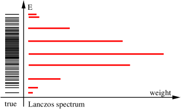
Figure 1: Schematic representation of the approximation of a true energy spectrum by Lanczos energies $\epsilon_{n}$ and their weights $w_{n}(r)=|\langle\,{n(r)}\,|\,{r}\,\rangle|^{2}$, compare Eq. (7).

Effectively, the method provides a coarse grained coverage of the density of states by means of energy representatives $\epsilon_{n}^{(r)}$ that come together with weight factors $w_{n}(r)=|\langle\,{n(r)}\,|\,{r}\,\rangle|^{2}$, thus emulating the true density of levels in the vicinity of the energy representative. In this respect the method has got some similarities to the classical Wang-Landau sampling Wang and Landau (2001); Zhou et al. (2006); Torbrügge and Schnack (2007).

Approximations of the type discussed here essentially suffer from two sources of error: (i) the choice of random vectors in a Hilbert space of large but finite dimension and (ii) the expansion of the exponential in the respective Krylov spaces grown from the random vectors. The error due to choosing a single random vector is upper bounded by ${\cal O}(1/\sqrt{Z_{\text{eff}}})$. In addition, one can prove minimal numbers $R$ of random vectors if a certain minimal probability $(1-\delta)$ is required to stay below a certain relative deviation $\varepsilon$ Roosta-Khorasani and Ascher (2015)

$$\text{Pr}\left(|\text{tr}_{D}^{R}(\!\hbox{}\mathop{\vphantom{A}\smash{A}}\limits_{\sim}\hbox{}\!)-\text{tr}(\!\hbox{}\mathop{\vphantom{A}\smash{A}}\limits_{\sim}\hbox{}\!)|\leq\varepsilon\ \text{tr}(\!\hbox{}\mathop{\vphantom{A}\smash{A}}\limits_{\sim}\hbox{}\!)\right)\geq 1-\delta\ .$$ (8)

Here $\text{tr}_{D}^{R}(\!\hbox{}\mathop{\vphantom{A}\smash{A}}\limits_{\sim}\hbox{}\!)$ denotes a trace with respect to a mathematical distribution $D$ of random numbers, that is averaged over $R$ realizations. For the Hutchinson method one obtains $R\geq 6\varepsilon^{-2}\text{ln}(2/\delta)$, for a Gaussian distribution $R\geq 8\varepsilon^{-2}\text{ln}(2/\delta)$ Roosta-Khorasani and Ascher (2015).

The error related to the specific approximation of the exponential, e.g. Krylov or Chebyshev, is not so simple to quantify, which is one of the reasons for our numerical study. The central question is how accurate the coarse grained Lanczos spectrum represents the true spectrum in the partition function for various temperatures. It is evident from the schematic representation given in Fig. 1 that the Lanczos spectrum does not provide accurate resonance frequencies for more than the lowest energy gaps, even if these are indeed very accurate thanks to the (in $N_{L}$) exponentially fast convergence of extremal eigenvalues in the Lanczos method Saad (1980). In addition, symmetries of the Hamiltonian can not only be used to yield smaller orthogonal subspaces ${\mathcal{H}}(\gamma)$ according to Eq. (7) which helps to access larger system sizes and/or to make calculations faster and less memory consuming, but also to generate a larger number of very accurate Lanczos energy values since they are extremal in their respective subspaces. However, even if the lowest Lanczos energies are very accurate, this does not automatically imply that the related weights $w_{n}(r)$ share the same superb accuracy. The low-temperature behavior thus remains to be further explored. Only at $T=0$ the observables are bound to be correct as long as the the random vector has got some overlap with the true (non-degenerate) ground state Pavarini et al. (2017); Balz et al. (2018). One the other hand, for high temperatures one can show that the expansion of the exponential in Krylov space up to order $N_{L}$ corresponds to a high-temperature series expansion of equilibrium expectation values up to the same order Pavarini et al. (2017). Overall, relation (3) could be derived in Ref. Pavarini et al. (2017) under rather reasonable assumptions. This relation will be our reference in the upcoming part of the paper.

In the following we estimate the uncertainty of a physical quantity approximated by a trace estimator by repeating the numerical evaluation $N_{S}$ times. The generated set of results is considered as a statistical sample, for which we define the standard deviation of the observable in the following way:

$$\delta(O) = \sqrt{\frac{1}{N_{S}}\sum_{r=1}^{N_{S}}\;\left(O^{\text{m}}(T,B)\right)^{2}-\left(\frac{1}{N_{S}}\sum_{r=1}^{N_{S}}\;O^{\text{m}}(T,B)\right)^{2}}$$ (9)

$$= \sqrt{\overline{\left(O^{\text{m}}(T,B)\right)^{2}}-\left(\overline{O^{\text{m}}(T,B)}\right)^{2}}\ .$$

$O^{\text{m}}(T,B)$ is either evaluated according to Eq. (4) or to Eq. (6), depending on whether the fluctuations of approximations with respect to one random vector or with respect to an average over $R$ vectors shall be investigated (cf. the following examples).

In the following numerical examples two observables are considered, zero-field susceptibility and heat capacity. Both are evaluated as variances of magnetization and energy, respectively, i.e.

$$\chi(T) = \frac{(g\mu_{B})^{2}}{k_{B}T}\,\Bigg{\{}\left\langle(\!\hbox{}\mathop{\vphantom{S}\smash{S}}\limits_{\sim}\!{}^{z})^{2}\right\rangle-\left\langle\!\hbox{}\mathop{\vphantom{S}\smash{S}}\limits_{\sim}\!{}^{z}\right\rangle^{2}\Bigg{\}}$$ (10)

$$C(T) = \frac{k_{B}}{(k_{B}T)^{2}}\,\Bigg{\{}\left\langle\!\hbox{}\mathop{\vphantom{H}\smash{H}}\limits_{\sim}\!{}^{2}\right\rangle-\left\langle\!\hbox{}\mathop{\vphantom{H}\smash{H}}\limits_{\sim}\hbox{}\!\right\rangle^{2}\Bigg{\}}\ .$$ (11)

III Numerical results

In this section we investigate various spin systems. They are of finite size and modeled by Heisenberg Hamiltonians augmented with a Zeeman term, i.e.

$$\!\hbox{}\mathop{\vphantom{H}\smash{H}}\limits_{\sim}\hbox{}\! = -2\;\sum_{i<j}\;J_{ij}\!\hbox{}\mathop{\vphantom{\vec{s}}\smash{\vec{s}}}\limits_{\sim}\!{}_{i}\cdot\!\hbox{}\mathop{\vphantom{\vec{s}}\smash{\vec{s}}}\limits_{\sim}\!{}_{j}+g\mu_{B}\,B\,\sum_{i}\;\!\hbox{}\mathop{\vphantom{s}\smash{s}}\limits_{\sim}\!{}^{z}_{i}\ ,$$ (12)

where the first sum runs over ordered pairs of spins (“$-2J$” convention used). Our original intention was to identify systems and circumstances where the approach of Eq. (6) fails. But none of the investigated systems turned out to be (systematically) intractable.

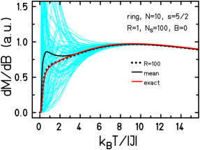
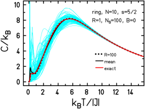
Figure 2: Spin ring $N=10$, $s=5/2$: The light-blue curves depict 100 different estimates of the differential susceptibility as well as the heat capacity using single vectors. Mean values as well as the exact result are also presented.

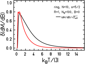
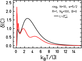
Figure 3: Spin ring $N=10$, $s=5/2$: Standard deviation (red) of the differential susceptibility as well as the heat capacity compared to the error estimate (black).

III.1 Spin ring

As a first example we examine a spin ring with $N=10$ spins $s=5/2$ and nearest-neighbor antiferromagnetic interaction. This system exists as a magnetic molecule (abbreviated Fe₁₀), and it is called a “ferric wheel” Taft et al. (1994). Although the dimension of the total Hilbert space is 60,466,176, the Heisenberg Hamiltonian can be diagonalized completely thanks to the high symmetry (SU(2) and C₁₀) Schnalle and Schnack (2010).

Figure 2 shows $N_{S}=100$ calculations of the differential susceptibility as well as the heat capacity according to Eq. (4), i.e. using a single random vector for each estimate together with the means according to Eqs. (5) and (6). For the calculation $\!\hbox{}\mathop{\vphantom{S}\smash{S}}\limits_{\sim}\!{}^{z}$-symmetry was employed. In addition the exact result is depicted. One can clearly see that the estimates using a single random vector fluctuate largely for temperatures less than ten times the coupling. Nevertheless, if the estimates are joined in an FTLM fashion according to Eq. (6), the result for $R=100$ can be hardly distinguished from the exact calculation. A simple mean according to Eq. (5) fails.

A statistical analysis of the set of estimates $O^{\text{r}}(T,B)$ in Fig. 3 reveals that the error estimate (3) with $\alpha=1$ indeed accurately describes the standard deviation. Only for temperatures smaller than the exchange coupling larger deviations can be observed, but they do not exceed the error estimate much (e.g. by orders of magnitude).

III.2 Cuboctahedron & Icosidodecahedron

As a second example we choose two frustrated polytopes: the cuboctahedron as well as the icosidodecahedron with antiferromagnetic nearest-neighbor interactions. Not only do both exist as magnetic molecules Müller et al. (1999, 2001); Botar et al. (2005); Todea et al. (2007); Schröder et al. (2008); Todea et al. (2009); Palacios et al. (2016), they are also itimately related to the kagomé lattice antiferromagnet Rousochatzakis et al. (2008); Schmidt et al. (2017); Schnack (2019). In contrast to the bipartite spin ring discussed above, these spin systems possess a rather dense spectrum with for instance several to many singlet states below the first triplet state (a hallmark of geometric frustration).

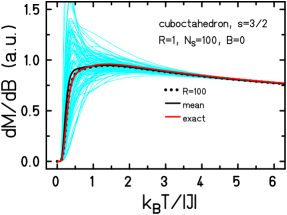
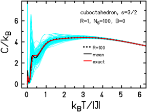
Figure 4: Cuboctahedron $N=12$, $s=3/2$: The light-blue curves depict 100 different estimates ($R=1$) of the differential susceptibility as well as the heat capacity. Mean values as well as the exact result are also presented.

For the cuboctahedron, that has 12 spin sites, we choose a single-spin quantum number of $s=3/2$ since we can still completely diagonalize the Hamiltonian using symmetries although the dimension of the total Hilbert space is 16.777.216 Schnack and Schnalle (2009). As can be seen in Fig. 4, the magnetic observables fluctuate below a temperature of five times the coupling when evaluated with respect to a single random vector. Aggregating them into an FTLM estimate with $R=100$ again yields a very good approximation compared to the exact result.

Since the system is not too big we repeated this analysis for $N_{S}=100$ samples of FTLM estimates with $R=100$ each (in this case $O^{\text{m}}(T,B)$ of Eq. (9) equals $O^{\text{FTLM}}(T,B)$ of Eq. (6)). The result is shown in Fig. 5. One immediately recognizes the much smaller spread of the estimates. Only at (sharp) features of the respective functions deviations are still visible. The origin can be found in strong variations of the true density of states with energy and/or external magnetic field; such variations seem to be hard to emulate by the coarse grained coverage through the trace estimator. The related standard deviations are expected to further decrease in a Monte-Carlo-fashion by a factor of $1/\sqrt{R}$, compare Pavarini et al. (2017). This is indeed found as depicted in Fig. 6. The solid curves display the true standard deviation as well as the estimate for $R=1$, whereas the dashed curves do the same but for $R=100$. Since $\sqrt{100}=10$, the fluctuations of the trace estimator should be ten times smaller, which agrees with the numerical study.

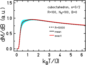
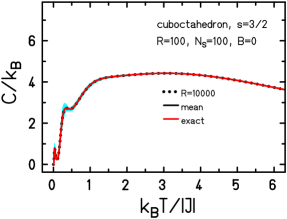
Figure 5: Cuboctahedron $N=12$, $s=3/2$: The light-blue curves depict 100 different estimates ($R=100$) of the differential susceptibility as well as the heat capacity. Mean values as well as the exact result are also presented.

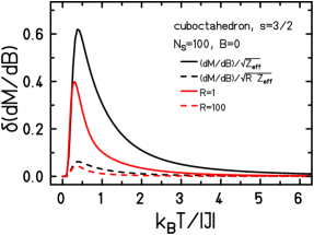
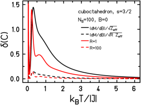
Figure 6: Cuboctahedron $N=12$, $s=3/2$: Standard deviation of the differential susceptibility as well as the heat capacity compared to the error estimate for two sets of estimates, one with $R=1$ (solid curves) and one with $R=100$ (dashed curves).

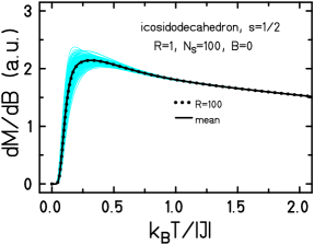
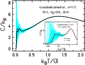
Figure 7: Icosidodecahedron $N=30$, $s=1/2$: The light-blue curves depict 100 different estimates of the differential susceptibility as well as the heat capacity. Mean values are also presented.

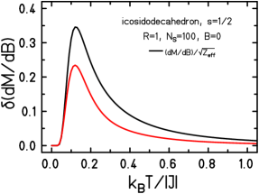
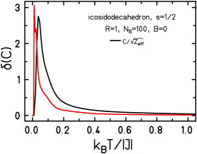
Figure 8: Icosidodecahedron $N=30$, $s=1/2$: Standard deviation (red) of the differential susceptibility as well as the heat capacity compared to the error estimate (black).

The icosidodecahedron – a keplerate molecule – could be synthesized with various ions leading to single spin quntum numbers of $s=1/2$ Botar et al. (2005); Todea et al. (2009), $s=3/2$ Todea et al. (2007); Schröder et al. (2008), and $s=5/2$ Müller et al. (1999, 2001). Only the spin-1/2-version can be calculated by means of trace estimators (typicallity methods) since the dimension of the total Hilbert space is 1,073,741,824. For $s=1$ it would already be $\sim 2\cdot 10^{14}$ and thus out of reach for such methods.

The spectrum of the icosidodecahedron features similar properties as that of the cuboctahedron or that of finite-size realizations of the kagomé lattice Schmidt et al. (2005); Rousochatzakis et al. (2008); Schnack et al. (2018): the spectrum is rather dense, which in particular means that many singlets populate the energy spectrum below the lowest triplet level. The latter has a stark impact on the low-temperature behavior of the heat capacity. On the other hand, for a given temperature a dense spectrum leads to a much larger effective partition function $Z_{\text{eff}}$ in (3) compared to e.g. a bipartite spin system with pronounced low-lying energy gaps and thus to smaller fluctuations at this temperature. Comparing Figs. 2 and 7, one notices that the fluctuations of the estimators were visible below $k_{B}T\approx 10|J|$ for the ferric wheel, whereas this value is only $k_{B}T\approx 1|J|$ for the icosidodecahedron. This means, that a single random vector is sufficient for the evaluation of these observables $k_{B}T\gtrapprox 1|J|$, which constitutes a drastic reduction of the computational effort. One could thus sloppily say that frustration works in favor of trace estimators, cf. Ref. Prelovšek and Kokalj (2018).

The respective standard deviations support these impressions. Only at the lowest temperatures – corresponding to the low-lying level structure in particular of the singlet states – the specific heat estimates express large fluctuations. The susceptibility is not affected, since the low-lying singlets are non-magnetic.

III.3 Delta chain

The above discussed spin systems have a pretty regular (dome-shaped, close to Gaussian) density of states. As our next example we would like to investigate a delta chain (also sawtooth chain) close to the quantum critical point Krivnov et al. (2014); Dmitriev and Krivnov (2015). We choose a chain of $N=32$ sites with a ferromagnetic nearest-neighbor interaction $J_{1}$ and a next-nearest neighbor antiferromagnetic interaction $J_{2}$ between spins on adjacent odd sites, i.e. $i$ and $i+2$ with $i=1,3,5,\dots$. Periodic boundary conditions are applied. At the quantum critical point (QCP), $|J_{2}/J_{1}|=1/2$, the system features a massive degeneracy due to multi-magnon flat bands. Therefore, close to the QCP an additional small energy scale is created, around which the density of states exhibits an additional low-energy maximum. It is worth mentioning that such a compound, that is very close to the QCP, could be synthesized recently Baniodeh et al. (2018).

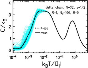
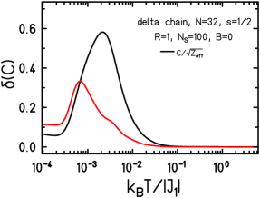
Figure 9: Delta chain $N=32$, $s=1/2$, $|J_{2}/J_{1}|=0.45$: heat capacity, standard deviation and density of states (from top to bottom). The light-blue curves depict 100 different estimates of the heat capacity. Mean values are also presented. The density of states is presented for excited levels with excitation energy $E^{*}$.

When evaluating the estimates one notices that fluctuations of observables appear only for temperatures of the order of the emergent small energy scale, as can be seen in Fig. 9. This energy scale, which is approximately $10^{-2}|J_{1}|$ and corresponds to the low-temperature maximum, is much smaller than the dominant scale $|J_{1}|$, that corresponds to the high-temperature Shottky peak.

The reason for this behavior can be traced back to the enormous number of low-lying levels assembled at the low-energy scale, compare density of states in Fig. 9, that at temperatures elevated above the low-temperature scale contribute to the effective partition function (3) and thus lead to a very small estimate for the fluctuations of any observable. This is clearly seen for $\delta(C)$ in Fig. 9, which virtually drops to zero above the low-temperature scale. Also in this case a single random vector suffices to evaluate the thermal behavior above the low-temperature scale.

III.4 An integrable spin system

We already mentioned that the use of the concept of typicality for trace estimators is not connected to the question whether ETH holds for the respective system or not. Here we present a simple example of a spin-1/2 chain with nearest-neighbor antiferromagnetic interaction, that would be integrable via the Bethe ansatz Bethe (1931); Kulish et al. (1981); Takhtajan (1982); Babujian (1983). We investigate a spin chain of $N=24$ spins $s=1/2$ with periodic boundary conditions that can also be solved numerically exactly when employing the symmetry groups SU(2) and C_N Heitmann and Schnack (2019). For the FTLM investigation a reduced symmetry was used, namely $\!\hbox{}\mathop{\vphantom{S^{z}}\smash{S^{z}}}\limits_{\sim}\hbox{}\!$–symmetry as well as translational symmetry C_N.

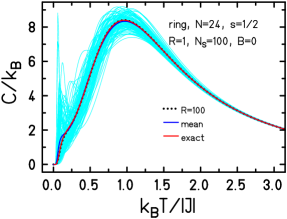
Figure 10: Spin ring $N=24$, $s=1/2$: The light-blue curves depict 100 different estimates of the heat capacity. Mean values as well as the exact result are also presented.

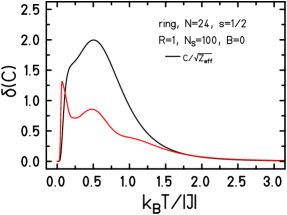
Figure 11: Spin ring $N=24$, $s=1/2$: Standard deviation (red) of the heat capacity compared to the error estimate (black).

In Figs. 10 and 11 we present our results for the heat capacity. The susceptibilty (not shown) behaves similarly. The results are very similar to the already discussed examples. The largest deviations again occur at and below a temperature scale of the order of the exchange interaction $|J|$. A sharp peak of the standard deviation $\delta(C)$ at very low temperatures occurs at temperatures coressponding to the lowest (singlet-triplet) gap. However, one would expect for this class of spin systems that the temperature above which the approximation is good drops with increasing system size since the lowest gaps shrink for this system that is gapless in the thermodynamic limit.

III.5 A Haldane spin system

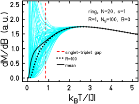
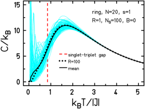
Figure 12: Spin ring $N=20$, $s=1$: The light-blue curves depict 100 different estimates of the differential susceptibility as well as the heat capacity. Mean values as well as the exact result are also presented.

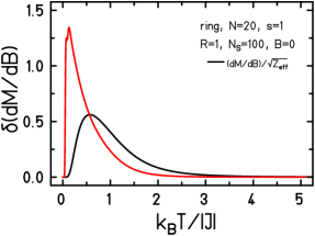
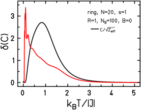
Figure 13: Spin ring $N=20$, $s=1$: Standard deviation (red) of the differential susceptibility as well as the heat capacity compared to the error estimate (black).

The question how the lowest gap influences the low temperature quality of the approximation will be addressed in this section. To this end we choose a Haldane spin chain of $N=20$ and $s=1$ with nearest neighbor antiferromagnetic exchange as an example for systems where the lowest gap is sizable and does not even close in the thermodynamic limit.

As one can see in Fig. 12 both susceptibility as well as heat capacity fluctuate largely about and below a temperature scale that is provided by the lowest energy gap (dashed vertical line). In essence this means – here and for all previous examples – that a single random vector, Eq. (4), does not work for temperatures of this order and below, except for $T=0$ where the method is bound to be exact Jaklič and Prelovšek (2000); Pavarini et al. (2017). This is also clearly reflected by the respective standard deviations shown in Fig. 13. In addition, here we encounter an example where the standard deviation $\delta(\text{d}\mathcal{M}/\text{d}B)$ assumes values much larger than our estimator (3) for $T>0$.

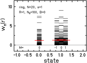
Figure 14: Spin ring $N=20$, $s=1$: Weights $w_{n}(r)$ of the ground state singlet and the first excited triplet (black bars). Mean weigths are depicted by thick red bars. Technically, the weights for $M=-1$ are a simple copy of those for $M=+1$ thanks to symmetry.

The reason of the strong fluctuations of low-temperature observables lies in a poor coverage of $w_{n}(r)$ for the lowest energy eigenvalues. Although the lowest eigenvalues, thanks to the properties of power methods, are very accurate, i.e. possess a standard deviation of $<10^{-4}$ or better, the corresponding weight factors fluctuate largely. This can be seen in Fig. 14 where the weigths $w_{n}(r)$ are displayed for the ground state and the first excited state as they are evaluated in the respective Hilbert subspaces $\mathcal{H}\left(M\right)$. These fluctuations of the weights are conserved by a power method, this is particularily important for the low-lying levels. In order to yield an accurate low-temperature partition function the weights of the lowest states should equal one in (7). The naturally occuring variation of the weights in a random vector are amplified at low temperature by the Boltzmann factor. One can derive an estimate for the relative error of the specific heat assuming (for simplicity) that at low temperatures only the ground state as well as the first excited state contribute to the partition function,

$$\frac{\delta(C)}{C} \approx \left|\frac{\frac{w_{1}}{w_{0}}(1+d\exp[-\beta\Delta])^{2}}{(1+\frac{w_{1}}{w_{0}}d\exp[-\beta\Delta])^{2}}-1\right|$$ (13)

$$\rightarrow \left|\frac{w_{1}}{w_{0}}-1\right|\ ,\ \text{for}\ \beta\rightarrow\infty\ .$$ (14)

Here $\Delta$ is the gap between ground and first excited state, $d$ the degeneracy of the first excited state, and $w_{0}$ and $w_{1}$ the weights of the ground and the first excited state. The ratio of both dominates the relative error at low temperatures; it can assume large values. This problem is independent of the observable at hand, it stems from the fluctuations that are intrinsic to the random vector. Therefore, Eq. (14) does not only hold for the heat capacity, which is a variance $\left\langle\!\hbox{}\mathop{\vphantom{H}\smash{H}}\limits_{\sim}\!{}^{2}\right\rangle-\left\langle\!\hbox{}\mathop{\vphantom{H}\smash{H}}\limits_{\sim}\hbox{}\!\right\rangle^{2}$, but for $\left\langle\!\hbox{}\mathop{\vphantom{H}\smash{H}}\limits_{\sim}\!{}^{2}\right\rangle$ and $\left\langle\!\hbox{}\mathop{\vphantom{H}\smash{H}}\limits_{\sim}\hbox{}\!\right\rangle$ separately.

Although every random vector possesses these fluctuations, a proper averaging as outlined in (7) decreases the fluctuations drastically. Figure 14 demonstrates that after averaging over 100 random vectors, the averaged weights (thick red bars) approach an equal magnitude although not yet one, but $\sim 1.2$. For most observables it is sufficient that the averaged weights of the lowest states are about the same since they appear simultaneously in numerator and denominator of Eq. (6). Quite recently new ideas have been formulated how to improve the low-temperature estimates of FTLM also for small numbers $R$ of random vectors by taking special care of the weights for low-lying levels Morita and Tohyama (2019).

The investigation of the averaged weights of low-lying levels also sheds light on the failure of the naive mean according to Eq. (5). This kind of a mean does not average the individual weights, but the individual single-vector expectation values, which converges either very slowly or even to a different function at low temperatures.

IV Discussion and conclusions

Finally, we can conclude that typicality-based methods allow an astonishingly accurate approximation of static thermodynamics observables sometimes using just one random vector. This qualifies methods such as FTLM for a reliable treatment of large quantum systems, in particular of those that cannot be delt with by quantum Monte Carlo due to the sign prolem and of those where approximations using matrix product states converge slowly such as the two-dimensional kagomé lattice Schnack et al. (2018).

The simple idea of typicality to replace a trace by an expectation value with respect to just one random vector works indeed for large enough temperatures. $1/\sqrt{Z_{\text{eff}}}$ provides the estimate for the relative error to be expected for temperatures well above the lowest excitation gap. An additional average over many random vectors according to (6) further increases the accurcy in a Monte-Carlo fashion and reduces the error by another factor $1/\sqrt{R}$, where $R$ is the number of employed random vectors. The simple average (5) of single-vector approximations does not converge properly especially at low temperatures.

Although power methods such as the Lanczos method yield exact ground state expectation values for systems with non-degenerate ground states, and should thus be accurate at $T=0$, the large fluctuations of estimates using a single random vector surprise. We could clarify the latter problem by elucidating the important role jointly played by the energy gap between ground state and first excited state as well as the weight factors of both states. Although both energies are spectroscopically accurate it needs sufficient averaging to tame the strongly fluctuating weight factors. In view of this, and with $1/\sqrt{Z_{\text{eff}}}$ in mind, one can state that the discussed approximations work better for systems with small gap and larger density of low-lying states. Therefore, frustration works in favor of trace estimators.

Overall, we conclude that methods such as FTLM, which rely on trace estimators, are astonishingly accurate. We could demonstrate with several prototypical examples that the standard deviations of observables can be systematically reduced via averaging. In addition, we are convinced that we could provide a valuable contribution in order to trust these methods by presenting realistic standard deviations The Editors (2011).

References

- Skilling (1988) J. Skilling, “Maximum Entropy and Bayesian Methods,” (Kluwer, Dordrecht, 1988) Chap. The eigenvalues of mega-dimensional matrices, pp. 455–466.
- Hutchinson (1989) M. Hutchinson, “A Stochastic Estimator of the Trace of the Influence Matrix for Laplacian Smoothing Splines,” Communications in Statistics - Simulation and Computation 18, 1059 (1989).
- Drabold and Sankey (1993) D. A. Drabold and O. F. Sankey, “Maximum entropy approach for linear scaling in the electronic structure problem,” Phys. Rev. Lett. 70, 3631 (1993).
- Jaklič and Prelovšek (1994) J. Jaklič and P. Prelovšek, “Lanczos method for the calculation of finite-temperature quantities in correlated systems,” Phys. Rev. B 49, 5065 (1994).
- Silver and Röder (1994) R. N. Silver and H. Röder, “Densities of states of mega-dimensional Hamiltonian matrices,” Int. J. Mod. Phys. C 5, 735 (1994).
- Golub and von Matt (1997) G. H. Golub and U. von Matt, Tikhonov Regularization for Large Scale Problems, Tech. Rep. (Stanford University, 1997) technical report SCCM-97-03.
- Weiße et al. (2006) A. Weiße, G. Wellein, A. Alvermann, and H. Fehske, “The kernel polynomial method,” Rev. Mod. Phys. 78, 275 (2006).
- Avron and Toledo (2011) H. Avron and S. Toledo, “Randomized Algorithms for Estimating the Trace of an Implicit Symmetric Positive Semi-definite Matrix,” J. ACM 58, 8:1 (2011).
- Roosta-Khorasani and Ascher (2015) F. Roosta-Khorasani and U. Ascher, “Improved Bounds on Sample Size for Implicit Matrix Trace Estimators,” Found. Comput. Math. 15, 1187 (2015).
- Saibaba et al. (2017) A. K. Saibaba, A. Alexanderian, and I. C. F. Ipsen, “Randomized matrix-free trace and log-determinant estimators,” Numer. Math. 137, 353 (2017).
- Collins and Śniady (2006) B. Collins and P. Śniady, “Integration with Respect to the Haar Measure on Unitary, Orthogonal and Symplectic Group,” Commun. Math. Phys. 264, 773 (2006).
- Bartsch and Gemmer (2009) C. Bartsch and J. Gemmer, “Dynamical Typicality of Quantum Expectation Values,” Phys. Rev. Lett. 102, 110403 (2009).
- Reimann (2016) P. Reimann, “Typical fast thermalization processes in closed many-body systems,” Nature Communications 7, 10821 (2016).
- Deutsch (1991) J. M. Deutsch, “Quantum statistical mechanics in a closed system,” Phys. Rev. A 43, 2046 (1991).
- Srednicki (1994) M. Srednicki, “Chaos and quantum thermalization,” Phys. Rev. E 50, 888 (1994).
- Rigol et al. (2008) M. Rigol, V. Dunjko, and M. Olshanii, “Thermalization and its mechanism for generic isolated quantum systems,” Nature 452, 854 (2008).
- D’Alessio et al. (2016) L. D’Alessio, Y. Kafri, A. Polkovnikov, and M. Rigol, “From quantum chaos and eigenstate thermalization to statistical mechanics and thermodynamics,” Adv. Phys. 65, 239 (2016).
- Borgonovi et al. (2016) F. Borgonovi, F. M. Izrailev, L. F. Santos, and V. G. Zelevinsky, “Quantum chaos and thermalization in isolated systems of interacting particles,” Phys. Rep. 626, 1 (2016).
- Nandkishore and Huse (2015) R. Nandkishore and D. A. Huse, “Many-Body Localization and Thermalization in Quantum Statistical Mechanics,” Annu. Rev. Condens. Matter Phys. 6, 15 (2015).
- Abanin et al. (2019) D. A. Abanin, E. Altman, I. Bloch, and M. Serbyn, “Colloquium: Many-body localization, thermalization, and entanglement,” Rev. Mod. Phys. 91, 021001 (2019).
- Inoue et al. (2019) K. Inoue, Y. Maeda, H. Nakano, and Y. Fukumoto, “Canonical-Ensemble Calculations of the Magnetic Susceptibility for a Spin-1/2 Spherical Kagome Cluster With Dzyaloshinskii-Moriya Interactions by Using Microcanonical Thermal Pure Quantum States,” IEEE Transactions on Magnetics 55, 1 (2019).
- Sugiura and Shimizu (2012) S. Sugiura and A. Shimizu, “Thermal Pure Quantum States at Finite Temperature,” Phys. Rev. Lett. 108, 240401 (2012).
- Sugiura and Shimizu (2013) S. Sugiura and A. Shimizu, “Canonical Thermal Pure Quantum State,” Phys. Rev. Lett. 111, 010401 (2013).
- Okamoto et al. (2018) S. Okamoto, G. Alvarez, E. Dagotto, and T. Tohyama, “Accuracy of the microcanonical Lanczos method to compute real-frequency dynamical spectral functions of quantum models at finite temperatures,” Phys. Rev. E 97, 043308 (2018).
- Alben et al. (1975) R. Alben, M. Blume, H. Krakauer, and L. Schwartz, “Exact results for a three-dimensional alloy with site diagonal disorder: comparison with the coherent potential approximation,” Phys. Rev. B 12, 4090 (1975).
- De Raedt and de Vries (1989) H. De Raedt and P. de Vries, “Simulation of two and three-dimensional disordered systems: Lifshitz tails and localization properties,” Z. Phys. B Condens. Matter 77, 243 (1989).
- de Vries and De Raedt (1993) P. de Vries and H. De Raedt, “Solution of the time-dependent Schrödinger equation for two-dimensional spin-1/2 Heisenberg systems,” Phys. Rev. B 47, 7929 (1993).
- Dagotto (1994) E. Dagotto, “Correlated electrons in high-temperature superconductors,” Rev. Mod. Phys. 66, 763 (1994).
- Jaklič and Prelovšek (2000) J. Jaklič and P. Prelovšek, “Finite-temperature properties of doped antiferromagnets,” Adv. Phys. 49, 1 (2000).
- Aichhorn et al. (2003) M. Aichhorn, M. Daghofer, H. G. Evertz, and W. von der Linden, “Low-temperature Lanczos method for strongly correlated systems,” Phys. Rev. B 67, 161103(R) (2003).
- Zerec et al. (2006) I. Zerec, B. Schmidt, and P. Thalmeier, “Kondo lattice model studied with the finite temperature Lanczos method,” Phys. Rev. B 73, 245108 (2006).
- Schnack and Wendland (2010) J. Schnack and O. Wendland, “Properties of highly frustrated magnetic molecules studied by the finite-temperature Lanczos method,” Eur. Phys. J. B 78, 535 (2010).
- Prelovšek and Bonča (2013) P. Prelovšek and J. Bonča, “Strongly Correlated Systems, Numerical Methods,” (Springer, Berlin, Heidelberg, 2013) Chap. Ground State and Finite Temperature Lanczos Methods.
- Ummethum et al. (2013) J. Ummethum, J. Schnack, and A. Laeuchli, “Large-scale numerical investigations of the antiferromagnetic Heisenberg icosidodecahedron,” J. Magn. Magn. Mater. 327, 103 (2013).
- Hanebaum and Schnack (2014) O. Hanebaum and J. Schnack, “Advanced finite-temperature Lanczos method for anisotropic spin systems,” Eur. Phys. J. B 87, 194 (2014).
- Psaroudaki et al. (2014) C. Psaroudaki, J. Herbrych, J. Karadamoglou, P. Prelovšek, X. Zotos, and N. Papanicolaou, “Effective description of the chain with strong easy-plane anisotropy,” Phys. Rev. B 89, 224418 (2014).
- Steinigeweg et al. (2015) R. Steinigeweg, J. Gemmer, and W. Brenig, “Spin and energy currents in integrable and nonintegrable spin- chains: A typicality approach to real-time autocorrelations,” Phys. Rev. B 91, 104404 (2015).
- Steinigeweg et al. (2016) R. Steinigeweg, J. Herbrych, F. Pollmann, and W. Brenig, “Typicality approach to the optical conductivity in thermal and many-body localized phases,” Phys. Rev. B 94, 180401(R) (2016).
- Schmidt and Thalmeier (2017) B. Schmidt and P. Thalmeier, “Frustrated two dimensional quantum magnets,” Phys. Rep. 703, 1 (2017).
- Schnack et al. (2018) J. Schnack, J. Schulenburg, and J. Richter, “Magnetism of the kagome lattice antiferromagnet,” Phys. Rev. B 98, 094423 (2018).
- Prelovšek and Kokalj (2018) P. Prelovšek and J. Kokalj, “Finite-temperature properties of the extended Heisenberg model on a triangular lattice,” Phys. Rev. B 98, 035107 (2018).
- Dmitriev et al. (2019) D. V. Dmitriev, V. Y. Krivnov, J. Richter, and J. Schnack, “Thermodynamics of a delta chain with ferromagnetic and antiferromagnetic interactions,” Phys. Rev. B 99, 094410 (2019).
- Richter and Steinigeweg (2019) J. Richter and R. Steinigeweg, “Combining dynamical quantum typicality and numerical linked cluster expansions,” Phys. Rev. B 99, 094419 (2019).
- Rousochatzakis et al. (2019) I. Rousochatzakis, S. Kourtis, J. Knolle, R. Moessner, and N. B. Perkins, “Quantum spin liquid at finite temperature: Proximate dynamics and persistent typicality,” Phys. Rev. B 100, 045117 (2019).
- Manthe and Huarte-Larranaga (2001) U. Manthe and F. Huarte-Larranaga, “Partition functions for reaction rate calculations: statistical sampling and MCTDH propagation,” Chem. Phys. Lett. 349, 321 (2001).
- Huarte-Larranaga and Manthe (2002) F. Huarte-Larranaga and U. Manthe, “Vibrational excitation in the transition state: The CH4 + H CH3 + H2 reaction rate constant in an extended temperature interval,” J. Chem. Phys. 116, 2863 (2002).
- Pavarini et al. (2017) E. Pavarini, E. Koch, R. Scalettar, and R. M. Martin, eds., “The Physics of Correlated Insulators, Metals, and Superconductors,” (2017) Chap. The Finite Temperature Lanczos Method and its Applications by P. Prelovšek, ISBN 978-3-95806-224-5, http://hdl.handle.net/2128/15283.
- Hams and De Raedt (2000) A. Hams and H. De Raedt, “Fast algorithm for finding the eigenvalue distribution of very large matrices,” Phys. Rev. E 62, 4365 (2000).
- Iitaka and Ebisuzaki (2003) T. Iitaka and T. Ebisuzaki, “Algorithm for Linear Response Functions at Finite Temperatures: Application to ESR Spectrum of Antiferromagnet Cu Benzoate,” Phys. Rev. Lett. 90, 047203 (2003).
- Lin et al. (2013) L. Lin, Y. Saad, and C. Yang, “Approximating spectral densities of large matrices,” ArXiv e-prints (2013), arXiv:1308.5467 [math.NA] .
- Wietek et al. (2019) A. Wietek, P. Corboz, S. Wessel, B. Normand, F. Mila, and A. Honecker, “Thermodynamic properties of the Shastry-Sutherland model throughout the dimer-product phase,” Phys. Rev. Research 1, 033038 (2019).
- Monnai and Sugita (2014) T. Monnai and A. Sugita, “Typical Pure States and Nonequilibrium Processes in Quantum Many-Body Systems,” J. Phys. Soc. Jpn. 83, 094001 (2014).
- Iitaka and Ebisuzaki (2004) T. Iitaka and T. Ebisuzaki, “Random phase vector for calculating the trace of a large matrix,” Phys. Rev. E 69, 057701 (2004).
- Steinigeweg et al. (2014) R. Steinigeweg, J. Gemmer, and W. Brenig, “Spin-current autocorrelations from single pure-state propagation,” Phys. Rev. Lett. 112, 120601 (2014).
- Elsayed and Fine (2013) T. A. Elsayed and B. V. Fine, “Regression Relation for Pure Quantum States and Its Implications for Efficient Computing,” Phys. Rev. Lett. 110, 070404 (2013).
- Gemmer et al. (2009) J. Gemmer, M. Michel, and G. Mahler, Quantum Thermodynamics: Emergence of Thermodynamic Behavior Within Composite Quantum Systems, Lecture Notes in Physics, Vol. 784 (Springer, Berlin, Heidelberg, 2009).
- Balz et al. (2018) B. N. Balz, J. Richter, J. Gemmer, R. Steinigeweg, and P. Reimann, “Dynamical Typicality for Initial States with a Preset Measurement Statistics of Several Commuting Observables,” in Thermodynamics in the Quantum Regime: Fundamental Aspects and New Directions, edited by F. Binder, L. A. Correa, C. Gogolin, J. Anders, and G. Adesso (Springer, Cham, 2018) pp. 413–433.
- Reimann and Gemmer (2019) P. Reimann and J. Gemmer, “Why are macroscopic experiments reproducible? Imitating the behavior of an ensemble by single pure states,” Physica A: Statistical Mechanics and its Applications , 121840 (2019).
- Schulenburg (2017) J. Schulenburg, spinpack 2.56, Magdeburg University (2017).
- Richter and Schulenburg (2010) J. Richter and J. Schulenburg, “The spin-1/2 - Heisenberg antiferromagnet on the square lattice: Exact diagonalization for N=40 spins,” Eur. Phys. J. B 73, 117 (2010).
- Wang and Landau (2001) F. Wang and D. P. Landau, “Efficient, Multiple-Range Random Walk Algorithm to Calculate the Density of States,” Phys. Rev. Lett. 86, 2050 (2001).
- Zhou et al. (2006) C. G. Zhou, T. C. Schulthess, S. Torbrügge, and D. P. Landau, “Wang-Landau algorithm for continuous models and joint density of states,” Phys. Rev. Lett. 96, 120201 (2006).
- Torbrügge and Schnack (2007) S. Torbrügge and J. Schnack, “Sampling the two-dimensional density of states of a giant magnetic molecule using the Wang-Landau method,” Phys. Rev. B 75, 054403 (2007).
- Saad (1980) Y. Saad, “On the Rates of Convergence of the Lanczos and the Block-Lanczos Methods,” SIAM Journal on Numerical Analysis 17, 687 (1980).
- Taft et al. (1994) K. L. Taft, C. D. Delfs, G. C. Papaefthymiou, S. Foner, D. Gatteschi, and S. J. Lippard, “[Fe(OMe)2(O2CCH2Cl)]10, a molecular ferric wheel,” J. Am. Chem. Soc. 116, 823 (1994).
- Schnalle and Schnack (2010) R. Schnalle and J. Schnack, “Calculating the energy spectra of magnetic molecules: application of real- and spin-space symmetries,” Int. Rev. Phys. Chem. 29, 403 (2010).
- Müller et al. (1999) A. Müller, S. Sarkar, S. Q. N. Shah, H. Bögge, M. Schmidtmann, S. Sarkar, P. Kögerler, B. Hauptfleisch, A. Trautwein, and V. Schünemann, “Archimedean synthesis and magic numbers: “Sizing” giant molybdenum-oxide-based molecular spheres of the Keplerate type,” Angew. Chem. Int. Ed. 38, 3238 (1999).
- Müller et al. (2001) A. Müller, M. Luban, C. Schröder, R. Modler, P. Kögerler, M. Axenovich, J. Schnack, P. C. Canfield, S. Bud’ko, and N. Harrison, “Classical and quantum magnetism in giant Keplerate magnetic molecules,” ChemPhysChem 2, 517 (2001).
- Botar et al. (2005) B. Botar, P. Kögerler, and C. L. Hill, “[{(Mo)Mo5O21(H2O)3(SO4)}12(VO)30(H2O)20]36-: A molecular quantum spin icosidodecahedron,” Chem. Commun. , 3138 (2005).
- Todea et al. (2007) A. M. Todea, A. Merca, H. Bögge, J. van Slageren, M. Dressel, L. Engelhardt, M. Luban, T. Glaser, M. Henry, and A. Müller, “Extending the {(Mo)Mo5}12M30 Capsule Keplerate Sequence: A {Cr30}–Cluster of Metal Centers with a {Na(H2O)12} Encapsulate,” Angew. Chem. Int. Ed. 46, 6106 (2007).
- Schröder et al. (2008) C. Schröder, R. Prozorov, P. Kögerler, M. D. Vannette, X. Fang, M. Luban, A. Matsuo, K. Kindo, A. Müller, and A. M. Todea, “Multiple nearest-neighbor exchange model for the frustrated magnetic molecules {Mo72Fe30} and {Mo72Cr30},” Phys. Rev. B 77, 224409 (2008).
- Todea et al. (2009) A. M. Todea, A. Merca, H. Bögge, T. Glaser, L. Engelhardt, R. Prozorov, M. Luban, and A. Müller, “Polyoxotungstates now also with pentagonal units: supramolecular chemistry and tuning of magnetic exchange in {(M)M5}12V30 Keplerates (M = Mo, W),” Chem. Commun. , 3351 (2009).
- Palacios et al. (2016) M. A. Palacios, E. M. Pineda, S. Sanz, R. Inglis, M. B. Pitak, S. J. Coles, M. Evangelisti, H. Nojiri, C. Heesing, E. K. Brechin, J. Schnack, and R. E. P. Winpenny, “Copper Keplerates: High Symmetry Magnetic Molecules,” ChemPhysChem 17, 55 (2016).
- Rousochatzakis et al. (2008) I. Rousochatzakis, A. M. Läuchli, and F. Mila, “Highly frustrated magnetic clusters: The kagomé on a sphere,” Phys. Rev. B 77, 094420 (2008).
- Schmidt et al. (2017) H.-J. Schmidt, A. Hauser, A. Lohmann, and J. Richter, “Interpolation between low and high temperatures of the specific heat for spin systems,” Phys. Rev. E 95, 042110 (2017).
- Schnack (2019) J. Schnack, “Large magnetic molecules and what we learn from them,” Contemp. Phys. 60, 127 (2019).
- Schnack and Schnalle (2009) J. Schnack and R. Schnalle, “Frustration effects in antiferromagnetic molecules: the cuboctahedron,” Polyhedron 28, 1620 (2009).
- Schmidt et al. (2005) R. Schmidt, J. Schnack, and J. Richter, “Frustration effects in magnetic molecules,” J. Magn. Magn. Mater. 295, 164 (2005).
- Krivnov et al. (2014) V. Y. Krivnov, D. V. Dmitriev, S. Nishimoto, S.-L. Drechsler, and J. Richter, “Delta chain with ferromagnetic and antiferromagnetic interactions at the critical point,” Phys. Rev. B 90, 014441 (2014).
- Dmitriev and Krivnov (2015) D. V. Dmitriev and V. Y. Krivnov, “Delta chain with anisotropic ferromagnetic and antiferromagnetic interactions,” Phys. Rev. B 92, 184422 (2015).
- Baniodeh et al. (2018) A. Baniodeh, N. Magnani, Y. Lan, G. Buth, C. E. Anson, J. Richter, M. Affronte, J. Schnack, and A. K. Powell, “High spin cycles: topping the spin record for a single molecule verging on quantum criticality,” npj Quantum Materials 3, 10 (2018).
- Bethe (1931) H. Bethe, “Zur Theorie der Metalle,” Z. Phys. 71, 205 (1931).
- Kulish et al. (1981) P. P. Kulish, N. Yu. Reshetikhin, and E. K. Sklyanin, “Yang-Baxter equation and representation theory: I,” Lett. Math. Phys. 5, 393 (1981).
- Takhtajan (1982) L. Takhtajan, “The picture of low-lying excitations in the isotropic Heisenberg chain of arbitrary spins,” Phys. Lett. A 87, 479 (1982).
- Babujian (1983) H. Babujian, “Exact solution of the isotropic Heisenberg chain with arbitrary spins: Thermodynamics of the model,” Nucl. Phys. B 215, 317 (1983).
- Heitmann and Schnack (2019) T. Heitmann and J. Schnack, “Combined use of translational and spin-rotational invariance for spin systems,” Phys. Rev. B 99, 134405 (2019).
- Morita and Tohyama (2019) K. Morita and T. Tohyama, “Finite-temperature properties of the Kitaev-Heisenberg models on kagome and triangular lattices studied by improved finite-temperature Lanczos methods,” ArXiv e-prints (2019), arXiv:1911.09266 [cond-mat.str-el] .
- The Editors (2011) The Editors, “Editorial: Uncertainty Estimates,” Phys. Rev. A 83, 040001 (2011).