Energy momentum tensor and the $D$-term in the bag model

Abstract

The energy-momentum tensor (EMT) form factors pave new ways for exploring hadron structure. Especially the $D$-term related to the EMT form factor $D(t)$ has received a lot of attention due to its attractive physical interpretation in terms of mechanical properties. We study the nucleon EMT form factors and the associated densities in the bag model which we formulate for an arbitrary number of colors $N_{c}$ and show that the EMT form factors are consistently described in this model in the large-$N_{c}$ limit. The simplicity of the model allows us to test in a lucid way many theoretical concepts related to EMT form factors and densities including recently introduced concepts like normal and tangential forces, or monopole and quadrupole contributions to the angular momentum distribution. We also study the $D$-terms of $\rho$-meson, Roper resonance, other $N^{\ast}$ states and $\Delta$-resonances. Among the most interesting outcomes is the lucid demonstration of the deeper connection of EMT conservation, stability, the virial theorem and the negative sign of the $D$-term.

I Introduction

The perspective to access hadronic EMT form factors Kobzarev:1962wt through studies of generalized parton distribution functions (GPDs) Mueller:1998fv in hard exclusive reactions Ji:1996ek ; Radyushkin:1996nd ; Collins:1996fb ; Goeke:2001tz ; Diehl:2003ny and their attractive interpretation in terms of mechanical properties Polyakov:2002yz have attracted lots of interest in recent literature, see the review Polyakov:2018zvc . EMT form factors were studied in models Ji:1997gm ; Petrov:1998kf ; Schweitzer:2002nm ; Ossmann:2004bp ; Wakamatsu:2005vk ; Wakamatsu:2006dy ; Goeke:2007fp ; Goeke:2007fq ; Wakamatsu:2007uc ; Cebulla:2007ei ; Kim:2012ts ; Jung:2013bya ; Jung:2014jja ; Perevalova:2016dln ; Abidin:2008ku ; Abidin:2008hn ; Brodsky:2008pf ; Abidin:2009hr ; Mamo:2019mka ; Megias:2004uj ; Megias:2005fj ; Broniowski:2008hx ; Kumar:2017dbf ; Chakrabarti:2015lba ; Mai:2012yc ; Mai:2012cx ; Cantara:2015sna ; Gulamov:2015fya ; Nugaev:2019vru ; Hudson:2017xug ; Freese:2019bhb ; Freese:2019eww , chiral perturbation theory Belitsky:2002jp ; Ando:2006sk ; Diehl:2006ya , meson-dominance approach Masjuan:2012sk , dispersion relations Pasquini:2014vua , lattice QCD Mathur:1999uf ; Hagler:2003jd ; Hagler:2007xi ; Shanahan:2018pib , QCD lightcone sum rules Anikin:2019kwi and for photons Gabdrakhmanov:2012aa ; Friot:2006mm . Especially the form factor $D(t)$ Polyakov:1999gs ; Teryaev:2001qm gained increased attention due to its interpretation in terms of internal forces Polyakov:2002yz spurred by recent attempts to extract phenomenological information on $D(t)$ Kumano:2017lhr ; Nature ; Kumericki:2019ddg .

In this work we present a study of EMT properties in one of the simplest hadronic models: the bag model Chodos:1974je ; Chodos:1974pn ; DeGrand:1975cf . This model was introduced more than 40 years ago, but is still in use and continues giving helpful contributions to the understanding of hadron structure. In fact, the bag model has been used as an exploratory theoretical framework in many instances, often being the first model (or one of the first models) where newly introduced hadronic properties were investigated, including studies of nucleon structure functions Jaffe:1974nj ; Celenza:1982uk , transversity and other chiral-odd parton distribution functions Jaffe:1991ra , transverse momentum dependent parton distributions Courtoy:2008vi ; Avakian:2008dz ; Avakian:2010br , or double parton distribution functions Chang:2012nw ; Rinaldi:2013vpa . The bag model was also the first model where GPDs and EMT form factors were studied Ji:1997gm .

In the present study we will extend the work of Ref. Ji:1997gm in multiple respects, and investigate within this model concepts which appeared only after Ref. Ji:1997gm . This includes the EMT densities introduced in Polyakov:2002yz and further developed in Polyakov:2018zvc and Lorce:2017wkb ; Schweitzer:2019kkd ; Polyakov:2018guq ; Polyakov:2018exb ; Lorce:2018egm ; Polyakov:2018rew ; Cosyn:2019aio ; Polyakov:2019lbq . The bag model provides an attractive theoretical framework for that. The version of the bag model used in this work is at variance with chiral symmetry which is a drawback. This model has, however, also important advantages: it is a consistent theoretical framework. Its simplicity allows one to obtain lucid insights which are more difficult to deduce from more complex models. Our results will help to improve the understanding of the nucleon structure and the EMT densities. The layout of our study is as follows.

After defining the EMT form factors and densities in Sec. II, we briefly introduce the bag model in Sec. III and study the quark EMT form factors in Sec. IV using a formulation of the model for a large number of colors $N_{c}$. The large-$N_{c}$ limit will allow us to avoid technical problems associated with the evaluation of form factors in so-called independent-particle models like the bag model. We will use the large-$N_{c}$ limit as a tool to derive consistent model expressions, and show that the $1/N_{c}$-corrections to the form factors are relatively small for small momentum transfers. In addition, the large-$N_{c}$ limit provides a rigorous justification for the concept of 3D densities which are studied in detail in Sec. V. We will evaluate the “gluonic” form factor $\bar{c}^{G}(t)$ due to the bag which can only be computed by taking advantage of the EMT density formalism, and we will rigorously prove the internal consistency of the description. The Sec. VI presents an extensive study of the $D$-term for the nucleon and other hadronic states including $N^{\star}$ states, $\rho$-mesons, and the $\Delta$-resonances. We also include an insightful study of hypothetical highly excited bag model states. This is the only study of EMT properties of excited states available in literature besides $Q$-balls Mai:2012cx and we make the interesting observation that in both systems asymptotically the $D$-term grows as $D=-\,{\rm const}\times M^{8/3}$ with the mass $M$ of the excitation, even though the excited states have much different internal structures in the two frameworks. The Sec. VII is dedicated to studies of limiting cases like the heavy quark limit, the large bag-radius limit, and the non-relativistic limit of the nucleon, and discuss the behavior of the $D$-term in these limits. Our study is complemented by an instructive discussion in Sec. VIII of the $D$-term in a predecessor of the bag model Thomas:2001kw , the Bogoliubov model Bogo:1967 , which is a counter-example where the nucleon is not fully consistently described. As a consequence one finds an unphysical (positive) $D$-term in this model. This example also illustrates the necessity to study the complete EMT structure. The conclusions are presented in Sec. IX and technical details can be found in Appendix A. Some of our results where previously mentioned in Hudson:2017oul ; Neubelt:2019wnn .

II EMT form factors

The EMT form factors Kobzarev:1962wt can be defined in QCD in the following way

$$\langle p^{\prime}|\hat{T}^{a}_{\mu\nu}(0)|p\rangle=\bar{u}(p^{\prime})\biggl{[}A^{a}(t)\,\frac{P_{\mu}P_{\nu}}{M_{N}}+J^{a}(t)\ \frac{i(P_{\mu}\sigma_{\nu\rho}+P_{\nu}\sigma_{\mu\rho})\Delta^{\rho}}{2M_{N}}+D^{a}(t)\,\frac{\Delta_{\mu}\Delta_{\nu}-g_{\mu\nu}\Delta^{2}}{4M_{N}}+\bar{c}^{a}(t)\,M_{N}\,g_{\mu\nu}\biggr{]}u(p)\,,$$ (1)

where the kinematic variables are defined as

$$P=\frac{1}{2}(p+p^{\prime}),\quad\Delta=(p^{\prime}-p),\quad t=\Delta^{2}.$$ (2)

The EMT form factors for different partons $a=g,\,u,\,d,\,\dots\,$ depend on renormalization scale $\mu$, e.g. $A^{a}(t)=A^{a}(t,\mu^{2})$, which we not always indicate for brevity. The total EMT form factors $A(t)=\sum_{a}A^{a}(t,\mu^{2})$, and analogous for $J(t)$ and $D(t)$, are renormalization scale independent. The appearance of the form factors $\bar{c}^{a}(t,\mu^{2})$ signals that the separate quark and gluon EMTs are not conserved. Only the total EMT is conserved and consequently $\sum_{a}\bar{c}^{a}(t,\mu^{2})=0$.

The form factors of the EMT in Eq. (1) can be interpreted Polyakov:2002yz in analogy to the electromagnetic form factors Sachs in the Breit frame where $\Delta^{0}=0$. In the Breit frame one can define the static energy-momentum tensor as

$$T_{\mu\nu}(\vec{r},\vec{s})=\int\frac{\!{\rm d}^{3}\Delta}{2E(2\pi)^{3}}\;\exp(-i\vec{\Delta}\vec{r})\;\langle p^{\prime},S^{\prime}|\hat{T}_{\mu\nu}(0)|p,S\rangle$$ (3)

with initial and final nucleon polarizations $S$ and $S^{\prime}$ defined such that they are equal to $(0,\vec{s})$ in the respective rest frames, where the unit vector $\vec{s}$ denotes the quantization axis for the nucleon spin. This interpretation is subject to “relativistic corrections” as in the case of electromagnetic form factors Polyakov:2002yz ; Sachs and is exact in the large-$N_{c}$ limit Polyakov:2018zvc .

The component $T_{00}(\vec{r})$ describes the energy density, and the components $T_{ik}(\vec{r})$ characterize the spatial distributions of forces experienced by the partons Polyakov:2002yz . Both are independent of the polarization vector. The components $T_{0k}(\vec{r},\vec{s})$ are related to the distributions of angular momentum. At $t=0$ the form factors satisfy the constraints

$$A(0) = \frac{1}{M_{N}}\,\int\!{\rm d}^{3}r\;T_{00}(\vec{r})=1\;,$$

$$J(0) = \int\!{\rm d}^{3}r\;\epsilon^{ijk}\,s_{i}\,r_{j}\,T_{0k}(\vec{r},\vec{s})=\frac{1}{2}\,,$$

$$D(0) = -\frac{2M_{N}}{5}\,\int\!{\rm d}^{3}r\;T_{ij}(\vec{r})\,\left(r^{i}r^{j}-\frac{\vec{r}^{\,2}}{3}\,\delta^{ij}\right)\equiv D\,.$$ (4)

The constraints on $A(0)$ and $J(0)$ can be traced back to the fact that the EMT matrix elements contain information on the particle’s mass and spin and are dictated by the transformation properties of the states Lowdon:2017idv ; Cotogno:2019xcl . The value of the form factor $D(t)$ at $t=0$ is not constrained by any general principle. The components $T_{ij}(\vec{r})$ of the static stress tensor encode the information on the distribution of pressure and shear forces Polyakov:2002yz

$$T_{ij}(\vec{r})=s(r)\left(\frac{r_{i}r_{j}}{r^{2}}-\frac{1}{3}\,\delta_{ij}\right)+p(r)\,\delta_{ij}\,.$$ (5)

Here $p(r)$ describes the radial distribution of the pressure inside the hadron, and $s(r)$ is the distribution of shear forces Polyakov:2002yz . Both functions are related to each other due to the EMT conservation by the differential equation

$$\frac{2}{3}\;\frac{\partial s(r)}{\partial r\;}+\frac{2s(r)}{r}+\frac{\partial p(r)}{\partial r\;}=0\;.$$ (6)

The conservation of the EMT also provides two equivalent expressions for the $D$-term in terms of $p(r)$ or $s(r)$ as

$$D = -\,\frac{4}{15}\;M_{N}\int\!{\rm d}^{3}r\;r^{2}\,s(r)=M_{N}\int\!{\rm d}^{3}r\;r^{2}\,p(r)\;.$$ (7)

Further properties of EMT densities will be discussed below.

III The bag model

In the bag model one describes baryons (mesons) by placing $N_{c}=3$ non-interacting quarks (a $\bar{q}q$ pair) in a color-singlet state inside a “bag.” In its rest frame the bag is a spherical region of radius $R$ carrying the energy density $B>0$ Chodos:1974je . The Lagrangian of the bag model can be written as Thomas:2001kw

$${\cal L}={\cal L}_{Q}+{\cal L}_{\rm surf}+{\cal L}_{G},\quad{\cal L}_{Q}=\sum\limits_{q}\biggl{[}\bar{\psi}_{q}\,\biggl{(}-\frac{i}{2}\overleftarrow{{\not\!\partial\,}}+\frac{i}{2}\overrightarrow{{\not\!\partial\,}}-m\biggl{)}\psi_{q}\biggr{]}\Theta_{V},\quad{\cal L}_{\rm surf}=\frac{1}{2}\,\sum\limits_{q}\bar{\psi}_{q}\,\psi_{q}\>\eta^{\mu}\partial_{\mu}\Theta_{V},\quad{\cal L}_{\rm G}=-B\,\Theta_{V}$$ (8)

with the following definitions referring to the rest frame of the bag

$$\Theta_{V}=\Theta(R-r),\quad\delta_{S}=\delta(R-r),\quad\eta^{\mu}=(0,\vec{e}_{r}),\quad\vec{e}_{r}=\vec{r}/r,\quad r=|\vec{r}\,|.$$ (9)

In Eq. (8) we defined for later convenience the contributions of quarks ${\cal L}_{Q}$, “gluons” ${\cal L}_{G}$, and the interaction ${\cal L}_{\rm surf}$ with the bag surface. We deal with a very crude model of confinement, so the contribution of “gluons” should not to be understood literally. It “resembles” the QCD gluon contribution remotely in the sense that (i) it cannot be expressed in terms of fermionic degrees of freedom, and (ii) is crucial for the formation of bound states in this model. In fact, if we let $R\to\infty$ then $\Theta_{V}\to 1$, $\partial_{\mu}\Theta_{V}\to 0$ and we recover free and unbound quarks. The Euler-Lagrange equation of the theory (8) are given by

$$(i{\not\!\partial\,}-m)\psi_{q} = \,0\,\;\;\;\mbox{for}\;\;\;r<R\;\;\;\,\,\mbox{(free quarks)},\phantom{\frac{1}{2}}$$ (10a)

$$i{\not\!\eta\,}\,\psi_{q} = \psi_{q}\;\;\mbox{for}\;\;\;\vec{r}\in S\;\;\;\,\mbox{(linear boundary condition)},$$ (10b)

$$-\,\frac{1}{2}\,\sum_{q}\eta_{\mu}\partial^{\mu}\bar{\psi}_{q}\psi_{q} = B\;\;\;\mbox{for}\;\;\;\vec{r}\in S\;\;\;\mbox{(non-linear boundary condition)}.$$ (10c)

The boundary conditions (10b, 10c) are equivalent to the statement that there is no energy-momentum flow out of the bag, i.e. $\eta_{\mu}T^{\mu\nu}(t,\vec{r})=0$ for $\vec{r}\in S$ Chodos:1974je , which provides a simple model of confinement.

In the positive parity sector, which contains the ground state, the wave-functions are given by

$$\psi_{s}(t,\vec{r})=e^{-i\varepsilon_{i}t}\,\phi_{s}(\vec{r})\,,\;\;\;\phi_{s}(\vec{r})=\frac{A}{\sqrt{4\pi}}\,\left(\begin{array}[]{l}\alpha_{+}j_{0}(\omega_{i}r/R)\,\chi_{s}\phantom{\displaystyle\frac{1}{1}}\\ \alpha_{-}j_{1}(\omega_{i}r/R)\,i\vec{\sigma}\vec{e}_{r}\chi_{s}\end{array}\right)\,,\;\;\;A=\biggl{(}\frac{\Omega_{i}(\Omega_{i}-mR)}{R^{3}j_{0}^{2}(\omega_{i})(2\Omega_{i}(\Omega_{i}-1)+mR)}\biggr{)}^{\!1/2}$$ (11)

where $\alpha_{\pm}=\sqrt{1\pm mR/\Omega_{i}}$ with $\Omega_{i}=\sqrt{\omega_{i}^{2}+m^{2}R^{2}}$. The $\sigma^{i}$ are $2\times 2$ Pauli matrices, and $\chi_{s}$ are two-component Pauli spinors. The spherical Bessel functions are defined in App. A. The single-quark energies are given by $\varepsilon_{i}=\Omega_{i}/R$ where the $\omega_{i}$ denote solutions of the transcendental equation

$$\omega_{i}=(1-mR-\Omega_{i})\,\tan\omega_{i}\,,$$ (12)

whose lowest (ground state) solution is $\omega_{0}\approx 2.04$ for massless quarks. If $mR$ is varied from 0 to infinity, the ground state solution $\omega_{0}=\omega_{0}(mR)$ covers the interval

$$2.04\lesssim\omega_{0}(mR)\leq\pi\,.$$ (13)

The momentum space wave functions are defined by the Fourier transform $\varphi_{s}(\vec{k})=\int d^{3}r\,e^{-i\vec{k}\vec{r}}\,\phi_{s}(\vec{r})$ and given by

$$\varphi_{s}(\vec{k})=\sqrt{4\pi}\,A\,R^{3}\left(\begin{array}[]{l}\alpha_{+}t_{0}(k)\,\chi_{s}\\ \alpha_{-}t_{1}(k)\,\vec{\sigma}\vec{e}_{k}\,\chi_{s}\end{array}\right)\ ,$$ (14)

where $\vec{e}_{k}=\vec{k}/k$ with $k=|\vec{k}|$. The functions $t_{l}(k)$ for $l=0,1$ are given by

$$t_{l}(k)=\int\limits_{0}^{1}du\,u^{2}j_{l}(ukR)j_{l}(u\omega_{i})\ .$$ (15)

The constant $A$ in Eqs. (11, 14) ensures the normalization

$$\int\!{\rm d}^{3}r\>\phi^{\dagger}_{s^{\prime}}(\vec{r}^{\,})\,\phi_{s}(\vec{r}^{\,})=\int\frac{\!{\rm d}^{3}k}{(2\pi)^{3}}\>\varphi^{\dagger}_{s^{\prime}}(\vec{k}^{\,})\,\varphi_{s}(\vec{k}^{\,})=\delta_{s^{\prime}\!s}\,.$$ (16)

The nucleon wave-functions with definite spin-isospin quantum numbers are constructed from the single-quark wave functions (11) assuming SU(4) spin-flavor symmetry. We will not need the explicit expressions here, and only quote the resulting SU(4) spin-flavor factors which appear in respectively spin-independent ($N_{q}$) and spin-dependent ($P_{q}$) matrix elements for a proton made of $N_{c}$ quarks (for neutron interchange $u\leftrightarrow d$) Karl:1984cz

$$N_{u}=\frac{N_{c}+1}{2}\,, N_{d}=\frac{\;N_{c}-1}{2}\,,$$ (17a)

$$P_{u}=\frac{N_{c}+5}{6}\,, P_{d}=\frac{-N_{c}+1}{6}\,.$$ (17b)

For the proton and $N_{c}=3$ the familiar values $N_{u}=2$, $N_{d}=1$, $P_{u}=\frac{4}{3}$, $P_{d}=-\,\frac{1}{3}$ are reproduced.

IV The EMT form factors of quarks

In this section we compute the matrix elements of the quark EMT $T^{\mu\nu}_{Q}$ in the limit of a large number of colors $N_{c}$, check the consistency of the results, discuss the role of $1/N_{c}$ corrections, and compare to results from literature.

IV.1 Kinematics and scaling of EMT form factors in large $N_{c}$ limit

In this limit the nucleon mass behaves as $M_{N}={\cal O}(N_{c})$. This means the nucleon is a heavy particle, and its motion is non-relativistic, i.e. the nucleon energies $E$ and $E^{\prime}$ are given by $M_{N}+{\cal O}(N_{c}^{-1})$, while the nucleon momenta $\vec{p}$ and $\vec{p}^{\>\prime}$ are of the order ${\cal O}(N_{c}^{0})$. For the kinematic variables (2) this implies

$$P^{0}={\cal O}(N_{c}),\quad\vec{P}={\cal O}(N_{c}^{0}),\quad\vec{\Delta}={\cal O}(N_{c}^{0}),\quad\Delta^{0}={\cal O}(N_{c}^{-1}).$$ (18)

Thus $P^{\mu}=(M_{N},0,0,0)$ and $\Delta^{\mu}=(0,\vec{\Delta})$ and $t=-\vec{\Delta}^{\>2}$ modulo $1/N_{c}$ corrections. Notice that the non-relativistic motion concerns only the nucleon. The motion of the quarks inside the nucleon can still be ultra-relativistic for light or massless quarks. In the large-$N_{c}$ limit the bag model is still a relativistic model. Only if in addition to the large-$N_{c}$ limit one also would choose to make the quarks heavy, would one recover the picture of a non-relativistic quark model (which we shall explore in Sec. VII).

In order to evaluate the expressions for the EMT form factors (1) we also have to take into account the large-$N_{c}$ behavior of the quark EMT form factors Goeke:2001tz

$$A^{Q}(t)={\cal O}(N_{c}^{0}),\quad J^{Q}(t)={\cal O}(N_{c}^{0}),\quad D^{Q}(t)={\cal O}(N_{c}^{2}),\quad\bar{c}^{Q}(t)={\cal O}(N_{c}^{0}).$$ (19)

Notice that the index $Q$ denotes the isoscalar $(u+d)$ flavor combinations. The isovector $(u-d)$ flavor combinations have different $N_{c}$ scalings: $A^{u\!-\!d}(t)={\cal O}(N_{c}^{-1})$, $J^{u\!-\!d}(t)={\cal O}(N_{c})$, $D^{u\!-\!d}(t)={\cal O}(N_{c})$, $\bar{c}^{u\!-\!d}(t)={\cal O}(N_{c}^{-1})$ Goeke:2001tz .

IV.2 Form factors of the symmetric quark EMT in bag model

In the large-$N_{c}$ limit, i.e. considering Eqs. (18, 19), the expressions for the EMT form factors (1) become

$$\langle p^{\prime},s^{\prime}|\hat{T}^{00}_{Q}(0)|p,s\rangle=2\,M_{N}^{2}\biggl{[} A^{Q}(t)-\frac{t}{4M_{N}^{2}}\,D^{Q}(t)+\bar{c}^{Q}(t)\biggr{]}\delta_{ss^{\prime}}$$ (20a)

$$\langle p^{\prime},s^{\prime}|\hat{T}^{ik}_{Q}(0)|p,s\rangle=2\,M_{N}^{2}\biggl{[} D^{Q}(t)\,\frac{\Delta^{i}\Delta^{k}-\delta^{ik}{\vec{\Delta}}^{2}}{4M_{N}^{2}}-\bar{c}^{Q}(t)\,\delta^{ik}\biggr{]}\delta_{ss^{\prime}}$$ (20b)

$$\langle p^{\prime},s^{\prime}|\hat{T}^{0k}_{Q}(0)|p,s\rangle=2\,M_{N}^{2}\biggl{[} J^{Q}(t)\;\frac{(-i\,\vec{\Delta}\times\vec{\sigma}_{s^{\prime}s})^{k}}{2\,M_{N}}\biggr{]}$$ (20c)

where we used $\chi^{\dagger}_{s^{\prime}}\chi_{s}=\delta_{ss^{\prime}}$ and defined $\vec{\sigma}_{s^{\prime}s}=\chi^{\dagger}_{s^{\prime}}\vec{\sigma}\chi_{s}$. The generic expression to evaluate nucleon matrix elements of quark bilinear operators of the type $\bar{\Psi}_{q}\hat{O}\Psi_{q}$ in the bag model in the large-$N_{c}$ limit is given by

$$\langle N(p^{\prime}\!,s^{\prime})|\,\overline{\Psi}_{q}\>\hat{O}\,\Psi_{q}\,|N(p,s)\rangle=2M_{N}\int\frac{\!{\rm d}^{3}k}{(2\pi)^{3}}\;\overline{\varphi}_{s^{\prime}}(\vec{k}^{\prime})\,\hat{O}\,\varphi_{s}(\vec{k}\,),\quad\vec{k}^{\prime}=\vec{k}+\vec{\Delta}.$$ (21)

The prefactor $2M_{N}$ originates in the large $N_{c}$ limit from the factor $2P^{0}$ in the covariant normalization of the nucleon states. The symmetric quark EMT is given by (the arrows indicate which wave functions are differentiated)

$$T^{\mu\nu}_{q}=\frac{1}{4}\overline{\psi}_{q}\biggl{(}-i\overset{\leftarrow}{\partial}{}^{\mu}\gamma^{\nu}-i\overset{\leftarrow}{\partial}{}^{\nu}\gamma^{\mu}+i\overset{\rightarrow}{\partial}{}^{\mu}\gamma^{\nu}+i\overset{\rightarrow}{\partial}{}^{\nu}\gamma^{\mu}\biggr{)}\psi_{q}\,.$$ (22)

In order to perform the calculations we choose $\vec{\Delta}=(0,0,\Delta^{3})$ and the nucleon polarization along the $z$-axis. We define $k_{\perp}^{2}=k_{1}^{2}+k_{2}^{2}$, $k=|\vec{k}^{\,}|$, $k^{\prime}=|\vec{k}^{\,\prime}|$ with $\vec{k}^{\,\prime}=\vec{k}+\vec{\Delta}=(k^{1},k^{2},k^{3}+\Delta^{3})$ in our frame. The results read

$$A^{Q}(t)-\frac{t}{4M_{N}^{2}}\,D^{Q}(t)+{\bar{c}}^{Q}(t)=\frac{4\pi A^{2}R^{6}N_{c}}{M_{N}}\int\!\frac{\!{\rm d}^{3}k}{(2\pi)^{3}\!}\,\varepsilon_{0}\biggl{[}\alpha_{+}^{2}t_{0}(k)t_{0}(k^{\prime})+\alpha_{-}^{2}\vec{e}_{k}\vec{e}_{k^{\prime}}t_{1}(k)t_{1}(k^{\prime})\biggr{]},$$ (23a)

$$\frac{t}{4M_{N}^{2}}\,D^{Q}(t)-{\bar{c}}^{Q}(t)=\frac{4\pi A^{2}R^{6}N_{c}}{M_{N}}\int\!\frac{\!{\rm d}^{3}k}{(2\pi)^{3}\!}\,\alpha_{+}\alpha_{-}\frac{k_{\perp}^{2}}{2}\biggl{[}t_{0}(k)t_{1}(k^{\prime})\,\frac{1}{k^{\prime}}\,+t_{0}(k^{\prime})t_{1}(k)\frac{1}{k}\,\biggr{]},$$ (23b)

$$-{\bar{c}}^{Q}(t)=\frac{4\pi A^{2}R^{6}N_{c}}{M_{N}}\int\!\frac{\!{\rm d}^{3}k}{(2\pi)^{3}\!}\,\alpha_{+}\alpha_{-}\frac{(k^{\prime 3}+k^{3})}{2}\,\biggl{[}t_{0}(k)t_{1}(k^{\prime})\frac{k^{\prime 3}}{k^{\prime}}+t_{0}(k^{\prime})t_{1}(k)\frac{k^{3}}{k}\biggr{]},$$ (23c)

$$J^{Q}(t)=4\pi A^{2}R^{6}\int\!\frac{\!{\rm d}^{3}k}{(2\pi)^{3}\!}\,\biggl{[}\alpha_{+}\alpha_{-}\frac{\varepsilon_{0}}{\Delta^{3}}\biggl{(}-t_{0}(k^{\prime})t_{1}(k)\,\frac{k^{3}}{k}+t_{0}(k)t_{1}(k^{\prime})\,\frac{k^{\prime 3}}{k^{\prime}}\biggr{)}+\frac{k_{\perp}^{2}}{2}\alpha_{-}^{2}\frac{t_{1}(k)}{k}\,\frac{t_{1}(k^{\prime})}{k^{\prime}}\biggr{]}.$$ (23d)

Hereby Eq. (23a) follows from $T^{00}_{Q}$ in (20a), Eq. (23b) follows from $T^{11}_{Q}$ or $T^{22}_{Q}$ in (20b), Eq. (23c) is obtained from $T^{33}_{Q}$ in (20b), and Eq. (23d) follows from $T^{01}_{Q}$ or $T^{02}_{Q}$ in (20c), while $T^{03}_{Q}$ vanishes. The canonical EMT has a symmetric part which coincides with what we discussed above, and an anti-symmetric part which is discussed in App. A.

IV.3 Numerical results

Evaluating Eqs. (23a–23d) for massless quarks yields the curves shown in Fig. 1 as solid lines. These results refer to the leading order in the large $N_{c}$ limit and are consequently valid for $|t|\ll M_{N}^{2}$. The obtained form factors satisfy the general requirements at $t=0$ namely $A^{Q}(0)=1$ and $J^{Q}(0)=\frac{1}{2}$. Furthermore it is $\bar{c}^{Q}(0)=-\,\frac{1}{4}$ which is a bag model specific result Ji:1997gm . All three constraints can be proven analytically, but the proofs are lengthy, not enlightening and we do not show them. The $D$-term is not fixed by any general constraint. It assumes the value $D^{Q}(0)=-1.145$ for massless quarks. We will discuss the $D$-term in more detail below in Sec. VI.

The results $A^{Q}(0)=1$ and $J^{Q}(0)=\frac{1}{2}$ mean that quarks carry $100\,\%$ of the momentum and spin of the nucleon. The appearance of the form factor $\bar{c}^{Q}(t)\neq 0$ means, however, that the quark part of the EMT, $T^{Q}_{\mu\nu}$, is not conserved. To have a conserved total EMT one must include also non-fermionic contributions associated with the bag, i.e. “gluonic contributions” in the sense explained in Sec. III. At this point it is not clear how to formulate a wave-function of the bag and compute the “gluonic” EMT form factors in the bag model, but in Sec. V we will see that this can be naturally achieved by taking advantage of the concept of 3D spatial EMT densities.

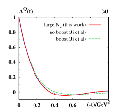
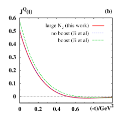
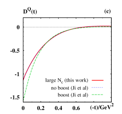
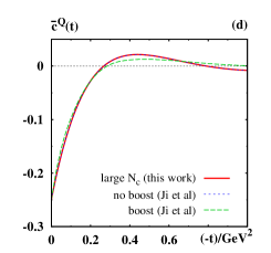
Figure 1: EMT form factors of quarks in the bag model in the large $N_{c}$ limit (solid lines, this work). For comparison we also show results by Ji et al, Ref. Ji:1997gm , computed in the bag model without (dotted lines) and with (dashed lines) considering boosts. This comparison shows the effects of relativistic and $1/N_{c}$–corrections within the “independent particle model treatment” in the bag model. For finite $N_{c}$ there are further corrections associated with the independent particle model treatment, see text.

IV.4 $1/N_{c}$ corrections

The large-$N_{c}$ results are theoretically consistent which is crucial for our study. However, it is instructive to get insights on the size of $1/N_{c}$–corrections by comparing our results with those of Ref. Ji:1997gm obtained for finite $N_{c}$. We can distinguish different types of $1/N_{c}$-corrections. If we do not implement the kinematic effects (18) and large-$N_{c}$ counting rules (19) we recover the “no-boost results” by Ji et al from Ji:1997gm . This type of $1/N_{c}$ correction only affects the form factor $A(t)$ where it has a small effect for $|t|$ below $1\,{\rm GeV}^{2}$, see the curve depicted by the dotted line in comparison to the solid line in Fig. 1a. The form factors $J^{Q}(t)$, $D^{Q}(t)$, $\bar{c}^{Q}(t)$ are not affected by these corrections, so the no-boost results from Ji:1997gm (dotted lines) coincide with our large-$N_{c}$ results (solid lines) in Figs. 1b–d.

A conceptually different type of corrections arises because for finite $N_{c}$ it is necessary to take into account relativistic corrections associated with boosting the quark wave function (14) to a frame where the nucleon moves with velocity $\vec{v}$: $\psi(t,\vec{x})\to S(\Lambda_{\vec{v}})\psi(t^{\prime},\vec{x}{}^{\prime})$ with $S(\Lambda)=\exp(w\gamma^{0}\gamma^{3})$ where $\Lambda_{\vec{v}}$ is the Lorentz transformation for a boost along $z$-axis with $\vec{v}=(0,0,\tanh(w))$ where $\sinh(w)=|\vec{\Delta}|/(2M_{N})$ Ji:1997gm . The results obtained in this way are depicted as dashed lines in Fig. 1. The constraint $J^{Q}(0)=\frac{1}{2}$ is no longer satisfied, see Fig. 1b, because “the boosted bag wave function does not have the correct Lorentz symmetry” Ji:1997gm . This artifact can in principle be avoided using Peierls-Yoccoz projections Peierls:1957er or center-of-mass freedom separation methods Wang:1982tz which were not performed in Ji:1997gm . For our purposes it is completely sufficient to observe that in practice such boost effects — even if they were not entirely consistently estimated in Ji:1997gm — constitute a small correction. It is important to stress that in the large-$N_{c}$ limit $|\vec{\Delta}|/(2M_{N})\to 0$ and this type of relativistic corrections is negligible.

The third type of $1/N_{c}$ corrections is due to the fact that the bag model belongs to a class of so-called independent particle models in which the form factors of one-body operators are strictly speaking zero: the transferred momentum is absorbed by only one “active” quark” while the motion of the remaining “spectator” quarks is not affected. The nucleon wave function of such a configuration is strictly speaking zero. In a more realistic description the nucleon wave-function would contain “correlations” between the constituents through which the momentum transferred to the active quark would be redistributed among all constituents of the system such that the nucleon as a whole would recoil Ji:1997gm . But the bag model quark wave functions are independent of each other, and lack explicit correlations.

At least in principle the bag model could provide correlations: the elastic scattering process could be thought of as consisting of two steps. In the first step the active quark absorbs the transferred momentum. In the second step the active quark “bounces off” the bag boundary, which subsequently transfers momentum to the spectator quarks, etc. Through such back-and-forth bouncing the transferred momentum would be redistributed among all constituents. For larger $|t|$ inelastic processes (bag deformation, creation of $\bar{q}q$-pairs) may become possible. Even though this simple mechanism cannot be expected to be realistic, at least in principle one could estimate correlation effects in this way. In practice this is too complex to consider, and a different way to heuristically estimate correlation effects was chosen in Ji:1997gm : a free parameter $\eta$ was introduced such that the momentum transfer to the active quark is $\vec{\Delta}\to\eta\vec{\Delta}/\cosh(w)$. It is intuitively expected that $\eta\sim 1/3$ to redistribute the momentum transfer among 3 quarks in a recoiled nucleon. A reasonable description of the proton electromagnetic form factors was obtained for $\eta$ in the range of $\eta=$0.35–0.55 with the lower (higher) value yielding a better description of the data at large (intermediate) values of $|t|$ Ji:1997gm . The correlations modeled in this way impact the EMT form factors more strongly than the 2 above-discussed types of $1/N_{c}$ corrections. However, the discrepancy with the general constraints at $t=0$ becomes also more pronounced: e.g. for $\eta=0.35$ one finds $J^{Q}(0)\approx 0.25$ Ji:1997gm instead of $J^{Q}(0)=\frac{1}{2}$ indicating that this method to estimate correlation effects is not trustworthy at small $|t|$, even though it improves the phenomenological description of electromagnetic form factors at $|t|\lesssim 2\,{\rm GeV}^{2}$ Ji:1997gm . As our large-$N_{c}$ results are valid for small $|t|\ll M_{N}^{2}$, while the results for $\eta\neq 1$ from Ji:1997gm are more appropriate at larger $|t|$, a direct comparison is not meaningful and we refrain from it.

Notice that in the large-$N_{c}$ limit also this type of corrections vanish. Let us recall that correlations were introduced to allow the active quark to redistribute the momentum transfer among all constituents such that the entire system changes its direction and the nucleon as a whole is deflected. However, in the leading order of the large-$N_{c}$ limit the momentum transfer is small, $|t|\ll M_{N}^{2}$, and the recoil of the heavy nucleon ($M_{N}\sim N_{c}$) is negligible. Thus, one can consistently evaluate form factors in the bag model without the need to introduce correlations. (Notice that absence of correlations in the large-$N_{c}$ limit is a peculiarity of the bag model. Other models formulated in large-$N_{c}$ limit like the chiral quark soliton or Skyrme models Goeke:2007fp ; Goeke:2007fq ; Wakamatsu:2007uc ; Cebulla:2007ei ; Kim:2012ts ; Jung:2013bya ; Jung:2014jja ; Perevalova:2016dln exhibit strong correlations.)

To summarize, we may regard the results for the EMT form factors shown in Fig. 1 as valid for $|t|\ll M_{N}^{2}$ and theoretically consistent within the bag model in the large-$N_{c}$ limit. These results are subject to $1/N_{c}$ corrections which we may expect to be modest at smaller $|t|$ and more sizable especially at larger $|t|$. Our observations are in line with results from the Skyrme model of Ref. Ji:1991ff where relativistic recoil corrections (to electromagnetic form factors) were also found small for $|t|<1\,{\rm GeV}^{2}$.

V The EMT densities in bag model

In order to compute the EMT densities one can perform the Fourier transforms in Eq. (3). In the large-$N_{c}$ limit in the bag model one can also directly evaluate the EMT matrix elements in coordinate space. Both ways yield the same result for quark EMT densities. But only the direct evaluation in coordinate space allows us to compute the contributions of the “gluons” in ${\cal L}_{G}$ and the “quark-gluon interaction” in ${\cal L}_{\rm surf}$ as defined in (8). We obtain

$$T^{00}_{q}(r) = \frac{N_{q}\,A^{2}}{4\pi}\;\frac{\Omega}{R}\,\biggl{(}\alpha_{+}^{2}j_{0}^{2}+\alpha_{-}^{2}j_{1}^{2}\biggr{)}\,\Theta_{V}\,,$$ (24a)

$$T^{0k}_{q}(\vec{r}) = -\,\frac{1}{2}\;\frac{P_{q}\,A^{2}}{4\pi}\,\biggl{(}2\,\alpha_{+}\alpha_{-}\,\frac{\Omega}{R}\,j_{0}\,j_{1}+\alpha_{-}^{2}\frac{j_{1}^{2}}{r}\biggr{)}\epsilon^{klm}\,e_{r}^{l}\,S^{m}\,\Theta_{V}\,,$$ (24b)

$$T^{ik}_{q}(\vec{r}) = \frac{N_{q}\,A^{2}}{4\pi}\;\alpha_{+}\alpha_{-}\Biggl{(}\biggl{(}j_{0}\,j_{1}^{\prime}-j_{0}^{\prime}\,j_{1}-\frac{j_{0}\,j_{1}}{r}\;\biggr{)}e_{r}^{i}e_{r}^{k}\;+\;\frac{j_{0}\,j_{1}}{r}\;\delta^{ik}\Biggr{)}\,\Theta_{V}\,,$$ (24c)

$$T^{\mu\nu}_{G}(r) = g^{\mu\nu}\;B\;\Theta_{V}\,,$$ (24d)

$$T^{\mu\nu}_{\rm surf}(\vec{r}) = 0\,.\phantom{\Biggl{(}\frac{1}{1}\Biggr{)}}$$ (24e)

For brevity we suppress the arguments of the Bessel functions $j_{i}=j_{i}(\omega\,r/R)$, and primes denote differentiation with respect to $r$. The quark flavor dependence is encoded in the SU(4) spin-flavor factors (17). The contribution of ${\cal L}_{\rm surf}$ vanishes, but we obtain the contribution $T^{\mu\nu}_{G}(r)=g^{\mu\nu}\;B\;\Theta_{V}$ associated with non-fermionic (“gluonic”) effects.

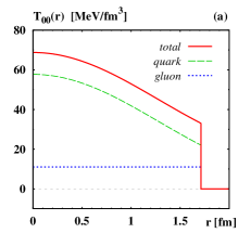
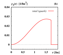
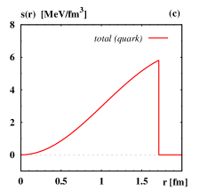
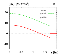
Figure 2: (a) The energy density $T_{00}(r)$, (b) density $\rho_{J}(r)$ characterizing the angular momentum density, (c) shear force distribution $s(r)$, and (d) pressure distribution $p(r)$ as functions of $r$ in the bag model for massless quarks. The vertical lines mark the position of the bag boundary (at $R=1.71\,$fm for massless quarks). In the case of $T_{00}(r)$ and $p(r)$ the contributions from quarks and “gluons” are shown in addition to the total result. For $\rho_{J}(r)$ and $s(r)$ the total result is entirely due to quarks.

V.1 Energy density and mass

The energy density $T_{00}(r)$ receives the contribution $T_{00}^{Q}(r)$ from quarks, Eq. (24a), and a contribution from “gluons” $T_{00}^{G}(r)=B\,\Theta_{V}$ in Eq. (24d). The quark and “gluon” contributions to the energy density are shown in Fig. 2a. The integrated contributions are

$$M_{N}^{Q}=N_{c}\,\varepsilon_{0}\,,\quad M_{N}^{G}=\frac{4\pi}{3}\,R^{3}B\,.$$ (25)

For massless quarks the relative contributions of quarks and “gluons” to the nucleon mass are $M_{N}^{Q}\,:\,M_{N}^{G}=3\,:\,1$. This can be derived in 2 ways: (i) it follows from the nonlinear bag boundary condition (10c). Equivalently, (ii) it can be derived from minimizing the nucleon mass understood as a function of $R$ as follows. Since $\varepsilon_{0}=\omega_{0}/R$ we have

$$M_{N}^{\prime}(R)=\frac{\partial}{\partial R}\biggl{(}N_{c}\,\frac{\omega_{0}}{R}+\frac{4\pi}{3}\,R^{3}B\biggr{)}\stackrel{{\scriptstyle!}}{{=}}0\quad\Leftrightarrow\quad N_{c}\,\omega_{0}=4\pi\,R^{4}B\,.$$ (26)

From Eqs. (25, 26) we see that $M_{N}^{Q}=\frac{3}{4}\,M_{N}$ and $M_{N}^{G}=\frac{1}{4}\,M_{N}$ (for massless quarks). This can be viewed as a bag-model version of the “virial theorem.” We recall that e.g. in soliton models virial theorems are derived by rescaling the coordinates $\vec{r}\to\lambda\vec{r}$ in the functional defining the nucleon mass. Considering infinitisemal variations around $\lambda=1$ leaves the nucleon mass invariant, i.e. $\delta M_{N}=0$. This implies relations among different contributions to the nucleon mass Goeke:2007fp ; Cebulla:2007ei . In the bag model the situation is simpler: the “variation” of the nucleon mass assumes the simple form stated in Eq. (26) for massless quarks. For massive quarks $\omega_{0}=\omega_{0}(mR)$ depends also on $R$ and the virial theorem has a somewhat different form, see App. A.1. Notice that (26) shows that the constant $B={\cal O}(N_{c})$ where one has to keep in mind that the bag radius $R={\cal O}(N_{c}^{0})$ since the size of baryons is of order $N_{c}^{0}$ in the large $N_{c}$ limit.

V.2 Angular momentum density

The components $T_{0k}(\vec{r})$ depend on the nucleon polarization (which we do not indicate for brevity), and receive only a contribution from quarks. The angular momentum density is given by

$$J_{q}^{i}(\vec{r}) = \epsilon^{ijk}r^{j}T^{0k}_{q}(\vec{r})=S^{m}\biggl{[}\delta^{im}\rho^{q}_{J}(r)_{\rm mono}+\,\biggl{(}e_{r}^{i}\,e_{r}^{m}-\frac{1}{3}\delta^{im}\biggr{)}\rho^{q}_{J}(r)_{\rm quad}\biggr{]}\,,$$ (27)

with the monopole Goeke:2007fp and quadrupole Lorce:2017wkb contributions

$$\rho^{q}_{J}(r)_{\rm mono}=-\frac{2}{3}\,\rho^{q}_{J}(r)_{\rm quad}\equiv\rho^{q}_{J}(r),\quad\rho^{q}_{J}(r)=\frac{1}{3}\;\frac{P_{q}\,A^{2}}{4\pi}\;r\,\biggl{(}\frac{2\Omega}{R}\,\alpha_{+}\alpha_{-}j_{0}\,j_{1}+\alpha_{-}^{2}\frac{j_{1}^{2}}{r}\biggr{)}\,\Theta_{V}\,.$$ (28)

The relation $\rho^{q}_{J}(r)_{\rm mono}=-\frac{2}{3}\,\rho^{q}_{J}(r)_{\rm quad}$ is a general result Schweitzer:2019kkd which the bag model respects. The total angular momentum density $\rho_{J}(r)=\sum_{q}\rho^{q}_{J}(r)$ is normalized as $\int\!{\rm d}^{3}r\,\rho_{J}(r)=\frac{1}{2}$ and shown in Fig. 2b.

V.3 Shear forces and pressure

The pressure and shear forces encoded in the stress tensor (5) are given by the expressions

$$p(r) = \Biggl{[}\frac{N_{c}\,A^{2}}{12\pi}\;\alpha_{+}\alpha_{-}\biggl{(}j_{0}j_{1}^{\prime}-j_{0}^{\prime}j_{1}+\frac{2}{r}j_{0}j_{1}\biggr{)}-B\Biggr{]}\,\Theta_{V},$$

$$s(r) = \Biggl{[}\frac{N_{c}\,A^{2}}{4\pi}\;\alpha_{+}\alpha_{-}\biggl{(}j_{0}j_{1}^{\prime}-j_{0}^{\prime}j_{1}-\frac{1}{r}j_{0}j_{1}\biggr{)}\Biggr{]}\,\Theta_{V}.$$ (29)

The numerical results for massless quarks are shown in Figs. 2c and 2d.

In the liquid drop model of a large nucleus which exhibits a “sharp edge” at the radius $R_{\rm nucl}$ the shear force is given by $s(r)=\gamma\,\delta(r-R_{\rm nucl})$ where $\gamma$ is the surface tension Polyakov:2002yz . The nucleon is a far more diffuse object then a large nucleus and Fig. 2c shows that $s(r)$ is consequently much more “spread out” than a $\delta$-function characterizing the shear force distribution of a large nucleus.

In all model calculations so far the pressure was found positive in the inner region and negative in the outer region. This is also the case in the bag model, see Fig. 2d. The positive pressure in the inner region is associated with repulsive forces directed towards outside. The negative pressure in the outer region corresponds to attractive forces directed toward inside. The repulsive and attractive forces must compensate each other according to the von Laue condition which is a necessary condition for stability and will be discussed below in Sec. V.6.

The pressure distribution and the shear forces in Eq. (29) satisfy the differential equation (6). This relation is a consequence of the conservation of the EMT, $\partial_{\mu}T^{\mu\nu}=0$, and hence reflects the fact that in the bag model the EMT is conserved and the description is internally consistent.

V.4 Normal and tangential forces

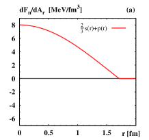
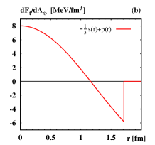
Figure 3: Densities of (a) normal $\!{\rm d}F_{n}/\!{\rm d}A_{r}=\frac{2}{3}s(r)+p(r)$ and (b) tangential $\!{\rm d}F_{t}/\!{\rm d}A_{\vartheta}=\!{\rm d}F_{t}/\!{\rm d}A_{\varphi}=-\frac{1}{3}s(r)+p(r)$ forces per unit area in bag model as functions of $r$. Mechanical stability requires $\frac{2}{3}s(r)+p(r)>0$ inside the bag which is the case.

The stress tensor (5) is a symmetric $3\times 3$ matrix whose eigenvectors are the unit vectors $\vec{e}_{r}$, $\vec{e}_{\vartheta}$, $\vec{e}_{\varphi}$ of the spherical coordinate system and eigenvalues are related to normal and tangential forces Polyakov:2018zvc . For spin-0 and spin-$\frac{1}{2}$ particles the tangential eigenvalues (pertaining to eigenvectors $\vec{e}_{\vartheta}$, $\vec{e}_{\varphi}$) are degenerate with the degeneracy being lifted only for higher spin $J\geq 1$ particles. In our case the normal and tangetial forces per unit area are given by Polyakov:2018zvc

$$T^{ij}\;\!{\rm d}A_{r}^{j} = \frac{\!{\rm d}F_{n}}{\!{\rm d}A_{r}}\;\,\!{\rm d}A_{r}\;e_{r}^{i}=\biggl{(}\frac{2}{3}s(r)+p(r)\biggr{)}\,\!{\rm d}A_{r}\;e_{r}^{i}$$

$$T^{ij}\;\!{\rm d}A_{\vartheta}^{j} = \frac{\!{\rm d}F_{t}}{\!{\rm d}A_{\vartheta}}\;\,\!{\rm d}A_{\vartheta}\;e_{\vartheta}^{i}=\biggl{(}-\frac{1}{3}s(r)+p(r)\biggr{)}\,\!{\rm d}A_{\vartheta}\;e_{\vartheta}^{i}$$ (30)

where $\!{\rm d}\vec{A}_{r}=\!{\rm d}A_{r}\,\vec{e}_{r}$, etc denote the corresponding infinitesimal area elements. The results for normal forces $\!{\rm d}F_{n}/\!{\rm d}A_{r}$ and tangential forces $\!{\rm d}F_{t}/\!{\rm d}A_{\vartheta}=\!{\rm d}F_{t}/\!{\rm d}A_{\varphi}$ are shown in Fig. 3.

Mechanical stability requires that $\!{\rm d}F_{n}/\!{\rm d}A_{r}\geq 0$ with strictly $\!{\rm d}F_{n}/\!{\rm d}A_{r}>0$ at all values of $r$ within the system Perevalova:2016dln . The position where $\!{\rm d}F_{n}/\!{\rm d}A_{r}=0$ marks the “end” of the system Polyakov:2018zvc . In the bag model it is consequently $\!{\rm d}F_{n}/\!{\rm d}A_{r}>0$ for $0\leq r<R$ and the normal force vanishes at the finite radius $r=R$, as shown in Fig. 3a. This is a distinctly different situation than in soliton models where $\!{\rm d}F_{n}/\!{\rm d}A_{r}>0$ for all $0\leq r<\infty$ and the normal forces vanish only in the limit $r\to\infty$ Goeke:2007fp ; Goeke:2007fq ; Wakamatsu:2007uc ; Cebulla:2007ei ; Kim:2012ts ; Jung:2013bya ; Jung:2014jja ; Perevalova:2016dln . Other examples of finite size systems which are analogous in the sense that $\!{\rm d}F_{n}/\!{\rm d}A_{r}$ vanishes at a finite radius are the liquid drop model Polyakov:2002yz and neutron stars whose radius is defined as that value of $r$ where the normal force per unit area (also called the hydrostatic pressure) vanishes Cedric-private .

V.5 Mechanical radius, surface tension, and diffusiveness

The positivity of the normal forces allows one to introduce the notion of a mechanical radius defined as Polyakov:2018zvc

$$\langle r^{2}\rangle_{\rm mech}=\frac{\int\!{\rm d}^{3}r\>r^{2}[\frac{2}{3}s(r)+p(r)]}{\int\!{\rm d}^{3}r\,[\frac{2}{3}s(r)+p(r)]}\,.$$ (31)

We obtain $\langle r^{2}\rangle_{\rm mech}^{1/2}=1.10\,{\rm fm}$ which is smaller than the proton charge radius $\langle r^{2}\rangle_{\rm el}^{1/2}=1.25\,{\rm fm}$ with our parameters. The values of the radii depend on how model parameters are fixed, e.g. a smaller proton charge radius of $1\,{\rm fm}$ was found in Chodos:1974pn with a different parameter fixing. A more robust prediction might be the ratio $\langle r^{2}\rangle_{\rm mech}^{1/2}/\langle r^{2}\rangle_{\rm el}^{1/2}=0.88$ which is independent of how model parameters are fixed (for massless quarks). Interestingly, also the chiral quark soliton model predicts the mechanical radius to be smaller than the proton charge radius (by $25\,\%$ in that model) Polyakov:2018zvc . Notice that the mechanical radius is the same for proton and neutron modulo small isospin violating effects, and hence constitutes a better concept for the nucleon “size” than the charge radius (which is negative for the neutron, giving insights on the distribution of charge inside neutron but not on its size).

One may define the property of “surface tension” for a hadron as

$$\gamma=\int_{0}^{\infty}\!{\rm d}r\,s(r)\,,$$ (32)

if this integral exists. In the bag model we find $\gamma=4.26\,{\rm MeV\,/\,fm^{2}}$. The concept of a surface tension is well-justifed in certain situations, for instance for large nuclei Polyakov:2002yz or $Q$-balls Mai:2012yc . The nucleon is much more diffuse. In order to quantify the “diffusiveness” of a particle we introduce the dimensionless measure $\Delta w^{2}$ for the “skin thickness” of a particle defined in terms of the moments $\langle r^{n}\rangle_{s}$ of the shear force distribution as follows Mai:2012yc

$$\Delta w^{2}=\frac{\bigl{\langle}\,[r^{2}-\langle r^{2}\rangle_{s}]^{2}\bigr{\rangle}_{s}^{1/2}}{\langle r^{2}\rangle_{s}}=\frac{\bigl{[}\langle r^{4}\rangle_{s}-\langle r^{2}\rangle_{s}^{2}\bigr{]}^{1/2}}{\langle r^{2}\rangle_{s}}\,,\quad\langle r^{n}\rangle_{s}=\frac{1}{\gamma}\,\int\!{\rm d}r\,r^{n}s(r)\,.$$ (33)

For a nucleus with a sharp edge in the liquid drop model the shear force is given by $s(r)=\gamma\,\delta(r-R_{A})$ where $R_{A}$ denotes the radius of the nucleus, and $\Delta w^{2}=0$. One also finds $\Delta w^{2}\to 0$ in the limit of very large $Q$-balls Mai:2012yc . For realistic nuclei and finite-size $Q$-balls the “diffusiveness” parameter $\Delta w^{2}$ is small. For the nucleon $\Delta w^{2}=0.48$ in the bag model indicating that the nucleon is much more diffuse than a nucleus, which is not unexpected.

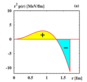
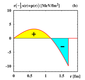
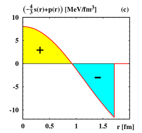
Figure 4: The 3D von Laue condition (a) and its lower-dimensional analogs in 2D (b) and 1D (c) in the bag model for massless quarks. The areas above and below the $r$-axis are equal and compensate each other according to the integrals in Eq. (34).

V.6 EMT conservation: von Laue condition and its lower-dimensional analogs

The pressure and shear forces must obey the following integral relations

$$\int\limits_{0}^{\infty}\!\!{\rm d}r\;r^{2}p(r)=0\;,\quad\int\limits_{0}^{\infty}\!\!{\rm d}r\;r\biggl{(}-\frac{1}{3}\,s(r)+p(r)\biggr{)}=0\;,\quad\int\limits_{0}^{\infty}\!\!{\rm d}r\;\biggl{(}-\frac{4}{3}\,s(r)+p(r)\biggr{)}=0\;.$$ (34)

The first of these relations was introduced by von Laue in Ref. von-Laue and holds in 3D, the other two hold in respectively 2D and 1D and were derived in Polyakov:2018zvc .

The conditions in (34) are proven analytically in App. A.2. The physical interpretation of the first condition in (34) is as follows. The positive pressure in the inner region corresponds to repulsion and the negative pressure in the outer region corresponds to attraction. Mechanical stability requires that the attractive and repulsive forces compensate each other in the 3D integral in (34) which is satisfied in the bag model as shown in Fig. 4a. The tangential force per unit area, $-\frac{1}{3}\,s(r)+p(r)$, must satisfy the 2D relation in (34) which is the case in the bag model as illustrated in Fig. 4b. The interpretation of this condition is that the tangential forces within a 2D slice must compensate each other Polyakov:2018zvc . Similarly also the 1D condition in (34) is satisfied in the bag model, which is illustrated in Fig. 4c. It is also instructive to discuss the “finite-volume von Laue condition” Polyakov:2018zvc

$$\int\limits_{|\vec{r}{}^{\,\prime}|\leq r}\!\!\!\!{\rm d}^{3}r^{\prime}\;p(r^{\prime})=V(r)\,\biggl{(}\frac{2}{3}\,s(r)+p(r)\biggr{)}\,,$$ (35)

where the integration goes over the volume $V(r)=\frac{4}{3}\,\pi\,r^{3}$. The sum rule (35) is satisfied for all $0\leq r<R$. However, in the bag model at $r=R$ one practically deals with the 3D relation in (34). Since $V(R)\neq 0$ is non-zero, this means that the normal force per unit area $\frac{2}{3}\,s(r)+p(r)$ must vanish at the bag boundary, which is the case and emerges here as a necessary condition to comply with the von Laue condition in (34). Notice that $\frac{2}{3}\,s(r)+p(r)$ must vanish at the bag boundary also in order to comply with (6). The differentiation of $\Theta_{V}$-functions in the bag model expressions (29) for $p(r)$, $s(r)$ yields the contribution $\delta(r-R)\,[\frac{2}{3}\,s(r)+p(r)]$ to (6) which must and does vanish at $r=R$.

The integrands $p^{(3D)}(r)=p(r)$, $p^{(2D)}(r)=-\frac{1}{3}s(r)+p(r)$, and $p^{(1D)}(r)=-\frac{4}{3}s(r)+p(r)$ in (34) are special cases of pressures in $n$-dimensional ($nD$) spherically symmetric mechanical systems. In general pressure and shear forces of a $kD$ system are related to those in $nD$ subsystems (if $k<n$ the roles of system and subsystem interchange) as proceeding-new

$$p^{(nD)}(r)=\frac{k}{n}\ p^{(kD)}(r)+\frac{k(n-k)}{n}\;\frac{1}{r^{k}}\int_{0}^{r}dr^{\prime}\ r^{\prime\,k-1}p^{(kD)}(r^{\prime}),$$

$$s^{(nD)}(r)=-\frac{k}{n-1}\ p^{(kD)}(r)+\frac{k^{2}}{n-1}\;\frac{1}{r^{k}}\int_{0}^{r}dr^{\prime}\ r^{\prime\,k-1}p^{(kD)}(r^{\prime}).$$ (36)

The $s^{(nD)}(r)$ and $p^{(nD)}(r)$ in (36) satisfy $\frac{n-1}{n}\frac{\partial\;}{\partial r}s^{(nD)}(r)+\frac{n-1}{r}s^{(nD)}(r)+\frac{\partial\;}{\partial r}p^{(nD)}(r)=0$ and $\int_{0}^{\infty}\!{\rm d}r\;r^{n-1}p^{(nD)}(r)=0$ which are $nD$-versions of respectively (6) and (34). Such relations can be useful e.g. in holographic approaches to QCD or in fractal theories proceeding-new . In the bag model these relations are valid for all $n,\,k>0$ including non-integer and aribtrarily large values. The practical verification of such relations can in practice be numerically challenging especially for large $n$. In the bag model, thanks to the finite range of the densities, it is possible to test the validity and consistency of the relations (36) for any value of $n,\,k>0$ in a non-trivial model.

V.7 EMT conservation: equivalence of $D$-term expressions

The $D$-term can be computed using the expressions in terms of (i) pressure and (ii) shear forces according to Eq. (7). From (29) we find that the two equivalent expressions in Eq. (7) yields the same result which can be written as

$$D=\frac{1}{3}\,M_{N}\,N_{c}\,\frac{A^{2}R^{4}\!}{\omega_{0}^{4}}\;\alpha_{+}\alpha_{-}\biggl{(}-\frac{4}{15}\,\omega_{0}^{3}+\omega_{0}-\frac{2}{5}\,\omega_{0}\,\sin^{2}\omega_{0}-\sin\omega_{0}\,\cos\omega_{0}\biggr{)}\,,$$ (37)

see App. A.3 for a detailed proof. The possibility to compute the $D$-term by means of two different equivalent expressions is also due to EMT conservation. We will discuss the $D$-term in Sec. VI in more detail.

V.8 EMT conservation: form factor $\bar{c}^{G}(t)$

In Sec. IV we found the form factor $\bar{c}^{Q}(t)\neq 0$ from the evaluation of the quark EMT, which means that $T_{\mu\nu}^{Q}$ by itself is not conserved. EMT conservation requires $\sum_{a}\bar{c}^{a}(t)=0$ if one takes into account all contributions in a system, i.e. in the bag model also the contribution of the bag which simulates gluons in the sense discussed in Sec. III. However, while it was straight forward to compute the quark EMT form factors in Sec. IV, it is not clear how to compute the bag contribution to the form factors. At this point we can take advantage of the EMT density framework. Instead of using EMT form factors as an input for an interpretation in terms of EMT densities Polyakov:2002yz , we proceed in the opposite direction and invert Eq. (3) for the “gluon” contribution $T_{\mu\nu}^{G}(r)$ in Eq. (24d). We obtain for massless quarks the result

$$\bar{c}^{G}(t)=\frac{1}{M_{N}}\int\!{\rm d}^{3}r\exp(i\vec{\Delta}\vec{r})\,B\,\Theta_{V}=\frac{3}{4}\;\frac{j_{1}(qR)}{qR}\;,\quad q=\sqrt{-t}$$ (38)

where we eliminated the bag constant $B$ by means of Eq. (26). From the behavior of spherical Bessel functions for small arguments $j_{l}(z)=z^{l}/(2l+1)!!+{\cal O}(z^{l+2})$ we find $\bar{c}^{G}(0)=\frac{1}{4}$ to be compared with $\bar{c}^{Q}(0)=-\,\frac{1}{4}$, see Sec. IV.3 and Fig. 1d. In App. A we show that we have $\forall\;t$

$$\bar{c}^{Q}(t)+\bar{c}^{G}(t)=0\,$$ (39)

as it is required by the conservation of the total EMT.

VI The $D$-term

In this Section we discuss the $D$-term for the nucleon and other hadrons, and we consider then several instructive limiting cases in the bag model. Here and throughout in Secs. VI.1–VI.6 we consider massless quarks. In Sec. VII we will discuss also $m\neq 0$. The expression for the $D$-term of the nucleon was already quoted in (37). Let us generalize this result to a general state. Mesons (baryons) are constructed in the bag model by placing a $\bar{q}q$ ($qqq$) in the bag in a color singlet state. The mass and bag radius of a general bag model state (for massless quarks) are given by

$$M=\frac{4}{3}\,\frac{\sum_{i}\omega_{i}}{R}\,,\quad R=\biggl{(}\frac{\sum_{i}\omega_{i}}{4\pi B}\biggr{)}^{1/4}$$ (40)

which follows from the virial theorem (26). For baryons the summation goes over $N_{c}=3$ occupied bag levels $\omega_{i}$, for mesons over two levels. The bag constant is fixed as $B=0.0559\,{\rm fm}^{-4}$ to reproduce the nucleon mass. Inserting the expressions for the normalization constant $A$ and $\alpha_{\pm}$ defined in (11) and mass (40) into Eq. (37) we obtain the result for the $D$-term of a general bag model state (made of massless quarks)

$$D=-\,\frac{4}{5}\times\biggl{[}\sum\limits_{i=1}^{N_{\rm cons}}\omega_{i}\biggr{]}\;\biggl{[}\sum\limits_{i=1}^{N_{\rm cons}}\frac{\omega_{i}(4\,\omega_{i}^{2}-15)+6\,\omega_{i}\,\sin^{2}\omega_{i}+15\,\sin\omega_{i}\,\cos\omega_{i}}{54\,\omega_{i}(\omega_{i}-1)\sin^{2}\omega_{i}}\biggr{]}\,.$$ (41)

We make two important observations. First, since $\omega_{i}\geq\omega_{0}\approx 2.04$ it is $D<0$ for all hadron states constructed in the bag model including unstable resonances. This is in line with results from all theoretical studies so far. Second, the dependence on the model parameter bag radius $R$ or bag constant $B$ cancels out in the $D$-term which therefore only depends on the dimensionless numbers $\omega_{i}$ (for massless quarks, cf. Sec. VII for the case of massive quarks).

VI.1 The $D$-term of the nucleon

For the nucleon we obtain from (37, 41) in the case of massless quarks the result

$$D_{\rm nucleon}=-1.145\,,$$ (42)

which is in agreement with the numerical bag model calculation of nucleon GPDs and EMT form factors in Ref. Ji:1997gm . The magnitude of the nucleon $D$-term in the bag model is smaller compared to soliton models Goeke:2007fp ; Goeke:2007fq ; Wakamatsu:2007uc ; Cebulla:2007ei ; Kim:2012ts ; Jung:2013bya ; Jung:2014jja ; Perevalova:2016dln . This is not surprizing considering that $D=M_{N}\int\!{\rm d}^{3}r\;r^{2}p(r)$ is sensitive to long distances. In fact, in chiral models $|D|$ is larger in the chiral limit where $p(r)$ and $s(r)\propto$ $1/r^{6}$. For finite pion masses $m_{\pi}$ the densities decay exponentially like $e^{-m_{\pi}r}$. The range of internal forces decreases in the soliton models, and $|D|$ diminishes Goeke:2007fp . Since the bag model has a finite radius, the value for $|D|$ is small. We remark that through the SU(4) spin-flavor factors (17) the bag model complies with the large-$N_{c}$ predictions Goeke:2001tz

$$(D^{u}+D^{d})_{\rm nucleon}={\cal O}(N_{c}^{2}),\quad(D^{u}-D^{d})_{\rm nucleon}={\cal O}(N_{c}).$$ (43)

VI.2 $\rho$ meson

Placing in the lowest level of the bag a $\bar{q}q$ pair with aligned spins yields a state with the quantum numbers of a $\rho$-meson. With $B$ fixed to reproduce the nucleon mass yields a mass of 692 MeV which agrees with the experimental value of the $\rho$-meson mass 775 MeV within 10$\,\%$. Other ways to fix model parameters can also be considered Hasenfratz:1977dt . In contrast to this there is no ambiguity as to the bag model prediction for the $D$-term (41) which does not depend on the bag radius $R$ or bag constant $B$. The model prediction is

$$D_{\rho\mbox{-}\rm meson}=\frac{4}{N_{c}^{2}}\,D_{\rm nucleon}=-0.509\,.$$ (44)

Recalling that $D_{\rm nucleon}={\cal O}(N_{c}^{2})$, cf. (43), we see that the $D$-term of the $\rho$-meson (and all mesons) is of ${\cal O}(N_{c}^{0})$.

As there is no spin-spin interaction a $\bar{q}q$ pair with anti-aligned spins corresponding to a state with pion quantum numbers has exactly the same mass (and $D$-term) as the $\rho$-meson. However, since the bag boundary does not respect chiral symmetry, the description of the pion in the bag model is inadequate. This becomes evident here in two ways. First, in the chiral limit the pion is massless while here it remains massive and is mass-degenerate with the $\rho$-meson. Second, soft pion theorems predict $D_{\rm pion}=-1$ Novikov:1980fa ; Voloshin:1980zf ; Voloshin:1982eb ; Leutwyler:1989tn while in the bag model one would obtain the same value as in (44). Ways to construct light pion states have been discussed Donoghue:1979ax . The cloudy bag model Thomas:1982kv reconciles the bag concept and chiral symmetry. Both approaches are beyond the scope of this work. In any case, since it is not a Goldstone boson one may apply the bag model to the description of the $\rho$-meson with less reservations. It will be interesting to test the bag model prediction $D_{\rho\mbox{-}\rm meson}\,:\,D_{\rm nucleon}=4\,:\,9$ in other models or lattice QCD.

Notice that a spin-1 hadron like the $\rho$-meson has 6 form factors of the total EMT Abidin:2008ku ; Polyakov:2019lbq ; Cosyn:2019aio . Our $D_{\rho\mbox{-}\rm meson}$ corresponds to the form factors $D_{0}(t)=-\,{\cal G}_{3}(t)$ in the notations of respectively Polyakov:2019lbq or Cosyn:2019aio . Studies of other $\rho$-meson EMT form factors will be left to future investigations.

VI.3 $\Delta$-resonance

Let us briefly also comment on the $D$-term of the $\Delta$-resonance. As discussed in the previous section, due to absence of spin-spin interactions states differing by the spin quantum numbers are degenerate. In particular, also the $\Delta$-resonance and the nucleon are degenerate, and the $D$-term of the $\Delta$ is simply predicted to be

$$D_{\Delta\mbox{-}\rm resonance}=D_{\rm nucleon}=-1.145\,.$$ (45)

Even though the absolute value might be underestimated, the bag model result $D_{\Delta\mbox{-}\rm resonance}=D_{\rm nucleon}$ is correct in large-$N_{c}$ Perevalova:2016dln . This is another consistency test of the large-$N_{c}$ description of baryons in the bag model.

VI.4 Roper resonance

The state $N(1440)$ known as Roper resonance has the quantum numbers of the proton $J^{P}=\frac{1}{2}{}^{+}$ but a 50$\,\%$ larger mass and its structure “has defied understanding” since its discovery in the 1960s, see the review Burkert:2019bhp . In the bag model it is described by placing two quarks in the ground state with $\omega_{0}=2.04$ and one quark in the first excited state with $\omega_{1}=5.40$. If one would use the same bag radius for the nucleon and the Roper, then the physical value of the Roper mass would be reproduced. A more consistent parameter treatment may be to use the same bag constant $B$ for nucleon and Roper, which yields a Roper mass of 1302 MeV and underestimates the physical value by 10$\,\%$. This is not unreasonable for such a simple model. While the mass increases by about 50$\,\%$, the pressure in the center increases by a factor of 7.5 as one goes from the ground state nucleon to the first excited state in the $J^{P}=\frac{1}{2}{}^{+}$ sector. The increase of the internal forces is reflected by an increase of the $D$-term for which Eq. (41) yields the value

$$D_{\rm Roper}=5.846\,D_{\rm nucleon}=-6.695\,.$$ (46)

It is interesting to observe how strongly the $D$-term is varied as one goes from a ground state to an excited state within a theory. This is mainly due to an increase of internal forces, and in line with studies of excited states in $Q$-ball systems Mai:2012cx . It is not known how the $D$-term of the Roper can be studied in experiment, but it would be interesting to confront the prediction (46) with results from other models or lattice QCD. We remark that $\Delta w^{2}$ defined in (33) is for Roper $\Delta w^{2}=0.72$ showing that this state is even more diffuse than the nucleon, as intuitively expected.

VI.5 Negative parity baryons

The lightest baryon with quantum numbers $J^{P}=\frac{1}{2}{}^{-}$ is $N(1535)$. Negative parity solutions to the bag equations (10) are given by the same expression as positive parity solutions (11), but with upper and lower components exchanged and with the $\omega_{i}$ obtained from (for massless quarks) the transcendental equation $\omega=(1+\omega)\,\tan\omega$ whose lowest energy solution is $\omega=3.81$. Keeping $B$ fixed at the value required for the nucleon yields 1498 MeV and reproduces the mass of $N(1535)$ within $3\,\%$. Also here is the $D$-term independent of parameter fixing and we obtain

$$D_{N(1535)}=11.32\,D_{\rm nucleon}=-12.97$$ (47)

which confirms the trend that the $D$-terms grow for heavier excited states in the spectrum of a theory. Also in this case we are not aware of a practical method to learn about the $D$-term of the state $N(1535)$ from experiment. However, the interesting prediction $D_{N(1535)}=11.32\,D_{\rm nucleon}$ could be compared to theoretical studies in other models. With $\Delta w^{2}=0.59$ this state is somewhat less diffuse than the Roper.

VI.6 Highly excited states in baryonic spectrum

In this section we consider higher excited states in the bag model. While we do not expect a realistic description of the hadronic spectrum, the bag model provides a consistent theoretical framework and it is instructive to explore it. For simplicity we consider massless quarks and limit ourselves to the positive parity baryons sector.

As mentioned in the context of Eq. (41), we find $D<0$ for all excited states. Another important observation is that the $D$-terms grow quickly with the mass of the hadron. To illustrate this point we plot the $D$-terms vs masses for $J^{P}=\frac{1}{2}{}^{+}$ baryons made of massless $u$- and $d$-quarks in Fig. 5 which shows the first 4000 states: the first state is the nucleon with $(M,\;D)=(938\,{\rm MeV},\;-1.145)$ and last state has $(M,\;D)=(10.9\,{\rm GeV},\;-3068)$. All states above $2\,{\rm GeV}$ are hypothetical and practically in the continuum. Each state has a twofold degeneracy due to isospin quantum numbers. (In our large-$N_{c}$ treatment the spectrum of $J^{P}=\frac{3}{2}{}^{+}$ baryons looks exactly the same with a four-fold degeneracy due to isospin $\frac{3}{2}$ of $\Delta$-states.) While the baryon masses increase by one order of magnitude in the range considered in Fig. 5, the $D$-terms grow by 4 orders of magnitude. This is in line with results from $Q$-balls Mai:2012cx .

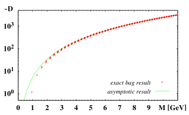
Figure 5: $(-D)$ vs mass for the first 4000 states in the positive parity sector for states made of massless up- and down-quarks. While the masses increase by one order of magnitude, the $D$-terms grow by 4 orders of magnitude. The analytically derived asymptotic result (50) for the $D$-term is shown as solid line. The degeneracy pattern of the states is explained in the text.

To get more insight we discuss the EMT densities of a (hypothetical) highly excited nucleon state. For $Q$-balls it was observed that $T_{00}(r)$ of the $N^{\rm th}$ (radial) excitation exhibits characteristic structures with $N$-shells surrounding a “core” region, while $p(r)$ exhibits $(2N+1)$-nodes where $N=0$ refers to the ground state Mai:2012cx . Is this also the case for excited states in the bag? The answer is no. For illustration we show in Fig. 6 the EMT densities for the state with the level $\omega_{15}$ tripply occupied. This corresponds to a hypothetical $3163^{\rm th}$ excited state above the nucleon (ground) state with $(M,\,D)=(10.2\,{\rm GeV},\,-2608)$. The EMT densities exhibit characteristic “wiggles” but $p(r)$ exhibits only one node. This is a general result: no matter how highly excited a bag state is, $p(r)$ crosses zero only once. Clearly, the spectrum of excitations in the bag model has a much different structure than the $Q$-ball system Mai:2012cx . One expects such highly excited states to be very diffuse and the result $\Delta w^{2}=2.9$ for this hypothetical state confirms it.

The solutions to the transcendental equation (12) are approximated by $\omega_{j}\to(j+3/4)\,\pi$ for massless quarks to within an accuracy of better than $2\,\%$ already for $j\geq 1$. For $\omega_{15}$ this asymptotic formula has an accuracy of $2\times 10^{-4}$. Evaluating the expressions for $T_{00}(r)$, $p(r)$, $s(r)$ in Eqs. (24a, 24d, 29) for asymptotically large $\omega_{j}$ yields

$$\biggl{[}r^{2}T_{00}(r)\biggr{]}_{\rm asymp} = \frac{\sum_{j}\omega_{j}}{4\pi R^{2}}\;\biggl{(}1+\frac{r^{2}}{R^{2}}\biggr{)}\,\Theta_{V}\,,$$

$$\biggl{[}\,r^{2}p(r)\,\biggr{]}_{\rm asymp} = \frac{\sum_{j}\omega_{j}}{4\pi R^{2}}\;\biggl{(}\frac{1}{3}-\frac{r^{2}}{R^{2}}\biggr{)}\,\Theta_{V}\,,$$

$$\biggl{[}r^{2}s(r)\biggr{]}_{\rm asymp} = \frac{\sum_{j}\omega_{j}}{4\pi R^{2}}\;\Theta_{V}\quad\mbox{for}\quad\omega_{j}\to(j+3/4)\,\pi$$ (48)

where $R$ is defined in Eq. (40) and it is understood that all quantities actually depend on a set of 3 (or 2) values of $\omega_{j}$ for a higher baryonic (or mesonic) excitation. Except for the small-$r$ region the asymptotic expressions yield a good description of the gross features of the exact densities as shown in Fig. 6.

Remarkably, the asymptotic expression for $T_{00}(r)$ integrates to the exact expression for the baryon mass in Eq. (40). The asymptotic expressions for pressure and shear forces satisfy the differential equation (6), and $p(r)_{\rm asymp}$ complies with the von Laue condition albeit not with its lower-dimensional analogs in (34) where the exact small-$r$ details are essential. The asymptotic normal force $r^{2}[\frac{2}{3}\,s(r)+p(r)]_{\rm asymp}=(\sum_{j}\omega_{j})(1-r^{2}/R^{2})/(4\pi R^{2})\,\Theta_{V}>0$ for $r<R$ and vanishes at $r=R$. The two equivalent expressions in Eq. (7) yield the same asymptotic result for the $D$-term

$$D_{\rm asymp}=-\frac{16}{135}\,\biggl{(}\sum_{j}\omega_{j}\biggr{)}^{2}\;.$$ (49)

The energy mean square radius and mechanical radius are $\langle r_{E}^{2}\rangle_{\rm asymp}=\frac{2}{5}\,R^{2}$ and $\langle r_{\rm mech}^{2}\rangle_{\rm asymp}=\frac{1}{5}\,R^{2}$. Finally, by exploring Eq. (40), we may eliminate the sum $\sum_{j}\omega_{j}$ in (49) in favor of $M$ which yields (for mesons and baryons)

$$D_{\rm asymp}=-\,A\,M^{\,8/3}$$ (50)

with $A=\frac{1}{5}(16\pi\sqrt{3}\,B)^{-2/3}$. This asymptotic expression explains the strong rise of $D$ with the mass observed in Fig. 5 where Eq. (50) is depicted as solid line. Interestingly the spectrum of radial $Q$-ball excitations exhibits the same asymptotic relation: for the $N^{\rm th}$ excitation the $Q$-ball mass grows like $M\propto N^{3}$ and $D$-term as $D\propto-\,N^{8}$, such that $D\propto-\,M^{8/3}$ Mai:2012cx like in bag model. But the internal structure of the excitations is much different: e.g. the $p(r)$ of the $N^{\rm th}$ excited $Q$-ball state exhibits $(2N+1)$ Mai:2012cx , while the $p(r)$ of excited bag states have always only one node.

To end this section we comment on the near-degeneracies visible in Fig. 5 where the first 4000 states in the $J^{P}=\frac{1}{2}{}^{+}$ sector appear to be organized in a far smaller set of near-degenerate multiplets. To understand these near-degeneracies we notice that $\omega_{j}\approx(j+3/4)\,\pi$ for $j\gtrsim 1$ can be further simplified as $\omega_{j}\approx j\,\pi$ for large enough $j\gg 1$. If always all three occupied levels $j_{1}$, $j_{2}$, $j_{3}$ complied with this condition then the mass would be determined by three integers as $M\approx{\rm const}\,(j_{1}+j_{2}+j_{3})^{3/4}$ and the $n^{\rm th}$ energy level would be $\frac{1}{2}n(n+1)(n+2)$–fold degenerated (like 3D harmonic oscillator formulated in Cartesian coordinates). Since for lower bag levels $j\gg 1$ is of course not valid, in practice a lesser degeneracy pattern is realized in Fig. 5.

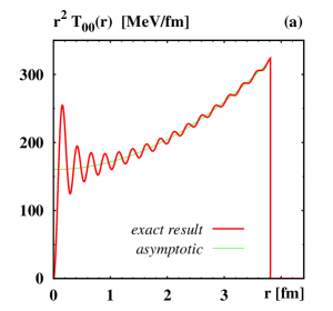
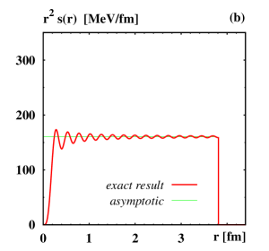
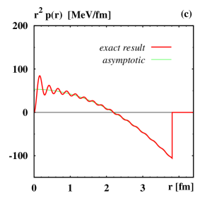
Figure 6: Solid lines: EMT densities $r^{2}T_{00}(r)$, $r^{2}s(r)$, $r^{2}p(r)$ for a (hypothetical) highly excited nucleon state with the tripply occupied bag level $\omega_{15}=49.47\approx(j+3/4)\,\pi$ with $j=15$. For this state the bag radius is $R=3.8\,{\rm fm}$, mass $M=10.24\,{\rm GeV}$, $D$-term $D=-2607.7$ to be compared with the nucleon ground state where $\omega_{0}=2.04$, $R=1.71\,{\rm fm}$, $M=938\,{\rm MeV}$, $D=-1.145$. Thin lines: asymptotic results for the bag model densities from Eq. (48) for $\sum\omega_{j}=3\omega_{15}$ and $R$ as given by Eq. (40).

VII Limiting cases

In this section we assume that $mR\neq 0$. The lowest solution $\omega_{0}$ of the transcendental equation (12) depends on the product $mR$. We will be especially interested in the limit $\varepsilon=1/(mR)\to 0$ where we have $\omega_{0}\to\pi$. For our calculation the $\varepsilon$-corrections to $\omega_{0}$ are essential. They can be determined analytically, and are given by

$$\omega_{0}=\pi-\frac{\pi}{2}\,\varepsilon+\frac{\pi^{3}}{6}\,\varepsilon^{3}-\frac{7\pi^{4}}{48}\,\varepsilon^{4}+\frac{\pi^{3}}{2}\biggl{(}\frac{1}{16}-\frac{\pi^{2}}{5}\biggr{)}\,\varepsilon^{5}+\frac{109\,\pi^{5}}{480}\,\,\varepsilon^{6}+{\cal O}(\varepsilon^{7}),\quad\mbox{for}\quad\varepsilon=\frac{1}{mR}\ll 1.$$ (51)

After exploring the virial theorem for $m\neq 0$ in Eq. (62) of App. A the bag constant becomes

$$B=\frac{N_{c}}{4R^{3}}\;\kappa\,\biggl{(}\varepsilon+{\cal O}(\varepsilon^{2})\biggr{)},\quad\kappa=\frac{\pi}{R},\quad c_{0}=\frac{\pi}{2R^{3}}\,$$ (52)

where we also define a constant $c_{0}$ which will be used in the subsequent equations. For the EMT densities we obtain in the region $0\leq r\leq R$ for $\varepsilon\ll 1$ the results

$$T_{00}(r) = N_{c}\,m\;c_{0}\,j_{0}(\kappa r)^{2}+\dots\;,$$

$$\rho_{J}(r) = \frac{1}{3}\;c_{0}\;\kappa r\;j_{0}(\kappa r)j_{1}(\kappa r)+\dots\;,$$

$$s(r) = \frac{N_{c}\kappa}{2m}\;c_{0}\biggl{(}-j_{0}^{\prime}(\kappa r)j_{1}(\kappa r)-\frac{1}{r}\,j_{0}(\kappa r)j_{1}(\kappa r)+j_{0}(\kappa r)j_{1}^{\prime}(\kappa r)\biggr{)}+\dots\;,$$

$$p(r) = \frac{N_{c}\kappa}{6m}\;c_{0}\biggl{(}-j_{0}^{\prime}(\kappa r)j_{1}(\kappa r)+\frac{2}{r}\,j_{0}(\kappa r)j_{1}(\kappa r)+j_{0}(\kappa r)j_{1}^{\prime}(\kappa r)\biggr{)}-\frac{N_{c}\kappa}{4mR^{4}}\;,+\dots$$ (53)

where the dots indicate subleading terms. For $r>R$ the densities are zero due to the $\Theta_{V}$ not shown here for brevity. Notice that $T_{00}(r)={\cal O}(\varepsilon^{-1})$ and the dots indicate terms of ${\cal O}(\varepsilon^{0})$, $\rho_{J}(r)={\cal O}(\varepsilon^{0})$ and the dots indicate terms of ${\cal O}(\varepsilon)$, while $p(r)$ and $s(r)$ are both of ${\cal O}(\varepsilon)$ with dots indicating terms of ${\cal O}(\varepsilon^{2})$.

Integrating $T_{00}(r)$ in (53) over the volume yields

$$M_{N}=\frac{N_{c}}{R}\biggl{(}\varepsilon^{-1}+\frac{5}{6}\,\pi^{2}\varepsilon+{\cal O}(\varepsilon^{2})\biggr{)}=N_{c}\,m\biggl{(}1+\frac{5}{6}\,\pi^{2}\varepsilon^{2}+\dots\biggr{)}\,.$$ (54)

The term of ${\cal O}(\varepsilon^{0})$ contributing to $T_{00}(r)$ in (53) integrates exactly to zero, and the limit $M_{N}=N_{c}m$ is approached from above, i.e. with positive ${\cal O}(\varepsilon)$ corrections. Integrating $\rho_{J}(r)$ in (53) over the volume yields the nucleon spin $\int\!{\rm d}^{3}\rho_{J}(r)=\frac{1}{2}$ up to the order at which the expansion (51) of $\omega_{0}$ is truncated (if one does not expand the exact expression for $\rho_{J}(r)$ integrates of course to $\frac{1}{2}$ “to all orders”). The pressure and shear forces in (53) comply with the von Laue condition and the lower dimensional conditions in (34) also up to the order at which the expansion of $\omega_{0}$ in (51) is truncated (and are of course also valid to all orders if we do not expand).

Notice that the virial theorem is always valid as long as $\varepsilon\neq 0$. In the expansions in (53) the connection to the virial theorem is not visible. The leading term in $M_{N}=N_{c}m+\dots$ is irrelevant for the virial theorem and drops out from $M_{N}^{\prime}(R)$. Stability, pressure and the von Laue condition are all encoded in the subsubleading terms of ${\cal O}(\varepsilon)$ in $T_{00}(r)$ in (53). This explains why the energy density is of ${\cal O}(\varepsilon^{-1})$ but the pressure and shear forces are of ${\cal O}(\varepsilon)$.

Using the expansion for $p(r)$ and $s(r)$ in (53) we obtain from (7) the result

$$D=-\;N_{c}^{2}\,\biggl{(}\frac{4\,\pi^{2}-15}{45}-\frac{2\pi^{2}}{15}\,\varepsilon+{\cal O}(\varepsilon^{2})\biggr{)}\,.$$ (55)

The limit of the $D$-term in Eq. (55) applies to three different situations:

(i) $$\mbox{$\;R=\mbox{fixed}$, \ \ $m\to\infty$},$$

(ii) $$\mbox{$\,m=\mbox{fixed}$, \ \ $R\to\infty$},$$

(iii) $$\mbox{$m\to\frac{1}{3}\,M_{N}$, $\,R\to\infty$, \ $M_{N}=\mbox{fixed}$},$$ (56)

to be discussed below. The limits (i) and (ii) were briefly discussed in Hudson:2017oul . The Figs. 7a–c show how $m$, $R$, $M_{N}$ are correlated in those limits. The Figs. 7d–f show the behavior of the $D$-term.

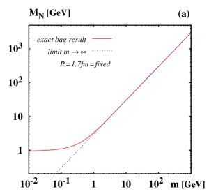
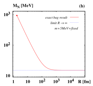
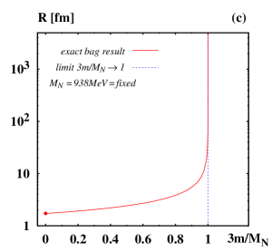
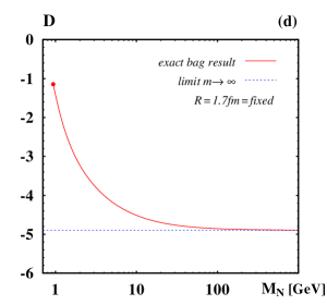
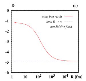
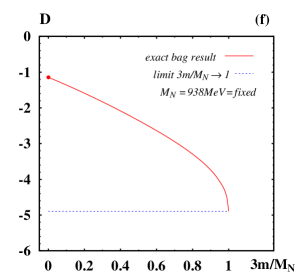
Figure 7: (a) $M_{N}$ as function of quark mass $m$ for fixed $R=1.7\,{\rm fm}$. (b) $M_{N}$ as function of bag radius $R$ for fixed $m=5\,{\rm MeV}$. (c) $R$ vs. $m$ (in units of $\frac{1}{3}M_{N}$) for fixed $M_{N}=938\,{\rm MeV}$. (d) The $D$-term vs $M_{N}$ for fixed $R=1.7\,{\rm fm}$. (e) The $D$-term vs $R$ for a fixed $m=5\,{\rm MeV}$. (f) The $D$-term vs $m$ (in units of $\frac{1}{3}M_{N}$) for fixed $M_{N}=938\,{\rm MeV}$. The “physical point” with $M_{N}=938\,{\rm MeV}$, $R=1.7\,{\rm fm}$ is marked (this point corresponds to $m=5\,{\rm MeV}$ in (b), (d) and zero else).

The case (i) in (56) corresponds to the “heavy quark limit” where the nucleon mass $M_{N}\to N_{c}\,m$ becomes large, see Fig. 7a. For $m\gtrsim 1\,{\rm GeV}$ we have $M_{N}\approx N_{c}\,m$ with a $10\,\%$ or better accuracy. The asymptotics $M_{N}=N_{c}\,m$ is shown as dashed line in Fig. 7a. This is intuitively expected: in the heavy quark limit one expects that hadron masses are largely due to the heavy quark mass. In this limit the quarks become “non-relativistic:” it is $\alpha_{+}={\cal O}(\varepsilon^{0})$ while $\alpha_{-}={\cal O}(\varepsilon)$ such that the upper component of the spinor (11) dominates and the lower component goes to zero. Interestingly, the $D$-term is proportional to $\alpha_{+}\alpha_{-}$, see Eq. (37), but does not vanish because $M_{N}\propto\varepsilon^{-1}$ also enters its definition, see Eq. (7). Thus $D\propto M_{N}\alpha_{+}\alpha_{-}$ has a non-zero limit, see (55). In Fig. 7d we show how the $D$-term changes as one varies the quark mass from $m=0$ up to $1\,{\rm TeV}$, with the asymptotic result (55) shown as dashed line.

In the limit (ii) in (56) the boundary is moved to infinity for fixed $m$ chosen to be $5\,{\rm MeV}$ in Fig. 7b. Intuitively one would expect to recover “free quarks” as the boundary is moved further and further away and the system becomes more and more loosely bound. Indeed, also here $M_{N}\to N_{c}\,m$ (though in contrast to limit (i) the quarks may still be relativistic since $m$ does not need to be large as long as it is non-zero). This limit is approached from above according to Eq. (54) as shown in Fig. 7b where $R$ is varied from $1.7\,{\rm fm}$ up to $1\,$Å with the asymptotic result $M_{N}=N_{c}\,m$ shown as dashed line. Also in this limit the $D$-term approaches the asymptotic value (55) as shown in Fig. 7e. Remarkably, the $D$-term of a free fermion is zero Hudson:2017oul , but here we do not recover this result, even though we deal with a more and more loosely bound system. The reason is as follows. As $R$ becomes large the “confinement” of the fermions inside an increasingly large cavity becomes less and less important, and the mass of the bound state approaches $M_{N}\to N_{c}\,m$. But no matter how small the “residual interactions” in an increasingly large cavity are: they remain non-zero, enter the description of the internal shear and pressure forces, and generate a non-zero $D$-term. How this happens can be traced back on the technical level through, for instance, the virial theorem, see Appendix A. To recover a free theory one has to take the limit $R\to\infty$ much earlier, on the Lagrangian level in Eq. (8) Hudson:2017oul .

The limit (iii) in (56) is also very interesting. Here we assume throughout a system with the fixed (physical) value of the nucleon mass, but we allow the model parameters $m$, $R$ to vary such that the internal model dynamics interpolates all the way from highly relativistic ($m=0$) to highly non-relativistic ($m\to\frac{1}{3}M_{N}$). In the bag model the physical situation is of course more realistically reproduced for highly relativistic quarks rather than for non-relativistic ones. But it is insightful to investigate such a transition from highly to non-relativistic system within a quark model. A convenient measure for this transition is $m$ expressed in units of $\frac{1}{3}\,M_{N}$, i.e. the variable $3m/M_{N}$ whose range is $0\leq 3m/M_{N}\leq 1$. When $3m/M_{N}\to 0$ we deal with highly relativistic (massless) quarks in a relatively small system of radius $R=1.7\,{\rm fm}$ which corresponds to the “physical situation” in this model. When $3m/M_{N}\to 1$ we deal with a trully non-relativistic model of the nucleon: in this limit the nucleon mass is $100\,\%$ due to the “constituent quark mass.” In order to maintain in this limit the fixed (physical) value of the nucleon mass (in a system where the mass of the bound state is nearly entirely due to the mass of its constituents), it is necessary that the system becomes more loosely bound which implies that the size of the system must increase. In the strict limit $m\to\frac{1}{3}\,M_{N}$ the bag radius diverges. The connection of $m$ (in units of $\frac{1}{3}\,M_{N}$) and $R$ for fixed $M_{N}=938\,{\rm MeV}$ is shown in Fig. 7c. For instance, if we wanted $99.999\,\%$ of nucleon mass to be due to the constituent quark masses, then $R=0.57\,\mu{\rm m}$ would be required. It should be stressed that, while the system becomes more loosely bound in the sense that the binding energy decreases, we nevertheless still have confinement (in the specific way it is modelled in the bag model; it should be kept in mind that the binding energy is positive in a confining system). Since in the limit (iii) it is $m\to\frac{1}{3}\,M_{N}$ while $R\to\infty$ the $D$-term is again given by the limit $mR\to\infty$ quoted in Eq. (55). How the $D$-term behaves during the transition from a highly relativistic ($3m/M_{N}=0$) to a highly non-relativistic ($3m/M_{N}\to 1$) system with fixed $M_{N}$ is shown in Fig. 7f. For the last point included in this figure it is $M_{N}-3m=10\,\rm eV$ and $R=4\,\mbox{\AA}$, which are numbers natural for systems in atomic physics.

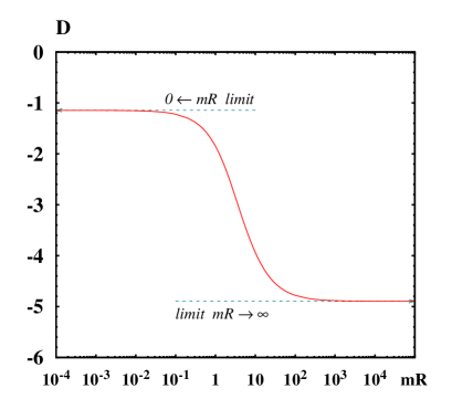
Figure 8: The $D$-term vs $mR$ in the bag model. As a dimensionless quantity the $D$-term only depends on the bag model parameters $m$ and $R$ through the dimensionless variable $mR$.

The way the limiting value (55) of the $D$-term is approached in Figs. 7d–f is characteristic for the three different limits in (56). When we plot $D$ as function $mR$, the results from Figs. 7d–f are in all 3 cases on a single universal curve shown in Fig. 8. Since $D$ is dimensionless. it can only depend on the bag model parameters $m$ and $R$ in terms of the dimensionless variable $mR$. It is shown in Fig. 8 how the $D$-term depends on this dimensionless variable $mR$. The “physical situation” for the proton corresponds to the limit $mR\to 0$ (fixed $R=1.7\,{\rm fm}$ and light or massless up- and down-quarks). The limit $mR\to\infty$ can refer to the 3 different limiting cases in (56) discussed above.

One limiting case remains to be mentioned: fixed $m$ and $R\to 0$. In this limit one obtains a “point-like” particle whose mass diverges as $M_{N}\propto\frac{1}{R}$. This divergence is analogous to the difficulties associated with the description of point-like particles or point-like electric charges in classical physics. The description of the “internal structure” in a “point-like particle” is of no immediate interest. We therefore refrain from discussing this limit further. The result for the $D$-term in this peculiar limit is, however, also shown in Fig. 8 in the direction $mR\to 0$.

VIII Counter-example Bogoliubov model

In all theoretical approaches so far the $D$-terms of particles were found negative, except for free fermion fields where $D=0$ Hudson:2017oul . It is an interesting question whether positive $D$-terms can be realized at all in a physical system.

In fact, positive $D$-terms were found for unphysical states with spin and isospin $S=I\geq\frac{5}{2}$ in the rigid rotator approach in the Skyrme model Perevalova:2016dln . Hadronic states with such (“exotic”) quantum numbers are artifacts of the rigid rotator approach and not realized in nature. When computing masses and other properties of such states one notices nothing unusual. But a more careful investigation of the EMT densities reveals why these states are unphysical: they do not obey the basic mechanical stability criterion, namely the positivity of normal forces $\frac{2}{3}\,s(r)+p(r)>0$. So the rigid rotator states with $S=I\geq\frac{5}{2}$ have positive $D$-terms, but they are also unphysical Perevalova:2016dln .

Despite its simplicity and drawbacks the bag model is from the point of view of mechanical stability a perfectly reasonable and theoretically consistent framework with negative $D$-term. However, a model which in some sense may be viewed as a predecessor of the bag model Thomas:2001kw , the model of Bogoliubov Bogo:1967 , is insightful in this respect. In a certain limit the Bogoliubov model basically corresponds to the bag model except that the bag constant $B$ is absent. The nucleon mass is given by $M_{N,\rm Bogo}=3\frac{\omega_{0}}{R}$ and for $R=1.29\,{\rm fm}$ the physical value of the nucleon mass is reproduced. An interesting parameter-free prediction of the Bogoliubov model is that for massless quarks the ratio of Roper and nucleon masses is $M_{\rm Roper}/M_{N}=(2\omega_{0}+\omega_{1})/(3\omega_{0})=1.55$ is close to the experimental value $1.53$ although in retrospective this has to be considered a “happy coincidence” Thomas:2001kw , because the model is actually ill-defined.

One way to understand this is to notice that the nucleon mass $M_{N,\rm Bogo}=3\frac{\omega_{0}}{R}$ is determined by fixing the bag radius by hand and not by a dynamical calculation Thomas:2001kw , unlike the minimization procedure in the bag model underlying the virial theorem, see Sec. V.1 and App. A. [In the bag model we have two free parameters, $B$ and $R$, one of which is dynamically determined by the virial theorem, and the other can then be fixed to reproduce a chosen hadron mass.] In fact, it is not possible to minimize $M_{N,\rm Bogo}=3\frac{\omega_{0}}{R}$ whose minimum occurs for $R\to\infty$ Thomas:2001kw .

The EMT densities shown in Fig. 9 illustrate what goes wrong in this model. The results for $T_{00}(r)$, $\rho_{J}(r)$, $s(r)$ in Figs. 9a–c look very similar to the bag model results in Figs. 2a–c and do not hint at anything unusual. They could in principle describe a consistent system: e.g. $\int\!{\rm d}^{3}r\,T_{00}(r)$ yields the physical nucleon mass, and $\int\!{\rm d}^{3}r\,\rho_{J}(r)$ yields the nucleon spin $\frac{1}{2}$. The inconsistency of the Bogoliubov model becomes apparent when we inspect the pressure distribution in Fig. 9d: $p(r)$ exhibits no node(!), and hence cannot comply with the von Laue condition in Eq. (34). Clearly, $\int_{0}^{\infty}\!{\rm d}r\,r^{2}p(r)>0$ means that the internal forces are not compensated, and this solution actually “explodes.” This is a consequence of fixing in this model the bag radius by hand Thomas:2001kw . In other words, there are no attractive forces in this model that would stabilize the solution at some finite radius (as it occurs in the bag model). Since the positive (repulsive) forces in the center of the nucleon are not compensated, the solution “explodes:” matter is dispersed all over the space. This corresponds to the observation that the “minimum” of $M_{N,\rm Bogo}$ occurs only for $R\to\infty$ Thomas:2001kw .

From the pressure distribution in Fig. 9d we would obtain a positive $D$-term by means of the Eq. (7). It is interesting to remark that using the shear forces in Fig. 9c we however would obtain a negative $D$-term from Eq. (7). This mismatch persists even in the limit $R\to\infty$ and reflects the fact that the EMT is not conserved in this model. This is not surprising: the “by-hand-fixing” of the bag radius corresponds to “external forces” which are imposed on the system, but are not present in the Lagrangian. As a consequence the dynamics is incomplete, and the EMT not conserved. Equivalently one may notice that, due to the absence of the bag constant, there is no form factor $\bar{c}^{G}(t)$ and the constraint $\sum_{i}\bar{c}^{i}(t)=0$ is not satisfied.

To conclude this section, we notice that so far no consistent physical system has been found where the $D$-term would be positive. The excursion to the Bogoliubov model, which is nicely presented in the historical context in Thomas:2001kw , has only revealed an example where a positive $D$-term is encountered due to an incomplete dynamical description of a system. One way to cure the inconsistencies of this model consists in introducing a bag constant. We have seen in the previous sections how, from the point of view of mechanical stability, this yields to a consistent description.

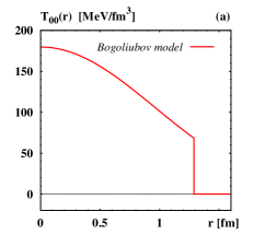
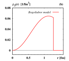
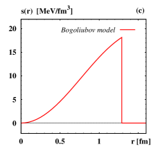
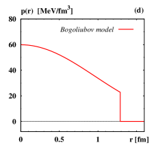
Figure 9: EMT densities as functions of $r$ in the Bogoliubov model: (a) energy density $T_{00}(r)$, (b) angular momentum density $\rho_{J}(r)$, (c) shear forces $s(r)$, and (d) pressure $p(r)$. This version of the Bogoliubov model corresponds to the bag model with the bag constant $B$ absent. The EMT densities are similar to the bag model except for the pressure which exhibits no node and does not comply with the von Laue condition, which means this is an inconsistent, unphysical solution.

IX Conclusions

In this work we have explored the bag model to study the EMT form factors $A^{a}(t)$, $J^{a}(t)$, $D^{a}(t)$, $\bar{c}^{a}(t)$ and the EMT densities. The quark contributions ($a=u,\,d$) to the EMT form factors are defined in terms of the single-quark wave-functions and the SU(4) spin-flavor factors needed to construct the nucleon wave-functions. The form factors factors $A^{a}(t)$, $J^{a}(t)$, $D^{a}(t)$ receive only quark contributions, i.e. in these cases the total form factors are given by $A(t)=A^{u}(t)+A^{d}(t)$ and analogous for $J(t)$, $D(t)$. In principle, also the bag makes contributions to form factors which can be interpreted as “gluonic” contributions. Only the form factor $\bar{c}^{a}(t)$ receives such a gluonic contribution.

It is crucial to check that all relations derived from $\partial_{\mu}T^{\mu\nu}=0$ are valid, and to demonstrate the mechanical stability of the model. The theoretical consistency is reflected in various ways. We have shown that the bag model description of the EMT form factors is consistent in the large-$N_{c}$ limit. The constraints $A(0)=1$ and $J(0)=\frac{1}{2}$ are satisfied, and $\sum_{a}\bar{c}^{a}(t)=0$ holds for all $t$. Since the bag contribution is not described in terms of a wave function, it was necessary to determine the gluonic form factor $\bar{c}^{G}(t)$ using a different method by resorting to the EMT density formalism. The large-$N_{c}$ formulation of the bag model correctly reproduces the general large-$N_{c}$ counting rules for the EMT form factors Goeke:2001tz . The usage of the large-$N_{c}$ limit has moreover the advantage of resolving technical problems associated with form factor calculations in “independent particle models” like the bag model. When considering the large-$N_{c}$ limit our expressions for the EMT form factors agree with those from Ref. Ji:1997gm . We have shown that the $1/N_{c}$ corrections associated with our large-$N_{c}$ treatment of the EMT form factors are relatively small for $|t|\ll M_{N}$.

The large-$N_{c}$ limit automatically provides a rigorous justification for the concept of 3D densities. We studied the energy density $T^{00}(r)$, the angular momentum density $J^{i}(\vec{r})=\epsilon^{ijk}r^{j}T^{0k}(\vec{r})$, and the distributions of shear forces and pressure related to the stress tensor $T^{ij}(\vec{r})$. We have shown that the bag model EMT densities comply with all general requirements including the von Laue condition which is a necessary condition for stability. The bag model also complies with analogous lower-dimensional stability conditions. Another important result is that the angular momentum density $J^{i}(\vec{r})$ in the bag model can be decomposed in monopole and quadrupole terms which are model-independently related to each other.

We presented an extensive study of the $D$-term in the bag model, not only for the nucleon but also for other hadrons including $N^{\star}$-resonances, vector mesons, $\Delta$-resonances, and hypothetical highly excited bag model states. We have shown that in all cases the $D$-term is negative. We made the interesting observation that asymptotically the $D$-terms grow as $D=-\,{\rm const}\times M^{8/3}$ with the mass $M$ of the excitation. Interestingly, the same asymptotic dependence was found for high excitations in the $Q$-ball system Mai:2012cx even though the internal structure of the excited states in the two systems is much different: for instance, the pressure in the $N^{\rm th}$ excited state exhibits $(2N+1)$-nodes in the $Q$-ball system, but one and only one node in the bag model. We are not aware whether the growth $D=-\,{\rm const}\times M^{8/3}$ of the $D$-term with the mass $M$ of the excitation is a general result, or a common peculiarity of these two (very different) systems. It will be interesting to investigate this result in other theoretical systems. At this point it is not known how to access information on the EMT form factors of $N^{\ast}$ states, but information on transition form factors can in principle be deduced from studies of hard exclusive reactions. This field has a lot of potential.

The study of excited states has brought very interesting insights. For instance, while the mass increases by about $50\,\%$ as one goes from the ground state (nucleon) to the first excited state (Roper), the internal pressure in the center and the $D$-term increase by factor 7. This finding supports the observations made in other systems that the $D$-term is a quantity which most strongly reflects the internal dynamics of the system and exhibits the strongest variations as one for instance considers higher excited states. The ground state and all excited states correspond to mininima of the action, and comply therefore with the necessary stability condition provided by the von Laue relation, and the $D$-terms are always negative. However, only the ground state is the global minimum of the action, and hence absolutely stable. The excited states correspond to local minima and can decay into the ground state.

We studied the $D$-term in three different limits: heavy quark limit, large bag-radius limit, and non-relativistic limit. The $D$-term assumes the same well-defined finite value in these three limits which can be computed analytically. This shows that the $D$-term is a property of all systems including non-relativistic systems. Since $D=0$ for a free fermion Hudson:2017oul , this also provides an illustration how e.g. even very small interactions in the bag model (in the limit of a very large bag radius) generate a non-zero $D$-term.

The bag model is at variance with chiral symmetry, and its oversimplified description cannot be expected to give accurate predictions. But one main goal of this work was to shed light on the interpretation of EMT form factors in terms of 3D densities. For this it is crucial to use a consistent theoretical framework, and the bag model provides this. The simplicity of this model is a crucial advantage when elucidating the concepts. For instance, it was observed in several models that the von Laue condition $\int_{0}^{\infty}dr\,r^{2}p(r)=0$ is related to the virial theorem. This is also the case in the bag model, and we were able to show that not only this but also the lower-dimensional analogs of the von Laue condition are satisfied provided one works with a solution satisfying the virial theorem. Another interesting observation is related to the mechanical stability requirement that the normal force per unit area $\frac{2}{3}s(r)+p(r)\geq 0$. This quantity is positive inside the bag, and the point where it drops to zero marks the “edge of the system,” i.e. the bag boundary in our case. Such an observation can only be obtained in a finite size system.

Finally, we studied the EMT densities in the Bogoliubov model Bogo:1967 , a predecessor of the bag model in which the bag contribution is absent and the bag radius needs to be fixed by hand. This model provides a counter-example for a framework where the nucleon is not consistently described. Fixing the bag radius by hand (rather than by means of a dynamical equation) corresponds to “external forces” which are not included in the Lagrangian. This implies an unphysical situation in which the EMT is not conserved and where the pressure has no node and the von Laue condition is not satisfied. From such a positive pressure one would obtain an unphysical positive $D$-term. This problem is solved in the bag model by introducing a non-zero bag constant $B$ in the Lagrangian.

It will be interesting to study the EMT form factors and the associated densities in other models whose nature is classical, quantum mechanical, or field theoretical. Such studies deepen our understanding of the hadron structure.

Acknowledgments. The authors are indebted to Cedric Lorcé, Maxim Polyakov and Leonard Schweitzer for valuable discussions. This work was supported by NSF grant no. 1812423 and DOE grant no. DE-FG02-04ER41309.

Appendix A Technical details and proofs

This Appendix contains technical details. Let us quote first the expressions for the first 3 spherical Bessel functions

$$j_{0}(x)=\frac{\sin x}{x}\,,\quad j_{1}(x)=\frac{\sin x}{x^{2}}-\frac{\cos x}{x},\quad j_{2}(x)=3\,\frac{\sin x}{x^{3}}-3\,\frac{\cos x}{x^{2}}-\frac{\sin x}{x}\,.$$ (57)

Below we shall also made use of the expansion of a plane wave $e^{i\vec{\Delta}\,\vec{r}}$ in terms of spherical Bessel functions and Legendre polynomials $P_{l}(x)$ as well as the orthogonality relation of the latter

$$e^{i\vec{q}\,\vec{r}}=\sum_{l=0}^{\infty}i^{l}(2l+1)\,j_{l}(qr)\,P_{l}(\cos\theta)\;,\quad\int_{-1}^{1}\!{\rm d}\cos\theta\;P_{l}(\cos\theta)P_{k}(\cos\theta)=\frac{2}{2l+1}\,\delta_{lk}\,.$$ (58)

In order to abbreviate the expressions below let us define the integrals over the combinations of spherical Bessel functions entering respectively the expressions for $p(r)$ and $s(r)$, namely

$$I_{n}^{p}(\omega)=\int_{0}^{\omega}\!{\rm d}x\;x^{n}\biggl{(}j_{0}(x)j_{1}^{\prime}(x)-j_{0}^{\prime}(x)j_{1}(x)+\frac{2}{x}j_{0}(x)j_{1}(x)\biggr{)}\,,$$

$$I_{n}^{s}(\omega)=\int_{0}^{\omega}\!{\rm d}x\;x^{n}\biggl{(}j_{0}(x)j_{1}^{\prime}(x)-j_{0}^{\prime}(x)j_{1}(x)-\frac{1}{x}j_{0}(x)j_{1}(x)\biggr{)}\,.$$ (59)

A.1 Virial theorem in general case

Let us generalize the virial theorem (26) to general (including excited) states with $m\neq 0$. In the general case the mass of a hadron is obtained by occupying $N_{\rm const}$ energy levels $\varepsilon_{i}=\Omega_{i}/R$ and adding the energy due to the bag,

$$M(R)=\frac{1}{R}\sum_{i}\Omega_{i}+\frac{4\pi}{3}\,BR^{3}$$ (60)

where the sum goes over the occupied levels $i=1,\;\dots\,,\;N_{\rm const}$ and $N_{\rm const}$ denotes the number of constituents with $N_{\rm const}=2$ for mesons and $N_{\rm const}=N_{c}$ for baryons.

The $\Omega_{i}=\sqrt{\omega_{i}^{2}+m^{2}R^{2}}$ depend on $R$ explicitly, and the $\omega_{i}$ implicitly through the transcendental equation (12). The derivative of $\omega_{i}$ with respect to $R$ is determined by differentiating Eq. (12) with respect to $R$ which, upon exploring (12) to eliminate trigonometric functions, yields

$$\frac{\partial\omega_{i}}{\partial R}=\frac{m\,\omega_{i}}{2\Omega_{i}(\Omega_{i}-1)+mR}\,.$$ (61)

Using the result (61) we obtain the virial theorem valid for $m\neq 0$ and excited states which is given by

$$M_{N}^{\prime}(R)=-\,\frac{1}{R^{2}}\;\sum_{i}\frac{2(\Omega_{i}-1)\omega_{i}^{2}}{2\Omega_{i}(\Omega_{i}-1)+mR}+4\pi\,R^{2}B\stackrel{{\scriptstyle!}}{{=}}0\quad\Leftrightarrow\quad 4\pi R^{4}B=\sum_{i}\frac{2(\Omega_{i}-1)\omega_{i}^{2}}{2\Omega_{i}(\Omega_{i}-1)+mR}$$ (62)

If one takes $m\to 0$ the derivative (61) vanishes and the virial theorem (62) reduces to Eq. (26) for the nucleon.

A.2 Proof of von Laue condition

For notational convenience we present the proof for the nucleon case. The generalization to other bag states is straight forward. Integrating $p(r)$ in Eq. (29) over $\!{\rm d}^{3}r$ and using the substitution $r\to x=\omega r/R$ yields

$$\int\!{\rm d}^{3}r\,p(r) = N_{c}\,A^{2}\;\alpha_{+}\alpha_{-}\,\frac{R^{2}}{3\omega_{0}^{2}}\;I_{2}^{p}(\omega_{0})-\frac{4\pi}{3}\,BR^{3}\,.$$ (63)

The integral over the Bessel functions $I_{2}^{p}(\omega_{0})$ is defined in Eq. (59) and yields

$$I_{2}^{p}(\omega_{0})=\frac{\omega_{0}^{2}-\sin^{2}\omega_{0}}{\omega_{0}}\,.$$ (64)

Inserting (64) into Eq. (63) we find

$$\int\!{\rm d}^{3}r\,p(r)=N_{c}\,A^{2}\;\alpha_{+}\alpha_{-}\,\frac{R^{2}}{3\omega_{0}^{2}}\;\frac{\omega_{0}^{2}-\sin^{2}\omega_{0}}{\omega_{0}}-\frac{4\pi}{3}\,BR^{3}\stackrel{{\scriptstyle!}}{{=}}0\,,$$ (65)

That Eq. (65) is zero becomes apparent after inserting the expressions for $A$ and $\alpha_{\pm}$ defined in the context of Eq. (11), exploring the transcendental equation (12) to eliminate trigonometric functions and some tedious algebra, which yields

$$\int\!{\rm d}^{3}r\,p(r)=\frac{N_{c}}{3R}\frac{2\omega_{0}^{2}(\Omega_{0}-1)}{2\Omega_{0}(\Omega_{0}-1)+mR}-\frac{4\pi}{3}\,BR^{3}=-\;\frac{1}{3}\;R\,M_{N}^{\prime}(R)\stackrel{{\scriptstyle!}}{{=}}0\,$$ (66)

where in the second step we made use of the virial theorem (62) for the nucleon case.

To prove the 2D analog of the von Laue condition we consider

$$\int_{0}^{\infty}\!{\rm d}r\;r\biggl{(}-\frac{1}{3}\,s(r)+p(r)\biggr{)}=N_{c}\,\frac{A^{2}}{4\pi}\;\alpha_{+}\alpha_{-}\,\frac{R}{3\omega}\biggl{[}-I_{1}^{s}(\omega_{0})+I_{1}^{p}(\omega_{0})\;\biggr{]}-\frac{1}{2}\,BR^{2}=-\;\frac{1}{8\pi}\;M_{N}^{\prime}(R)\stackrel{{\scriptstyle!}}{{=}}0\,,$$ (67)

where in the last step we used Eqs. (62, 65). Similarly for the 1D-version of the von Laue condition we find

$$\int_{0}^{\infty}\!{\rm d}r\,\biggl{(}-\frac{4}{3}\,s(r)+p(r)\biggr{)}=N_{c}\,\frac{A^{2}}{4\pi}\;\alpha_{+}\alpha_{-}\,\frac{1}{3}\biggl{[}-4I_{0}^{s}(\omega_{0})+I_{0}^{p}(\omega_{0})\biggr{]}-BR=-\;\frac{1}{4\pi R}\;M_{N}^{\prime}(R)\stackrel{{\scriptstyle!}}{{=}}0\,.$$ (68)

Notice that the integrals $I_{0}^{s}(\omega_{0})$, $I_{0}^{p}(\omega_{0})$, $I_{1}^{s}(\omega_{0})$, $I_{1}^{p}(\omega_{0})$ are well-defined but contain sine- and cosine-integral terms which cancel out in the linear combinations in the square brackets in (67, 68). The results (66, 67, 68) show that the von Laue condition and its lower-dimensional analogs are all satisfied if the virial theorem is satisfied.

A.3 Equivalence of $D$-term expressions

In this Section let us distinguish the expressions $D_{p}$ and $D_{s}$ for the $D$-term in terms of pressure and shear forces as defined in Eq. (7). For $D_{p}$ we have

$$D_{p}=M_{N}\int\!{\rm d}^{3}r\,r^{2}p(r)=M_{N}\biggl{(}N_{c}\,A^{2}\;\alpha_{+}\alpha_{-}\,\frac{R^{4}}{3\omega_{0}^{4}}I_{4}^{p}(\omega_{0})-\frac{4\pi}{5}\,BR^{5}\biggr{)}\,,$$ (69)

where the integral over Bessel functions yields

$$I_{4}^{p}(\omega_{0})=\frac{\omega_{0}^{3}}{3}+\omega_{0}-\omega_{0}\,\sin^{2}\omega_{0}-\sin\omega_{0}\,\cos\omega_{0}$$ (70)

Exploring the expression (65) for the von Laue condition to eliminate $B$ yields

$$D_{p}=M_{N}N_{c}\,A^{2}\;\alpha_{+}\alpha_{-}\,\frac{R^{4}}{3\omega_{0}^{4}}\biggl{(}-\frac{4}{15}\,\omega_{0}^{3}+\omega_{0}-\frac{2}{5}\omega_{0}\,\sin^{2}\omega_{0}-\sin\omega_{0}\,\cos\omega_{0}\biggr{)}$$ (71)

and corresponds to the expression quoted in Eq. (37).

To show that the expression in terms of shear forces yields the same result we consider

$$D_{s}=-\frac{4}{15}\,M_{N}\int\!{\rm d}^{3}r\,r^{2}s(r)=-\frac{4}{5}\,M_{N}N_{c}\,A^{2}\;\alpha_{+}\alpha_{-}\,\frac{R^{4}}{3\omega_{0}^{4}}I_{4}^{s}(\omega_{0})$$ (72)

with the integral over Bessel functions given by

$$I_{4}^{s}(\omega_{0})=\frac{\omega_{0}^{3}}{3}-\frac{5}{4}\,\omega_{0}+\frac{5}{4}\,\sin\omega_{0}\,\cos\omega_{0}+\frac{1}{2}\omega_{0}\,\sin^{2}\omega_{0}\,.$$ (73)

The difference of the two expressions for the $D$-term is

$$D_{p}-D_{s} =M_{N}N_{c}\,A^{2}\;\alpha_{+}\alpha_{-}\,\frac{R^{4}}{3\omega_{0}^{4}}\biggl{(}I_{4}^{p}(\omega_{0})+\frac{4}{5}\,I_{4}^{s}(\omega_{0})\biggr{)}-\frac{4}{5}\,\pi\,M_{N}BR^{5}=-\;\frac{1}{5}\;R^{3}M_{N}M_{N}^{\prime}(R)\stackrel{{\scriptstyle!}}{{=}}0$$ (74)

where in the last step we once more made use of Eqs. (62, 65). This proves that the expressions for the $D$-term in terms of $p(r)$ and $s(r)$ are equivalent.

A.4 Proof that $\bar{c}^{Q}(t)+\bar{c}^{G}(t)=0$

In the main text it was shown that at $t=0$ it is $\bar{c}^{Q}(0)+\bar{c}^{G}(0)=0$. We now wish to generalize this proof to $t\neq 0$. The proof is elementary but tedious such that it is worth showing it in some more detail. The starting point is $\bar{c}^{Q}(t)$ in (23c). We recall that $\vec{k}^{\,\prime}=\vec{k}+\vec{\Delta}$ with $\vec{\Delta}=(0,0,\Delta^{3})$ in our kinematics. The right-hand-side of (23c) is an even function of $\Delta^{3}$. To show this we replace $\Delta^{3}\to(-\Delta^{3})$ and subsequently substitute $k^{3}\to(-k^{3})$ which restores the starting expression. This proves that $\bar{c}^{Q}(t)$ can be understood as a function of $t=-\vec{\Delta}{}^{2}$ as it must for a form factor. In the next step we explore this to simplify the expression for $\bar{c}^{Q}(t)$ as follows. In the first term in the square brackets of (23c) we substitute $k^{3}\to k^{3}-\Delta^{3}$ and subsequently we explore that the function is even under $\Delta^{3}\to(-\Delta^{3})$, which restores the original expression but with $\vec{k}$ and $\vec{k}^{\,\prime}$ exchanged. This allows us to write Eq. (23c) as

$${\bar{c}}^{Q}(t)=-\;b\int\!\frac{\!{\rm d}^{3}k}{(2\pi)^{3}\!}\,(k^{\prime 3}+k^{3})\biggl{[}t_{0}(k^{\prime})t_{1}(k)\,e_{k}^{3}\biggr{]},\quad b=\frac{4\pi A^{2}R^{6}N_{c}}{M_{N}}\alpha_{+}\alpha_{-}$$ (75)

where $\vec{e}_{k}=\vec{k}/k$. It is convenient to work in coordinate space. In the formulas below Bessel functions $j_{l}$ with no argument will denote $j_{l}(w_{i}r/R)$ for notational simplicity, and the primes will denote derivatives with respect to $r$. In order to avoid total derivatives (which in general do not vanish in the finite volume integrals in the bag model and cause a proliferation of terms) we proceed by introducing a $\delta$-function as follows

$${\bar{c}}^{Q}(t)=-\;b\Biggl{[}\int\!\frac{\!{\rm d}^{3}k}{(2\pi)^{3}\!}\;t_{0}(k)k^{3}\int\!\frac{\!{\rm d}^{3}q}{(2\pi)^{3}\!}\,t_{1}(q)\,e_{q}^{3}+\int\!\frac{\!{\rm d}^{3}k}{(2\pi)^{3}\!}\,t_{0}(k)\int\!\frac{\!{\rm d}^{3}q}{(2\pi)^{3}\!}\,t_{1}(q)\,q^{3}e_{q}^{3}\Biggr{]}\int\!{\rm d}^{3}r\;e^{i\vec{r}(\vec{k}^{\,\prime}-\vec{q})}\,.$$ (76)

In the next step we invert the Fourier transforms, where $\Theta_{V}=\Theta(R-r)$ is used for brevity and we use identities

$$\int\!\frac{\!{\rm d}^{3}q}{(2\pi)^{3}\!}\,t_{0}(q)e^{i\vec{r}\vec{q}}=j_{0}\;\frac{\Theta_{V}}{4\pi R^{3}}\,,\quad\int\!\frac{\!{\rm d}^{3}q}{(2\pi)^{3}\!}\;\vec{e}_{q}t_{1}(q)\,e^{-i\vec{r}\vec{q}}=-i\vec{e}_{r}j_{1}\;\frac{\Theta_{V}}{4\pi R^{3}}\,,$$ (77)

where (as before) $j_{i}=j_{i}(\omega r/R)$ for brevity. This yields

$${\bar{c}}^{Q}(t) =\frac{b}{(4\pi R^{3})^{2}}\;\int\!\!{\rm d}^{3}r\,e^{i\vec{r}\vec{\Delta}}\Biggl{[}(e_{r}^{3})^{2}\biggl{(}j_{0}^{\prime}j_{1}-j_{0}j_{1}^{\prime}+\frac{j_{0}j_{1}}{r}\biggr{)}-\frac{j_{0}j_{1}}{r}\Biggr{]}\,\Theta_{V}\,.$$ (78)

Finally we explore that $e_{r}^{3}=\vec{e}_{z}\cdot\vec{e}_{r}=\cos\theta$ such that $(e_{r}^{3})^{2}=\frac{2}{3}P_{2}(\cos\theta)+\frac{1}{3}P_{0}(\cos\theta)$. Making use of the expansion of $e^{i\vec{r}\vec{\Delta}}$ and the orthogonality of Legendre polynomials in (58), we obtain

$${\bar{c}}^{Q}(t)=\frac{b}{(4\pi R^{3})^{2}}\;\int_{V}\!\!{\rm d}^{3}r\,\Biggl{[}\biggl{(}\underbrace{-\frac{2}{3}j_{2}(\Delta r)+\frac{1}{3}j_{0}(\Delta r)}_{\frac{1}{\Delta}\,j_{1}^{\prime}(\Delta r)}\biggr{)}\biggl{(}j_{0}^{\prime}j_{1}-j_{0}j_{1}^{\prime}\biggr{)}+\biggl{(}\underbrace{-\frac{1}{3}j_{2}(\Delta r)-\frac{1}{3}j_{0}(\Delta r)}_{=-\frac{j_{1}(\Delta r)}{\Delta r}}\biggr{)}\frac{2j_{0}j_{1}}{r}\Biggr{]}$$ (79)

where the underbraces indicate useful identities. Another helpful identity is $2j_{0}j_{1}=-\frac{\partial\;}{\partial r}[r^{2}(j_{0}^{\prime}j_{1}-j_{0}j_{1}^{\prime})]$. After integrating over the solid angle we find that the $r$-integrand is a total derivative

$${\bar{c}}^{Q}(t) =\frac{4\pi b}{(4\pi R^{3})^{2}\Delta}\;\int_{0}^{R}\!{\rm d}r\Biggl{[}\frac{\partial\;}{\partial r}\biggl{[}j_{1}(\Delta r)\;r^{2}\biggl{(}j_{0}^{\prime}j_{1}-j_{0}j_{1}^{\prime}\biggr{)}\biggr{]}\Biggr{]}=-\,c_{0}\,\frac{j_{1}(\Delta R)}{\Delta R}\,.$$ (80)

In the massless case the prefactor $c_{0}$ is given by

$$c_{0}=\frac{b}{4\pi R^{3}}\frac{\omega_{0}}{R}\;\biggl{(}j_{0}(\omega_{0})j_{1}^{\prime}(\omega_{0})-j_{0}^{\prime}(\omega_{0})j_{1}(\omega_{0})\biggr{)}=\frac{3}{4}$$ (81)

which follows from using the transcendental equation (12). In the massive case the result is a different fraction, and the last step is lengthier and one has to use the expression for $B$ from the massive virial theorem to show that the constraint $\sum_{i}\bar{c}^{i}(t)$ holds also here.

A.5 EMT form factor of the anti-symmetric EMT

For completeness we discuss the form factors of the canonical EMT defined by $T^{\mu\nu,q}_{\rm can}=\frac{1}{2}\overline{\psi}_{q}(-i\gamma^{\mu}\overset{\leftarrow}{\partial}{}^{\nu}+i\gamma^{\mu}\overset{\rightarrow}{\partial}{}^{\nu})\psi_{q}$. The canonical EMT can be decomposed in two parts: a symmetric part whose form factors $A^{q}(t)$, $J^{q}(t)$, $D^{q}(t)$, $\bar{c}^{q}(t)$ were discussed in the main text, and an antisymmetric part which is characterized by a single form factor Bakker:2004ib

$$\langle p^{\prime}|\frac{1}{2}\biggl{(}\hat{T}^{\mu\nu,q}_{\rm can}(0)-\hat{T}^{\nu\mu,q}_{\rm can}(0)\biggr{)}|p\rangle=F_{\rm can}^{q}(t)\ \bar{u}(p^{\prime})\,\frac{i(P^{\mu}\sigma^{\nu\rho}-P^{\nu}\sigma^{\mu\rho})\Delta_{\rho}}{4M_{N}}u(p)\,,$$ (82)

which in the bag model is given by

$$F_{\rm can}^{q}(t)=4\pi A^{2}R^{6}\int\!\frac{\!{\rm d}^{3}k}{(2\pi)^{3}\!}\,\biggl{[}2\alpha_{+}\alpha_{-}\frac{\varepsilon_{0}}{\Delta^{3}}\biggl{(}t_{0}(k^{\prime})t_{1}(k)\,\frac{k^{3}}{k}-t_{0}(k)t_{1}(k^{\prime})\,\frac{k^{\prime 3}}{k^{\prime}}\biggr{)}+k_{\perp}^{2}\alpha_{-}^{2}\frac{t_{1}(k)}{k}\,\frac{t_{1}(k^{\prime})}{k^{\prime}}\biggr{]}\,.$$ (83)

The expression (83) agrees up to the sign with the bag model results for the axial form factor $G_{A}^{q}(t)$. Thus, we recover $F_{\rm can}^{q}(t)=-G_{A}^{q}(t)$ which is a model independent result Bakker:2004ib . This shows that also the canonical EMT is consistently described within the bag model.

References

-
(1)
I. Y. Kobzarev and L. B. Okun,
Zh. Eksp. Teor. Fiz. 43, 1904 (1962)
[Sov. Phys. JETP 16, 1343 (1963)].
H. Pagels, Phys. Rev. 144, 1250 (1966). - (2) D. Müller, D. Robaschik, B. Geyer, F.-M. Dittes and J. Hořejši, Fortsch. Phys. 42, 101 (1994) [hep-ph/9812448].
- (3) X. D. Ji, Phys. Rev. Lett. 78, 610 (1997) [hep-ph/9603249]. X. D. Ji, Phys. Rev. D 55, 7114 (1997) [hep-ph/9609381].
- (4) A. V. Radyushkin, Phys. Lett. B 380, 417 (1996) [hep-ph/9604317]; Phys. Lett. B 385, 333 (1996) [hep-ph/9605431]; A. V. Radyushkin, Phys. Rev. D 56, 5524 (1997) [hep-ph/9704207].
- (5) J. C. Collins, L. Frankfurt and M. Strikman, Phys. Rev. D 56, 2982 (1997) [hep-ph/9611433].
- (6) K. Goeke, M. V. Polyakov and M. Vanderhaeghen, Prog. Part. Nucl. Phys. 47, 401 (2001).
-
(7)
M. Diehl,
Phys. Rept. 388 (2003) 41.
A. V. Belitsky and A. V. Radyushkin, Phys. Rept. 418, 1 (2005).
S. Boffi and B. Pasquini, Riv. Nuovo Cim. 30, 387 (2007) [arXiv:0711.2625 [hep-ph]]. - (8) M. V. Polyakov, Phys. Lett. B 555, 57 (2003) [hep-ph/0210165].
- (9) M. V. Polyakov and P. Schweitzer, Int. J. Mod. Phys. A 33, 1830025 (2018).
- (10) X. D. Ji, W. Melnitchouk and X. Song, Phys. Rev. D 56, 5511 (1997) [hep-ph/9702379].
- (11) V. Y. Petrov, P. V. Pobylitsa, M. V. Polyakov, I. Börnig, K. Goeke and C. Weiss, Phys. Rev. D 57, 4325 (1998).
- (12) P. Schweitzer, S. Boffi and M. Radici, Phys. Rev. D 66, 114004 (2002) [hep-ph/0207230].
- (13) J. Ossmann, M. V. Polyakov, P. Schweitzer, D. Urbano and K. Goeke, Phys. Rev. D 71, 034011 (2005) [hep-ph/0411172].
- (14) M. Wakamatsu and H. Tsujimoto, Phys. Rev. D 71, 074001 (2005) [arXiv:hep-ph/0502030].
- (15) M. Wakamatsu and Y. Nakakoji, Phys. Rev. D 74, 054006 (2006) [arXiv:hep-ph/0605279].
- (16) K. Goeke, J. Grabis, J. Ossmann, M. V. Polyakov, P. Schweitzer, A. Silva, D. Urbano, Phys. Rev. D 75, 094021 (2007).
- (17) K. Goeke, J. Grabis, J. Ossmann, P. Schweitzer, A. Silva and D. Urbano, Phys. Rev. C 75, 055207 (2007).
- (18) M. Wakamatsu, Phys. Lett. B 648, 181 (2007) [hep-ph/0701057].
- (19) C. Cebulla, K. Goeke, J. Ossmann and P. Schweitzer, Nucl. Phys. A 794, 87 (2007) [hep-ph/0703025].
- (20) H. C. Kim, P. Schweitzer and U. Yakhshiev, Phys. Lett. B 718, 625 (2012) [arXiv:1205.5228 [hep-ph]].
- (21) J. H. Jung, U. Yakhshiev and H. C. Kim, J. Phys. G 41, 055107 (2014) [arXiv:1310.8064 [hep-ph]].
- (22) J. H. Jung, U. Yakhshiev, H. C. Kim and P. Schweitzer, Phys. Rev. D 89, 114021 (2014) [arXiv:1402.0161 [hep-ph]].
- (23) I. A. Perevalova, M. V. Polyakov and P. Schweitzer, Phys. Rev. D 94, 054024 (2016) [arXiv:1607.07008 [hep-ph]].
- (24) Z. Abidin and C. E. Carlson, Phys. Rev. D 77, 095007 (2008) [arXiv:0801.3839 [hep-ph]].
- (25) Z. Abidin and C. E. Carlson, Phys. Rev. D 77, 115021 (2008) [arXiv:0804.0214 [hep-ph]].
- (26) S. J. Brodsky and G. F. de Teramond, Phys. Rev. D 78, 025032 (2008) [arXiv:0804.0452 [hep-ph]].
- (27) Z. Abidin and C. E. Carlson, Phys. Rev. D 79, 115003 (2009).
- (28) K. A. Mamo and I. Zahed, arXiv:1910.04707 [hep-ph].
- (29) E. Megias, E. Ruiz Arriola, L. L. Salcedo and W. Broniowski, Phys. Rev. D 70, 034031 (2004).
- (30) E. Megias, E. Ruiz Arriola and L. L. Salcedo, Phys. Rev. D 72, 014001 (2005).
- (31) W. Broniowski and E. R. Arriola, Phys. Rev. D 78, 094011 (2008).
- (32) N. Kumar, C. Mondal and N. Sharma, Eur. Phys. J. A 53, 237 (2017) [arXiv:1712.02110 [hep-ph]].
- (33) D. Chakrabarti, C. Mondal and A. Mukherjee, Phys. Rev. D 91, 114026 (2015).
- (34) M. Mai and P. Schweitzer, Phys. Rev. D 86, 076001 (2012) [arXiv:1206.2632 [hep-ph]].
- (35) M. Mai and P. Schweitzer, Phys. Rev. D 86, 096002 (2012) [arXiv:1206.2930 [hep-ph]].
- (36) M. Cantara, M. Mai and P. Schweitzer, Nucl. Phys. A 953, 1 (2016) [arXiv:1510.08015 [hep-ph]].
- (37) I. E. Gulamov, E. Y. Nugaev, A. G. Panin and M. N. Smolyakov, Phys. Rev. D 92, 045011 (2015) [arXiv:1506.05786 [hep-th]].
- (38) E. Nugaev and A. Shkerin, arXiv:1905.05146 [hep-th].
- (39) J. Hudson and P. Schweitzer, Phys. Rev. D 96, 114013 (2017) [arXiv:1712.05316 [hep-ph]].
- (40) A. Freese and I. C. Cloët, Phys. Rev. C 100, 015201 (2019).
- (41) A. Freese and I. C. Cloët, arXiv:1907.08256 [nucl-th].
- (42) A. V. Belitsky and X. Ji, Phys. Lett. B 538, 289 (2002) [hep-ph/0203276].
- (43) S. I. Ando, J. W. Chen and C. W. Kao, Phys. Rev. D 74, 094013 (2006) [hep-ph/0602200].
- (44) M. Diehl, A. Manashov and A. Schäfer, Eur. Phys. J. A 29, 315 (2006) [hep-ph/0608113].
- (45) P. Masjuan, E. Ruiz Arriola and W. Broniowski, Phys. Rev. D 87, 014005 (2013) [arXiv:1210.0760 [hep-ph]].
- (46) B. Pasquini, M. V. Polyakov and M. Vanderhaeghen, Phys. Lett. B 739, 133 (2014) [arXiv:1407.5960 [hep-ph]].
- (47) N. Mathur, S. J. Dong, K. F. Liu, L. Mankiewicz and N. C. Mukhopadhyay, Phys. Rev. D 62, 114504 (2000) [arXiv:hep-ph/9912289].
-
(48)
P. Hägler et al. [LHPC and SESAM Collaborations],
Phys. Rev. D 68, 034505 (2003).
M. Göckeler et al. [QCDSF Collaboration], Phys. Rev. Lett. 92, 042002 (2004) [hep-ph/0304249]. - (49) P. Hägler et al. [LHPC Collaboration], Phys. Rev. D 77, 094502 (2008).
- (50) P. E. Shanahan and W. Detmold, Phys. Rev. D 99, 014511 (2019); Phys. Rev. Lett. 122, 072003 (2019).
-
(51)
I. V. Anikin,
Phys. Rev. D 99, 094026 (2019).
K. Azizi and U. Özdem, arXiv:1908.06143 [hep-ph]. - (52) I. R. Gabdrakhmanov and O. V. Teryaev, Phys. Lett. B 716, 417 (2012) [arXiv:1204.6471 [hep-ph]].
- (53) S. Friot, B. Pire and L. Szymanowski, Phys. Lett. B 645, 153 (2007) [hep-ph/0611176].
- (54) M. V. Polyakov and C. Weiss, Phys. Rev. D 60, 114017 (1999) [hep-ph/9902451].
- (55) O. V. Teryaev, Phys. Lett. B 510, 125 (2001) [hep-ph/0102303].
- (56) S. Kumano, Q. T. Song, O. V. Teryaev, Phys. Rev. D 97, 014020 (2018) [arXiv:1711.08088 [hep-ph]].
- (57) V. D. Burkert, L. Elouadrhiri, and F. X. Girod, Nature 557, 396 (2018).
- (58) K. Kumerički, Nature 570, E1 (2019).
- (59) A. Chodos, R. L. Jaffe, K. Johnson, C. B. Thorn and V. F. Weisskopf, Phys. Rev. D 9, 3471 (1974).
- (60) A. Chodos, R. L. Jaffe, K. Johnson and C. B. Thorn, Phys. Rev. D 10, 2599 (1974).
- (61) T. A. DeGrand, R. L. Jaffe, K. Johnson and J. E. Kiskis, Phys. Rev. D 12, 2060 (1975).
- (62) R. L. Jaffe, Phys. Rev. D 11, 1953 (1975).
- (63) L. S. Celenza and C. M. Shakin, Phys. Rev. C 27, 1561 (1983) Erratum: [Phys. Rev. C 39, 2477 (1989)].
- (64) R. L. Jaffe and X. D. Ji, Nucl. Phys. B 375, 527 (1992).
- (65) A. Courtoy, F. Fratini, S. Scopetta and V. Vento, Phys. Rev. D 78, 034002 (2008) [arXiv:0801.4347 [hep-ph]].
- (66) H. Avakian, A. V. Efremov, P. Schweitzer and F. Yuan, Phys. Rev. D 78, 114024 (2008) [arXiv:0805.3355 [hep-ph]].
- (67) H. Avakian, A. V. Efremov, P. Schweitzer and F. Yuan, Phys. Rev. D 81, 074035 (2010) [arXiv:1001.5467 [hep-ph]].
- (68) H. M. Chang, A. V. Manohar and W. J. Waalewijn, Phys. Rev. D 87, 034009 (2013) [arXiv:1211.3132 [hep-ph]].
- (69) M. Rinaldi, S. Scopetta and V. Vento, Phys. Rev. D 87, 114021 (2013) [arXiv:1302.6462 [hep-ph]].
- (70) C. Lorcé, L. Mantovani and B. Pasquini, Phys. Lett. B 776, 38 (2018) [arXiv:1704.08557 [hep-ph]].
- (71) P. Schweitzer and K. Tezgin, Phys. Lett. B 796, 47 (2019) [arXiv:1905.12336 [hep-ph]].
- (72) M. V. Polyakov and P. Schweitzer, arXiv:1801.05858 [hep-ph].
- (73) M. V. Polyakov and H. D. Son, JHEP 1809, 156 (2018).
- (74) C. Lorcé, H. Moutarde and A. P. Trawiński, Eur. Phys. J. C 79, 89 (2019).
- (75) M. V. Polyakov and P. Schweitzer, arXiv:1812.06143 [hep-ph].
- (76) M. V. Polyakov and B. D. Sun, Phys. Rev. D 100, 036003 (2019) [arXiv:1903.02738 [hep-ph]].
- (77) W. Cosyn, S. Cotogno, A. Freese and C. Lorcé, Eur. Phys. J. C 79, 476 (2019)
- (78) A. W. Thomas and W. Weise, Berlin, Germany: Wiley-VCH (2001) 389 pages.
- (79) P. N. Bogoliubov, Ann. Inst. Henri Poncaré 8 (1967) 163.
- (80) J. Hudson and P. Schweitzer, Phys. Rev. D 97, 056003 (2018) [arXiv:1712.05317 [hep-ph]].
- (81) M. J. Neubelt, A. Sampino, J. Hudson, K. Tezgin and P. Schweitzer, PoS DIS 2019, 210 (2019) [arXiv:1907.11185 [hep-ph]].
- (82) R. G. Sachs, Phys. Rev. 126, 2256 (1962).
- (83) P. Lowdon, K. Y. J. Chiu and S. J. Brodsky, Phys. Lett. B 774, 1 (2017) [arXiv:1707.06313 [hep-th]].
- (84) S. Cotogno, C. Lorcé and P. Lowdon, Phys. Rev. D 100, 045003 (2019) [arXiv:1905.11969 [hep-th]].
- (85) G. Karl and J. E. Paton, Phys. Rev. D 30, 238 (1984).
- (86) R. E. Peierls and J. Yoccoz, Proc. Phys. Soc. A 70, 381 (1957).
- (87) X. M. Wang, X. T. Song and P. C. Yin, Hadronic J. 6, 985 (1983).
- (88) X. D. Ji, Phys. Lett. B 254 (1991) 456.
- (89) C. Lorcé, private communication (2017).
- (90) M. von Laue, Ann. Phys. (Leipzig) 340, 524 (1911).
- (91) M. V. Polyakov and P. Schweitzer, in Frascati Physics Series Vol. 69, Proceedings of “Photon 2019,” page 31 (2019).
- (92) P. Hasenfratz and J. Kuti, Phys. Rept. 40, 75 (1978).
- (93) V. A. Novikov and M. A. Shifman, Z. Phys. C 8, 43 (1981).
- (94) M. B. Voloshin and V. I. Zakharov, Phys. Rev. Lett. 45, 688 (1980).
- (95) M. B. Voloshin and A. D. Dolgov, Sov. J. Nucl. Phys. 35, 120 (1982) [Yad. Fiz. 35, 213 (1982)].
- (96) H. Leutwyler and M. A. Shifman, Phys. Lett. B 221, 384 (1989).
- (97) J. F. Donoghue and K. Johnson, Phys. Rev. D 21, 1975 (1980).
- (98) A. W. Thomas, Adv. Nucl. Phys. 13, 1 (1984).
- (99) V. D. Burkert and C. D. Roberts, Rev. Mod. Phys. 91, 011003 (2019).
-
(100)
B. L. G. Bakker, E. Leader and T. L. Trueman,
Phys. Rev. D 70, 114001 (2004)
[hep-ph/0406139].
E. Leader and C. Lorcé, Phys. Rept. 541, 163 (2014) [arXiv:1309.4235 [hep-ph]].